Cluster mean-field signature of entanglement entropy in bosonic superfluid-insulator transitions

Abstract

Entanglement entropy (EE), a fundamental conception in quantum information for characterizing entanglement, has been extensively employed to explore quantum phase transitions (QPTs). Although the conventional single-site mean-field (MF) approach successfully predicts the emergence of QPTs, it fails to include any entanglement. Here, for the first time, in the framework of a cluster MF treatment, we extract the signature of EE in the bosonic superfluid-insulator (SI) transitions. We consider a trimerized Kagomé lattice of interacting bosons, in which each trimer is treated as a cluster, and implement the cluster MF treatment by decoupling all inter-trimer hopping. In addition to superfluid and integer insulator phases, we find that fractional insulator phases appear when the tunneling is dominated by the intra-trimer part. To quantify the residual bipartite entanglement in a cluster, we calculate the second-order Rényi entropy, which can be experimentally measured by quantum interference of many-body twins. The second-order Rényi entropy itself is continuous everywhere, however, the continuousness of its first-order derivative breaks down at the phase boundary. This means that the bosonic SI transitions can still be efficiently captured by the residual entanglement in our cluster MF treatment. Besides to the bosonic SI transitions, our cluster MF treatment may also be used to capture the signature of EE for other QPTs in quantum superlattice models.

I introduction

Quantum entanglement Horodecki et al. (2009); Laorencie (2015); Carmeli et al. (2016) an essential resource enabling modern quantum technologies, has a broad impact in understanding quantum phase transitions (QPTs) Amico et al. (2008); Eisert et al. (2010). The entanglement entropy (EE), which quantifies bipartite entanglement (the entanglement between two subsystems), is a typical measure of entanglement Bennett et al. (1996). The signature of EE in QPTs has been studied in various many-body quantum systems, such as, spin system Osborne and Nielsen (2002); Vidal et al. (2003); Latorre and Vidal (2004); Carrasco et al. (2016), Fermi-Hubbard system Gu et al. (2004); Anfossi et al. (2005, 2006); You (2014) and Bose-Hubbard (BH) system Buonsante and Vezzani (2007); Lauchli and Kollath (2008); Silva-Valencia and Souza (2011); Pino et al. (2012); Alba et al. (2013); Frérot and Roscilde (2016). Recently, the second-order Rényi EE in a bosonic superfluid-insulator (SI) transition Jaksch et al. (1998); Greiner et al. (2002) has been measured in an experiment of ultracold bosonic atoms in optical lattices Islam et al. (2015). However, a biggest challenge is to efficiently and rapidly extract the signature of EE for QPTs in an interacting many-body quantum system.

Up to now, several different methods have been devoted to calculate the EE in various BH systems. For one-dimensional BH systems, the von Neumann entropy (i.e. the first-order Rényi EE) has been calculated by exact diagonalization Buonsante and Vezzani (2007), density matrix renormalization group (DMRG) Lauchli and Kollath (2008), time-evolving block decimation (TEBD) Pino et al. (2012) and slave-boson approach Frérot and Roscilde (2016). For two-dimensional BH systems, the Rényi EE up to second-order has been calculated by DMRG Alba et al. (2013). For completely connected graphs, the von Neumann entropy has been calculated by exact diagonalization Buonsante and Vezzani (2007); Giorda and Zanardi (2004). For a Kagomé lattice, the topological EE has been calculated by quantum Monte Carlo (QMC) simulation Isakov et al. (2011). Most of these works concentrate on the von Neumann entropy, the first-order Rényi EE, which is hard to be measured in experiments. Moreover, although the von Neumann entropies for infinite systems may successfully identify QPTs, their calculations request large computational resources and long computational times. As the second-order Rényi EE is experimentally measurable, it is vital to calculate such a measurable EE via an efficient method, which does not cost too much computational resources and times.

It is well-known that the mean-field (MF) approach may successfully predict the emergence of most QPTs in BH systems. However, the conventional single-site MF approach Fisher et al. (1989); Sheshadri et al. (1993); van Oosten et al. (2001), which is based upon the product state ansatz of single-site states, does not include any entanglement. Therefore, it is impossible to extract EE via the conventional single-site MF approach. Fortunately, the cluster MF approach, or more generally, the composite boson MF theory Huerga et al. (2013), can reserve partial entanglement and have explored several new phases not found by the conventional single-site MF approach Buonsante et al. (2004); Pisarski et al. (2011); McIntosh et al. (2012); Lühmann (2013); Deng et al. (2015). Can the cluster MF approach efficiently capture the signature of EE in the emerged QPTs?

In this article, we explore the cluster MF signature of EE for the bosonic SI transitions in a trimerized Kagomé lattice (TKL). In the framework of our cluster MF treatment, each trimer in the TKL is treated as a cluster and the inter-trimer hopping is decoupled by using the MF approximation. Therefore the ground-state (GS) of the whole system is a product of single-cluster states. By diagonalizing the MF Hamiltonian, we obtain its GS through a standard self-consistent procedure. By calculating the order parameter and the filling number, we find that the GS phase diagram include three different types of phases: superfluid, integer insulator (IntI) and fractional insulator (FracI). By analyzing the second-order Rényi EE, we find that the discontinuousness of its first-order derivative corresponds to the critical point of the bosonic SI transitions. Our results clearly show that the cluster MF treatment can still efficiently capture the signature of EE in the bosonic SI transitions. As the cluster MF treatment have successfully predicted the appearance of most QPTs in quantum superlattice models, we believe it may also efficiently capture the signature of EE in those QPTs.

The article structure is as follows. In this section, we introduce the related backgrounds and our motivation. In Sec. II, we give the Hamiltonian for our physical system. In Sec. III, we present our cluster MF treatment and obtain the ground-state phase diagram. In Sec. IV, we calculate the second-order Rényi EE and its first-order derivative and then show the relation between the first-order derivative and the phase transition. In Sec. V, we discuss the experimental possibility. In the last section, we conclude and discuss our results.

II model

We consider an ensemble of interacting ultracold Bose atoms confined in a two-dimensional optical superlattice,

$$V(\mathbf{r})=V_{0}\sum_{i=1}^{3} \Big{[} \cos\left(\mathbf{k}_{i}\cdot\mathbf{r}+\tfrac{3\sigma_{i}\phi}{2}\right)+2\cos\left(\tfrac{\mathbf{k}_{i}\cdot\mathbf{r}}{3}+\tfrac{\sigma_{i}\phi}{2}\right)$$ (1)

$$+4\cos\left(\tfrac{\mathbf{k}_{i}\cdot\mathbf{r}}{9}+\tfrac{\sigma_{i}\phi}{6}\right)\Big{]}^{2},$$

where $\mathbf{k}_{1}=k(\frac{1}{2},\frac{\sqrt{3}}{2})$, $\mathbf{k}_{2}=k(\frac{1}{2},-\frac{\sqrt{3}}{2})$, $\mathbf{k}_{3}=k(-1,0)$, and $\sigma_{1}=-\sigma_{2}=\sigma_{3}=1$. The potential depth $V_{0}$ is proportional to the laser intensity. The degree of trimerization can be tuned by varying the phase $\phi$ Santos et al. (2004); Damski et al. (2005); Lee2006 . The above potential forms a TKL lattice, see the inset of Fig. 1.

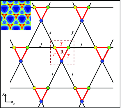
Figure 1: (color online). The schematic diagram for the trimerized Kagomé lattice. The unit cell is labelled by R. The lattice sites in the same color are equivalent. The red and the black bonds denote the intra-cell hopping $T$ and the inter-cell hopping $J$, respectively. The inset shows optical lattice potential, in which the darkest red region denotes the potential minimum.

The atom-atom interaction is described by the contact interaction

$$U_{c}(\mathbf{r}-\mathbf{r}^{\prime})=\frac{4\pi\hbar^{2}a_{s}}{m}\delta(\mathbf{r}-\mathbf{r}^{\prime})=g\delta(\mathbf{r}-\mathbf{r}^{\prime}),$$ (2)

where $m$ is the atomic mass and $a_{s}$ is the $s$-wave scattering length. In the second quantization theory, the system obeys the Hamiltonian

$$\hat{H} = \int\mathrm{d}\mathbf{r}\hat{\psi}^{\dagger}(\mathbf{r})\left[-\frac{\hbar^{2}\nabla^{2}}{2m}+V(\mathbf{r})-\mu\right]\hat{\psi}(\mathbf{r})$$ (3)

$$+ \frac{1}{2}\int\mathrm{d}\mathbf{r}\mathrm{d}\mathbf{r}^{\prime}\hat{\psi}^{\dagger}(\mathbf{r})\hat{\psi}^{\dagger}(\mathbf{r}^{\prime})U_{c}(\mathbf{r}-\mathbf{r}^{\prime})\hat{\psi}(\mathbf{r}^{\prime})\hat{\psi}(\mathbf{r}),$$

with the chemical potential $\mu$ and the bosonic field operator $\hat{\psi}(\mathbf{r})$. If the potential is sufficiently deep, the atoms will only occupy the lowest band and the field operator in terms of the lowest-band Wannier functions, the above Hamiltonian can be simplified as

$$\hat{H}_{\mathrm{BH}} = -T\sum_{\langle\mathrm{R}i,\mathrm{R}j\rangle}{\hat{a}^{\dagger}_{\mathrm{R}i}\hat{a}_{\mathrm{R}j}}-J\sum_{\begin{subarray}{c}\langle\mathrm{R}i,\mathrm{R^{\prime}}j\rangle,\mathrm{R}^{\prime}\neq\mathrm{R}\end{subarray}}{\hat{a}^{\dagger}_{\mathrm{R}i}\hat{a}_{\mathrm{R^{\prime}}j}}$$ (4)

$$+\frac{U}{2}\sum_{\mathrm{R}i}{\hat{n}_{\mathrm{R}i}(\hat{n}_{\mathrm{R}i}-1)}-\mu\sum_{\mathrm{R}i}{\hat{n}_{\mathrm{R}i}},$$

with $\hat{a}^{\dagger}_{\mathrm{R}i}$($\hat{a}_{\mathrm{R}i}$) creating (annihilating) a boson at the $i$-th site of the $\mathrm{R}$-th trimer. In Fig. 1, the lattice sites in blue, yellow and green are labelled as 1, 2 and 3, respectively. Here, $\hat{n}_{\mathrm{R}i}=\hat{a}^{\dagger}_{\mathrm{R}i}\hat{a}_{\mathrm{R}i}$ is the number operator, $T$ and $J$ are respectively the intra- and inter-trimer hopping strengthes, $U$ is the on-site interaction and $\mu$ is the chemical potential. The summations of $\mathrm{R}i$ and $\langle{\mathrm{R}i,\mathrm{R^{\prime}}j}\rangle$ comprise all lattice sites in the whole system and all nearest neighbor sites in different trimers, respectively. For convenience, we define $\beta=J/T$, the ratio between inter- and intra-trimer hopping strengths. Here we concentrate on the trimerized system of repulsive interaction, i.e., $\beta<1$ and $U>0$.

III cluster mean-field phase diagram

In this section, we show how to obtain the ground-state phase diagram with the cluster mean-field approach. In the first subsection, we present our cluster mean-field treatment for determining the ground states. In the last subsection, we give the ground-state phase diagram by calculating the order parameters.

III.1 Cluster mean-field treatment

The conventional single-site MF approach decouples the whole lattice into single sites which interact with the surrounding sites through mean fields. Based upon the equivalence of all single sites, the mean fields of the surrounding sites is thus replaced by the mean field of the site itself. Thus, the MF version of the original Hamiltonian can be viewed as a sum of single-site Hamiltonians.

The cluster MF approach we use is an extension of the single-site MF approach. It decouples the whole system as clusters of multiple lattice sites, in which the inter-cluster coupling are decoupled and the intra-clulster coupling are kept unchanged. In the TKL, we regard each trimer as a cluster and implement the standard MF decoupling for different trimers,

$$\hat{a}^{\dagger}_{\mathrm{R}i}\hat{a}_{\mathrm{R}^{\prime}j} \rightarrow \langle\hat{a}^{\dagger}_{\mathrm{R}i}\rangle\hat{a}_{\mathrm{R}^{\prime}j}+\hat{a}^{\dagger}_{\mathrm{R}i}\langle\hat{a}_{\mathrm{R}^{\prime}j}\rangle-\langle\hat{a}^{\dagger}_{\mathrm{R}i}\rangle\langle\hat{a}_{\mathrm{R}^{\prime}j}\rangle.$$ (5)

By introducing the order parameter $\Psi_{\mathrm{R}i}=\langle\hat{a}_{\mathrm{R}i}\rangle$ and substituting Eq. (5) into Eq. (4), we obtain the MF Hamiltonian

$$\hat{H}_{\mathrm{MF}}=\sum_{\mathrm{R}}\hat{H}_{\mathrm{MF}}^{\mathrm{R}},$$ (6)

with the single-cluster MF Hamiltonian

$$\hat{H}_{\mathrm{MF}}^{\mathrm{R}}\!= - T\sum_{\langle i,j\rangle}{\hat{a}^{\dagger}_{\mathrm{R}i}\hat{a}_{\mathrm{R}j}}$$ (7)

$$- J\sum_{\begin{subarray}{c}\langle\mathrm{R^{\prime}}j,\mathrm{R}i\rangle\\ \mathrm{R}^{\prime}\neq\mathrm{R}\end{subarray}}[\hat{a}^{\dagger}_{\mathrm{R}i}\Psi_{\mathrm{R^{\prime}}j}+\hat{a}_{\mathrm{R}i}\Psi^{*}_{\mathrm{R^{\prime}}j}-\mathrm{Re}(\Psi_{\mathrm{R}i}^{*}\Psi_{\mathrm{R^{\prime}}j})]$$

$$+ \frac{U}{2}\sum_{i}{\hat{n}_{\mathrm{R}i}(\hat{n}_{\mathrm{R}i}-1)}-\mu\sum_{i}{\hat{n}_{\mathrm{R}i}}.$$

The whole GS can be expressed as a product of the single-cluster states,

$$\left|{\Phi_{\mathrm{MF}}}\right\rangle=\otimes_{\mathrm{R}}\left|{\Phi_{\mathrm{MF}}^{\mathrm{R}}}\right\rangle.$$ (8)

Thus, the eigenequation $\hat{H}_{\mathrm{MF}}\left|{\Phi_{\mathrm{MF}}}\right\rangle=E\left|{\Phi_{\mathrm{MF}}}\right\rangle$ of the whole system can be reduced to the single-cluster eigenequation

$$\hat{H}_{\mathrm{MF}}^{\mathrm{R}}\left|{\Phi_{\mathrm{MF}}^{\mathrm{R}}}\right\rangle=E_{\mathrm{R}}\left|{\Phi_{\mathrm{MF}}^{\mathrm{R}}}\right\rangle$$ (9)

with $E=\sum_{\mathrm{R}}E_{\mathrm{R}}$.

To diagonalize the single-cluster MF Hamiltonian, we introduce the Fock bases $\left|{n_{1}n_{2}n_{3}}\right\rangle_{\mathrm{R}}=\left|{n_{1}}\right\rangle_{\mathrm{R}1}\otimes\left|{n_{2}}\right\rangle_{\mathrm{R}2}\otimes\left|{n_{3}}\right\rangle_{\mathrm{R}3}$ with $n_{i}$ being the particle number at the $i$-th site with $i=\{1,2,3\}$. In our calculation, the particle number is truncated at $N_{max}$, that is, $0\leq n_{i}\leq N_{max}$. Similar to the conventional MF approach, we perform a self-consistent procedure to obtain the single-cluster GS,

$$\left|{\Phi_{\mathrm{MF}}^{\mathrm{R}}}\right\rangle=\sum_{n_{1},n_{2},n_{3}=0}^{\mathrm{N}_{max}}C_{n_{1}n_{2}n_{3}}^{\mathrm{R}}\left|{n_{1}n_{2}n_{3}}\right\rangle_{\mathrm{R}},$$ (10)

where $C_{n_{1}n_{2}n_{3}}^{\mathrm{R}}$ are the complex amplitudes.

We note that the order parameters at all sites are equivalent for the following reasons. The Kagomé lattice possesses translational symmetry in the sense that it remains unchanged when translate the clusters along $(1,0)$, and $(\cos\frac{\pi}{3},\sin\frac{\pi}{3})$ direction. That is to say, all clusters are equivalent. In addition, after rotating the lattice for $60^{\circ}$ and $120^{\circ}$ around the axes, which are through the center of a cluster and perpendicular to the lattice plane, the lattice keeps unchanged. This means that the three sites in the same cluster are equivalent. Thus, the three order parameters for the ground state are always equal, $\Psi_{\mathrm{R}i}=\Psi_{\mathrm{R}^{\prime}j}=\Psi$.

The self-consistent procedure for determining the ground state includes the following key steps:

(i) Initialize $\Psi=0,\Psi^{\prime}=\Psi$, and substitute $\Psi$ into the single-cluster Hamiltonian $\hat{H}_{\mathrm{MF}}^{\mathrm{R}}$ to obtain the ground-state energy $E_{\mathrm{GS}}^{\mathrm{min}}$.

(ii) Let $\Psi=\Psi+\Delta\Psi$, and substitute it into $\hat{H}_{\mathrm{MF}}^{\mathrm{R}}$ to obtain the ground-state energy $E_{\mathrm{GS}}$.

(iii) If $E_{\mathrm{GS}}<E_{\mathrm{GS}}^{\mathrm{min}}$, replace $\Psi^{\prime}$ and $E_{\mathrm{GS}}^{\mathrm{min}}$ with $\Psi$ and $E_{\mathrm{GS}}$ respectively. Otherwise, turn to step (iv).

(iv) Repeat step (ii) and (iii) until $\Psi\geqslant\sqrt{N_{\mathrm{max}}}$.

(v) Substitute $\Psi^{\prime}$ into $\hat{H}_{\mathrm{MF}}^{\mathrm{R}}$ and obtain the GS, $\left|{\mathrm{GS}^{\prime}}\right\rangle$.

(vi) Calculate the order parameter $\Psi^{\prime\prime}=\left\langle{\mathrm{GS}^{\prime}}\right|\hat{a}_{i}\left|{\mathrm{GS}^{\prime}}\right\rangle$.

(vii) Compare $\Psi^{\prime}$ and $\Psi^{\prime\prime}$. If $|\Psi^{\prime}-\Psi^{\prime\prime}|<\epsilon$ ($\epsilon$ is the given tolerance), then output $\left|{\mathrm{GS}^{\prime}}\right\rangle$ and $\Psi^{\prime\prime}$ as the GS and the order parameter respectively. Otherwise, set $\Psi^{\prime}=\Psi^{\prime\prime}$ and return to step (v).

III.2 Ground-state phase diagram

In this subsection, we show the phase diagram. To distinguish different GS phases, we calculate the order parameter $\Psi$ and the filling number $n=\langle\hat{n}_{i}\rangle$. If $\beta\sim 1$, i.e. $J\sim T$, there are two typical phases in our bosonic TKL: (i) the IntI phase with $\Psi=0$ and integer filling number $n$, and (ii) the superfluid phase with $\Psi\neq 0$. The superfluid phase appears when the system is dominated by the hopping terms. Otherwise, when the on-site interaction terms dominate the system, the IntI phase appears. The filling number $n$ is controlled by the chemical potential $\mu$. The phase diagram in this case is almost the same as the one for the square BH lattice, see Fig. 2(b) for $\beta=0.5$.

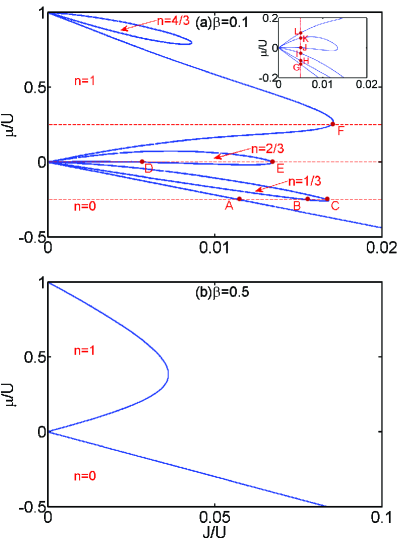
Figure 2: The ground-state phase diagram for the bosonic trimerized Kagomé lattice with different values of $\beta=J/T$: (a) $\beta=0.1$, (b) $\beta=0.5$. In our calculation, we choose the truncation number $N_{max}=8$. The insulator lobes with zero order parameters are surrounded by the superfluid phase with nonzero order parameters. In (a) (main panel), between neighboring integer insulator lobes, there appear exotic insulator loopholes with fractional filling numbers $n=k/3$ (where $k$ are positive integers). The inset in (a) is the magnification of the phase diagram for $\mu/U\in[-0.2,0.2]$.

If the hopping is dominated by the intra-trimer hopping (i.e. $\beta\ll 1$), there appears a new exotic phase, the FracI phase, which has zero order parameter $\Psi$ and fractional filling number $n$. In the strong hopping regime ($J/U\rightarrow\infty$), the GS is a superfluid. In the strong interaction regime ($J/U\rightarrow 0$), dependent on the chemical potential $\mu$ and the ratio $J/U$, the GS is a superfluid, an IntI or a FracI. As both integer and fractional insulators have zero order parameter, one has to calculate the filling number to distinguish them. In our bosonic TKL, the filling number of the FracI is multiplies of one third. Moreover, in the FracI phase, the particles can still move freely in the same cluster although they can not move between different clusters. In the phase diagram, the FracI phases appear as loopholes between neighboring IntI lobes. In addition, the loophole domains are obtained in the bosonic TKL by cell strong-coupling perturbation techniqueBuonsante et al. (2005), which solves the intra-trimer Hamiltonians exactly and treats the inter-trimer hopping as perturbation.

In Fig. 2(a), we show the phase diagram for the system of $\beta=0.1$. In the main panel of Fig. 2(a), the three red-dashed lines are parallel to the $J/U$ axis corresponding to $\mu/U=-0.25$, $0$, and $0.25$, respectively. Along the line of $\mu/U=-0.25$, the system undergoes the vacuum-superfluid-FracI-superfluid transition with three critical points (A, B, C) at $J/U=(0.01142,0.01528,0.01670)$. Along the line of $\mu/U=0$, the system undergoes the superfluid-FracI-superfluid transition with two critical points (D, E) at $J/U=(0.00548,0.01340)$. Along the line of $\mu/U=0.25$, the system undergoes the IntI-superfluid transition with the critical F at $J/U=0.01702$. We show in the inset the magnification of the phase diagram depicted in the main panel. The dashed line is parallel to the $\mu/U$ axis corresponding to $J/U=0.005$. Along this line, the system undergoes the vacuum-superfluid-FracI-superfluid-FracI-superfluid-IntI transition with the six critical points labeled as (G,H,I,J,K,L) at $\mu/U=(-0.111,-0.087,-0.037,0.001,0.065,0.099)$. The phase transitions along such lines, which are driven by the ratio $\mu/U$ or $J/U$ at variable filling, belong to the class of commensurate-incommensurate (CI) transitions. In addition to the CI transitions, there is another typical class of phase transitions in the BH systems, the O(2) transitions, which are driven by the ratio $J/U$ at fixed integer filling.

IV entanglement entropy and phase transitions

Now we show how to extract the signature of EE for QPTs in our bosonic TKL. As mentioned above, the Rényi EE is a bipartite entanglement defined through separating the whole system into two subsystems and its second-order form can be measured in experiments. Denoting the two subsystems as A and B, the $n$-th order Rényi EE is defined as

$$S_{n}[\mathrm{A}(\mathrm{B})]=\frac{1}{1-n}\log\mathrm{Tr}(\hat{\rho}_{\mathrm{A}(\mathrm{B})}^{n}).$$ (11)

Here, $\hat{\rho}_{\mathrm{A}(\mathrm{B})}=\mathrm{Tr}_{\mathrm{B}(\mathrm{A})}(\hat{\rho}_{\mathrm{AB}})$ is the reduced density matrix of subsystem $\mathrm{A}(\mathrm{B})$ and $\hat{\rho}_{\mathrm{AB}}$ is the density matrix of the whole system. If the two subsystems are entangled, ignoring information about one subsystem will result in the other subsystem being in a mixed quantum state. Through implementing the L’H$\hat{o}$pital’s rule, it is easy to find that the first-order Rényi EE just gives the von Neumann entropy. Below we concentrate on the second-order ($n=2$) Rényi EE, $S_{2}[\mathrm{A}(\mathrm{B})]=-\log\mathrm{Tr}(\hat{\rho}_{\mathrm{A}(\mathrm{B})}^{2})$.

In our cluster MF treatment, only the intra-cluster correlations are reserved, thus we only need to consider intra-cluster bipartite entanglement. For a given trimer-cluster R, the subsystem A can be chosen as one of the three sites and the subsystem B are then the rest two sites. Therefore, the reduced density matrices read as

$$\hat{\rho}_{\mathrm{A}(\mathrm{B})}=\mathrm{Tr}_{jk(i)}\hat{\rho}_{\mathrm{R}},$$ (12)

where $\{i,j,k\}$ label the three sites in cluster R. From the single-cluster GS Eq. (10), the reduced density matrix $\hat{\rho}_{A}$ and $\hat{\rho}_{B}$ are given as

$$\hat{\rho}_{\mathrm{A}} = \sum_{\begin{subarray}{c}n_{1},n^{\prime}_{1}\end{subarray}}\left(\sum_{n_{2},n_{3}}C_{n_{1}n_{2}n_{3}}C_{n^{\prime}_{1}n_{2}n_{3}}^{*}\right)\left|{n_{1}}\right\rangle\left\langle{n^{\prime}_{1}}\right|,$$

$$\hat{\rho}_{\mathrm{B}} = \sum_{\begin{subarray}{c}n_{2},n_{3}\\ n^{\prime}_{2},n^{\prime}_{3}\end{subarray}}\left(\sum_{n_{1}}C_{n_{1}n_{2}n_{3}}C_{n_{1}n^{\prime}_{2}n^{\prime}_{3}}^{*}\right)\left|{n_{2}n_{3}}\right\rangle\left\langle{n^{\prime}_{2}n^{\prime}_{3}}\right|.$$ (13)

According to the above reduced density matrices, we calculate the 2nd-order Rényi EE for different parameters. Our results show that, the second-order Rényi EE itself is continuous everywhere, but the continuousness of its first-order derivative breaks down at the phase boundary. This means that the QPTs in our bosonic TKL correspond to the jumps in the first-order derivative of the second-order Rényi EE.

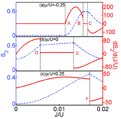
Figure 3: (color online). The second-order Rényi entanglement entropy $S_{2}$ and its first-order derivative with respect to $J/U$ for different values of $\mu/U$: (a) $-0.25$, (b) $0$, and (c) $0.25$. The blue-dot-and-dash and red lines denote $S_{2}(A)$ and $dS_{2}/d(J/U)$, respectively. The vertical black-dashed lines $\{\mathrm{A,B,C,D,E,F}\}$, where the derivative $dS_{2}/d(J/U)$ jumps, correspond to the transition points $\{\mathrm{A,B,C,D,E,F}\}$ in the main panel in Fig. 2(a).

In Fig. 3, corresponding to the three red-dashed lines in the main panel of Fig. 2(a), we show the second-order Rényi EE $S_{2}$ (blue-dot-and-dash lines) and its first-order derivative with respect to $J/U$ (red lines). The second-order Rényi EE is continuous everywhere but turnpoints appear at the phase boundary. To characterize the turnpoints, we numerically calculate its first-order derivative with respect to $J/U$ through difference quotient. Indeed, the first-order derivatives (red lines) show discontinuousness at the phase boundaries (vertical black-dashed lines). The three vertical black-dashed lines (A, B, C) correspond to the critical points of the vacuum-superfluid-FracI-superfluid transition, see Fig. 3(a). The two vertical black-dashed lines (D, E) correspond to the critical points of the superfluid-FracI-superfluid transition, see Fig. 3(b). The vertical black-dashed line F corresponds to the critical point of the IntI-superfluid transition, see Fig. 3(c). Similarly, the first-order derivative of $S_{2}$ with respect to $\mu/U$ also shows discontinuousness at the phase boundary, see Fig. 4.

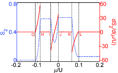
Figure 4: (color online). The second-order Rényi entanglement entropy $S_{2}(A)$ and its first-order derivative with respect to $\mu/U$ for $J/U=0.005$. The blue-dot-and-dash and red lines denote $S_{2}$ and $dS_{2}/d(\mu/U)$, respectively. The vertical black-dashed lines $\{\mathrm{G,H,I,J,K,L}\}$, where the derivative $dS_{2}/d(J/U)$ jumps, correspond to the transition points $\{\mathrm{G,H,I,J,K,L}\}$ in the inset in Fig. 2(a).

The above analysis is based on the class of CI transition. By employing the slave-boson approach, it has been demonstrated that the von Neumann EE develops cusp singularities at the SI transition in a square BH lattice Frérot and Roscilde (2016), which is a CI transition. Due to that the “Higgs”-like modes are gapless at the O(2) transitions while they are gapped at the CI transitions, it has been found that the singularities at the O(2) transitions are greatly enhanced Frérot and Roscilde (2016). So, we believe that our findings may apply to the O(2) transitions as well.

V experimental possibility

Based upon the present techniques of manipulating and detecting ultracold atoms in optical lattices, it is possible to realize our bosonic TKL and measure its second-order Rényi EE. By imposing three standing-wave lasers, the Kagomé optical lattice has been realized and our bosonic TKL can be realized by loading ultracold Bose atoms in the the Kagomé optical lattice Jo et al. (2012). Based upon the quantum interference between many-body twins Daley et al. (2012), the experimental measurement of the second-order Rényi EE has been demonstrated by using simple BH systems Islam et al. (2015). Similarly, the second-order Rényi EE in our bosonic TKL can be measured through three steps: state initialization, quantum interference and parity readout.

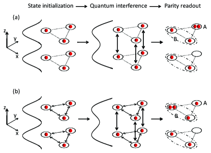
Figure 5: (color online). Schematic diagram for measuring the second-order Rényi entanglement entropy in our bosonic TKL via quantum interference of many-body twins. The cluster (a trimer) is divided into two subsystems A and B. The measurement procedure includes three steps: state initialization, quantum interference and parity readout. (a) For a product state of the two subsystems, which has zero second-order Rényi EE, the final particle numbers of the subsystems and the whole system are even. (b) For an entangled state of the two subsystems, which has nonzero second-order Rényi EE, the final particle numbers in the subsystems are even or odd while they are even in the whole system.

The schematic diagram for the measurement is shown in Fig. 5. Firstly, prepare two identical clusters in two decoupled parallel TKLs and initialize them into the same state. This can be achieved by superimposing a box potential onto a three-dimensional TKL to decouple a bilayer TKL Jo et al. (2012) and then applying a proper double-well potential to decouple two identical clusters in different layers. Secondly, perform a discrete Fourier transformation on the two copies. This can be realized by the beam-splitter operation through lowing the potential barrier between the two layers, in which the bosons in different layers interfere through inter-layer quantum tunneling. Finally, read out the number of particles in one copy and its subsystems through site-resolved readout. From the measured total particle number in subsystem A, $n_{\mathrm{A}}=\sum_{i\in\mathrm{A}}n_{i}$, one can obtain the purity $\mathrm{Tr}(\rho_{\mathrm{A}}^{2})=\langle(-1)^{n_{\mathrm{A}}}\rangle$, which is just the average measured parity $P_{\mathrm{A}}=(-1)^{n_{\mathrm{A}}}$. Through the parity measurement of subsystem A, the second-order Rényi EE is given as $S_{2}(\mathrm{A})=-\log\mathrm{Tr}(\rho_{\mathrm{A}}^{2})=-\log{\langle(-1)^{n_{\mathrm{A}}}\rangle}$. Thus, $S_{2}$ is zero if A and B are not entangled and nonzero if A and B are entangled.

VI conclusion and discussion

In summary, based upon the cluster MF treatment, we have successfully extract the signature of second-order Rényi EE for the QPTs of interacting bosons in TKL. In addition to the superfluid and integer insulator phases, we find that fractional insulator phase may appear in strongly trimerized systems. Through analyzing the second-order Rényi EE and its first-order derivative, we explore that, while the second-order Rényi EE itself is continuous everywhere, its first-order derivative becomes discontinuous at the quantum critical points. This means that the intra-cluster entanglement reserved in the cluster MF treatment is still sufficient for capturing the signature of EE in QPTs.

Our method for extracting the residual intra-cluster entanglement provides a highly efficient and rapid way to capture the signature of EE for the QPTs in quantum superlattice models. In comparison with the TEBD, DMRG and QMC methods Lauchli and Kollath (2008); Pino et al. (2012); Alba et al. (2013); Isakov et al. (2011), which cost huge computational resources and long computational times, the calculation of EE via the cluster MF treatment costs much less computational resources and short computational time. In comparison with the exact diagonalization Buonsante and Vezzani (2007), which can only give phase crossovers, the calculation of EE via the cluster MF treatment may explore true phase transitions. As the cluster MF approach is a powerful tool for exploring most QPTs in various many-body quantum models (from Fermi-Hubbard model, Bose-Hubbard model to Heisenberg spin model) with different superlattice configurations (from double-well latticesSebby-Strabley et al. (2006); Chen et al. (2011); Atala et al. (2014); Tokuno and Georges (2014); Keleş and Oktel (2015); Deng et al. (2015), Kagomé latticesMielke (1992); Santos et al. (2004); Damski et al. (2005); Jo et al. (2012); Pudleiner and Mielke (2015) to honeycomb latticesGrynberg et al. (1993); Snoek and Hofstetter (2007); Lee et al. (2009); Lembessis et al. (2015)), beyond extracting the signature of EE for bosonic SI transitions, we believe that our analysis can be easily extended to extract the signature of EE for other QPTs in quantum superlattice systems.

We also note that the cluster dynamical mean-field approach (CDMFA) has been employed to study the entanglement spectrum of the half-filling Hubbard system Udagawa2015 . Although both the cluster mean-field approach (CMFA) and the CDMFA can be used to decouple many-body lattice model into many-body cluster model, they are different. The CDMFA based upon the dynamical mean-field theory freezes spatial fluctuations but takes full account of local temporal fluctuations. The CMFA we use here takes into account first-order spatial fluctuations but ignores temporal fluctuations.