High-Roller Impact: A Large Generalized Game Model of Parimutuel Wagering

Abstract.

How do large-scale participants in parimutuel wagering events affect the house and ordinary bettors? A standard narrative suggests that they may temporarily benefit the former at the expense of the latter. To approach this problem, we begin by developing a model based on the theory of large generalized games. Constrained only by their budgets, a continuum of diffuse (ordinary) players and a single atomic (large-scale) player simultaneously wager to maximize their expected profits according to their individual beliefs. Our main theoretical result gives necessary and sufficient conditions for the existence and uniqueness of a pure-strategy Nash equilibrium. Using this framework, we analyze our question in concrete scenarios. First, we study a situation in which both predicted effects are observed. Neither is always observed in our remaining examples, suggesting the need for a more nuanced view of large-scale participants.

1. Introduction

Suppose that a collection of bettors are wagering on an upcoming event. The payoffs are determined via a (frictionless) parimutuel system if whenever Outcome $i$ occurs, Bettor $A$ receives

$$\left(\text{Total Amount Wagered}\right)\left(\frac{\text{Bettor $A$'s Wager on Outcome $i$}}{\text{Total Amount Wagered on Outcome $i$}}\right).$$

The idea is that players with correct predictions will proportionally share the final betting pool. Prizes are reduced in practice by transaction costs such as the house take, a percentage fee collected by the betting organizer (or house). For example, Bettor $A$ might only win

$$\kappa\left(\text{Total Amount Wagered}\right)\left(\frac{\text{Bettor $A$'s Wager on Outcome $i$}}{\text{Total Amount Wagered on Outcome $i$}}\right)$$ (1.1)

when Outcome $i$ occurs, if the house take is $\left(1-\kappa\right)\%$ for some $0<\kappa<1$.

This mechanism was invented in the context of horse race gambling by Oller in the late 1800’s ([10]) and remains widely employed in that setting: In 2014, worldwide parimutuel betting on horse races totaled around seventy-five billion euros ([2]). It also typically determines wagering payoffs for other sports such as jai alai and races involving bicycles, motorcycles, motorboats, and greyhounds ([7]). Certain prizes for major lotteries such as Mega Millions, Powerball, and “EuroMillions” are computed in a parimutuel fashion ([1]). Parimutuel systems are increasingly popular methods for distributing payoffs in online prediction markets as well ([42]). Goldman Sachs Group, Inc., Deutsche Bank AG, CME Group Inc., Deutsche Börse AG, and ICAP have even facilitated the development of parimutuel derivatives on economic indicators ([7]).

The first scholarly publication on parimutuel wagering was written by Borel in 1938 ([9]), and more recent surveys and anthologies ([51]; [22]; [21]) attest to the substantial academic interest garnered by this topic since. A vast range of issues from optimal betting ([28]; [48]; [8]) to market efficiency ([23]; [3]; [27]) to market microstructure ([33]; [42]; [41]) has been extensively studied. Significant attention has been paid to strategic interactions among bettors ([45]; [40]; [31]; [50]; [43]).

Similar to the rise of high-frequency and algorithmic traders in financial markets, a growing number of parimutuel wagering event participants are organizations employing large-scale strategies based upon advanced mathematical, statistical, and computational techniques ([30]). There are fundamental differences between these bettors and more traditional wagerers. The new firms typically have access to vast budgets, making their betting totals orders of magnitude beyond the amounts wagered by regular players. Often, they can place their wagers at speeds impossible for ordinary bettors to match. Presumably, their use of complex methods also makes their forecasts and corresponding wagering strategies generally superior.

The house collects a percentage of the total amount wagered and, therefore, may initially benefit from the presence of large-scale wagering firms. After all, their activities should increase the size of the pool, at first anyway. The factors just described are thought to put ordinary bettors at an extreme disadvantage, though. Since payouts are calculated according to (1.1), ordinary bettors’ profits may even directly decline as a result of the large-scale firms’ wagers. If this discourages enough regular players from betting, then pool sizes may eventually dwindle, hurting the house’s revenue. In fact, many betting organizers have publicly expressed strong concerns about the new breed of wagerers. Betting organizers have even occasionally banned these participants from parimutuel wagering events ([30]).

How reasonable is this narrative? Our goal is to quantify the impact of large-scale participants in parimutuel wagering events on the house and ordinary bettors.

First, using the theory of large generalized games, i.e., games with a continuum of diffuse (or non-atomic/minor) players and finitely many atomic (or major) players, we develop a model of parimutuel betting. The bets made by individual atomic players affect all others because they change the final payoff per unit bet on Outcome $i$:

$$\kappa\left(\frac{\text{Total Amount Wagered}}{\text{Total Amount Wagered on Outcome $i$}}\right).$$ (1.2)

Aggregate decisions made by the diffuse players also affect every player for the same reason. A key feature is that an individual diffuse player cannot change (1.2) by revising her wagers. In fact, her specific choices have no effect whatsoever on the rest of the game’s participants.

We view diffuse and atomic players as stand-ins for ordinary bettors and large-scale wagering firms, respectively. The approximation is motivated by the observation that the total amount wagered by a single traditional bettor is generally negligible compared to the total amount wagered by an entire betting firm.

Our main theoretical result, Theorem 4.3, provides necessary and sufficient conditions for the existence and uniqueness of a pure-strategy Nash equilibrium. Other scholars have shown the existence of equilibria in a broad class of large generalized games ([5]; [6]; [11]; [46]). Such results often rely upon sophisticated technology including variants of the Kakutani fixed-point theorem. We choose to employ a more elementary fixed-point argument instead. Advantages of our approach include its simplicity and the possibility of proving the equilibrium’s uniqueness. A simple algorithm for computing relevant equilibrium quantities immediately presents itself as well.

Having such an algorithm allows us to analyze our problem in specific scenarios. In accordance with the prevailing narrative, we observe that because of the atomic player, the house is temporarily better off and the diffuse players are worse off in Example 5.2. For varying reasons, at least one of these effects is not observed in each of the remaining situations.

In Example 5.3, the diffuse players are better off in the presence of the atomic player. Intuitively, when the event is too close to call, the atomic player can bet on the wrong outcome even if her prediction is assumed to be quite accurate. Such an error is to the advantage of the diffuse players.

In Example 5.4, the diffuse players believe that they are better off when there is an atomic player. Roughly, if the diffuse players’ beliefs are too homogeneous but the atomic player disagrees with them, the diffuse players’ expected profits per unit bet rise when the atomic player takes the other side of their wagers.

In Example 5.5, we argue that the diffuse players are better off but the house is (immediately) worse off because of the atomic player, exactly the opposite of the prevailing narrative. To make this point, we recast our model as a two-stage game taking into account the house’s strategic decisions. Effectively, because the atomic player considers her impact on (1.2), she has a lower tolerance for unfavorable betting conditions than the diffuse player. When she is absent, this means that the house can more easily prey upon the diffuse players.

Before offering further details, we more thoroughly discuss related literature in Section 2. We carefully present our model in Section 3 and our main theoretical result in Section 4. We numerically investigate our concrete examples in Section 5. Appendix A highlights a few technical aspects of Section 4’s work. We give our longer formal proofs in Appendices B and C.

2. Related Literature

The individual states of our diffuse players are only coupled via the empirical distribution of controls. Since each diffuse player is too small to influence this distribution, she treats it as fixed when determining her own strategy. Assumptions like these have appeared in the literature on continuum games ([4]; [49]; [35]; [47]) and mean-field games ([34]; [26]).

Our paper bears a stronger resemblance to work in the former category. For instance, we model parimutuel wagering as a static game. Such a choice is quite common in a continuum game study; however, stochastic differential games are more often the focus in mean-field game theory. Also, we restrict ourselves to an intuitive argument for viewing ordinary bettors as diffuse players. Papers on mean-field games often rigorously present their continuum model as a limit of finite population models, while those on continuum games typically emphasize other issues.

General mean-field interactions among players can be described by complex functions of the empirical distributions of states and/or controls. On the other hand, parimutuel wagerers affect one another through (1.2) alone, a comparatively simple scenario. This makes parimutuel wagering an especially strong candidate for modeling by either theory. Continuum games have already been applied in this way ([38]; [54]).

Watanabe considered a two-stage game with a betting organizer and a continuum of risk-neutral diffuse players with heterogeneous beliefs ([54]). First, the betting organizer selects a value for the house take. The diffuse players then determine whether to place a unit bet on one of two outcomes or bet nothing at all. Using techniques from set-valued analysis, Watanabe showed that an equilibrium always exists, provided the house take is not too large. As long as each player can only bet negligible amounts, Watanabe also found that equilibria in parimutuel wagering games are regular. That is, if a player wagering on Outcome $i$ believes that Outcome $i$ will occur with probability $p$, all players who believe that Outcome $i$ will occur with probability $p^{\prime}>p$ also wager on Outcome $i$. The paper’s results on the betting organizer’s optimal strategy were in the context of specific examples.

Ottaviani and Sørenson developed their continuum game to explain two phenomena frequently observed in the context of parimutuel wagering on horse races: late informed betting and the favorite-longshot bias ([38]). The first states that more accurate information about a race’s outcome can be gleaned from late bets than early bets. The second says that the public tends to excessively bet on unlikely outcomes and wager too little on likely outcomes. A continuum of privately informed risk-neutral players decide when to place their individual bets in a discrete-time setting. They can wager a unit amount on one of two outcomes or abstain from betting. The paper gave conditions under which all of these players simultaneously wager at the terminal time, and the corresponding equilibrium is shown to always feature the favorite-longshot bias.

Others have more implicitly created infinite-player parimutuel wagering models by assuming that there are many bettors ([27]; [39]). These references have sought to identify other possible causes of the favorite-longshot bias.

The most important new feature of our setup is that, in addition to the diffuse bettors, we introduce an atomic bettor. The parimutuel wagering studies we just discussed only incorporate diffuse players. We would not be able to understand the effects of large-scale wagering organizations on ordinary bettors, if we made a similar assumption.

Because of this addition, our model belongs to the class of continuum game models known as large generalized games. Games that include both diffuse and atomic players can be found in mean-field game theory as well under the heading major-minor player models ([25]; [36]; [37]; [29]; [53]). Applications of large generalized games are known to be diverse and already include a collection of problems from politics ([17]) to oligopolistic markets ([57]). General results on the existence of equilibria in large generalized games have also been obtained ([5]; [6]; [11]; [46]). We choose not to rely upon these, as the simple structural aspects of parimutuel wagering just discussed, combined with a convenient modeling assumption (see Section 3), allow us to use elementary arguments.

Ultimately, we employ a mean-field approximation for the standard reason: By doing so, we make our model tractable, hopefully while preserving the critical macroscopic properties of our original problem. Issues other than the impact of large-scale wagering organizations have been resolved in finite-player settings, though such studies have usually invoked other strong assumptions.

Weber gave sufficient conditions for the existence of an equilibrium in a simultaneous parimutuel betting game with $N$ atomic players, each of whom is risk-neutral and must bet a specific total amount ([56]). Watanabe, Nonoyama, and Mori’s setup and goals are similar to those in Watanabe’s continuum game paper, except that the diffuse players in the latter are replaced by finitely many atomic players ([55]; [54]). Explanations of the favorite-longshot bias have been offered using equilibrium results for $N$-player parimutuel wagering games ([13]; [31]; [40]; [44]). Games in which finitely many bettors wager sequentially have also been investigated for various purposes ([18]; [16]; [32]; [31]; [52]). For example, Thrall showed that if risk-neutral atomic bettors with homogeneous beliefs wager sequentially, their profits tend to zero as the number of bettors increases ([52]). Note that some of these works do consider limiting cases in which the population of wagerers grows arbitrarily large to complement their other insights ([52]; [40]).

3. Model Details

Our players have the opportunity to wager on an event that can unfold in two mutually exclusive ways: Outcome 1 might occur. If not, Outcome 2 will occur. For now, we view $\kappa\in\left(0,1\right)$ to be exogenously given. Inspired by Watanabe et al. ([55]; [54]), we later informally consider what happens when we allow the house take to be optimally selected by the betting organizer in the first stage of a two-stage game (see Example 5.5). Our results in Section 4 are unaffected by such a shift.

The unit interval describes the diffuse bettors’ views on the likelihood of Outcome 1: the bettors whose views are indexed by $p\in\left[0,1\right]$ believes that Outcome 1 will occur with probability $p$. Initially, each diffuse bettor has some (negligible) unit wealth. A finite Borel measure $\mu$ with a continuous everywhere positive density characterizes the distribution of the diffuse bettors. More precisely, the total initial wealth of all diffuse bettors whose views are contained in a Borel set $A$ is $\mu\left(A\right)$.

That $\mu$ has a continuous everywhere positive density is our convenient modeling assumption from Section 2. It is similar to a key hypothesis in Ottaviani and Sørenson’s work, although the posterior beliefs of their diffuse bettors are obtained after updating a common prior belief using a private signal and Bayes’ rule ([38]). Effectively, Watanabe assumed that $\mu$ need not have a density, and even when it does, the density need not be positive everywhere ([54]). These choices necessitated a set-valued approach, which we are able to avoid.

Continuity merely simplifies a few of our arguments, e.g., see Step C of Theorem 4.3’s proof. The rest of the assumption plays a more critical role. Results on the existence of equilibria in parimutuel wagering games often include a hypothesis such as the following: for any given outcome, at least two bettors believe that the outcome will occur with positive probability. By supposing that the density is positive, we assume this as well. Watanabe has shown that an equilibrium may not be unique, if $\mu\left(\left\{p\right\}\right)>0$ for some fixed $p$ ([54]). Obviously, this situation is prevented by the density’s existence.

Our atomic player believes that Outcome 1 will occur with probability $q\in\left[0,1\right]$. She has (non-negligible) finite initial wealth $w>0$.

Throughout, we treat all players’ beliefs as exogenously determined. We do not address how the players generate their estimates; however, this process is of great interest both practically and academically ([22]; [21]). For our theoretical results in Section 4, we also do not specify how the players’ estimates compare to the actual probability that Outcome 1 will occur. Since large-scale betting organization allegedly produce highly accurate forecasts, we could choose $q$ to be some small perturbation of the actual probability of Outcome 1. We informally experiment with this extra assumption in Examples 5.2 and 5.3.

All players decide how much to wager on each outcome. Their choices are constrained only by their initial wealth: a betting strategy is feasible (or admissible) for an individual bettor as long as the sum of her wagers is no more than her wealth. For example, a bettor could choose to wager 100% of her wealth on Outcome 1, 55% of her wealth on Outcome 1 and 30% of her wealth on Outcome 2, or not wager at all. We formalize this as follows.

Definition 3.1.

A feasible strategy profile for the diffuse players is a measurable function

$$f=\left(f_{1},f_{2}\right):\left(0,1\right)\longrightarrow\left\{\left(x_{1},x_{2}\right)\in\mathbb{R}^{2}_{\geq 0}\,:\,x_{1}+x_{2}\leq 1\right\}.$$

A feasible strategy profile for the atomic player is a vector $a=\left(a_{1},a_{2}\right)\in\mathbb{R}^{2}_{\geq 0}$ such that

$$a_{1}+a_{2}\leq w.$$

We call the pair $\left(f,a\right)$ a feasible strategy profile.

Under $\left(f,a\right)$, the atomic player wagers $a_{i}$ on Outcome $i$. Each diffuse player who believes that Outcome 1 will occur with probability $p$ wagers $f_{i}\left(p\right)\times 100\%$ of her (negligible) unit initial wealth on Outcome $i$.

Our space of feasible strategy profiles is slightly atypical. Previously, diffuse players in parimutuel wagering games have only been able to place unit bets, if they bet at all ([38]; [54]). We could have made this restriction as well without loss of generality due to Proposition 4.1. Watanabe allowed groups of diffuse players to wager differently, even if they held identical beliefs ([54]). In equilibrium, such a discrepancy could only arise among the diffuse players who believed that their expected profits would be zero. We encounter a related ambiguity in our framework (see our discussion of Proposition 4.1). For us, the $\mu$-measure of this set of bettors is zero, and we anticipate that all of our main results would remain the same, if we were to relax the diffuse bettors’ same beliefs-same bets restriction. More significantly, atomic players have been frequently constrained to wager a fixed amount in total or a unit amount on a single outcome when they bet ([56]; [55]; [13]; [40]). Proposition 4.2 suggests that imposing these restrictions would have a severe effect.

The total amount that the diffuse players wager on Outcome $i$, denoted $d_{i}$, is given by

$$d_{i}=\displaystyle\int_{0}^{1}f_{i}\left(p\right)\mu\left(dp\right).$$

Since $\mu$ has a density, we immediately confirm that the bets placed by any given diffuse player are too small to affect the amount wagered on any specific outcome. Of course, if she revises her strategy, then a particular diffuse player affects neither the total amount wagered nor (1.2). All of these quantities could change when aggregations of diffuse players, that is, collections of diffuse players whose beliefs are contained in a Borel set $A$ with positive $\mu$-measure, revise their wagers.

Payoffs are determined according to (1.1). Each player selects her wagering strategy simultaneously in order to maximize her expected profit according to her beliefs. We implicitly assume that every bettor knows $\kappa$, $\mu$, $q$, and $w$, so that she can select the best response to her opponents’ collective actions. Similar assumptions can be found in many other equilibrium studies on parimutuel wagering ([56]; [55]; [54]; [13]; [40]).

Since each diffuse player starts out with negligible unit wealth, technically, we should only discuss the expected profits of diffuse bettors whose views lie in some Borel set $A$. We nevertheless compute and refer to the expected profits of an individual diffuse bettor in an obvious, but admittedly informal, way. Doing so helps motivate our definition of a pure-strategy Nash equilibrium (see Definition 3.3) and highlight the intuition underlying our results.

A seemingly more formidable concern is how to handle (1.1) in pathological cases. It is trivial to produce a feasible strategy profile $\left(f,a\right)$ such that for some $p$, we have $f_{j}\left(p\right)>0$ but

$$d_{j}=a_{j}=0.$$

Naïvely translating (1.1), we conclude that a diffuse player whose views are indexed by $p$ receives

$$\kappa\left(\displaystyle\sum_{i=1}^{2}\left(d_{i}+a_{i}\right)\right)\left(\displaystyle\frac{f_{j}\left(p\right)}{d_{j}+a_{j}}\right)$$ (3.1)

whenever Outcome $j$ occurs.

If

$$d_{1}=d_{2}=a_{1}=a_{2}=0,$$

then the total amount wagered is zero. Practically, the betting organizer would probably cancel such an event, which suggests that it is natural to set all players’ payoffs to zero in this scenario.

Alternatively, we might have

$$d_{i}+a_{i}>0$$

for $i\neq j$. There are now two appealing options for the diffuse player’s payoff. First, we might choose to set the payoff to zero. Practically, no bettor would receive a payout, if Outcome $j$ occurred but no one wagered on it. We also might set the payoff to $+\infty$, as in Watanabe’s work ([54]). In practice, if the amount wagered on Outcome $j$ were zero, each player who believed that Outcome $j$ would occur with positive probability would want to place an arbitrarily small bet on Outcome $j$. Setting the payoff to $+\infty$ captures this intuition.

We choose the first option, but selecting the second instead would not change our results. Only equilibrium payoffs need to be computed, and in an equilibrium, positive amounts are always wagered on both outcomes. Essentially, the scenario we describe never arises. One reason is that we do not allow the trivial (or null) equilibrium in which no player wagers. We could, but as Watanabe observed, that case is comparatively uninteresting and practically unimportant ([54]). Roughly, the other reason is the same as our justification for possibly setting the payoff to $+\infty$.

Before making this discussion precise, we introduce some notation.

Definition 3.2.

Given a feasible strategy profile $\left(f,a\right)$ such that at least one of the $d_{i}$’s or $a_{i}$’s is positive, the implied (or subjective) probability that Outcome 1 will occur, denoted $P^{f,a}$, is defined by

$$P^{f,a}=\displaystyle\frac{d_{1}+a_{1}}{\sum_{i=1}^{2}\left(d_{i}+a_{i}\right)}.$$

We refer to

$$1-P^{f,a}=\displaystyle\frac{d_{2}+a_{2}}{\sum_{i=1}^{2}\left(d_{i}+a_{i}\right)}$$

as the implied (or subjective) probability that Outcome 2 will occur.

$P^{f,a}$ is the ratio of the amount wagered on Outcome 1 to the total amount wagered, assuming the latter is positive. Our previous discussion implies that $P^{f,a}\in\left(0,1\right)$ in equilibrium. Since the argument was informal, we do not yet take this as fact. In particular, the amount received by a diffuse player who believes that Outcome 1 will occur with probability $p$ is

$$\kappa\left(\displaystyle\sum_{i=1}^{2}\left(d_{i}+a_{i}\right)\right)\left(\displaystyle\frac{f_{1}\left(p\right)\mathds{1}_{\left\{d_{1}+a_{1}\neq 0\right\}}}{d_{1}+a_{1}}\right)=\displaystyle\frac{\kappa f_{1}\left(p\right)\mathds{1}_{\left\{P^{f,a}\neq 0\right\}}}{P^{f,a}}$$

and

$$\kappa\left(\displaystyle\sum_{i=1}^{2}\left(d_{i}+a_{i}\right)\right)\left(\displaystyle\frac{f_{2}\left(p\right)\mathds{1}_{\left\{d_{2}+a_{2}\neq 0\right\}}}{d_{2}+a_{2}}\right)=\displaystyle\frac{\kappa f_{2}\left(p\right)\mathds{1}_{\left\{P^{f,a}\neq 1\right\}}}{1-P^{f,a}}$$

when Outcomes 1 and 2 occur, respectively. Hence, this diffuse player believes that her expected profit is

$$f_{1}\left(p\right)\left(\displaystyle\frac{\kappa\,\mathds{1}_{\left\{P^{f,a}\neq 0\right\}}\,p}{P^{f,a}}-1\right)+f_{2}\left(p\right)\left(\displaystyle\frac{\kappa\,\mathds{1}_{\left\{P^{f,a}\neq 1\right\}}\,\left(1-p\right)}{1-P^{f,a}}-1\right).$$ (3.2)

Similarly, the atomic player thinks that her expected profit is

$$a_{1}\left(\displaystyle\frac{\kappa\,\mathds{1}_{\left\{P^{f,a}\neq 0\right\}}\,q}{P^{f,a}}-1\right)+a_{2}\left(\displaystyle\frac{\kappa\,\mathds{1}_{\left\{P^{f,a}\neq 1\right\}}\,\left(1-q\right)}{1-P^{f,a}}-1\right).$$ (3.3)

Definition 3.3.

A pure-strategy Nash equilibrium is a feasible strategy profile $\left(f^{\star},a^{\star}\right)$ such that

1. at least one of the $d_{i}^{\star}$’s or $a_{i}^{\star}$’s is positive;

2. for any $p\in\left[0,1\right]$,

   $$f_{1}^{\star}\left(p\right)\left(\displaystyle\frac{\kappa\,\mathds{1}_{\left\{P^{f^{\star},a^{\star}}\neq 0\right\}}\,p}{P^{f^{\star},a^{\star}}}-1\right)+f_{2}^{\star}\left(p\right)\left(\displaystyle\frac{\kappa\,\mathds{1}_{\left\{P^{f^{\star},a^{\star}}\neq 1\right\}}\,\left(1-p\right)}{1-P^{f^{\star},a^{\star}}}-1\right)$$

   $$\quad=\displaystyle\sup_{\begin{subarray}{c}b_{1},b_{2}\geq 0\\ b_{1}+b_{2}\leq 1\end{subarray}}\left\{b_{1}\left(\displaystyle\frac{\kappa\,\mathds{1}_{\left\{P^{f^{\star},a^{\star}}\neq 0\right\}}\,p}{P^{f^{\star},a^{\star}}}-1\right)+b_{2}\left(\displaystyle\frac{\kappa\,\mathds{1}_{\left\{P^{f^{\star},a^{\star}}\neq 1\right\}}\,\left(1-p\right)}{1-P^{f^{\star},a^{\star}}}-1\right)\right\};$$

3. and

   $$a_{1}^{\star}\left(\displaystyle\frac{\kappa\,\mathds{1}_{\left\{P^{f^{\star},a^{\star}}\neq 0\right\}}\,q}{P^{f^{\star},a^{\star}}}-1\right)+a_{2}^{\star}\left(\displaystyle\frac{\kappa\,\mathds{1}_{\left\{P^{f^{\star},a^{\star}}\neq 1\right\}}\,\left(1-q\right)}{1-P^{f^{\star},a^{\star}}}-1\right)$$

   $$\quad=\displaystyle\sup_{\begin{subarray}{c}b_{1},b_{2}\geq 0\\ b_{1}+b_{2}\leq w\\ d_{1}^{\star},d_{2}^{\star},b_{1}\text{ or }b_{2}>0\end{subarray}}\left\{b_{1}\left(\displaystyle\frac{\kappa\,\mathds{1}_{\left\{P^{f^{\star},b}\neq 0\right\}}\,q}{P^{f^{\star},b}}-1\right)+b_{2}\left(\displaystyle\frac{\kappa\,\mathds{1}_{\left\{P^{f^{\star},b}\neq 1\right\}}\,\left(1-q\right)}{1-P^{f^{\star},b}}-1\right)\right\}.$$

(i) formally excludes the case in which the total amount wagered is zero. (ii) and (iii) ensure that each player maximizes her expected profit according to her beliefs, given her opponents’ wagers.

First, observe that each player requires very little information about her opponents’ strategies. For a given diffuse bettor, knowing $P^{f^{\star},a^{\star}}$ alone is enough. The atomic player must be able to compute $P^{f^{\star},b}$ for all of her feasible strategy profiles $b$, so it is sufficient for her to know $d_{1}^{\star}$ and $d_{2}^{\star}$. The difference for the two kinds of players reflects that an individual diffuse player cannot affect the implied probability of Outcome 1, while the atomic player can. These remarks explain why we informally claim that only the atomic player and aggregations of diffuse players affect the other participants. Notice that each player’s strategy depends anonymously on her opponents’ bets: how, specifically, her opponents wagers produced $P^{f^{\star},a^{\star}}$, $d_{1}^{\star}$, and $d_{2}^{\star}$ is irrelevant.

Although we only optimize over $b$ in (iii), the apparent possibility that $d_{1}^{\star}=d_{2}^{\star}=0$ motivates our use of the extra constraint

$$d_{1}^{\star},d_{2}^{\star},b_{1}\text{ or }b_{2}>0.$$

One might be concerned that we do not consider the feasible strategy $b_{1}=b_{2}=0$ for the atomic player, if $d_{1}^{\star}=d_{2}^{\star}=0$. Recall that all players receive a payoff of zero in such a situation. A simple calculation shows that the supremum is then also zero, so no issue is caused by our omission.

The last important concept for our modeling framework is uniqueness.

Definition 3.4.

A pure-strategy Nash equilibrium $\left(f^{\star},a^{\star}\right)$ is unique if for any other pure-strategy Nash equilibrium $\left(f^{\diamond},a^{\diamond}\right)$, we have $f^{\star}=f^{\diamond}$ $\mu$-a.s. and $a^{\star}=a^{\diamond}$.

We allow $f^{\star}$ and $f^{\diamond}$ to disagree on a set of $\mu$-measure zero since, ultimately, all relevant equilibrium quantities such as the implied probabilities are unaffected by such a difference. Soon, we see that $f^{\star}\left(p\right)$ and $f^{\diamond}\left(p\right)$ must be equal for all but two points, at most. There is only uncertainty about the behavior of the diffuse bettors who believe that their expected profits are zero (cf. our discussion about our space of feasible strategy profiles).

4. Theoretical Results

We now state and prove our theoretical results, beginning with Propositions 4.1 and 4.2. The former describes how the diffuse players should wager in response to the atomic player’s strategy. The latter tells us how the atomic player should bet, given the diffuse players’ wagers. We use these observations to prove Theorem 4.3, our main result. Recall that it offers necessary and sufficient conditions for the existence and uniqueness of a pure-strategy Nash equilibrium.

We conclude Section 4 with Corollaries 4.4, 4.5, and 4.6. Corollary 4.4 says that the atomic player wagers on a particular outcome if and only if the final expected profit per unit bet on that outcome is positive. The next corollary states that our equilibria are regular in a particular sense, while Corollary 4.6 says that the implied probability of Outcome 1 tends to $0.5$ uniformly as the house take approaches $50\%$.

Proposition 4.1.

Let $\left(f,a\right)$ be a feasible strategy profile such that $d_{1}$, $d_{2}>0$. $f$ satisfies

$$f_{1}\left(p\right)\left(\displaystyle\frac{\kappa\,p}{P^{f,a}}-1\right)+f_{2}\left(p\right)\left(\displaystyle\frac{\kappa\,\left(1-p\right)}{1-P^{f,a}}-1\right)$$

$$\quad=\displaystyle\sup_{\begin{subarray}{c}b_{1},b_{2}\geq 0\\ b_{1}+b_{2}\leq 1\end{subarray}}\left\{b_{1}\left(\displaystyle\frac{\kappa\,p}{P^{f,a}}-1\right)+b_{2}\left(\displaystyle\frac{\kappa\,\left(1-p\right)}{1-P^{f,a}}-1\right)\right\}$$ (4.1)

for all $p\in\left[0,1\right]$ if and only if

$$f_{1}\left(p\right) =\left\{\begin{array}[]{cc}1&\quad\text{if }\,\,p>P^{f,a}/\kappa\\ &\\ 0&\quad\text{if }\,\,p<P^{f,a}/\kappa\\ \end{array}\right.\qquad\qquad f_{2}\left(p\right)=\left\{\begin{array}[]{cc}1&\quad\text{if }\,\,1-p>\left(1-P^{f,a}\right)/\kappa\\ &\\ 0&\quad\text{if }\,\,1-p<\left(1-P^{f,a}\right)/\kappa\\ \end{array}\right..$$

First, notice that $P^{f,a}\in\left(0,1\right)$ since both $d_{1}$ and $d_{2}$ are positive. Comparing (4.1) and (ii) of Definition 3.3, we find that Proposition 4.1 provides a simple characterization of the diffuse players’ equilibrium strategies in this case, given the bets of the atomic player. Our assumption is not too restrictive, as Step C of Theorem 4.3’s proof says that $d_{1}$ and $d_{2}$ are always both positive in equilibrium.

Three distinct groups of diffuse bettors emerge: The first group, containing the diffuse bettors who believe that Outcome 1 will occur with probability greater than $P^{f,a}/\kappa$, wager all of their initial wealth on Outcome 1. Diffuse bettors who think that Outcome 2 will occur with probability greater than $\left(1-P^{f,a}\right)/\kappa$ make up the second group. These players bet their entire fortunes on Outcome 2. The remaining diffuse players, except those whose beliefs are indexed by $p=P^{f,a}/\kappa$ or $\left(1-P^{f,a}\right)/\kappa$, do not wager at all. None of the groups overlap, since $0<\kappa<1$ implies that

$$1-\left(\displaystyle\frac{1-P^{f,a}}{\kappa}\right)<\displaystyle\frac{P^{f,a}}{\kappa}.$$ (4.2)

The proof’s underlying intuition is easy to explain. It is equivalent to show that $f$ satisfies (4.1) on $\left[0,1\right]$ if and only if

$$f_{1}\left(p\right) =\left\{\begin{array}[]{cc}1&\quad\text{if }\,\,\frac{\kappa p}{P^{f,a}}-1>0\\ &\\ 0&\quad\text{if }\,\,\frac{\kappa p}{P^{f,a}}-1<0\\ \end{array}\right.\qquad\qquad f_{2}\left(p\right)=\left\{\begin{array}[]{cc}1&\quad\text{if }\,\,\frac{\kappa\left(1-p\right)}{1-P^{f,a}}-1>0\\ &\\ 0&\quad\text{if }\,\,\frac{\kappa\left(1-p\right)}{1-P^{f,a}}-1<0\\ \end{array}\right..$$

The terms

$$\frac{\kappa p}{P^{f,a}}-1\qquad\text{and}\qquad\displaystyle\frac{\kappa\left(1-p\right)}{1-P^{f,a}}-1$$

describe the expected profit per unit bet on Outcomes 1 and 2, respectively, from the perspective of the diffuse player who believes that Outcome 1 will occur with probability $p$. Individual diffuse players are risk-neutral and do not affect these quantities, so they wager on an outcome only if the corresponding term is positive. For a particular diffuse player, this is true of at most one outcome as $\kappa\in\left(0,1\right)$. Consequently, if a diffuse player has identified a profitable wagering opportunity, she bets her entire fortune on it.

Despite their large space of feasible strategies, the diffuse players, aside from those whose beliefs are indexed by $p=P^{f,a}/\kappa$ or $\left(1-P^{f,a}\right)/\kappa$, wager either $100\%$ or $0\%$ of their wealth on each outcome. The value of $f_{i}$ at $P^{f,a}/\kappa$ and $\left(1-P^{f,a}\right)/\kappa$ is ambiguous because, if a given diffuse player’s expected profit per unit bet on Outcome $i$ is zero, then she is indifferent to the size of her bet on Outcome $i$.

Though their setups differed from our own (see Sections 2 - 3), Ottaviani, Sørenson, and Watanabe found similar groupings of diffuse players in equilibrium ([38]; [54]). We return to this observation during our discussion of Corollary 4.5, which roughly says that these groupings persist even when we take into account the atomic player’s wagers.

Proof.

There is little to formalize beyond our heuristic discussion above. We only comment that rearranging (4.2) shows that we can never have both

$$\frac{\kappa p}{P^{f,a}}-1>0\qquad\text{and}\qquad\displaystyle\frac{\kappa\left(1-p\right)}{1-P^{f,a}}-1>0.$$

∎

Proposition 4.2.

Let $\left(f,a\right)$ be a feasible strategy profile such that $d_{1}$, $d_{2}>0$. Consider the equation

$$a_{1}\bigg{(}\displaystyle\frac{\kappa\,q}{P^{f,a}}-1\bigg{)}+a_{2}\left(\displaystyle\frac{\kappa\,\left(1-q\right)}{1-P^{f,a}}-1\right)$$

$$\quad=\displaystyle\sup_{\begin{subarray}{c}b_{1},b_{2}\geq 0\\ b_{1}+b_{2}\leq w\end{subarray}}\left\{b_{1}\bigg{(}\displaystyle\frac{\kappa\,q}{P^{f,b}}-1\bigg{)}+b_{2}\left(\displaystyle\frac{\kappa\,\left(1-q\right)}{1-P^{f,b}}-1\right)\right\}.$$ (4.3)

1. When

   $$q>\displaystyle\frac{d_{1}}{\kappa\left(d_{1}+d_{2}\right)},$$ (4.4)

   $a$ satisfies (4.2) if and only if $a_{2}=0$ and

   $$a_{1} =\displaystyle\min\left\{w,\,\displaystyle\sqrt{\displaystyle\frac{\kappa qd_{1}d_{2}}{1-\kappa q}}-d_{1}\right\}.$$ (4.5)

2. When

   $$1-q>\displaystyle\frac{d_{2}}{\kappa\left(d_{1}+d_{2}\right)},$$ (4.6)

   $a$ satisfies (4.2) if and only if $a_{1}=0$ and

   $$a_{2} =\displaystyle\min\left\{w,\,\sqrt{\displaystyle\frac{\kappa\left(1-q\right)d_{1}d_{2}}{1-\kappa\left(1-q\right)}}-d_{2}\right\}.$$ (4.7)

3. When

   $$q\leq\displaystyle\frac{d_{1}}{\kappa\left(d_{1}+d_{2}\right)}\qquad\text{and}\qquad 1-q\leq\displaystyle\frac{d_{2}}{\kappa\left(d_{1}+d_{2}\right)},$$ (4.8)

   $a$ satisfies (4.2) if and only if $a_{1}=a_{2}=0$.

As in our discussion of the last result, $P^{f,a}\in\left(0,1\right)$ and that we only study the case in which $d_{1}$, $d_{2}>0$ does not matter. Proposition 4.2 can be interpreted as the complement of Proposition 4.1: It characterizes the atomic player’s equilibrium strategy, given the diffuse players’ bets.

A calculation similar to that in (4.2) shows that (4.4) and (4.6) never hold simultaneously. Notice that $a_{1}>0$ under (i), while $a_{2}>0$ under (ii). For example, (4.4) implies that

$$\frac{d_{1}}{d_{1}+d_{2}}<\kappa q\qquad\text{and}\qquad\displaystyle\frac{d_{2}}{d_{1}+d_{2}}>1-\kappa q.$$ (4.9)

In this case,

$$a_{1}=\displaystyle\min\left\{w,\,\displaystyle\sqrt{\displaystyle\frac{\kappa qd_{1}d_{2}}{1-\kappa q}}-d_{1}\right\}\geq\displaystyle\min\left\{w,\,\displaystyle\sqrt{\left(\displaystyle\frac{d_{1}}{d_{2}}\right)d_{1}d_{2}}-d_{1}\right\}>0.$$

Hence, under (i), the atomic player wagers on Outcome 1 alone. The atomic player only bets on Outcome 2 in (ii), while she does not wager at all in (iii). Despite having the opportunity to do so, she never simultaneously wagers on both possibilities. Proposition 4.1 revealed similar behavior for diffuse bettors.

Important ideas in the proofs of Propositions 4.1 and 4.2 are closely related. By rearranging (4.4) and (4.6), we get

$$\frac{\kappa\left(d_{1}+d_{2}\right)q}{d_{1}}-1>0\qquad\text{and}\qquad\displaystyle\frac{\kappa\left(d_{1}+d_{2}\right)\left(1-q\right)}{d_{2}}-1>0,$$

respectively. Given the wagers of the diffuse players, the first term describes the expected profit per unit bet on Outcome 1 according to the atomic player. The second term has the analogous interpretation for Outcome 2.

As in our analysis for the diffuse players, the atomic player is risk-neutral and bets only when one of these inequalities holds, leading directly to (iii). Isaacs first proved this while modeling parimutuel wagering as the control problem faced by a single risk-neutral atomic player unconstrained by a budget ([28]). We include (iii) in Proposition 4.2 merely to assist with our presentation.

Unlike our previous analysis, we cannot conclude that the atomic player bets her entire fortune on an initially profitable wagering opportunity. The reason is simple: the atomic player’s choices affect (1.2). In fact, all else being equal, the payoffs per unit bet on an outcome decrease as the atomic player raises her wager on that outcome. Balancing the desires to increase her expected profit by betting more and keep her expected profit per unit bet high by betting less leads to (4.5) and (4.7), not the all-or-nothing wagers of Proposition 4.1.

More precisely, if (4.4) holds and we relax our wealth constraint, this trade-off makes it optimal for the atomic player to wager

$$\sqrt{\displaystyle\frac{\kappa qd_{1}d_{2}}{1-\kappa q}}-d_{1}$$ (4.10)

on Outcome 1. This solution was also first discovered by Isaacs ([28]). The idea behind (4.5) is then clear: If the atomic player cannot afford to bet (4.10) on Outcome 1, she instead wagers as much as she can. This seems reasonable, intuitively, since up to (4.10), the positive impact of raising her Outcome 1 bet on her expected profit should outweigh the negative impact. The interpretation of (ii) is similar. We present the formal proof of Proposition 4.2 in Appendix B.

Theorem 4.3.

A pure-strategy Nash equilibrium exists if and only if $\kappa>0.5$. When an equilibrium exists, it is unique.

The connection between low transaction costs (or large $\kappa$) and the existence of non-trivial equilibria has been observed in other parimutuel wagering studies. For example, a non-trivial equilibrium exists in Watanabe’s model only if the house take is sufficiently small ([54]). Ottaviani and Sørenson make a similar observation ([38]).

Intuitively, $\kappa>0.5$ is necessary for the existence of an equilibrium in our framework because there are only two possible outcomes. Suppose that $\left(f^{\star},a^{\star}\right)$ is a pure-strategy Nash equilibrium. Regardless of her type, if a player believes that Outcome 1 will occur with probability $p$ and wagers on Outcome 1, it should be true that her final expected profit per unit bet on Outcome 1 is positive:

$$\frac{\kappa\,p}{P^{f^{\star},a^{\star}}}-1>0.$$

Similarly, if she wagers on Outcome 2, then

$$\frac{\kappa\,\left(1-p\right)}{1-P^{f^{\star},a^{\star}}}-1>0.$$

Positive amounts are wagered on both outcomes (see Section 3), implying that

$$\frac{\kappa}{P^{f^{\star},a^{\star}}}-1>0\qquad\text{and}\qquad\displaystyle\frac{\kappa}{1-P^{f^{\star},a^{\star}}}-1>0.$$ (4.11)

Rearranging (4.11) shows that $\kappa>0.5$. More generally, it is easy to see that in a parimutuel betting game with $n$ outcomes and risk-neutral players who can elect not to bet, $\kappa>1/n$ is necessary for the existence of an equilibrium.

Parimutuel wagering games in the literature occasionally possess multiple equilibria. For instance, Watanabe et al. adapt the work of Harsanyi and Selten to select one equilibrium out of several that arise in their atomic player model ([55]). As mentioned in Section 3, Watanabe’s continuum game model can feature multiple equilibria when $\mu\left(\left\{p\right\}\right)>0$ for some fixed $p$. We suspect that our equilibrium would no longer be unique, if we incorporated additional atomic players or relaxed our assumption that $\mu$ had a density, but we leave this issue to a future study.

We break our proof into C steps. Step C allows us to use Propositions 4.1 and 4.2. It says that in an equilibrium, the total amount wagered by the diffuse players on each outcome is always positive. Step C formalizes our discussion above and shows that $\kappa>0.5$ is necessary for the existence of an equilibrium.

To finish, we find an equivalent formulation of our original problem. More precisely, after presenting some preliminary notation in Steps C - C, we define our so-called implied probability map $\varphi$ in Step C. Our work in Steps C - C shows that this map has a unique fixed-point. Due to its construction, its fixed-point corresponds to a pure-strategy Nash equilibrium and vice versa. We can then conclude that our game has a unique equilibrium when $\kappa>0.5$ in Steps C - C.

Our approach is motivated by the following observation: an equilibrium is essentially determined by the implied probability of Outcome 1. Given this quantity, we immediately recover the diffuse players’ wagers from Proposition 4.1. Technically, we do not know how the diffuse players whose beliefs are indexed by $P^{f^{\star},a^{\star}}/\kappa$ or $\left(1-P^{f^{\star},a^{\star}}\right)/\kappa$ behave, but this does not matter. By Proposition 4.2, we then identify the atomic player’s wagers.

This observation leads to the definition of $\varphi$ in Step C. In a certain sense, our recipe is only meaningful at a fixed-point of $\varphi$, which underlies the correspondence just discussed. Our complete proof of Theorem 4.3 can be found in Appendix C.

We close Section 4 with Corollaries 4.4, 4.5, and 4.6. The first result says that the atomic player wagers on a particular outcome if and only if her final expected profit per unit bet on that outcome is positive. This is fairly obvious from (iii) of Definition 3.3, and we basically assume this to be true during our discussion of Theorem 4.3.

Still, recall that Proposition 4.2 identifies the outcome, if any, on which the atomic player wagers based upon only the diffuse players’ bets. For instance, according to that result, the atomic player wagers on Outcome 1 in an equilibrium $\left(f^{\star},a^{\star}\right)$ if and only if

$$q>\displaystyle\frac{d_{1}^{\star}}{\kappa\left(d_{1}^{\star}+d_{2}^{\star}\right)}.$$ (4.12)

Since $a_{1}^{\star}>0$, we might be concerned about the possibility that

$$\frac{P^{f^{\star},a^{\star}}}{\kappa}\geq q>\displaystyle\frac{d_{1}^{\star}}{\kappa\left(d_{1}^{\star}+d_{2}^{\star}\right)}.$$

The specific form of $a_{1}^{\star}$ in (4.5) ultimately prevents this.

Notice that Proposition 4.1 already almost implies the corresponding result for diffuse players. We say almost because of the undetermined behavior of the diffuse bettors whose final expected profit per unit bet on some outcome is 0. From that perspective, the atomic and diffuse players identify profitable wagering opportunities using the same criteria. Strategically, they just differ in how they size their equilibrium wagers.

Corollary 4.4.

Suppose that $\left(f^{\star},a^{\star}\right)$ is an equilibrium. Then $a^{\star}_{1}>0$ if and only if

$$\frac{\kappa q}{P^{f^{\star},a^{\star}}}-1>0,$$

while $a^{\star}_{2}>0$ if and only if

$$\frac{\kappa\left(1-q\right)}{1-P^{f^{\star},a^{\star}}}-1>0.$$

Proof.

We present the argument for the first case. The other is similar.

Recall that $d_{1}^{\star}$, $d_{2}^{\star}>0$ (see Step C of Theorem 4.3’s proof). Assume that $a_{1}^{\star}>0$. According to Proposition 4.2, (4.4) holds and $a_{2}^{\star}=0$. Using the notation from Step C of Theorem 4.3’s proof,

$$P^{f^{\star},a^{\star}}\leq\displaystyle\frac{\zeta_{1}\left(P^{f^{\star},a^{\star}}\right)+d_{1}^{\star}}{\zeta_{1}\left(P^{f^{\star},a^{\star}}\right)+d_{1}^{\star}+d_{2}^{\star}}.$$

That

$$\frac{\kappa q}{P^{f^{\star},a^{\star}}}-1>0$$ (4.13)

follows from Isaacs’ work ([28]).

To prove the remaining direction, assume that (4.13) is satisfied. Exactly one of (4.4), (4.6), and (4.8) holds. We cannot have (4.6), since it would follow that $a_{2}^{\star}>0$. Arguing as we just did, we would get

$$\frac{\kappa\left(1-q\right)}{1-P^{f^{\star},a^{\star}}}-1>0,$$

which would lead to

$$\frac{\kappa q}{P^{f^{\star},a^{\star}}}-1<0.$$

(4.8) cannot hold either, as this would give the contradiction

$$q\leq\displaystyle\frac{d_{1}^{\star}}{\kappa\left(d_{1}^{\star}+d_{2}^{\star}\right)}=\frac{P^{f^{\star},a^{\star}}}{\kappa}.$$

Hence, (4.4) holds and $a_{1}^{\star}>0$.

∎

To explain our next result, suppose that some player is wagering on a particular outcome. If another player believes that this outcome will occur with higher probability than the original player, Corollary 4.5 says that the new player also wagers on the outcome. Recall from Section 2 that Watanabe called an equilibrium with this property regular ([54]). All equilibria in Watanabe’s framework and Ottaviani and Sørenson’s framework are regular ([38]; [54]).

One might suspect that such a result generally holds, but this is not the case ([55]). To the best of our knowledge, regularity has only been consistently observed in the literature when each player’s initial wealth is negligible ([38]; [54]). Corollary 4.5 shows that our model is an example of a parimutuel wagering game in which the equilibrium is regular, even when an atomic player is active. It is an immediate consequence of our observation that both atomic and diffuse players decide to wager on some outcome by determining whether or not the final expected profit per unit bet on that outcome is positive.

Corollary 4.5.

An equilibrium $\left(f^{\star},a^{\star}\right)$ is always regular.

Proof.

Since $d_{1}^{\star}$, $d_{2}^{\star}>0$ by Step C of Theorem 4.3’s proof, the result directly follows from Proposition 4.1 and Corollary 4.4.

∎

Section 4’s last result says that the implied probability of Outcome 1 tends to $0.5$ as the house take approaches $0.5$, regardless of the other parameters that we choose for our model. In fact, the convergence is uniform.

Initially, this finding may appear rather odd. For example, it is easy to ensure that $P^{f^{\star},a^{\star}}$ lies between $49.9\%$ and $50.1\%$ when $q=0$ and the $\mu$-mass of $\left[0,1\right]$ is almost entirely concentrated near $p=0$. If essentially the whole population believes that Outcome 2 is guaranteed to occur, how can the total amounts wagered on each outcome be roughly equal?

Our discussion of Theorem 4.3 outlines the key intuition. Simply notice that instead of rearranging (4.11) to show that $\kappa>0.5$, we can show that $P^{f^{\star},a^{\star}}\in\left(1-\kappa,\kappa\right)$. This holds even in the extreme scenario where virtually all of the initial wealth is held by those who believe that Outcome 2 is a sure bet. Still, our first instinct has some merit: Here, $P^{f^{\star},a^{\star}}\approx 1-\kappa$ for all $\kappa$ (see Appendix A).

Corollary 4.6.

Fix $\mu$, $q$, and $w$ and consider the map defined on $\left(0.5,1\right)$ by

$$\kappa\mapsto P^{f^{\star},a^{\star}}.$$

As $\kappa\downarrow 0.5$, the values of the map approach $0.5$.

Proof.

Simply notice that the map is well-defined by Theorem 4.3 and that $P^{f^{\star},a^{\star}}\in\left(1-\kappa,\kappa\right)$ by Step C of its proof.

∎

5. Numerical Results

The theoretical results from Section 4 allow us to return to our central question: How do large-scale participants in parimutuel wagering events affect the house and ordinary bettors? We explore this issue by analyzing several concrete scenarios (see Examples 5.2 - 5.5).

We use the house’s revenue to quantify the atomic player’s impact on the house. Given an equilibrium $\left(f^{\star},a^{\star}\right)$, the house’s revenue is simply the product of the house take and the total amount wagered:

$$\left(1-\kappa\right)\left(d_{1}^{\star}+d_{2}^{\star}+a_{1}^{\star}+a_{2}^{\star}\right).$$ (5.1)

Notice that this quantity is deterministic and does not depend on the actual probability of Outcome 1, as the house collects (5.1) regardless of which outcome occurs.

To quantify the atomic player’s effect on diffuse bettors, we use one of two quantities. In Examples 5.2 - 5.3, we select values for the actual probability of Outcome 1. Making this choice lets us compute the actual total expected profit of the diffuse players. If $\left(f^{\star},a^{\star}\right)$ is an equilibrium and the actual probability of Outcome 1 is $\bar{p}$, then it is given by

$$d_{1}^{\star}\bigg{(}\displaystyle\frac{\kappa\,\bar{p}}{P^{f^{\star},a^{\star}}}-1\bigg{)}+d_{2}^{\star}\left(\displaystyle\frac{\kappa\,\left(1-\bar{p}\right)}{1-P^{f^{\star},a^{\star}}}-1\right).$$ (5.2)

While we use (5.2) to describe how the atomic player affects the diffuse players in Examples 5.2 - 5.3, we cannot do so in Examples 5.4 - 5.5. The reason is that we make no assumption about the actual probability of Outcome 1 in the latter situations. Instead, we quantify the impact on diffuse bettors using their total subjective expected profit, which is given by

$$\int_{0}^{1}\left[f_{1}^{\star}\left(p\right)\bigg{(}\displaystyle\frac{\kappa\,p}{P^{f^{\star},a^{\star}}}-1\bigg{)}+f_{2}^{\star}\left(p\right)\left(\displaystyle\frac{\kappa\,\left(1-p\right)}{1-P^{f^{\star},a^{\star}}}-1\right)\right]d\mu\left(p\right)$$ (5.3)

in an equilibrium $\left(f^{\star},a^{\star}\right)$. Here, we merely compute each diffuse player’s expected profit according to her beliefs and aggregate the results over all diffuse players.

From Section 1, recall that the standard narrative says that the presence of the atomic player should increase the house’s revenue but decrease the diffuse players’ total expected profit (actual or subjective, as applicable). The eventual decline in the house’s revenue should only be seen over time, not in our static game model.

Technically, since we specified that $w>0$ in Section 3, the atomic player can never be absent in our framework. Still, we can model the atomic player’s absence by choosing an extremely low value for $w$, say $w=10^{-10}$. Her wagers are then too small to materially affect any equilibrium quantities. We do this for all of the Case 1’s in Examiples 5.2 - 5.5. The atomic player is present, that is, $w>>0$, in all of our upcoming Case 2’s.

The following collection of measures is convenient for our purposes.

Definition 5.1.

For $n\geq 1$, let $\mu_{n}$ be the Borel measure on $\left[0,1\right]$ whose density $g_{n}$ is defined by

$$g_{n}\left(p\right) =\left\{\begin{array}[]{cc}-2n\left(n-1\right)p+2\left(n-1\right)+1/n&\quad\text{if }\,\,p<1/n\\ 1/n&\quad\text{if }\,\,p\geq 1/n\\ \end{array}\right..$$

In Figure 1, we give the plots of $g_{n}$ for $n=1$, 3, and 9. Here are the key observations:

1. $g_{n}$ is continuous and positive on $\left[0,1\right]$.

2. $\mu_{n}\left(\left[0,1\right]\right)=1$ for all $n$.

3. $\mu_{1}$ is the Lebesgue measure on $\left[0,1\right]$.

4. $g_{n}$ converges in distribution to the Dirac delta function as $n\uparrow\infty$.

(i) and (ii) ensure that $\mu_{n}$ is a suitable candidate for the measure describing the initial wealth of the diffuse bettors, that is, all of our results apply when $\mu=\mu_{n}$. In this case, (iii) says that the initial wealth of the diffuse bettors is uniformly distributed when $n=1$. (iv) says that their initial wealth is increasingly concentrated among those who believe that Outcome 2 will occur with high probability as $n$ increases. Another key feature is that the diffuse bettors’ total initial wealth is always equal to 1 (see (ii)).

Figure 1.

Before we proceed, we remark that all of our figures are generated with the help of the ideas in Theorem 4.3’s proof. More precisely, assume that $\kappa\in\left(0.5,1\right)$. The function $\varphi$ defined in Step C has a unique fixed-point. Since $\varphi$ is also continuous and decreasing, we can efficiently approximate this value with arbitrary precision using binary search. Step C shows how to reconstruct the pure-strategy Nash equilibrium $\left(f^{\star},a^{\star}\right)$, given such an estimate.

Example 5.2.

We now show that both effects predicted by the usual narrative can be observed.

In Cases 1 and 2, we set $\mu=\mu_{1}$ and $q=0.9$. We assume that the atomic player’s beliefs are exactly correct, i.e., the actual probability that Outcome 1 will occur is also 0.9. The only difference between Cases 1 and 2 is that $w=10^{-10}$ in the former but $w=1$ in the latter.

Recall that choosing $\mu=\mu_{1}$ means that the diffuse bettors’ initial wealth is uniformly distributed. Since $q=0.9$, the atomic player (correctly) believes that Outcome 1 is quite likely.

In Figure 3, we plot the diffuse players’ actual total expected profit. Collectively, the diffuse players beliefs are rather inaccurate, so it is not surprising that their expect profit is negative. Still, as $\kappa\uparrow 1$, the diffuse players become increasingly worse off in Case 2. Intuitively, the atomic player quickly raises her bet on Outcome 1 as $\kappa\uparrow 1$. The implied probability of Outcome 1 rises, causing more diffuse players to bet on Outcome 2 and less to bet on Outcome 1. Since the actual probability of Outcome 1 is 0.9, this transition negatively affects the diffuse players.

We plot the house’s revenue in Figure 3. The house’s revenue is higher in Case 2 than in Case 1 for all $\kappa\in\left(0.5,1\right)$, as a result of the higher wagering totals in Case 2.

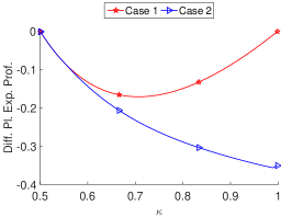
Figure 2.

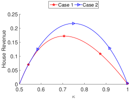
Figure 3.

Example 5.3.

Still, there are cases in which diffuse players are positively affected by the activities of the atomic player.

We now choose $\mu=\mu_{1}$ and $q=0.57$ for Cases 1 and 2. The actual probability of Outcome 1 is 0.47. The only difference between the two scenarios is that $w=10^{-10}$ in Case 1, while $w=1$ in Case 2.

Compared to Example 5.2, Outcome 1 is slightly less likely here. Also, we still assume that the atomic player’s forecast is quite accurate, but her prediction is no longer perfect.

We plot the diffuse players’ actual expected profit in Figure 5. The graphs for Cases 1 and 2 are the same for most values of $\kappa$; however, we see that the diffuse players’ expected profit is higher in Case 2 when $\kappa$ is large enough. Roughly, the atomic player does not start betting (on Outcome 1) until the house take is low, since she is nearly ambivalent. This explains why the curves are initially identical. When the atomic player begins to wager on Outcome 1, the diffuse players reshuffle their bets as in Example 5.2. The shift benefits them, essentially because the atomic player wagers on the wrong outcome.

In Figure 5, we plot the house’s revenue. We see an extremely small improvement in Case 2 when $\kappa$ is large, but the graphs are almost indistinguishable, visually. As in Example 5.2, the increase corresponds to the increase in the total amount wagered. It is slight, as the atomic player’s uncertainty about what will occur causes her to bet very little in Case 2, even for $\kappa\approx 1$.

Figure 4.

Figure 5.

Example 5.4.

We can argue that the diffuse players are better off in the presence of the atomic player, even without making assumptions about the actual probability of Outcome 1.

In Cases 1 and 2, we now choose $\mu=\mu_{10}$ and $q=0.95$. As in Examples 5.2 - 5.3, we set $w=10^{-10}$ in Case 1 and $w=1$ in Case 2. The atomic player believes that Outcome 1 is highly likely. Collectively, the diffuse players believe that Outcome 2 will probably happen: over $90\%$ of their initial wealth is held by those who believe that the probability of Outcome 2 is at least 0.9. We make no judgment about the accuracy of the players’ beliefs.

We plot the diffuse players’ subjective expected profit in Figure 7. The graphs are the same for low $\kappa$, but eventually, the diffuse players’ subjective expected profit is much higher in Case 2. Intuitively, the atomic player raises her wager on Outcome 1 as $\kappa\uparrow 1$, since she believes that Outcome 1 will occur. The implied probability of Outcome 1 then rises, a boon to those who believe that Outcome 2 will occur. This includes most of the diffuse players.

In Figure 7, we plot the house’s revenue. The house’s revenue in Case 2 is at least as large as its revenue in Case 1 for all values of $\kappa$. Often, the improvement is significant. Roughly, there is too much agreement among the diffuse bettors. They wager more in the presence of the atomic player, believing that they can profit from her supposed wagering mistakes. The pool size increases, leading to greater revenue for the house in Case 2.

Figure 6.

Figure 7.

Example 5.5.

In keeping with the standard narrative, it seems like the house is always immediately better off because of the atomic player. We can cast some doubt on this too.

We used the same $\mu$ for Cases 1 and 2 in Examples 5.2 - 5.4. This choice captures the idea that the presence of the atomic player should not affect the diffuse players’ initial wealth in a static parimutuel wagering game.

Alternatively, it might be reasonable to fix the distribution of initial wealth across the entire population, not just the diffuse population. For instance, we could specify that the amount held by those who believe that Outcome 1 will occur is roughly the same as the amount held by those who believe that Outcome 2 will occur. We could then compare the situations in which the wealth is held by only diffuse players and in which some wealth is held by the atomic player. This is the approach we now take.

In Case 1, $w=10^{-10}$ and the density of $\mu$ is defined by

$$p\mapsto\frac{g_{100}\left(p\right)+g_{100}\left(1-p\right)}{2}.$$

For Case 2, we set $w=1$ and $\mu=\mu_{100}$. We choose $q=1$ for both scenarios and, again, make no assumption about Outcome 1’s actual probability.

Intuitively, half of the diffuse players in Case 1 believe that Outcome 1 is going to occur, while the other half believes that Outcome 2 will occur. For Case 2, the diffuse players all believe that Outcome 2 is going to occur. The atomic player, whose wealth is equal to the collective wealth of the diffuse players, believes that Outcome 1 will occur.

Notice that the diffuse players’ total initial wealth is equal in Cases 1 and 2; however, the wealth of the entire population in Case 2 is twice what it is in Case 1. This is consistent with our parameter selections in Examples 5.2 - 5.4. When studying the house’s revenue here, we might have also chosen $\mu=0.5\times\mu_{100}$ and $w=0.5$ in Case 2, ensuring that the wealth of the entire population is identical in both scenarios. We comment on this shortly.

One might suspect that Cases 1 and 2 are quite similar, but this is not true. In Figure 9, we plot the diffuse players’ subjective expected profit. For $\kappa\approx 1$, their subjective expected profit is higher in Case 2 than in Case 1. Otherwise, it is lower for all $\kappa$, and often, the drop is significant.

To explain this observation, we plot the implied probability of Outcome 1 in Figure 9. The implied probability of Outcome 1 is about 0.5 for all $\kappa$ in Case 1. For Case 2, it is almost $1-\kappa$ for low $\kappa$ but approaches $0.5$ as $\kappa\uparrow 1$.

Since the diffuse players believe that Outcome 2 will occur but the atomic player believes that Outcome 1 will occur, the intuition appears to be as follows. Roughly, the diffuse players are willing to tolerate unfavorable betting conditions more than the atomic player. Despite the fact that each type of player is basically sure that the outcome they are betting on will occur, the diffuse players in Case 2 raise the size of their wagers much faster than the atomic player when $\kappa$ is low. The diffuse players do this at the expense of their own subjective expected profit, which is nearly zero in Case 2 until $\kappa\approx 0.84$. The atomic player does not substantially raise her wager on Outcome 1 until the values of the implied probability of Outcome 1 and $\kappa$ make her subjective expected profit per unit bet very high.

One could argue that the atomic player’s strategy is superior to the strategies employed by the diffuse players, although we have made no assumption about the accuracy of her prediction. Perhaps the reason is that unlike the diffuse players, she considers her individual impact on the other wagerers because of her substantial wealth.

In Figure 11, we plot the house’s revenue. We see that the house’s revenue is higher in Case 1 for small $\kappa$ but higher in Case 2 for large $\kappa$. After selecting $\mu=0.5\times\mu_{100}$ and $w=0.5$ in Case 2 (see our explanation above), we re-plot the house’s revenue in Figure 11. Now the house’s revenue is higher in Case 1 for all $\kappa$. Regardless of our normalization, the key point is that the house’s maximum revenue is always much higher in Case 1.

Intuitively, the diffuse players appear to have a greater tolerance for poor betting conditions than the atomic player, as discussed previously. They are willing to bet even when $\kappa\approx 0.5$, and consequently, about $99\%$ of the diffuse players are wagering in Case 1 when $\kappa\approx 0.51$. The house loses revenue by raising $\kappa$, since the entire population has already wagered almost everything that it can. In Case 2, the atomic player’s reluctance to significantly raise her wager on Outcome 1 until betting conditions improve means that the total amount wagered is low for most $\kappa$. The pool is large only if $\kappa$ is quite high, so the house does not collect much.

In Examples 5.2 - 5.4, the house’s revenue in Case 2 is at least as great as the house’s revenue in Case 1 for all $\kappa$. Of course, the house’s maximum revenue is then higher in Case 2 for these studies. Here, the pointwise analysis is not as clean, leading us to more directly consider the house’s strategic behavior.

Thus far, we have understood the house take to be exogenously determined. One way to relax this assumption is to break our game into two stages. In the first stage, the betting organizer chooses a value for the house take in order to maximize her revenue. The second stage is identical to our current setup.

Under the new framework, the house needs to account for more than the distribution of initial wealth across the entire population. The house must also consider how the initial wealth is distributed across the population for each type of player. Independent of our normalization of the entire population’s wealth, the house’s revenue is maximized at $\kappa\approx 0.506$ in Case 1 and at $\kappa\approx 0.839$ in Case 2. Hence, the house selects these values of $\kappa$ in Cases 1 and 2, respectively.

In Figure 9, the diffuse players’ subjective expected profit is about 0.0085 when $\kappa\approx 0.506$ in Case 2, while it is about 0.023 when $\kappa\approx 0.839$ in Case 2. These numbers arise from our original parameter choices, ensuring that the total initial wealth of the diffuse players is 1 in both scenarios. The diffuse players are not well off in either Case 1 or Case 2. We could still argue that the setup of Case 2 is to their advantage, in contrast to our earlier pointwise analysis. Roughly, because the atomic player is less willing to bet under poor wagering conditions, the house more easily preys upon the diffuse players when she is absent.

Figure 8.

Figure 9.

Figure 10.

Figure 11.

Appendix A Properties of $P^{f^{\star},a^{\star}}$

We briefly revisit our discussion of Corollary 4.6 by studying the properties of $P^{f^{\star},a^{\star}}$ as a function of $\kappa$. We hope this highlights a few theoretical features of our model, though we do not relate our findings in Appendix A to our central question. To generate these figures, we use the approach and notation of Section 5.

Recall our claim that in an extreme case where nearly all of the initial wealth is held by those who believe that Outcome 2 is highly likely, $P^{f^{\star},a^{\star}}\approx 1-\kappa$ for all $\kappa$. We illustrate this in Figure 13, which depicts the map $\kappa\mapsto P^{f^{\star},a^{\star}}$ when $\mu=\mu_{100}$, $q=0$, and $w=1$. Here, over 99% of the diffuse players’ initial wealth belongs to those who believe that the probability of Outcome 2 is at least 0.99. The atomic player believes that Outcome 2 is guaranteed to occur. As expected, the plot is visually indistinguishable from a plot of the map $\kappa\mapsto 1-\kappa$.

Often, it is more difficult to broadly describe attributes of the function $\kappa\mapsto P^{f^{\star},a^{\star}}$. We know that $P^{f^{\star},a^{\star}}\in\left(1-\kappa,\kappa\right)$, but our players’ heterogeneity allows for a wide range of possibilities within these bounds. There is a rich interplay between their differing beliefs, effects on (1.2), and wealth constraints. By plotting the map $\kappa\mapsto P^{f^{\star},a^{\star}}$ under varying assumptions on $q$, $w$, and $\mu$, Figure 13 displays a few of the myriad possibilities. For instance, the density $g$ of the $\mu$ used to generate Line $A$ is a linear combination of Gaussian densities with different means. Line $A$’s oscillations arise because of $g$’s distinct peaks.

Figure 12.

Figure 13.

Appendix B Proof of Proposition 4.2

We only prove (i). The argument for (ii) is similar, and as observed above, (iii) is due to Isaacs ([28]).

Suppose that (4.4) holds. Then

$$\frac{1-q}{d_{2}}<\displaystyle\frac{1-\kappa q}{d_{2}}<\displaystyle\frac{1}{d_{1}+d_{2}}<\displaystyle\frac{1}{\kappa\left(d_{1}+d_{2}\right)}<\displaystyle\frac{q}{d_{1}}.$$ (B.1)

We get the first and third inequalities because $\kappa\in\left(0,1\right)$. The second inequality is due to (4.9), while the last inequality is a rearrangement of (4.4). For now, the critical observation is that the leftmost quantity is less than the rightmost, allowing us to use the work of Isaacs ([28]).

Define the map

$$\Phi:\mathbb{R}^{2}_{\geq 0}\longrightarrow\mathbb{R}$$

by

$$\Phi\left(b_{1},b_{2}\right) =b_{1}\left(\displaystyle\frac{\kappa\left(b_{1}+d_{1}+b_{2}+d_{2}\right)q}{b_{1}+d_{1}}-1\right)+b_{2}\left(\displaystyle\frac{\kappa\left(b_{1}+d_{1}+b_{2}+d_{2}\right)\left(1-q\right)}{b_{2}+d_{2}}-1\right).$$

$\Phi\left(b_{1},b_{2}\right)$ is the atomic player’s expected profit, given that she wagers $b_{i}$ on Outcome $i$, and it allows us to rewrite (4.2) as

$$a_{1}\bigg{(}\displaystyle\frac{\kappa\,q}{P^{f,a}}-1\bigg{)}+a_{2}\left(\displaystyle\frac{\kappa\,\left(1-q\right)}{1-P^{f,a}}-1\right)=\displaystyle\sup_{\begin{subarray}{c}b_{1},b_{2}\geq 0\\ b_{1}+b_{2}\leq w\end{subarray}}\Phi\left(b_{1},b_{2}\right).$$

Technically, strategy profiles $\left(b_{1},b_{2}\right)$ with

$$b_{1}+b_{2}>w$$

are not feasible, but this is unimportant.

Isaacs showed that $\Phi$ has a unique global maximum on $\mathbb{R}^{2}_{\geq 0}$, denoted $\left(b_{1}^{\star},b_{2}^{\star}\right)$, given by

$$\left(b_{1}^{\star},b_{2}^{\star}\right)=\left(\displaystyle\sqrt{\displaystyle\frac{\kappa qd_{1}d_{2}}{1-\kappa q}}-d_{1},0\right).$$

This proves that (i) holds when $w\geq b_{1}^{\star}$.

The case where $w<b_{1}^{\star}$ is handled with elementary calculus. First, observe that (4.4) implies that $q>0$ and

$$\partial_{b_{1}}\Phi\left(0,0\right)=\displaystyle\frac{\kappa\left(d_{1}+d_{2}\right)q}{d_{1}}-1>0.$$

Since $\partial_{b_{1}}\Phi\left(b_{1}^{\star},0\right)=0$ and

$$\partial_{b_{1}b_{1}}\Phi\left(b_{1},b_{2}\right)=-\displaystyle\frac{2\kappa d_{1}\left(b_{2}+d_{2}\right)q}{\left(b_{1}+d_{1}\right)^{3}}$$

is always negative, it follows that $\partial_{b_{1}}\Phi\left(b_{1},0\right)>0$ for $0\leq b_{1}<b_{1}^{\star}$. The interpretation is that as long as the atomic player has not yet wagered on Outcome 2, she should wager as much as she can up to $b_{1}^{\star}$ on Outcome 1.

We only need to argue that she should never wager on Outcome 2, that is, $\partial_{b_{2}}\left(b_{1},b_{2}\right)$ is negative whenever $b_{1}+b_{2}\leq w$. Rearranging (B.1) implies that

$$\partial_{b_{2}}\Phi\left(0,0\right)=\displaystyle\frac{\kappa\left(d_{1}+d_{2}\right)\left(1-q\right)}{d_{2}}-1<0.$$

Now $\partial_{b_{2}}\Phi\left(b_{1}^{\star},0\right)\leq 0$ and

$$\partial_{b_{2}b_{1}}\Phi\left(b_{1},b_{2}\right)=\displaystyle\frac{\kappa d_{1}q}{\left(b_{1}+d_{1}\right)^{2}}+\displaystyle\frac{\kappa d_{2}\left(1-q\right)}{\left(b_{2}+d_{2}\right)^{2}}$$

is positive everywhere, so $\partial_{b_{2}}\Phi\left(b_{1},0\right)<0$ for $0\leq b_{1}<b_{1}^{\star}$. Since

$$\partial_{b_{2}b_{2}}\Phi\left(b_{1},b_{2}\right)=-\displaystyle\frac{2\kappa d_{2}\left(b_{1}+d_{1}\right)\left(1-q\right)}{\left(b_{2}+d_{2}\right)^{3}}$$

is always non-positive, we conclude that $\partial_{b_{2}}\left(b_{1},b_{2}\right)$ must be negative whenever $0\leq b_{1}<b_{1}^{\star}$. In particular, $\partial_{b_{2}}\left(b_{1},b_{2}\right)$ is negative, if $b_{1}+b_{2}\leq w$.

∎

Appendix C Proof of Theorem 4.3

Step 1: If $\left(f^{\star},a^{\star}\right)$ is an equilibrium, then $d_{1}^{\star}$, $d_{2}^{\star}>0$.

We show that the total amount wagered on each outcome by the diffuse players is positive in equilibrium: $d_{1}^{\star}$, $d_{2}^{\star}>0$. We use this result to complete the proof of the only if direction of Theorem 4.3 in Step C. It also allows us to use Propositions 4.1 and 4.2 in the proof of the if direction.

Suppose instead that we can find a pure-strategy Nash equilibrium $\left(f^{\star},a^{\star}\right)$ with $d_{1}^{\star}=0$. It follows immediately that $d_{2}^{\star}>0$: otherwise, (iii) of Definition 3.3 implies that $a_{1}^{\star}=a_{2}^{\star}=0$, which contradicts (i) of Definition 3.3. A consequence of Isaacs’ work is that $q=0$ ([28]). Then (iii) of Definition 3.3 implies that $a_{1}^{\star}=a_{2}^{\star}=0$. In particular, $P^{f^{\star},a^{\star}}=0$. By (i) of Definition 3.3, $f_{2}^{\star}\equiv 0$, which is impossible since $d_{2}^{\star}>0$.

Hence, $d_{1}^{\star}>0$. It follows similarly that $d_{2}^{\star}>0$.

Step 2: If an equilibrium exists, then $\kappa>0.5$.

We finish the proof of the only if direction of Theorem 4.3 by formalizing the heuristics given previously. Suppose that $\left(f^{\star},a^{\star}\right)$ is an equilibrium. Step C implies that $d_{1}^{\star}$, $d_{2}^{\star}>0$. Then both

$$\frac{P^{f^{\star},a^{\star}}}{\kappa}<1\qquad\text{and}\qquad\displaystyle\frac{1-P^{f^{\star},a^{\star}}}{\kappa}<1$$ (C.1)

by Proposition 4.1. Rearranging (C.1) finishes the argument.

Step 3: Definition and discussion of $\bar{p}_{i}$ (when $\kappa>0.5$).

Due to Step C, we assume that $\kappa>0.5$ for the remainder of the proof (Steps C - C). This assumption ensures that our discussions are not vacuous, as we implicitly rely on the positive length of the interval $\left[1-\kappa,\kappa\right]$.

We now define and discuss the quantities $\bar{p}_{1}$, $\bar{p}_{2}\in\left[1-\kappa,\kappa\right]$. We use this notation when we define our $\zeta_{i}$ maps in Step C and $\varphi$ in Step C. Roughly, $\bar{p}_{1}$ is a naïve lower bound for the implied probability of Outcome 1 when the atomic player wagers on Outcome 1. Similarly, $\bar{p}_{2}$ is an upper bound for the implied probability of Outcome 1 when the atomic player wagers on Outcome 2. Both are derived from Propositions 4.1 and 4.2.

Since $\mu$’s density is positive, the map

$$p\mapsto\displaystyle\frac{\mu\left(\frac{p}{\kappa},1\right]}{\kappa\left(\mu\left(\frac{p}{\kappa},1\right]+\mu\left[0,1-\frac{1-p}{\kappa}\right)\right)}$$ (C.2)

is decreasing and continuous on $\left[1-\kappa,\kappa\right]$. Its value is $1/\kappa$ at $p=\left(1-\kappa\right)$ and 0 at $p=\kappa$. Hence, there is a unique $\bar{p}_{1}\in\left(1-\kappa,\kappa\right]$ such that

$$q=\displaystyle\frac{\mu\left(\frac{\bar{p}_{1}}{\kappa},1\right]}{\kappa\left(\mu\left(\frac{\bar{p}_{1}}{\kappa},1\right]+\mu\left[0,1-\frac{1-\bar{p}_{1}}{\kappa}\right)\right)}.$$ (C.3)

Clearly, $\bar{p}_{1}=\kappa$, or equivalently, $\left(\bar{p}_{1},\kappa\right]$ is empty, if and only if $q=0$. Regardless of $q$’s value, we know

$$\left\{\begin{array}[]{cc}q\leq\displaystyle\frac{\mu\left(\frac{p}{\kappa},1\right]}{\kappa\left(\mu\left(\frac{p}{\kappa},1\right]+\mu\left[0,1-\frac{1-p}{\kappa}\right)\right)}&\qquad\text{if}\quad p\in\left[1-\kappa,\bar{p}_{1}\right]\\ &\\ q>\displaystyle\frac{\mu\left(\frac{p}{\kappa},1\right]}{\kappa\left(\mu\left(\frac{p}{\kappa},1\right]+\mu\left[0,1-\frac{1-p}{\kappa}\right)\right)}&\qquad\text{if}\quad p\in\left(\bar{p}_{1},\kappa\right]\end{array}\right..$$ (C.7)

We later connect this observation to (4.4) and (4.8) when defining $\zeta_{i}$ and $\varphi$.

Similarly, the map

$$p\mapsto\displaystyle\frac{\mu\left[0,1-\frac{1-p}{\kappa}\right)}{\kappa\left(\mu\left(\frac{p}{\kappa},1\right]+\mu\left[0,1-\frac{1-p}{\kappa}\right)\right)}$$ (C.8)

is increasing and continuous on $\left[1-\kappa,\kappa\right]$. Its value is 0 at $p=\left(1-\kappa\right)$ and $1/\kappa$ at $p=\kappa$, so there is a unique $\bar{p}_{2}\in\left[1-\kappa,\kappa\right)$ such that

$$1-q=\displaystyle\frac{\mu\left[0,1-\frac{1-\bar{p}_{2}}{\kappa}\right)}{\kappa\left(\mu\left(\frac{\bar{p}_{2}}{\kappa},1\right]+\mu\left[0,1-\frac{1-\bar{p}_{2}}{\kappa}\right)\right)}.$$

Now $\bar{p}_{2}=\left(1-\kappa\right)$, i.e., $\left[1-\kappa,\bar{p}_{2}\right)$ is empty, if and only if $q=1$. In any case,

$$\left\{\begin{array}[]{cc}1-q>\displaystyle\frac{\mu\left[0,1-\frac{1-p}{\kappa}\right)}{\kappa\left(\mu\left(\frac{p}{\kappa},1\right]+\mu\left[0,1-\frac{1-p}{\kappa}\right)\right)}&\qquad\text{if}\quad p\in\left[1-\kappa,\bar{p}_{2}\right)\\ &\\ 1-q\leq\displaystyle\frac{\mu\left[0,1-\frac{1-p}{\kappa}\right)}{\kappa\left(\mu\left(\frac{p}{\kappa},1\right]+\mu\left[0,1-\frac{1-p}{\kappa}\right)\right)}&\qquad\text{if}\quad p\in\left[\bar{p}_{2},\kappa\right]\end{array}\right..$$ (C.12)

This comment relates to (4.6) and (4.8), as reflected in our definitions of $\zeta_{i}$ and $\varphi$.

We conclude by observing that we have $\bar{p}_{2}<\bar{p}_{1}$ since $\kappa\in\left(0.5,1\right)$. This is another key remark for our future definition of $\varphi$.

Step 4: Definition and discussion of $\zeta_{i}$ (when $\kappa>0.5$).

We define and discuss the functions $\zeta_{1}$ and $\zeta_{2}$. We use this notation in our definition of $\varphi$ in Step C. Intuitively, $\zeta_{i}\left(p\right)$ represents the amount that the atomic player wagers on Outcome $i$ when she makes a positive wager on Outcome $i$, does not face a budget constraint, and the implied probability of Outcome 1 is $p$ (cf. (4.5) and (4.7)).

For $p\in\left[\bar{p}_{1},\kappa\right]$, define $\zeta_{1}$ by

$$\zeta_{1}\left(p\right)=\sqrt{\frac{\kappa q}{1-\kappa q}\,\mu\left(\frac{p}{\kappa},1\right]\mu\left[0,1-\frac{1-p}{\kappa}\right)}-\mu\left(\frac{p}{\kappa},1\right].$$

Since $\mu$ has a positive density, (C.7) implies that

$$\mu\left(\frac{p}{\kappa},1\right]>0,\qquad\mu\left[0,1-\frac{1-p}{\kappa}\right)>0,\qquad\text{and}\qquad q>\displaystyle\frac{\mu\left(\frac{p}{\kappa},1\right]}{\kappa\left(\mu\left(\frac{p}{\kappa},1\right]+\mu\left[0,1-\frac{1-p}{\kappa}\right)\right)}$$

for $p\in\left(\bar{p}_{1},\kappa\right)$. It follows as in (4.9) that $\zeta_{1}$ is positive on $\left(\bar{p}_{1},\kappa\right)$. We also have

$$\zeta_{1}\left(\bar{p}_{1}\right)=\zeta_{1}\left(\kappa\right)=0$$

from (C.3).

We define $\zeta_{2}$ for $p\in\left[1-\kappa,\bar{p}_{2}\right]$ by

$$\zeta_{2}\left(p\right)=\sqrt{\frac{\kappa\left(1-q\right)}{1-\kappa\left(1-q\right)}\,\mu\left(\frac{p}{\kappa},1\right]\mu\left[0,1-\frac{1-p}{\kappa}\right)}-\mu\left[0,1-\frac{1-p}{\kappa}\right).$$

Using the techniques from our discussion of $\zeta_{1}$, we see that $\zeta_{2}$ is positive on $\left(1-\kappa,\bar{p}_{2}\right)$ and

$$\zeta_{2}\left(1-\kappa\right)=\zeta_{2}\left(\bar{p}_{2}\right)=0.$$

Step 5: Definition and discussion of $\varphi$ (when $\kappa>0.5$).

We introduce the implied probability map $\varphi$. We see in Steps C and C that a fixed-point of $\varphi$ corresponds to a pure-strategy Nash equilibrium in an obvious way and vice versa, which ultimately allows us to complete Theorem 4.3’s proof.

$\varphi$’s domain is the set of candidates $p$ for the implied probability of Outcome 1. We need only consider $p\in\left[1-\kappa,\kappa\right]$, as we observe in Step C. Proposition 4.1 says that

$$\mu\left(\frac{p}{\kappa},1\right]\qquad\text{and}\qquad\mu\left[0,1-\frac{1-p}{\kappa}\right)$$ (C.13)

are the total amounts wagered by the diffuse players on Outcomes 1 and 2, respectively. The atomic player’s wagers are described by Proposition 4.2. For example, if

$$q>\displaystyle\frac{\mu\left(\frac{p}{\kappa},1\right]}{\kappa\left(\mu\left(\frac{p}{\kappa},1\right]+\mu\left[0,1-\frac{1-p}{\kappa}\right)\right)},$$

that is, $p\in\left(\bar{p}_{1},\kappa\right]$, then the atomic player wagers nothing on Outcome 2 and

$$\min\left\{w,\zeta_{1}\left(p\right)\right\}$$

on Outcome 1. Recalculating the implied probability of Outcome 1 using these bets, we get

$$\frac{\displaystyle\min\left\{w,\zeta_{1}\left(p\right)\right\}+\mu\left(\frac{p}{\kappa},1\right]}{\displaystyle\min\left\{w,\zeta_{1}\left(p\right)\right\}+\mu\left(\frac{p}{\kappa},1\right]+\mu\left[0,1-\frac{1-p}{\kappa}\right)}$$

from Definition 3.2. We set $\varphi\left(p\right)$ to this value. In some sense, this procedure is only potentially meaningful when $p$ is equal to $\varphi\left(p\right)$, leading to our focus on fixed-points.

Here is the complete definition of $\varphi$ suggested by this explanation:

$$\varphi\left(p\right)=\left\{\begin{array}[]{cc}\displaystyle\frac{\mu\left(\frac{p}{\kappa},1\right]}{\displaystyle\min\left\{w,\zeta_{2}\left(p\right)\right\}+\mu\left(\frac{p}{\kappa},1\right]+\mu\left[0,1-\frac{1-p}{\kappa}\right)}&\quad\text{if}\quad p\in\left[1-\kappa,\bar{p}_{2}\right)\\ &\\ \displaystyle\frac{\mu\left(\frac{p}{\kappa},1\right]}{\mu\left(\frac{p}{\kappa},1\right]+\mu\left[0,1-\frac{1-p}{\kappa}\right)}&\quad\text{if}\quad p\in\left[\bar{p}_{2},\bar{p}_{1}\right]\\ &\\ \displaystyle\frac{\displaystyle\min\left\{w,\zeta_{1}\left(p\right)\right\}+\mu\left(\frac{p}{\kappa},1\right]}{\displaystyle\min\left\{w,\zeta_{1}\left(p\right)\right\}+\mu\left(\frac{p}{\kappa},1\right]+\mu\left[0,1-\frac{1-p}{\kappa}\right)}&\quad\text{if}\quad p\in\left(\bar{p}_{1},\kappa\right]\end{array}\right..$$

Observe that $\varphi$ is continuous on $\left[1-\kappa,\kappa\right]$ since $\mu$ has a positive density and $\zeta_{i}\left(\bar{p}_{i}\right)=0$ (see Step C). This helps us prove that $\varphi$ has a unique fixed-point in Step C.

Step 6: $\varphi$ is decreasing (when $\kappa>0.5$).

We show that $\varphi$ is decreasing. We use this property in Step C to argue that $\varphi$ has a unique fixed-point.

Since $\mu$’s density is positive everywhere, $\varphi$ is decreasing on $\left[\bar{p}_{2},\bar{p}_{1}\right]$. It suffices to show that $\varphi$ is decreasing on both $\left[1-\kappa,\bar{p}_{2}\right)$ and $\left(\bar{p}_{1},\kappa\right]$ because $\varphi$ is continuous. The proofs are similar, so we consider the former case.

We are done, if $\left[1-\kappa,\bar{p}_{2}\right)$ is empty. Suppose that it is not. Recall from Step C that this is equivalent to assuming that $q<1$. Define two functions $\varphi_{2}$ and $\varphi_{2}^{w}$ on $\left[1-\kappa,\bar{p}_{2}\right)$ by

$$\varphi_{2}\left(p\right) =\displaystyle\frac{\mu\left(\frac{p}{\kappa},1\right]}{\zeta_{2}\left(p\right)+\mu\left(\frac{p}{\kappa},1\right]+\mu\left[0,1-\frac{1-p}{\kappa}\right)}$$

$$\varphi_{2}^{w}\left(p\right) =\displaystyle\frac{\mu\left(\frac{p}{\kappa},1\right]}{w+\mu\left(\frac{p}{\kappa},1\right]+\mu\left[0,1-\frac{1-p}{\kappa}\right)}.$$

The point is that

$$\varphi\left(p\right)=\displaystyle\max\left\{\varphi_{2}\left(p\right),\varphi_{2}^{w}\left(p\right)\right\}$$

on $\left[1-\kappa,\bar{p}_{2}\right)$, so it is enough to show that $\varphi_{2}$ and $\varphi_{2}^{w}$ are both decreasing.

Clearly, $\varphi_{2}^{w}$ is decreasing. Denoting the positive and continuous density of $\mu$ by $g$, we see that $\varphi_{2}$ is decreasing because

$$\varphi_{2}^{\prime}\left(p\right) =-\displaystyle\frac{g\left(\frac{p}{\kappa}\right)\sqrt{\frac{\kappa\left(1-q\right)}{1-\kappa\left(1-q\right)}\mu\left(\frac{p}{\kappa},1\right]\mu\left[0,1-\frac{1-p}{\kappa}\right)}}{2\kappa\left(\sqrt{\frac{\kappa\left(1-q\right)}{1-\kappa\left(1-q\right)}\mu\left(\frac{p}{\kappa},1\right]\mu\left[0,1-\frac{1-p}{\kappa}\right)}+\mu\left(\frac{p}{\kappa},1\right]\right)^{2}}$$

$$\qquad-\displaystyle\frac{\left(\frac{\kappa\left(1-q\right)}{1-\kappa\left(1-q\right)}\right)^{0.5}\mu\left(\frac{p}{\kappa},1\right]^{3/2}\mu\left[0,1-\frac{1-p}{\kappa}\right)^{-0.5}g\left(1-\frac{1-p}{\kappa}\right)}{2\kappa\left(\sqrt{\frac{\kappa\left(1-q\right)}{1-\kappa\left(1-q\right)}\mu\left(\frac{p}{\kappa},1\right]\mu\left[0,1-\frac{1-p}{\kappa}\right)}+\mu\left(\frac{p}{\kappa},1\right]\right)^{2}}.$$

Step 7: $\varphi$ has a unique fixed-point (when $\kappa>0.5$).

We show that $\varphi$ has a unique fixed-point. We use the existence of $\varphi$’s fixed-point to prove the existence of a pure-strategy Nash equilibrium in Step C, while we use the uniqueness of $\varphi$’s fixed-point to demonstrate that the equilibrium is unique in Step C.

The proof is simple: $\varphi\left(1-\kappa\right)=1$ and $\varphi\left(\kappa\right)=0$. Since $\varphi$ is continuous and decreasing (see Steps C - C), it must have a unique fixed-point.

Step 8: An equilibrium exists (when $\kappa>0.5$).

We show that a pure-strategy Nash equilibrium exists. Based on Step C, we need only describe how to construct an equilibrium from a fixed-point of $\varphi$.

Suppose that $\hat{P}$ is a fixed-point of $\varphi$. The proofs for each case are similar, so we only present the argument when $\hat{P}\in\left[1-\kappa,\bar{p}_{2}\right)$. Define a feasible strategy profile $\left(f,a\right)$ by

$$f_{1}\left(p\right) =\left\{\begin{array}[]{cc}1&\quad\text{if }\,\,p\geq\hat{P}/\kappa\\ &\\ 0&\quad\text{if }\,\,p<\hat{P}/\kappa\\ \end{array}\right.,\qquad\qquad f_{2}\left(p\right)=\left\{\begin{array}[]{cc}1&\quad\text{if }\,\,1-p\geq\left(1-\hat{P}\right)/\kappa\\ &\\ 0&\quad\text{if }\,\,1-p<\left(1-\hat{P}\right)/\kappa\\ \end{array}\right.,$$

$a_{1}=0$, and

$$a_{2}=\displaystyle\min\left\{w,\zeta_{2}\left(\hat{P}\right)\right\}.$$

In particular,

$$d_{1}=\mu\left(\frac{\hat{P}}{\kappa},1\right]\qquad\text{and}\qquad d_{2}=\mu\left[0,1-\frac{1-\hat{P}}{\kappa}\right).$$

(C.12) implies that (4.6) is satisfied. Since $\varphi\left(1-\kappa\right)=1$, we know that $\hat{P}\neq\left(1-\kappa\right)$. Hence, $d_{1}$, $d_{2}>0$ because the density of $\mu$ is positive everywhere. We then have (iii) of Definition 3.3 by Proposition 4.2.

Since $\hat{P}$ is a fixed-point of $\varphi$,

$$\hat{P}=\frac{\mu\left(\frac{\hat{P}}{\kappa},1\right]}{\displaystyle\min\left\{w,\zeta_{2}\left(\hat{P}\right)\right\}+\mu\left(\frac{\hat{P}}{\kappa},1\right]+\mu\left[0,1-\frac{1-\hat{P}}{\kappa}\right)}=P^{f,a}.$$

From Proposition 4.1, we see that (ii) of Definition 3.3 holds.

This completes the proof, as (i) of Definition 3.3 is obviously satisfied.

Step 9: The equilibrium in Step C is unique (when $\kappa>0.5$).

We conclude Theorem 4.3’s proof by showing that the equilibrium in Step C is unique. The key observation is that $\varphi$’s fixed-point is also unique (see Step C).

First, we describe how to construct a fixed-point of $\varphi$, given an equilibrium $\left(f^{\star},a^{\star}\right)$. From Proposition 4.1 and Step C, we know that

$$d_{1}^{\star}=\mu\left(\frac{P^{f^{\star},a^{\star}}}{\kappa},1\right]>0\qquad\text{and}\qquad d_{2}^{\star}=\mu\left[0,1-\frac{1-P^{f^{\star},a^{\star}}}{\kappa}\right)>0.$$

In particular, $P^{f^{\star},a^{\star}}\in\left(1-\kappa,\kappa\right)$. By Proposition 4.2, there are three possibilities for $a^{\star}$.

Assume that $a_{1}^{\star}>0$ and $a_{2}^{\star}=0$. The other cases can be handled similarly. By Proposition 4.2, (4.4) holds. Hence, $P^{f^{\star},a^{\star}}\in\left(\bar{p}_{1},\kappa\right)$ due to (C.7) and

$$a_{1}^{\star}=\displaystyle\min\left\{w,\sqrt{\displaystyle\frac{\kappa qd_{1}^{\star}d_{2}^{\star}}{1-\kappa q}}-d_{1}^{\star}\right\}=\displaystyle\min\left\{w,\zeta_{1}\left(P^{f^{\star},a^{\star}}\right)\right\}.$$

By Definition 3.2,

$$P^{f^{\star},a^{\star}} =\displaystyle\frac{\displaystyle\min\left\{w,\zeta_{1}\left(P^{f^{\star},a^{\star}}\right)\right\}+\mu\left(\frac{P^{f^{\star},a^{\star}}}{\kappa},1\right]}{\displaystyle\min\left\{w,\zeta_{1}\left(P^{f^{\star},a^{\star}}\right)\right\}+\mu\left(\frac{P^{f^{\star},a^{\star}}}{\kappa},1\right]+\mu\left[0,1-\frac{1-P^{f^{\star},a^{\star}}}{\kappa}\right)}$$

$$=\varphi\left(P^{f^{\star},a^{\star}}\right),$$

that is, $P^{f^{\star},a^{\star}}$ is a fixed-point of $\varphi$.

Now suppose that we have another equilibrium $\left(f^{\diamond},a^{\diamond}\right)$. Using the method just described, we see that $P^{f^{\diamond},a^{\diamond}}$ is a fixed-point of $\varphi$. Since there is exactly one fixed-point of $\varphi$ by Step C, $P^{f^{\diamond},a^{\diamond}}=P^{f^{\star},a^{\star}}$.

By Step C and Proposition 4.1, $f^{\star}$ and $f^{\diamond}$ necessarily agree everywhere, except when

$$p=P^{f^{\star},a^{\star}}/\kappa\qquad\text{or}\qquad 1-p=\left(1-P^{f^{\star},a^{\star}}\right)/\kappa.$$

Since $\mu$ has a density, it follows that $f^{\star}=f^{\diamond}$ $\mu$-a.s. Clearly, $d_{1}^{\star}=d_{1}^{\diamond}$ and $d_{2}^{\star}=d_{2}^{\diamond}$. Proposition 4.2 implies that $a^{\star}=a^{\diamond}$.

∎

References

- [1] Euromillions information: pari-mutuel, Available at https://www.euro-millions.com/pari-mutuel. Accessed: 2016-03-01.
- [2] International Federation of Horseracing Authorities 2014 annual report. Available at http://www.horseracingintfed.com/default.asp?section=Resources&area=4&FF=15&statsyear=2014&report=D. Accessed: 2016-03-01.
- [3] P. Asch, B. G. Malkiel, and R. E. Quandt, Racetrack betting and informed behavior, Journal of Financial Economics, 10 (1982), pp. 187 – 194.
- [4] R. J. Aumann, Markets with a continuum of traders, Econometrica, 32 (1964), pp. 39–50.
- [5] E. J. Balder, On the existence of Cournot-Nash equilibria in continuum games, Journal of Mathematical Economics, 32 (1999), pp. 207 – 223.
- [6] , A unifying pair of Cournot-Nash equilibrium existence results, Journal of Economic Theory, 102 (2002), pp. 437 – 470.
- [7] K. Baron and J. Lange, Parimutuel applications in finance, Palgrave Macmillan UK, 2007.
- [8] R. N. Bolton and R. G. Chapman, Searching for positive returns at the track: a multinomial logit model for handicapping horse races, Management Science, 32 (1986), pp. 1040–1060.
- [9] É. Borel, Sur le pari mutuel, Comptes Rendus Hebdomadaires des Séances de l’Académie des Sciences, 207 (1938), pp. 197–200.
- [10] F. Canyameres, L’Homme de la Belle Époque, les Éditions universelles, Paris, 1946.
- [11] G. Carmona and K. Podczeck, Existence of Nash equilibrium in games with a measure space of players and discontinuous payoff functions, Journal of Economic Theory, 152 (2014), pp. 130 – 178.
- [12] R. Carmona and D. Lacker, A probabilistic weak formulation of mean field games and applications, Ann. Appl. Probab., 25 (2015), pp. 1189–1231.
- [13] S. Chadha and R. E. Quandt, Betting bias and market equilibrium in racetrack betting, Applied Financial Economics, 6 (1996), pp. 287–292.
- [14] P. Chan and R. Sircar, Bertrand and Cournot mean field games, Appl. Math. Optim., 71 (2015), pp. 533–569.
- [15] , Fracking, renewables & mean field games, SIAM Rev., (Forthcoming).
- [16] R. Cheung, Pari-mutuel wagering. Undergraduate Thesis, Princeton University, 1985.
- [17] S. Correa and J. P. Torres-Martínez, Essential equilibria of large generalized games, Economic Theory, 57 (2014), pp. 479–513.
- [18] R. Feeney and S. P. King, Sequential parimutuel games, Economics Letters, 72 (2001), pp. 165 – 173.
- [19] R. Gayduk and S. Nadtochiy, Endogenous formation of limit order books: the effects of trading frequency, ArXiv e-prints, (2015).
- [20] D. A. Gomes and V. K. Voskanyan, Extended deterministic mean-field games, ArXiv e-prints, (2013).
- [21] D. B. Hausch, V. S. Lo, and W. T. Ziemba, eds., Efficiency of Racetrack Betting Markets, World Scientific, Singapore, 2008 ed.
- [22] D. B. Hausch and W. T. Ziemba, eds., Handbook of sports and lottery markets, Handbooks in Finance, Elsevier, San Diego, 2008.
- [23] D. B. Hausch, W. T. Ziemba, and M. Rubinstein, Efficiency of the market for racetrack betting, Management Science, 27 (1981), pp. 1435–1452.
- [24] S. Herrmann, J. Muhle-Karbe, and F. T. Seifried, Hedging with small uncertainty aversion, Finance and Stochastics, 21 (2017), pp. 1–64.
- [25] M. Huang, Large-population LQG games involving a major player: the Nash certainty equivalence principle, SIAM Journal on Control and Optimization, 48 (2010), pp. 3318–3353.
- [26] M. Huang, R. P. Malhamé, and P. E. Caines, Large population stochastic dynamic games: closed-loop Mckean-Vlasov systems and the Nash certainty equivalence principle, Communications in Information & Systems, 6 (2006), pp. 221–252.
- [27] W. Hurley and L. McDonough, A note on the Hayek hypothesis and the favorite-longshot bias in parimutuel betting, The American Economic Review, (1995), pp. 949–955.
- [28] R. Isaacs, Optimal horse race bets, The American Mathematical Monthly, 60 (1953), pp. 310–315.
- [29] S. Jaimungal and M. Nourian, Mean-field game strategies for a major-minor agent optimal execution problem, Available at SSRN 2578733, (2015).
- [30] M. Kaplan, The high tech trifecta, Available at http://www.wired.com/2002/03/betting/.
- [31] F. Koessler, C. Noussair, and A. Ziegelmeyer, Parimutuel betting under asymmetric information, Journal of Mathematical Economics, 44 (2008), pp. 733 – 744. Special Issue in Economic Theory in honor of Charalambos D. Aliprantis.
- [32] F. Koessler, A. Ziegelmeyer, and M.-H. Broihanne, The favorite-longshot bias in sequential parimutuel betting with non-expected utility players, Theory and Decision, 54 (2003), pp. 231–248.
- [33] J. Lange and N. Economides, A parimutuel market microstructure for contingent claims, European Financial Management, 11 (2005), pp. 25–49.
- [34] J.-M. Lasry and P.-L. Lions, Mean field games, Japanese Journal of Mathematics, 2 (2007), pp. 229–260.
- [35] A. Mas-Colell, On a theorem of Schmeidler, Journal of Mathematical Economics, 13 (1984), pp. 201 – 206.
- [36] S. L. Nguyen and M. Huang, Linear-Quadratic-Gaussian mixed games with continuum-parametrized minor players, SIAM Journal on Control and Optimization, 50 (2012), pp. 2907–2937.
- [37] M. Nourian and P. E. Caines, -Nash mean field game theory for nonlinear stochastic dynamical systems with major and minor agents, SIAM Journal on Control and Optimization, 51 (2013), pp. 3302–3331.
- [38] M. Ottaviani and P. N. Sørensen, The timing of parimutuel bets, Available at http://faculty.london.edu/mottaviani/tobaflb.pdf, (2006).
- [39] M. Ottaviani and P. N. Sørensen, The favorite-longshot bias: an overview of the main explanations, in In Handbook of Sports and Lottery Markets, Elsevier North Holland, 2008.
- [40] M. Ottaviani and P. N. Sørensen, Surprised by the parimutuel odds?, The American Economic Review, 99 (2009-12-01T00:00:00), pp. 2129–2134.
- [41] D. M. Pennock, A dynamic pari-mutuel market for hedging, wagering, and information aggregation, in Proceedings of the 5th ACM Conference on Electronic Commerce, EC ’04, New York, NY, USA, 2004, ACM, pp. 170–179.
- [42] M. Peters, A. M.-C. So, and Y. Ye, Internet and Network Economics: Third International Workshop, WINE 2007, San Diego, CA, USA, December 12-14, 2007. Proceedings, Springer Berlin Heidelberg, Berlin, Heidelberg, 2007, ch. Pari-Mutuel Markets: Mechanisms and Performance, pp. 82–95.
- [43] R. C. Plott, J. Wit, and C. W. Yang, Parimutuel betting markets as information aggregation devices: experimental results, Economic Theory, 22, pp. 311–351.
- [44] J. Potters and J. Wit, Bets and bids: favorite-longshot bias and winner’s curse, CentER Discussion Paper, 1996-04.
- [45] R. E. Quandt, Betting and equilibrium, The Quarterly Journal of Economics, 101 (1986), pp. 201–207.
- [46] A. R. Villegas and J. P. Torres-Martínez, On pure strategy equilibria in large generalized games, Available at https://mpra.ub.uni-muenchen.de/46840/, year=2013.
- [47] K. P. Rath, A direct proof of the existence of pure strategy equilibria in games with a continuum of players, Economic Theory, 2 (1992), pp. 427–433.
- [48] B. Rosner, Optimal allocation of resources in a pari-mutuel setting, Management Science, 21 (1975), pp. 997–1006.
- [49] D. Schmeidler, Equilibrium points of nonatomic games, Journal of Statistical Physics, 7 (1973), pp. 295–300.
- [50] D. Terrell and A. Farmer, Optimal betting and efficiency in parimutuel betting markets with information costs, The Economic Journal, 106 (1996), pp. 846–868.
- [51] R. H. Thaler and W. T. Ziemba, Parimutuel betting markets: racetracks and lotteries, Journal of Economic Perspectives, 2 (1988), pp. 161–74.
- [52] R. M. Thrall, Some results in non-linear programming, in Proceedings of the Second Symposium in Linear Programming, Washington, D. C., 1955, National Bureau of Standards, Washington, D. C., 1955, pp. 471–493.
- [53] Y. Wang, F. Yu, H. Tang, and M. Huang, A mean field game theoretic approach for security enhancements in mobile ad hoc networks, Wireless Communications, IEEE Transactions on, 13 (2014), pp. 1616–1627.
- [54] T. Watanabe, A parimutuel system with two horses and a continuum of bettors, Journal of Mathematical Economics, 28 (1997), pp. 85 – 100.
- [55] T. Watanabe, H. Nonoyama, and M. Mori, A model of a general parimutuel system: characterizations and equilibrium selection, International Journal of Game Theory, 23, pp. 237–260.
- [56] R. J. Weber, Noncooperative games, in Game theory and its applications (Biloxi, Miss., 1979), vol. 24 of Proc. Sympos. Appl. Math., Amer. Math. Soc., Providence, R.I., 1981, pp. 83–125.
- [57] A. Wiszniewska-Matyszkiel, Dynamic oligopoly as a mixed large game–toy market, in Mathematical programming and game theory for decision making, vol. 1, World Scientific, Singapore, 2008, pp. 369–390.