Monte Carlo radiation transfer simulations of photospheric emission in long-duration Gamma-Ray Bursts

Abstract

We present MCRaT, a Monte Carlo Radiation Transfer code for self-consistently computing the light curves and spectra of the photospheric emission from relativistic, unmagnetized jets. We apply MCRaT to a relativistic hydrodynamic simulation of a long duration gamma-ray burst jet, and present the resulting light-curves and time-dependent spectra for observers at various angles from the jet axis. We compare our results to observational results and find that photospheric emission is a viable model to explain the prompt phase of long-duration gamma-ray bursts at the peak frequency and above, but faces challenges in reproducing the flat spectrum below the peak frequency. We finally discuss possible limitations of these results both in terms of the hydrodynamics and the radiation transfer and how these limitations could affect the conclusions that we present.

1. Introduction

Photospheric emission is a leading model to explain the prompt radiation of long-duration gamma-ray bursts (Rees & Mészáros, 2005; Giannios, 2006; Lazzati et al., 2009; Lundman et al., 2013; Peer, 2015). In the photospheric model the radiation is assumed to form deep in the outflow, where the jet is highly optically thick, and to be advected out, eventually being released when the jet becomes transparent. The photospheric model does not specify the radiation mechanism involved, since the spectrum is shaped by the interaction with matter, mostly through Compton scattering, and not by the emission process itself.

The alternative model, the Synchrotron Shock Model (SSM, Rees & Meszaros 1994; Daigne & Mochkovitch 1998; Lloyd-Ronning & Petrosian 2002; Daigne et al. 2011; Zhang & Yan 2011), assumes instead that the jet crosses the photosphere virtually deprived of radiation, coasts until the Thomson optical depth is well below unity, and is reactivated when shells of different speed shock each other and generate non-thermal particles and magnetic field (Rees & Meszaros, 1994). SSM predicts that the radiation spectrum is directly related to the radiation mechanism and suffers little interaction with the baryons and leptons of the jet once it is produced. Both models have been successful in explaining some of the observed properties of long duration GRBs but are in significant tension with other properties. For example, SSM easily accounts for the non-thermal, broadband nature of the prompt spectrum (Piran, 1999), but faces challenges for its intrinsic width (Vurm & Beloborodov, 2015) and when compared to ensemble correlations such as the Amati, Yonetoku, Golenetskii, or E-$\Gamma$ correlations (Golenetskii et al., 1983; Amati et al., 2002; Yonetoku et al., 2004; Liang et al., 2010; Ghirlanda et al., 2012). On the other hand, the photospheric emission has been shown to be able to reproduce all the correlations (Lazzati et al. 2011, 2013, hereafter L13; López-Cámara et al. 2014) but can hardly produce a spectrum that has prominent non-thermal tails at both low- and high-frequencies. While sub-photospheric dissipation can cure the high-frequency problem producing prominent non-thermal tails (Pe’er et al., 2006; Giannios, 2006; Giannios & Spruit, 2007; Beloborodov, 2010; Lazzati & Begelman, 2010; Vurm et al., 2011; Ito et al., 2013, 2014; Chhotray & Lazzati, 2015; Santana et al., 2016), it is still unclear whether the low-frequency tails can be reproduced in photon-starved conditions without invoking an external radiation mechanism such as synchrotron (Pe’er & Ryde, 2011; Chhotray & Lazzati, 2015). Encouraging results, however, have been obtained for photospheric emission with contributions from an subdominant synchrotron component (Vurm & Beloborodov, 2015).

In both cases, theoretical models only partially address the complexity of the GRB phenomenon. With very few exceptions, models either simplify the radiation physics or the geometry of the emitting region. For example, photospheric radiation computed from jet simulations – and therefore fully taking into account the complexity of structured and turbulent outflows – assume that the radiation-matter coupling is infinite below the photosphere but suddenly drops to zero as soon as the photosphere is crossed (e.g., Lazzati et al. 2009; Mizuta et al. 2011; Nagakura et al. 2011; L13). On the other hand, models that consider proper radiation transfer or radiation from magnetized jets with dissipation and particle acceleration are applied to simplified homogeneous plasma regions or to spherical jets with analytic radial stratification and without any polar structure (e.g., Pe’er et al. 2006; Giannios & Spruit 2007; Beloborodov 2010; Lazzati & Begelman 2010; Vurm et al. 2011; Chhotray & Lazzati 2015; Vurm & Beloborodov 2015; Beloborodov 2016).

In this paper we present the results of a first step towards merging the two worlds and performing detailed radiation transfer calculations on the complex dynamics of a relativistic jet from high-resolution multi-dimensional numerical simulations (analogous to the recent work by Ito et al. 2015). In Section 2 we present the Monte Carlo Radiation Transfer (MCRaT) code and the results of several validation tests. In Section 3 we present and discuss the results of applying the code to a hydrodynamic (HD) simulation of a GRB jet. Finally, in Section 4 we discuss our results by comparing them with observations and previous theoretical work, and we discuss limitations and possible improvements of this technique.

2. The MCRaT code

We developed a Monte Carlo Radiation Transfer (MCRaT code) to compute time-resolved light curves and spectra from hydrodynamic simulations of GRB jets. The approach to the single-photon scattering in the code is to neglect the energy losses of the electron population, randomly selecting at each scattering an electron from a thermal population at a temperature that does not depend on previous scatterings. This is a fairly standard approach that assumes the heat capacity of the fluid to be large enough that radiation losses can be neglected (e.g. Giannios 2006; Ito et al. 2013). The novelty of the code is that of performing the radiation transfer on the fast evolving background of a relativistic outflow (Ito et al., 2015). The code injects photons in thermal equilibrium with the fluid well inside the photosphere and performs repeated Compton and inverse Compton (IC) scattering off electrons that are at the local comoving temperature of the fluid. The present version of MCRaT takes two-dimensional simulations as input, but the photon propagation is done in three dimensions to properly take into account the photon propagation angle with respect to the fluid. In other words the photon field includes photons propagating in directions with non-zero azimuthal angle $\phi$, even if the fluid velocity is constrained to be only in the radial and polar direction. In more detail, the code performs the following steps (see also Figure 1):

• Photon injection – Photons are injected at a user specified radius $R_{\mathrm{inj}}$ and within a user specified range of polar angles from the jet axis. The code determines the local temperature, density, and velocity vector at the photon’s position by nearest-neighbor interpolation. This can be switched to linear interpolation at the cost of a longer computational time, but with no visible effect on the results. The photon 4-momentum ${\mathbf{p}_{\gamma}}$ is generated by randomly sampling a thermal photon distribution at the local fluid temperature. The distribution can be chosen between a black body and a Wien spectrum, the former being appropriate for fireballs in the acceleration stage, the latter for fireballs in the coasting phase. The photons’ direction of propagation is assumed to be isotropic in the fluid’s rest frame at injection. Since it is clearly impossible to simulate all the photons in a GRB fireball (their number amounting to $\sim 10^{59}$ for a typical burst), each photon is assigned a weight:

  $$w_{\gamma,i}=\frac{8\pi\,c}{3N_{\rm{inj}}}\xi\,T^{\prime 3}_{i}\,\Gamma_{i}\,R_{i}^{2}\,\delta t\,\delta\theta\,\sin(\theta_{i})$$ (1)

  where $\xi$ is the coefficient for the photon number density ($n_{\gamma}$) in the equation $n_{\gamma}=\xi T^{3}$; $\xi=20.29$ for a black body and $\xi=8.44$ for a Wien spectrum; $T^{\prime}$ is the (comoving) fluid temperature at the photon location; $\Gamma_{i}$ is the fluid’s bulk Lorentz factor at the photon location; $R$ is the injection radius (in the Lab frame); $\delta t$ is the time resolution of the numerical simulation (time interval between two saved frames); $\delta\theta$ is the polar angular range in which the photons are injected (in the Lab frame); $\theta_{i}$ is the specific angle at which the $i$-th photon is injected (in the Lab frame); and $N_{\rm{inj}}$ is the number of photons injected in each frame of the simulation. The subscript $i$ is used for all quantities that are computed independently individually for each photon. The weights are chosen so that the sum of the energies of the injected photons times their weight gives the correct jet luminosity (see the Appendix for a derivation of the photons weight).

• Photon mean free path – The first step in the photons propagation is the calculation of their mean free path in the expanding fluid. This is computed as (Abramowicz et al., 1991):

  $$\lambda_{i}=\frac{dr}{d\tau_{T}}=\frac{1}{\sigma_{T}\,n_{i}^{\prime}\,\Gamma_{i}\,\left(1-\beta_{i}\cos\theta_{\mathrm{fl},i}\right)}$$ (2)

  where $\sigma_{T}$ is the Thomson cross-section, $n_{i}^{\prime}$ is the comoving lepton number density of the fluid at each photon position, $\beta_{i}$ is the fluid’s velocity at the photon position in units of the speed of light $c$, and $\theta_{\mathrm{fl},i}$ is the angle between the fluid and photon’s velocities. Note that the mean free path should in principle be integrated over the evolving fluid density and velocity. However, photons very rarely move out of their original hydrodynamic resolution element within the time span $\delta t$ between a scattering and the subsequent one, and therefore our approximation that the underlying hydrodynamic does not change between the times at which the mean free path is calculated is accurate. We also notice that we are assuming that the photon energies are well below the electron’s rest mass energy (511 keV) and we can ignore Klein-Nishina effects. In most cases, this is a good approximation for a GRB jet in the comoving frame.

• Selection of the interacting photon – Once all the mean free paths have been calculated, a random scattering time for each photon is drawn from the distributions:

  $$p_{i}(t)=\frac{c}{\lambda_{i}}\,e^{-\frac{c}{\lambda_{i}}t}$$ (3)

  The shortest of the obtained times is used as the next scattering time.

  

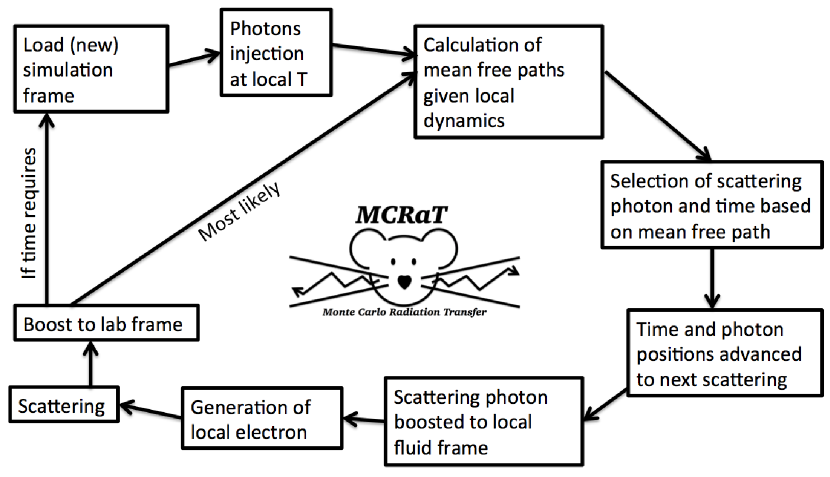
  Figure 1.— Block diagram of the main loop of the MCRaT code.

• Update of photon positions – At this point the code checks whether the selected collision time is within the time range of the current HD simulation frame. If so, all photons positions three-vectors $\mathbf{R_{i}}$ are updated by propagating the photons at the speed of light for the selected time interval. If not, a new time interval equal to the time remaining for the current HD simulation frame is selected, and all photons positions are updated. No scattering takes place in this case, a new HD frame is loaded, and the code returns to the mean free path step, computing a new mean free path for the photons in the updated HD and then selecting a new scattering time. Note that, when a new simulation frame is loaded, a new batch of photons is added at the injection radius following the rules of photon injection as described above in bullet “photon injection”.

  

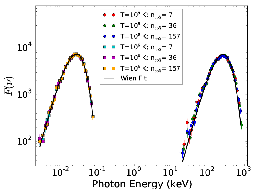
  Figure 2.— Spectra from a test simulation with a cylindrical outflow of constant velocity and temperature. Two simulations are shown, each at three different stages, for increasing number of scatterings per photon.

• Photon scattering – When the time and location of a photon scattering is identified, the code performs several steps. First, the photon four momentum $\mathbf{P_{i}}$ is transformed to the local fluid comoving frame. Second, an electron is randomly drawn from a Maxwell-Boltzmann or Maxwell-Jüttner distribution at the local fluid temperature $T_{i}$. The electron is assigned a direction of motion with a probability distribution $p(\psi)\propto\sin\psi(1-\beta\cos\psi)$, where $\psi$ is the angle between the photon and electron velocity vectors. Third, the electron and photon four momenta are transformed to the electron’s comoving frame, and the reference frame rotated so that the photon’s propagation is along the z-axis. A scattering angle is generated according to the Thomson probability distribution $p(\theta_{\mathrm{scatt}})\propto\sin\theta_{\mathrm{scatt}}(1+\cos^{2}\theta_{\mathrm{scatt}})$ and the post-scattering four momenta are computed according to momentum and energy conservation. Finally, the photon’s four momentum is rotated and doubly boosted back to the lab frame.

The loop described above is performed iteratively until the photons reach the edge of the simulation, or the last simulation frame is reached (see also Figure 1). Each time a new simulation frame is loaded, the code saves the photon position vectors and momenta four-vectors. In post processing, a script is used to generate a photon event table that contains the photons detected by a virtual detector placed at a certain distance from the burst and along a selected orientation. The event table contains photon detection time and energy and the photon weight $w_{\gamma,i}$.

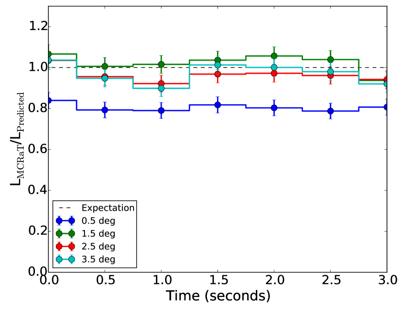
Figure 3.— Comparison between the expected luminosity and the one computed with MCRaT for a spherical relativistic outflow. For the line of sight very close to the singular polar axis we find a $\sim 20$ per cent deviation between the expected and obtained results. All the other lines of sight are fully consistent with the predicted luminosity.

2.1. Code Validation

In order to validate the MCRaT code we ran a suite of tests for which the expected result is known. All tests were run by imposing an analytic outflow solution on the same simulation frames that will be used in Section 3 to study the light curves and spectra of a long GRB simulation. This means that the grid setup (cell centers and sizes) was read from the simulation files, but the values of density, pressure, and velocity were substituted with an analytical solution as a function of the cell position. This way, the same spatial resolution of the tests is used for the scientific simulation and we can evaluate the influence of the grid size and resolution on the accuracy of the results.

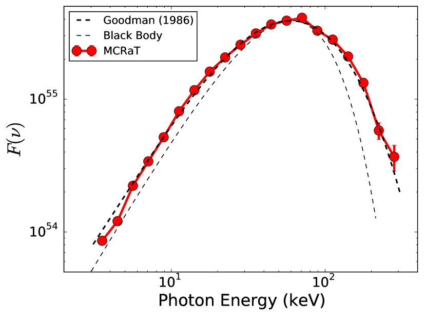
Figure 4.— MCRaT spectrum from a spherical outflow compared with a black body spectrum at the same temperature and with the prediction of Goodman (1986) for a spherical relativistic fireball.

First we run a test in which the outflow is cylindrical. The velocity is constant and directed along the y axis, the temperature and the density are constant. We run several of these simulations with different outflow velocity and/or different temperatures. Photons were injected with an initial Wien spectrum. Figure 2 shows the spectra for two outflow temperatures at various stages during the simulation, i.e., after increasing number of scatterings. As expected, the resulting spectra are very well fit by a Wien spectrum (e.g. Chhotray & Lazzati 2015 and references therein), both at low temperature (leftmost spectra, non-relativistic electrons) and at high temperature (rightmost spectra, trans-relativistic electrons). The figure shows the result from a static configuration with $v=0$. Analogous results were obtained for outflows with relativistic outward velocities ($\Gamma=10$, 100, and 300 were tested).

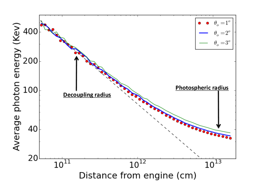
Figure 5.— Radial profile of the average photon energy from a test MCRaT simulation with a spherical flow. Red marks and colored solid lines show the radial evolution of the photon mean energy at the observing angles $\theta_{o}=1$, 2, and 3 degrees. A dashed line shows the average energy of photons in equilibrium with the plasma. The location of the photosphere and of the radius at which the radiation and plasma decouple according to Giannios (2012) are shown with vertical arrows.

As a second test we run a suite of simulations of spherical outflows, i.e., outflows with only outward radial velocity component. In this case, the Lorentz factor increases proportionally to the radius until all the internal energy is converted into bulk motion, saturation is reached, and the fireball transitions from accelerating to coasting at constant Lorentz factor. In the acceleration stage the electrons’ temperature decreases proportionally to $r^{-1}$; as the asymptotic Lorentz factor is reached, the fireball coasts at constant $\Gamma$ and the electrons’ temperature decreases as $r^{-2/3}$. We stress that this analytical solution was imposed, we did not run a hydrodynamic simulation of a spherical outflow, we simply replaced the output of the simulation with the analytical prescription.

We first compare the photon luminosity of the spherical fireball calculated from the simulations with the analytical expectation. The result is shown in Figure 3, where the MCRaT luminosity for four different observers is compared to the analytical expectation. While for observers away from the singular polar axis we find good agreement, a deviation of $\sim 20$ per cent is observed at $\theta_{0}=0.5^{\circ}$. We ascribe this to the artifact of the polar axis. Since the polar axis is singular in the coordinate system, the weight of photons close to the axis can be very small (cfr. Eq. 1). For infinite number of photons, all small angles are sampled and there is no systematic deviation in the results. For a finite number of photons, however, significant non-Poissonian deviations can result from under- or oversampling the smallest polar angles. An analogous effect can be seen in Figure 8 of Morsony et al. 2007 (dashed line) where an unphysical drop of the luminosity is observed at small polar angles from the jet axis. In the remainder of this manuscript we will compute light curves and spectra only for photons propagating with a polar angle of at least $0.5^{\circ}$ to avoid this problematic region.

In Figure 4 we show the time-integrated spectrum accumulated between angles $\theta_{o}=1$ and 2 degrees from the polar axis. The spectrum is broader than a Planck function, and agrees very well with the prediction of Goodman (1986). Finally, we show in Figure 5 the radial dependence of the average photon energy for various off-axis angles compared to the average frequency of photons in equilibrium with the fluid. As described in great detail in Beloborodov (2011; see e.g. their Figure 3), the photon temperature follows the electron temperature at large optical depth $\tau>10$. As the photosphere is approached, the electrons and photons decouple and the photons start to cool at a slower rate until, at the photosphere, the decoupling of the radiation is complete and the photon temperature remains constant. The MCRaT result is shown in Figure 5. Red symbols and colored lines show the average photon energy for viewing angles $\theta_{o}=1$, 2, and 3^∘. A dashed line shows instead the average energy of photons strongly coupled to the electrons. Two vertical arrows show the location of the photosphere and the location at which the Giannios (2012) condition is attained (the Wien radius, Beloborodov 2013). The MCRaT result reproduces all the features of the analytical solution (Beloborodov, 2011) and confirms that the approximations adopted so far for computing the peak energy of the prompt GRB spectrum from simulations are inaccurate. While it is true that electrons and photons start decoupling at or around the Wien radius, the decoupling is incomplete and the spectrum keeps cooling by interaction with the electrons. This approximation was adopted in L13 and as a consequence their results overestimate both the light curve luminosity and the peak frequency of the spectrum. On the other hand, the assumption that the electrons and photons are coupled until the photosphere is reached is also incorrect. This approximation, adopted by (Lazzati et al., 2009, 2011; Mizuta et al., 2011; Nagakura et al., 2011) underestimates the radiation peak frequency and the light curve luminosity. A correct implementation of the radiation transfer in numerical simulations of the photospheric model is therefore necessary not only to obtain the spectral properties beyond the peak frequency (the low- and high- frequency spectral indices), but also to correctly estimate the peak frequency itself. Before showing the MCRaT results for a GRB simulation, we stress that within the viewing angles presented in this paper the code is quite accurate, the photon average energies differing only by a few per cent for different lines of sight (Figure 5).

3. Results

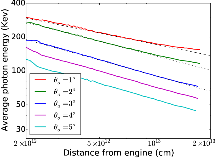
Figure 6.— Radial profile of the average photon density for radiation propagating at different off-axis angles. Analogous to Figure 5 but for the GRB jet simulation. Guidelines are plotted for off-axes 1, 2, and 3 degrees, to show the deviation from the self-similar behaviour as the photosphere is approached (or lack thereof).

We have applied the MCRaT code to our fiducial simulation of a long duration gamma-ray burst jet that was previously studied in the approximation of a sharp photosphere (Lazzati et al. 2009, 2011; L13). The simulation runs for $\sim 600$ s, at which time the jet head has reached a distrance of $\sim 1.3\times 10^{13}$ cm from where it was launched, the center of the progenitor star. The progenitor is modeled as a 16 solar mass Wolf Rayet star, model 16TI from Woosley & Heger (2006). The jet is injected as a boundary condition at $r_{0}=10^{9}$ cm, with luminosity $L=5.33\times 10^{50}$ erg s^-1, half-opening angle $\theta_{0}=10^{\circ}$, Lorentz factor $\Gamma_{0}=5$, and internal energy to allow for an asymptotic jet acceleration to a terminal Lorentz factor $\Gamma_{\infty}=400$. After $t=100$ s, the engine luminosity is decreased by a factor 1000 to simulate the turn off of the engine. The radial resolution at $R=10^{13}$ cm, where the photosphere is expected to lay, is $\delta y=10^{9}$ cm, giving $\delta y/y=10^{-4}$, comparable to $1/\Gamma^{2}$. Resolution in the orthogonal $x$ coordinate is identical since we use square resolution elements. Shocks at the photospheric radius are therefore poorly resolved. Still, this resolution is about an order of magnitude better than in the simulations of Ito et al. (2015). As we discuss below, limited resolution is a serious concern for these results and an increase by at least an order of magnitude is required to ensure that shocks are resolved and that the simulations capture the temperature variations that they produce. 300,000 photons were injected in the simulation at off-axis angles $\theta_{i}\leq 6^{\circ}$.

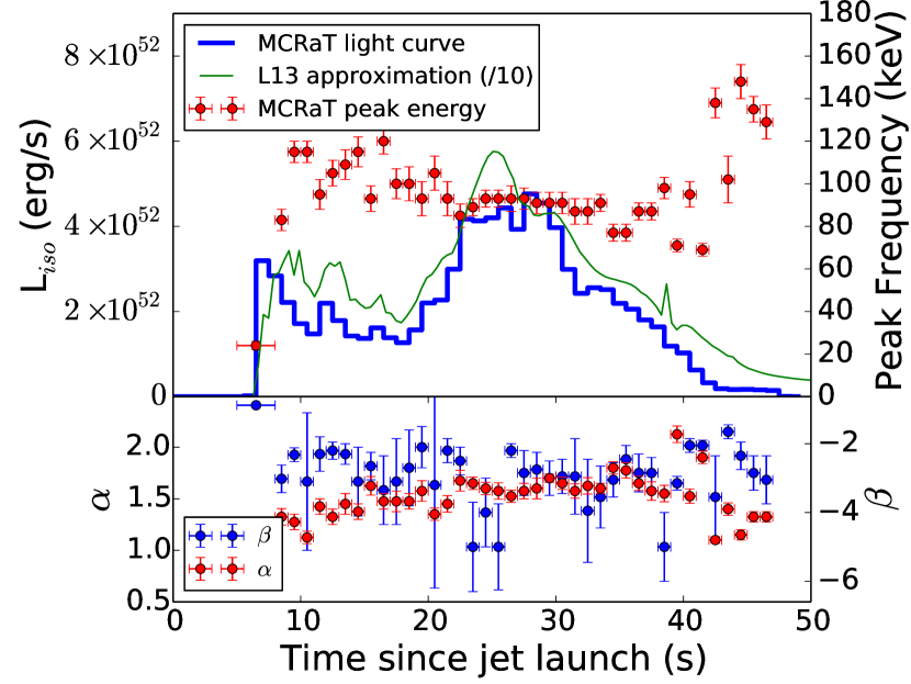
Figure 7.— Light curve and spectral evolution for photons traveling within the acceptance range $0.5\leq\theta_{\rm{ph}}\leq 1.5$ (for an observer laying at $\theta_{o}=1^{\circ}$) from the polar axis. In the upper panel, the thick solid line shows the MCRaT result, the thin line shows the result from L13 (rescaled by a factor 10) and the symbols show the peak energy in 1 second temporal bins (energy y-axis to the right). In the bottom panel, the Band parameters $\alpha$ and $\beta$ are shown with red and blue symbols, respectively. The $\alpha$ scale is to the left, while the $\beta$ scale is to the right.

Under conical expansion, the jet we input in the simulations would become optically thin (and therefore have its photosphere) at $R=6.4\times 10^{11}$ cm (e.g., Mészáros & Rees 2000). However, the progenitor-jet interaction induces a non-conical expansion and prevents the saturation of the acceleration at $\Gamma=400$, resulting in a much larger photospheric radius. Lazzati et al. (2011) found a photospheric radius of the order of $R=10^{13}$ cm in the same simulation, increasing for larger off-axis angles. With MCRaT we do not compute the photospheric radius by integrating the optical depth (as is done in all previous numerical simulations of photospheric emission in GRBS); we follow instead the photon propagation. Whether the photons have crossed the photospheric radius or not can be understood by looking at the radial dependence of their average energy. The average photon energy decreases at radii smaller than the photosphere and attains an asymptotic value beyond it (Beloborodov 2011; see also Section 2.1). In Figure 6 we show the time-averaged MCRaT results for off-axis angles of 1, 2, 3, 4, and 5 degrees, each with an acceptance of $\pm 0.5$ degrees. Analogously to Figure 5, dashed lines are overlaid to show the average frequency of photons coupled to the electrons. The colored lines detach from the dashed ones at the Wien radius and become constant beyond the photospheric radius. In agreement with results obtained from integration over the optical depth (Lazzati et al. 2011, see their Figure 2), we find that the photosphere lies at $R_{\rm{ph}}\sim 1.5\times 10^{13}$ cm for small off-axis angles but is located beyond the outer edge of the simulation box (which is located at $2.5\times 10^{13}$ cm) for relatively large off axis angles $\theta_{o}>3^{\circ}$. In mode detail, the photosphere is clearly reached for $\theta_{o}=1^{\circ}$, is almost reached for $\theta_{o}=2^{\circ}$, and it is approached for $\theta_{o}=3^{\circ}$. In the following we show results for these three off-axis angles, keeping in mind that the result for $\theta_{o}=3^{\circ}$ might be approximate since the simulations do not appear to be extended enough to completely reach the photosphere. It should be remembered, however, that the photosphere is not at a constant distance throughout the simulation, starting at a large radius and progressively closing in (see, e.g., the blue lines in Figure 4 of L13). Even for the larger off-axis angles, the photosphere is likely reached at some time after the initial high-density plug at the jet’s head is overcome.

3.1. Light Curves and Spectra

Light curves and spectra are computed by binning the photons within the acceptance angle in time and/or frequency, each multiplied times its weight (Eq. 1). Light curves for $0.5\leq\theta_{\rm{ph}}\leq 1.5$, $1.5\leq\theta_{\rm{ph}}\leq 2.5$, and $2.5\leq\theta_{\rm{ph}}\leq 3.5$ degrees are shown as thick lines in Figures 7, 8, and 9, respectively. The bin time is one second in all cases. In Figures 7 and 9 a thin line shows the light curves computed with the sharp last energy surface approximation by L13 (see also Giannios 2012). Normalization factors of 10 and 4 were applied to the two curves, respectively, to facilitate the comparison. The MCRaT curves have similar temporal evolution compared to the old sharp approximation. This is not surprising since the light curve shape is mainly due to the hydrodynamic effect of recollimation that the progenitor star imprints on the jet. Such effect is purely hydrodynamic in nature and is therefore independent of how the photon propagation is treated in post-processing. The difference in normalization is due to the fact that, as seen in Figures 5 and 6, the average photon frequency decreases after the last energy exchange radius assumed in L13.

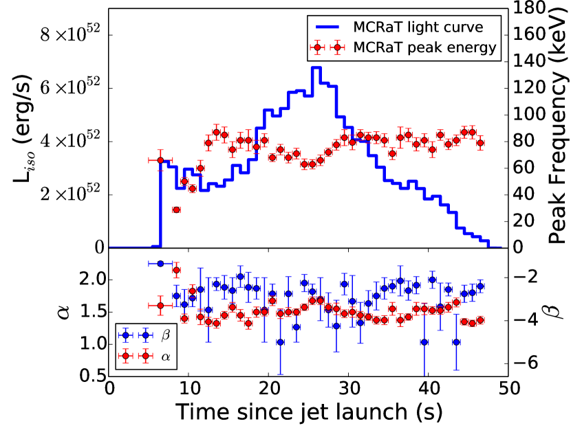
Figure 8.— Same as Figure 7 but for an acceptance angle $1.5\leq\theta_{\rm{ph}}\leq 2.5$. L13 results at this angle are not available for comparison.

A few example spectra for the $1.5\leq\theta_{\rm{ph}}\leq 2.5$ case are shown in Figure 10. We have chosen this case because it is far enough from the jet axis to avoid spurious effects from the reflective symmetry along the y-axis. In addition, as shown in Figure 6, the photospheric radius is contained in our simulations at this off-axis angle. The three panels show the photon count spectra for the whole burst (left panel), a fairly non-thermal time interval (central panel), and the most luminous time bin of the light curve (left panel). In all cases we notice some features in agreement with observed gamma-ray bursts and others in significant tension with the observations. All spectra are fit with a Band model (Band et al., 1993) and the best values for the parameters $\alpha$, $\beta$, and $h\nu_{\rm{pk}}$ are reported. In the Band model, a smoothly joined broken power-law function, $\alpha$ is the asymptotic photon index at low frequency, $\beta$ is the asymptotic photon index at high frequency, and $h\nu_{\rm{pk}}$ is the photon energy at which the $\nu F(\nu)$ spectrum peaks.

Going from low- to high-frequencies, we first notice that the low-energy spectral index $\alpha$ is found to be significantly larger than in observations. Average observed values of $\alpha$ range between -1 and -0.5 (Preece et al., 2000; Goldstein et al., 2013; Gruber et al., 2014; Yu et al., 2016) while we consistently find $\alpha>1$. This is not surprising since the difficulty of the photospheric model to reproduce the observations in the low-frequency range is well known. Our synthetic spectra have power-law indices even steeper than a black body, due to the fact that the spectrum was injected with a Wien distribution of frequencies. Injecting a black body spectrum would have made the low-frequency spectrum harder, however the steepening of the spectrum would not have bee substantial enough to reproduce the typical spectra of GRB observations. We also notice that our simulations do not test any of the solutions proposed to solve the discrepancy. For example, models based on sub photospheric dissipation (e.g. Chhotray & Lazzati 2015) can be tested only with simulations of higher resolution than the one presented here, since shocks need to be fully resolved to affect the radiation spectrum. Models based on the addition of soft photons from synchrotron (Vurm et al., 2011; Vurm & Beloborodov, 2015) require instead a radiation transfer code that allows for photon emission and absorption, beyond the current capabilities of MCRaT.

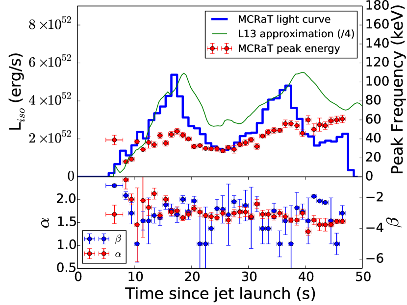
Figure 9.— Same as Figure 7 but for an acceptance angle $2.5\leq\theta_{\rm{ph}}\leq 3.5$.

The peak energy of the light curves is found in the $\sim 100$ keV range. This is a fairly common value for a burst of intermediate luminosity like the one simulated here. Yet, it is on the low tail of the distribution and we will see in Section 3.2 that there is some strain between our results and the Amati and Yonetoku correlations.

The best agreement between our results and observations is found at high frequencies. We first notice that we can exclude both a cutoff power-law and a Black Body fit withs high confidence. A $\chi^{2}$-based F-test yields probabilities $P<10^{-5}$ for the two simpler functions mentioned above to give a comparable fit with respect to a Band Function. A high-frequency power-law is therefore required by the data, as in observed bursts. In addition, we find that MCRaT’s $\beta$ values, between 2 and 3, are fairly typical for long-duration GRBs (Preece et al., 2000; Goldstein et al., 2013; Gruber et al., 2014; Yu et al., 2016). We note that the spectra shown only extend to $\sim 1MeV$ due to poor statistics, but there is no indication of a cutoff. In the left panel – the one with the best statistics – we show with smaller symbols and in grey color the data in the spectral bins that have too little photons to be included in the fit. We notice that these data points are consistent with the extrapolation of the high-frequency power-law and no break or cutoff is required. Very high frequency photons in the GeV band detected by Fermi (Abdo et al., 2009) are however better explained as forward shock emission in the photospheric model (Kumar & Barniol Duran, 2009; Ghisellini et al., 2010).

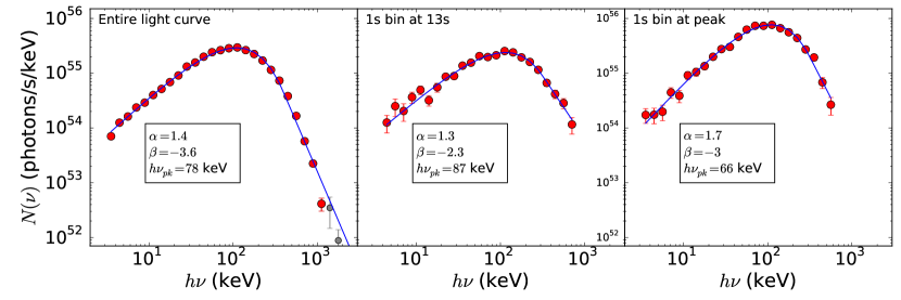
Figure 10.— Sample MCRaT photon-count spectra for the $1.5\leq\theta_{\rm{ph}}\leq 2.5$ observer. The left panel shows the spectrum accumulated over the entire light curve and fit with a Band model. The central panel shows one of the most non-thermal spectrum, accumulated over a 1 s time bin at $t=13$ s. Finally, the left panel shows the spectrum at the light curve peak. Each panel shows the best fit Band parameters in an inset and the best fit Band spectrum as a thin solid line. In the left panel bins with some photon counts but not enough statistics to be included in te fit are shown in gray and with a smaller size.

Figures 7, 8, and 9 show, besides the light curves, the results of time-resolved spectroscopy. Photons were accumulated in 1 s bins and a Band spectrum was fit to each temporal bin and for each of the three off-axis observers. The top panel of each figure reports the peak energy in keV (right hand vertical scale), while the bottom panel reports the best fit $\alpha$ and $\beta$ values. The low-frequency index $\alpha$ refers to the left hand vertical scale, while the high-frequency index $\beta$ refers to the right hand vertical scale. We first notice that there is quite some diversity in the kind of spectral evolution observed in the three figures. At small off-axis $\theta_{o}=1^{\circ}$, the peak frequency follows a general hard-to-soft trend, while the low-frequency index $\alpha$ has a small growing trend. Eventually, both trends are broken. At times larger than $t\sim 40$ s the peak energy rises above 100 keV while the spectral index $\alpha$ fluctuates with no stable trend. This transition is due to the emergence of the unshocked jet, as already seen in previous simulations (Morsony et al. 2007; Lazzati et al. 2009; L13). The hard-to-soft trend has been observed in some bursts. The $\alpha$ increase, on the other hand is not observed but seem irrelevant since, as already noted above, our spectra have $\alpha$ indices in significant disagreement with observations.

Moving away form the axis, at $\theta_{o}=2^{\circ}$ we find a light curve with very little spectral evolution, except for an initial hardening and a small softening around the peak. This is quite unusual in observations. Finally, at $\theta_{o}=3^{\circ}$ we find an example of tracking behavior, the peak energy increasing at high luminosity and decreasing at low luminosity. Again, towards the end of the burst a global hardening is observed, possibly due to the emergence of the unshocked jet or to the fact that photons at the end of the burst haven’t yet reached the photosphere. In all three cases, non-thermal high-energy tails are measured throughout the burst, with the exception of a few intervals in which the high-frequency index was fixed to $\beta=-5$.

We stress that the jet input in the simulation has constant luminosity and any variation in the light curve luminosity is brought about by the jet-progenitor interaction. There is evidence that variability is injected at the base of the jet (Morsony et al., 2010). More pronounced spectral evolution is expected for burst with variable central engines (López-Cámara et al., 2014). In addition, the simulations we present here might have engines that are active for too long a time, as pointed out in Lazzati et al. (2013b).

3.2. Correlations

One of the reasons for the success of the photospheric model was its ability to reproduce the Amati, Yonetoku, Golenetskii, $E_{\rm{iso}}-\Gamma$, and energy-efficiency correlations (Golenetskii et al., 1983; Amati et al., 2002; Yonetoku et al., 2004; Liang et al., 2010; Ghirlanda et al., 2012). This was demonstrated with the results of numerical simulations, and the scaling was ascribed principally to a line of sight effect (L13). With MCRaT we can re-analyze the success of the photospheric model in reproducing the observational ensemble correlations. We show in Figure 11 the result for the Yonetoku correlation between the 1-s binned peak luminosity and the peak frequency measured at the time of the peak (again, integrated over 1 s). Given the results shown above, it does not come as a surprise that the MCRaT result are not a perfect match to the observations. The assumption of a complete decoupling at the Wien radius adopted by L13 (see also Giannios 2012) is indeed fairly crude. While it is true that the radiation decouples from the leptons at that optical depth, the radiation continues to cool, even though remaining at a temperature that is higher than that of the matter (Beloborodov 2011; see also Figure 5). As a consequence, the MCRaT spectra peak at a frequency that is too low by a factor $\sim 3$ with respect to observations. Such an offset is not large enough to reject the model, since the dispersion of the data is comparable, yet it puts the simulation results at some strain with the data. Analogous results hold for all the aforementioned correlations, with the exception of the $E_{\rm{iso}}-\Gamma$ and energy-efficiency correlations, for which no significant discrepancy is found. The agreement, however, is most likely due to the poor definition of the correlations in the data rather than to a true success of the model.

4. Summary and discussion

We have presented a novel numerical code to perform Monte Carlo radiation transfer in relativistic jets under the assumption that the radiation-matter interaction is dominated by Compton scattering off the leptons in the fluid. Our code is analogous to the one recently developed by Ito et al. (2013, 2015) and we find similar results, even though they applied it to a different set of simulations. Neither MCRaT nor the Ito et al. (2013, 2015) code cannot take into account the radiation feedback on the hydrodynamics. However, the hydrodynamic simulations to which the Monte Carlo codes are applied assume infinite coupling (the equation of state for both photons and plasma are the same) and therefore the dynamics from the HD simulations should be accurate in the optically thick part of the outflow, where most of the Compton scatterings take place and the spectrum takes its shape. Despite these limitations, both MCRaT and the Ito et al. code constitute a significant advance over previous studies, in which the coupling between matter and radiation was assumed to be complete at optical depths larger than a critical value and null at smaller optical depths. Said critical optical depth was assumed to be either unity (Lazzati et al., 2009, 2011; Mizuta et al., 2011; Nagakura et al., 2011), or of several tens (Giannios 2012; L13). As analytically predicted for spherical outflows by Beloborodov (2011), proper radiation transfer shows that the radiation and matter indeed start to decouple at an opacity of several tens. However, the radiation keeps cooling significantly until the photosphere is reached, at which point the radiation propagates with constant average properties. In addition, MC radiation transfer allows for a full calculation of the emitted spectrum, while only its peak frequency could be estimated under the approximations previously employed.

We have applied MCRaT to our fiducial GRB jet simulation, used in previous photospheric work. We find that the MCRaT results predict light curves that are dimmer and characterized by lower frequency photons with respect to the results from L13. Spectral and temporal analysis was performed on the resulting light curves and spectra. We find that, as predicted by many analytical and semi-analytical previous publications, photospheric radiation is characterized by a significant non-thermal high-frequency tail. Fitting the time-resolved spectra with a Band function we find values of the index $\beta$ in good agreement with the observations and a significant evolution of the slope over the burst light curve. Because of the continued radiation cooling in the sub-photospheric region, we find that the MCRaT spectra are characterized by photons of lower frequency with respect to the L13 results. This deteriorates the agreement of the simulation results with the Amati and Yonetoku ensemble correlations. While the MCRaT results are still within the observed dispersion, they do not follow the correlation closely and more work is necessary to better understand the role of photospheric emission in the establishment of such correlations. In addition, we find that our simulations do not reach the photospheric radius for off-axis angles $\theta_{o}>2^{\circ}$, preventing the analysis of the off-axis light curves that were deemed to be responsible for the correlations (L13). We also find that the low-frequency spectral index is much steeper than observed. This is a well known problem of photospheric emission in the absence of an efficient emission mechanism or of strong sub-photospheric dissipation and the discrepancy found is not surprising.

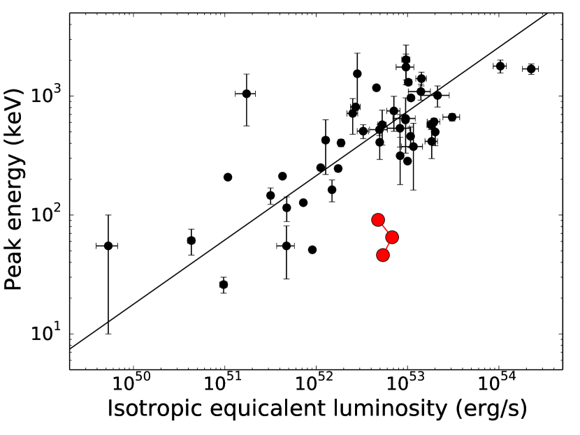
Figure 11.— Comparison between the observational Yonetoku correlation (black symbols with error bars and best fit solid line) with the MCRaT results (red symbols).

One possible shortcoming of this work that could be at the basis of the discrepancies discussed above is the resolution of the simulations. In order to study the effect of shock-heating on the spectrum we need to be able to resolve the shocks so that their true temperature can be taken into account. Unfortunately, the resolution of the simulations presented here is sufficient only to moderately resolve the shocks. As a consequence, continuous heating from recombination, or the kind of shock heating envisaged in, e.g., Chhotray and Lazzati (2015), could not be studied. We plan to perform higher-resolution simulations for both long and short GRB jets in the near future to test the impact of resolution on the results. Some hope comes from the comparison of our results with those of Ito et al. (2015). Their resolution is lower than ours, but they consider precessing jets that substantially increase dissipation. Even though they do not perform a detailed time-resolved analysis of their spectra, it is clear from their Figures 3 and 4 that significant non-thermal features at both ends of the spectrum can be obtained. In addition, we stress that the simulation presented here injects a constant luminosity from the inner engine and does not have, therefore, internal shocks. Realistic engines are likely characterized by intrinsic variability, and a better agreement with the Amati and Yonetoku ensemble correlations could be obtained from a light curve with the same peak frequency and peak luminosity but with periods of very weak emission.

Additional physics might also be required to obtain a better match of the synthetic spectra with observations. Shocks likely inject non-thermal particles that are neglected by MCRaT and by the Ito et al. (2015) code alike. Magnetic fields and the possibility of injection of soft photons from synchrotron are also ignored (Vurm et al., 2011; Vurm & Beloborodov, 2015). Additional dissipation is also provided by magnetic reconnection (Giannios & Spruit, 2007; McKinney & Uzdensky, 2012). While adding such effects would not be trivial, breaking the embarrassingly parallel structure of the code and making the whole calculation longer, it is not impossible and we are currently developing a version of the MCRaT code that takes into account non-thermal particles and synchrotron emission. Since all the missing effects are likely to increase the non-thermal aspect of the spectrum, our the results presented here can be seen as a lower limit on the non-thermal features of the photospheric spectrum from GRB jets.

Finally, we would like to comment on the fact that in no case we found the need to add a low-temperature thermal component to the spectral model used to fit our spectra. Yet, such a component has been detected in several bursts and is considered one of the proofs of the existence of a photospheric contribution to the GRB prompt spectrum (Guiriec et al., 2011; Ghirlanda et al., 2013; Guiriec et al., 2013; Burgess et al., 2014; Nappo et al., 2016). Our results, as well as Ito’s results seem to show that the appearance of the photospheric component is always non-thermal and at significantly higher frequencies than those at which the thermal components are detected (typically a few keV to a few tens of keV). The thermal peaks detected in BATSE and Fermi observations are therefore either arising from a different component of the outflow that is not present in the simulations or are a signature of a weak photosphere in a jet dominated by non-thermal and/or non-baryonic energy, such as in a Poynting dominated outflow.

Appendix A Derivation of the photon weight

The luminosity of a uniform jet can be written as (e.g., Morsony et al. 2010):

$$L_{j}=\Omega_{j}R^{2}\left(4p+\rho^{\prime}c^{2}\right)\Gamma^{2}c$$ (A1)

where $p$ is the pressure of the jet material, and $\rho^{\prime}$ its comoving density. For a jet dominated by radiation ($p=aT^{\prime 4}/3$, and $p\gg\rho^{\prime}c^{2}$), and considering the solid angle of a one-sided jet, the equation simplifies to:

$$L_{j}=\frac{8\pi}{3}\left(1-\cos\theta_{j}\right)R^{2}aT^{\prime 4}\Gamma^{2}c$$ (A2)

Deriving with respect to the polar angle we find the luminosity per unit polar angle (the simulated quantity in cylindrical symmetry) and dividing by the average photon energy $h\bar{\nu}=\Gamma h\bar{\nu}^{\prime}$ we obtain the number of photons per unit polar angle as:

$$\frac{dN_{\gamma}}{dt\,d\theta}=\frac{1}{h\bar{\nu}}\frac{dL}{d\theta}=\frac{8\pi}{3}\sin\theta_{j}R^{2}\frac{aT^{\prime 4}}{h\bar{\nu}^{\prime}}\Gamma c=\frac{8\pi}{3}\sin\theta_{j}R^{2}n_{\gamma}^{\prime}\Gamma c=\frac{8\pi}{3}\sin\theta_{j}R^{2}\xi T^{\prime 3}\Gamma c$$ (A3)

This should be equal to the number of photons we inject in the simulation times the weight assigned to each photon:

$$\frac{dN_{\gamma}}{dt\,d\theta}=\frac{w_{\gamma,i}N_{\rm{inj}}}{\delta t\,\delta\theta}$$ (A4)

Solving for $w_{\gamma,i}$ yields Eq. 1.

References

- Abdo et al. (2009) Abdo, A. A., Ackermann, M., Arimoto, M., et al. 2009, Science, 323, 1688
- Abramowicz et al. (1991) Abramowicz, M. A., Novikov, I. D., & Paczynski, B. 1991, ApJ, 369, 175
- Amati et al. (2002) Amati, L., Frontera, F., Tavani, M., et al. 2002, A&A, 390, 81
- Band et al. (1993) Band, D., Matteson, J., Ford, L., et al. 1993, ApJ, 413, 281
- Beloborodov (2010) Beloborodov, A. M. 2010, MNRAS, 407, 1033
- Beloborodov (2011) Beloborodov, A. M. 2011, ApJ, 737, 68
- Beloborodov (2013) Beloborodov, A. M. 2013, ApJ, 764, 157
- Beloborodov (2016) Beloborodov, A. M. 2016, arXiv:1604.02794
- Burgess et al. (2014) Burgess, J. M., Preece, R. D., Connaughton, V., et al. 2014, ApJ, 784, 17
- Chhotray & Lazzati (2015) Chhotray, A., & Lazzati, D. 2015, ApJ, 802, 132
- Daigne & Mochkovitch (1998) Daigne, F., & Mochkovitch, R. 1998, MNRAS, 296, 275
- Daigne et al. (2011) Daigne, F., Bošnjak, Ž., & Dubus, G. 2011, A&A, 526, A110
- Ghirlanda et al. (2012) Ghirlanda, G., Nava, L., Ghisellini, G., et al. 2012, MNRAS, 420, 483
- Ghirlanda et al. (2013) Ghirlanda, G., Pescalli, A., & Ghisellini, G. 2013, MNRAS, 432, 3237
- Ghisellini et al. (2010) Ghisellini, G., Ghirlanda, G., Nava, L., & Celotti, A. 2010, MNRAS, 403, 926
- Giannios (2006) Giannios, D. 2006, A&A, 457, 763
- Giannios & Spruit (2007) Giannios, D., & Spruit, H. C. 2007, A&A, 469, 1
- Giannios (2012) Giannios, D. 2012, MNRAS, 422, 3092
- Goldstein et al. (2013) Goldstein, A., Preece, R. D., Mallozzi, R. S., et al. 2013, ApJS, 208, 21
- Golenetskii et al. (1983) Golenetskii, S. V., Mazets, E. P., Aptekar, R. L., & Ilinskii, V. N. 1983, Nature, 306, 451
- Goodman (1986) Goodman, J. 1986, ApJ, 308, L47
- Gruber et al. (2014) Gruber, D., Goldstein, A., Weller von Ahlefeld, V., et al. 2014, ApJS, 211, 12
- Guiriec et al. (2011) Guiriec, S., Connaughton, V., Briggs, M. S., et al. 2011, ApJ, 727, L33
- Guiriec et al. (2013) Guiriec, S., Daigne, F., Hascoët, R., et al. 2013, ApJ, 770, 32
- Ito et al. (2013) Ito, H., Nagataki, S., Ono, M., et al. 2013, ApJ, 777, 62
- Ito et al. (2014) Ito, H., Nagataki, S., Matsumoto, J., et al. 2014, ApJ, 789, 159
- Ito et al. (2015) Ito, H., Matsumoto, J., Nagataki, S., Warren, D. C., & Barkov, M. V. 2015, ApJ, 814, L29
- Kumar & Barniol Duran (2009) Kumar, P., & Barniol Duran, R. 2009, MNRAS, 400, L75
- Lazzati et al. (2009) Lazzati, D., Morsony, B. J., & Begelman, M. C. 2009, ApJ, 700, L47
- Lazzati & Begelman (2010) Lazzati, D., & Begelman, M. C. 2010, ApJ, 725, 1137
- Lazzati et al. (2011) Lazzati, D., Morsony, B. J., & Begelman, M. C. 2011, ApJ, 732, 34
- Lazzati et al. (2013) Lazzati, D., Morsony, B. J., Margutti, R., & Begelman, M. C. 2013a, ApJ, 765, 103 (L13)
- Lazzati et al. (2013b) Lazzati, D., Villeneuve, M., López-Cámara, D., Morsony, B. J., & Perna, R. 2013b, MNRAS, 436, 1867
- Liang et al. (2010) Liang, E.-W., Yi, S.-X., Zhang, J., et al. 2010, ApJ, 725, 2209
- Lloyd-Ronning & Petrosian (2002) Lloyd-Ronning, N. M., & Petrosian, V. 2002, ApJ, 565, 182
- López-Cámara et al. (2014) López-Cámara, D., Morsony, B. J., & Lazzati, D. 2014, MNRAS, 442, 2202
- Lundman et al. (2013) Lundman, C., Pe’er, A., & Ryde, F. 2013, MNRAS, 428, 2430
- McKinney & Uzdensky (2012) McKinney, J. C., & Uzdensky, D. A. 2012, MNRAS, 419, 573
- Mészáros & Rees (2000) Mészáros, P., & Rees, M. J. 2000, ApJ, 530, 292
- Mizuta et al. (2011) Mizuta, A., Nagataki, S., & Aoi, J. 2011, ApJ, 732, 26
- Morsony et al. (2007) Morsony, B. J., Lazzati, D., & Begelman, M. C. 2007, ApJ, 665, 569
- Morsony et al. (2010) Morsony, B. J., Lazzati, D., & Begelman, M. C. 2010, ApJ, 723, 267
- Nagakura et al. (2011) Nagakura, H., Ito, H., Kiuchi, K., & Yamada, S. 2011, ApJ, 731, 80
- Nappo et al. (2016) Nappo, F., Pescalli, A., Oganesyan, G., et al. 2016, arXiv:1604.08204
- Pe’er et al. (2006) Pe’er, A., Mészáros, P., & Rees, M. J. 2006, ApJ, 642, 995
- Pe’er & Ryde (2011) Pe’er, A., & Ryde, F. 2011, ApJ, 732, 49
- Peer (2015) Pe’er, A. 2015, Advances in Astronomy, 2015, 907321
- Piran (1999) Piran, T. 1999, Phys. Rep., 314, 575
- Preece et al. (2000) Preece, R. D., Briggs, M. S., Mallozzi, R. S., et al. 2000, ApJS, 126, 19
- Rees & Meszaros (1994) Rees, M. J., & Meszaros, P. 1994, ApJ, 430, L93
- Rees & Mészáros (2005) Rees, M. J., & Mészáros, P. 2005, ApJ, 628, 847
- Santana et al. (2016) Santana, R., Crumley, P., Hernández, R. A., & Kumar, P. 2016, MNRAS, 456, 1049
- Vurm et al. (2011) Vurm, I., Beloborodov, A. M., & Poutanen, J. 2011, ApJ, 738, 77
- Vurm & Beloborodov (2015) Vurm, I., & Beloborodov, A. M. 2015, arXiv:1506.01107
- Woosley & Heger (2006) Woosley, S. E., & Heger, A. 2006, ApJ, 637, 914
- Yonetoku et al. (2004) Yonetoku, D., Murakami, T., Nakamura, T., et al. 2004, ApJ, 609, 935
- Yu et al. (2016) Yu, H.-F., Preece, R. D., Greiner, J., et al. 2016, A&A, 588, A135
- Zhang & Yan (2011) Zhang, B., & Yan, H. 2011, ApJ, 726, 90