Efficiently Creating 3D Training Data for Fine Hand Pose Estimation

Abstract

While many recent hand pose estimation methods critically rely on a training set of labelled frames, the creation of such a dataset is a challenging task that has been overlooked so far. As a result, existing datasets are limited to a few sequences and individuals, with limited accuracy, and this prevents these methods from delivering their full potential. We propose a semi-automated method for efficiently and accurately labeling each frame of a hand depth video with the corresponding 3D locations of the joints: The user is asked to provide only an estimate of the 2D reprojections of the visible joints in some reference frames, which are automatically selected to minimize the labeling work by efficiently optimizing a sub-modular loss function. We then exploit spatial, temporal, and appearance constraints to retrieve the full 3D poses of the hand over the complete sequence. We show that this data can be used to train a recent state-of-the-art hand pose estimation method, leading to increased accuracy. The code and dataset can be found at https://github.com/moberweger/semi-auto-anno/.

1 Introduction

Recent work on articulated pose estimation [7, 16, 24, 26, 28] has shown that a large amount of accurate training data makes reliable and precise estimation possible. For human bodies, Motion Capture [7] can be used to generate large datasets with sufficient accuracy. However, creating accurate annotations for hand pose estimation is far more difficult, and still an unsolved problem. Motion Capture is not an option anymore, as it is not possible to use fiducials to track the joints of a hand. Moreover, the human hand has more degrees of freedom than are generally considered for 3D body tracking, and an even larger amount of training data is probably required.

(a)

(b)

(c)

Figure 1: Recent hand pose datasets exhibit significant errors in the 3D locations of the joints. (a) is from the ICVL dataset [26], and (b) from the MSRA dataset [24]. Both datasets were annotated by fitting a 3D hand model, which is prone to converge to a local minimum. In contrast, (c) shows the annotations acquired with our proposed method for the same frame as in (b). (Best viewed in color)

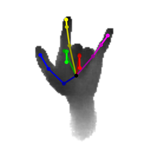
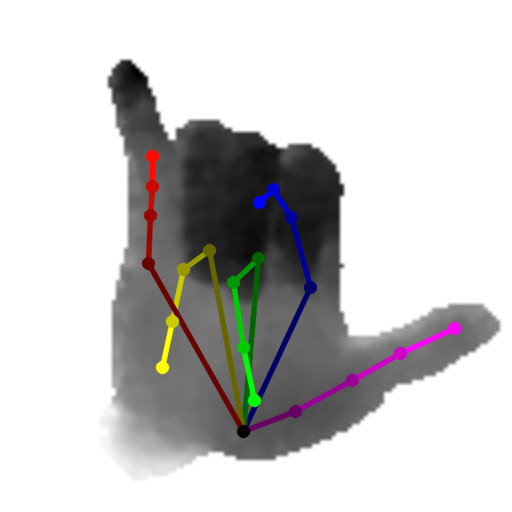
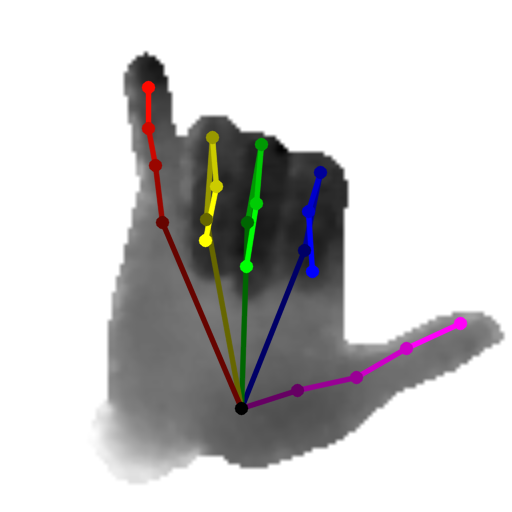
The appearance of depth sensors has made 3D hand pose estimation easier, but has not solved the problem of the creation of training data entirely. Despite its importance, the creation of a training set has been overlooked so far, and authors have had to rely on ad hoc ways that are prone to errors, as shown in Fig. 1. Complex multi-camera setups [2, 23, 28, 29] together with tracking algorithms have typically been used to create annotations. For example, Tompson et al. [28] used a complex camera setup with three RGBD cameras to fit a predefined 3D hand model. Looking closely at the resulting data, it seems that the 3D model was often manually adjusted to fit the sequences better and in between these manually adjusted frames the fit can be poor. Further, the dataset of [26] contains many misplaced annotations, as discussed by [15, 25]. Although recent datasets [24] have paid more attention to high quality annotations, they still contain annotation errors, such as multiple annotations on a single finger, or mixing fingers. These errors result in noisy training and test data, and make training and evaluating uncertain. This issue was addressed recently by [3], which shows that using a robust loss function for training rather than a least-squares one results in better performance.

These problems can be circumvented via using synthetic training data [19, 21, 34]. Unfortunately, this does not capture the sensor characteristics, such as noise and missing data typical of depth sensors, nor the physical constraints that limit the range of possible hand poses [33]. Another common approach to creating training data is using crowd source platforms, such as Amazon Mechanical Turk. In our case, however, the annotations should be in 3D, which makes the task very challenging if done manually, even with a depth sensor: The sensor can only provide the depth of the skin, not the joints themselves, and even this information is not always available in the case of self-occlusion or missing data. Thus, this task does not lend itself to this kind of crowd sourcing with untrained workers. Moreover, whatever the method, one has to recreate new data for each new sensor.

For all of these reasons, we developed a semi-automated approach that makes it easy to annotate sequences of articulated poses in 3D. We ask a human annotator to provide an estimate of the 2D reprojections of the visible joints in frames we refer to as reference frames. We propose a method to automatically select these reference frames to minimize the annotation effort, based on the appearances of the frames over the whole sequence. We then use this information to automatically infer the 3D locations of the joints for all the frames, by exploiting appearance, temporal, and distances constraints. If this inference fails for some frames, the annotator can still provide additional 2D reprojections; by running the global inference again, a single additional annotation typically fixes many frames.

Figure 2: Our method made it possible to create a fully annotated dataset of more than 2000 frames from an egocentric viewpoint, which is considered to be very challenging [20]. (Best viewed in color)

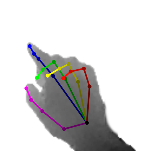
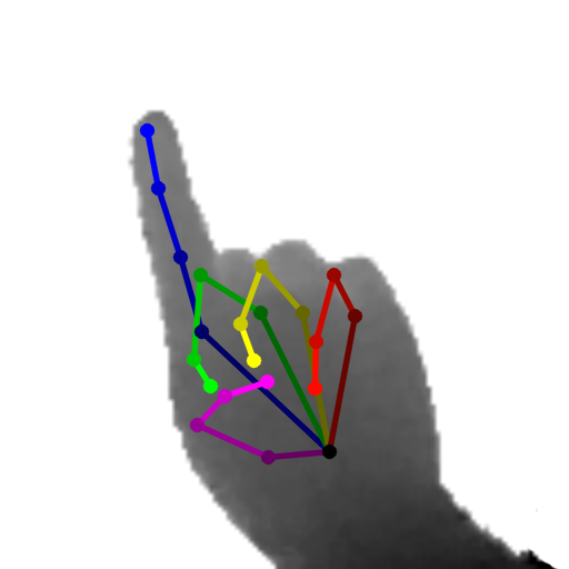
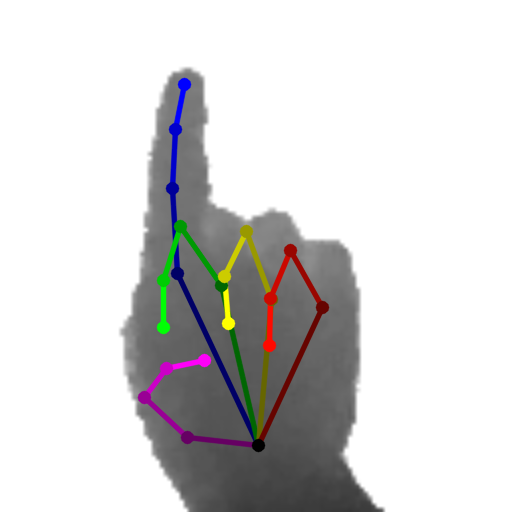
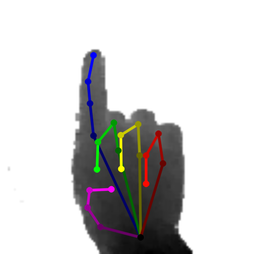
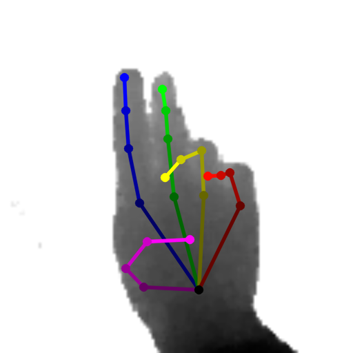
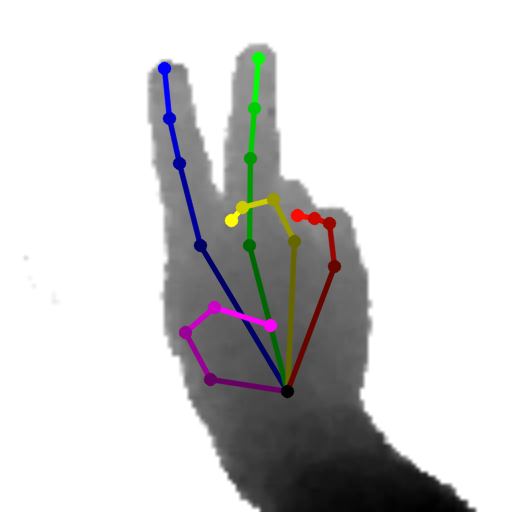
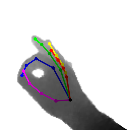
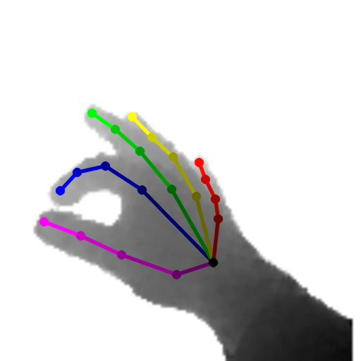
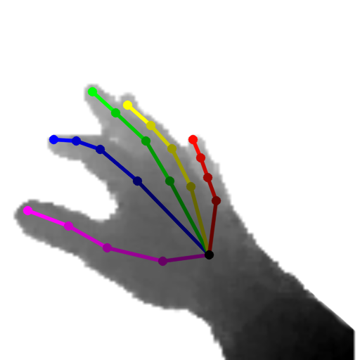
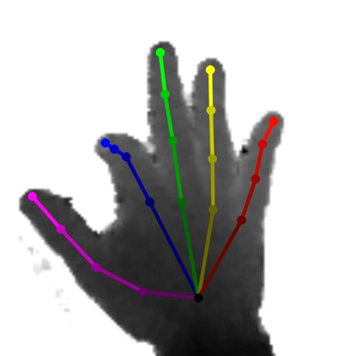
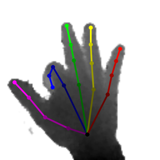
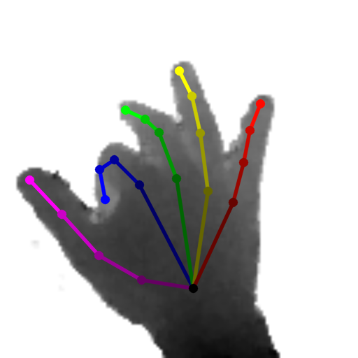
We evaluate our approach using both synthetic data and real images. We also show that we can improve the annotations of existing datasets, which yield more accurate predicted poses. As Fig. 2 shows, our approach also allows us to provide the first fully annotated egocentric sequences, with more than 2000 frames in total. We will make this sequences and the full code available on our website.

2 Related Work

Complex camera setups can be used to mitigate problems with self-occlusions. Tompson et al. [28] relied on three RGBD cameras. They used a predefined 3D hand model that had to be manually readjusted for each person. When looking closely at the data, it appears that the dimensions of the model were modified over the sequences, probably to fit the incoming images better. This dataset was taken from a frontal view of the user, which limits the range of the poses. Sridhar et al. [23] used five RGB and two RGBD cameras, and annotated only the finger tips, which is not enough for full 3D pose estimation. [2, 29] required eight RGB cameras to capture hand interactions, however, causing significant restrictions on hand movement within this setup.

An alternative to these complex setups with restricted ranges are single camera approaches. For example, Tang et al. [26] used the method from [13] to fit a hand model to a single depth image. Similarly, [18, 24] used a single depth camera to fit a predefined 3D hand model. These methods are based on frame-to-frame tracking. This requires manual supervision, and leads to many errors if the optimization does not converge correctly.

Very accurate training data can be generated using synthetic models, as was done in [19, 21, 34] for example. However, synthetic data does not capture the full characteristics of the human hand, and sensor characteristics are not considered. [34] added synthetic sensor noise, however, it is difficult to model this in a general way.

There are also invasive methods for acquiring accurate 3D locations. For example, [32] used a sophisticated magnetic tracker but only for finger tips. [34] used a data glove, but unfortunately data gloves are not very accurate, and would be visible in the training images, thus biasing learning algorithms.

A different approach was proposed by Yasin et al. [35], who matched 2D poses against a set of 3D poses obtained from motion capture sequences, by comparing the 2D poses with the reprojections of the 3D poses in virtual cameras. This is an interesting approach, however, 2D pose estimation is also an open research topic and still prone to errors.

For egocentric 3D hand pose annotation, Rogez et al. [20] proposed a semi-automatic labeling method, where a user labels the 2D locations of a few joints, and chooses the closest 3D pose among a set of synthetic training samples. The 3D pose is then estimated from the 2D annotations and the selected 3D training pose. The user then has to manually refine the pose in 3D. This process is iterated until an appealing result is achieved. This is a time consuming task and thus, they only created a temporally sparse set, which is only sufficient for testing and additional data is required for training.

Semi-automated methods for annotating video sequences like ours are not new to Computer Vision. [10] exploited object silhouettes in reference frames to predict the object silhouettes in the remaining frames. [1] also used manual annotations of some frames to iteratively train a 2D object detector. [31] used annotations in manually selected frames, to predict the annotations of the remaining ones. Compared to these works, we propose a method for selecting the frames to be annotated, minimize manual work, but more importantly, our approach provides a complex articulated 3D structure from 2D annotations.

3 Creating Training Data Efficiently

Given a sequence of $N$ depth maps $\{\mathcal{D}_{i}\}_{i=1}^{N}$ capturing a hand in motion, we want to estimate the 3D joint locations for each $\mathcal{D}_{i}$ with minimal effort. Our approach starts by automatically selecting some of the depth maps we will refer to as reference frames (Section 3.1). A user is then asked to provide the 2D reprojections of the joints in these reference frames, from which we infer their 3D locations in these frames (Section 3.2). We propagate these 3D locations to the other frames (Section 3.3), and we perform a global optimization, enforcing appearance, temporal, and spatial constraints (Section 3.4).

3.1 Selecting the Reference Frames

A simple way to select the reference frames would be to regularly sample the video sequence in time, and select, for example, every tenth frame as reference frame. However, this solution would be sub-optimal: Sometimes the fingers move fast, and a higher sampling rate would be required, while they can also move more slowly, requiring less manual annotation. Moreover, hand motion performers tend to move back to similar poses at wide intervals, and annotating the same poses several times should be avoided.

Simple temporal sampling therefore does not seem to be a good approach. Ideally, we would like to select as few reference frames as possible, while making sure that for each frame, there is at least one reference frame that is similar enough. This will ensure that we can match them together and estimate the joint reprojections in the frame. Let us assume that we know a distance function $d(\mathcal{D}_{i},\mathcal{D}_{j})$ that can be used to evaluate the similarity between two depth maps $\mathcal{D}_{i}$ and $\mathcal{D}_{j}$. Then, the reference frame selection can be formulated as the following Integer Linear Problem (ILP):

$$\operatorname*{arg\,min}_{\{x_{i}\}_{i=1}^{N}}\sum_{i}^{N}x_{i}\quad\text{s.t.}\quad\forall i\>\sum_{j\in E_{i}}x_{j}\geq 1\>,$$ (1)

$$\text{with }E_{i}=\{j\;|\;d(\mathcal{D}_{i},\mathcal{D}_{j})\leq\rho\}\>,$$ (2)

where the $x_{i}$ indicate which frames are selected as reference frames ($x_{i}=1$ if $\mathcal{D}_{i}$ is selected, and 0 otherwise). $E_{i}$ is the set of indices of the frames that are similar enough to frame $i$ for matching, according to distance function $d(\cdot,\cdot)$, and $\rho$ is a threshold.

This formulation guarantees that we find the global optimum. We implemented it using [4] but unfortunately, optimization turned out to be intractable for real problems with the number of frames $N$ larger than about $10^{3}$. Thus, we turned to the suboptimal but tractable approach by optimizing:

$$\max_{\mathcal{R}}\;f(\mathcal{R})\quad\text{s.t.}\quad|\mathcal{R}|<M\>,$$ (3)

where $\mathcal{R}$ is the set of selected reference frames, $M$ the maximum number of reference frames, and $f(\mathcal{R})$ is the number of frames within the chosen distance $\rho$ to at least one of the frames in $\mathcal{R}$. In this approach, if $M$ is set too small, some frames may not have a reference frame near them, but we can trade off the coverage by reference frames with the amount of annotation work. This optimization problem is a submodular problem and it is NP-complete, but what makes it attractive is that a simple greedy optimization was shown to deliver a solution that is close to the globally optimal one [14]. This greedy optimization procedure simply proceeds by adding the element $e$ to the set $\mathcal{R}$ that maximizes the difference $f(e\cup\mathcal{R})-f(\mathcal{R})$ as long as the number of reference frames is smaller than $M$.

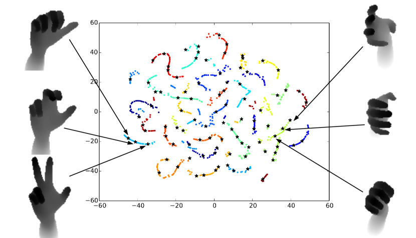
We define the distance function $d(\cdot,\cdot)$ on descriptors computed for depth maps. We tried LINE-MOD [6] and HOG [5]. However, the best results were achieved by cosine distance between low dimensional embeddings computed by a convolutional autoencoder [12]. Fig. 3 shows several examples of reference frames selected with this method, visualized along with the depth map embedding.

Figure 3: t-SNE [30] visualization of the depth map embedding over a sequence. Each colored dot $\bullet$ represents a frame, the color encodes the temporal order. Temporal changes of the hand articulations can be clearly observed from the different trajectories. The reference frames are shown as black stars $\bigstar$. We automatically select them so that their annotations can be propagated to the other frames while minimizing the manual annotation effort. The selected reference frames cover a maximum of other frames within a distance $\rho$, based on their appearance. Note that t-SNE sometimes moves points far apart that are close to each other in the original space. This is why the points do not form a continuous curve even if they correspond to consecutive frames [30]. (Best viewed on screen)

3.2 Initializing the 3D Joint Locations in the Reference Frames

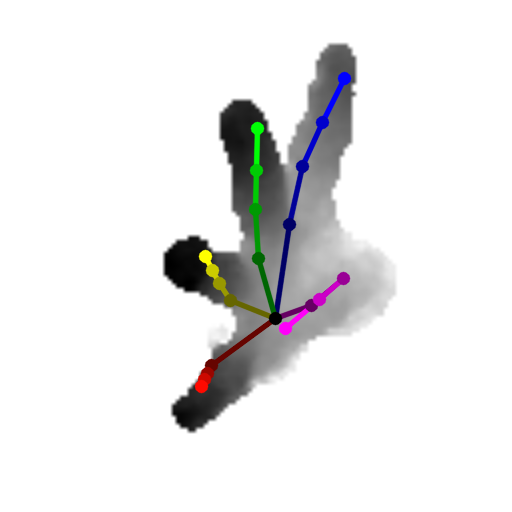
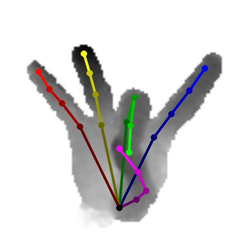
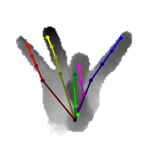
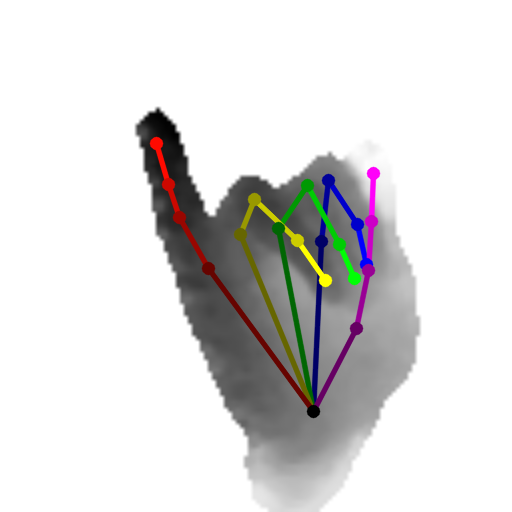
Once the procedure described in the previous section has selected the reference frames, a human annotator has to label them. The annotator is only required to provide the 2D reprojections of the joints with visibility information in each reference frame, and whether these joints are closer or farther from the camera than the parent joint in the hand skeleton tree. This can be done easily and quickly, and we use this information to automatically recover the 3D locations of the joints. It is useful to know the positions of consecutive joints in relation to the camera in order to avoid possible mirroring ambiguities typical of articulated structures [17, 22, 27]. We refer to this information as the z-order constraint.

To automatically recover the 3D locations of the joints, we optimize the following constrained non-linear least squares problem for each reference frame:

$$\operatorname*{arg\,min}_{\{L_{r,k}\}_{k=1}^{K}} \sum_{k=1}^{K}v_{r,k}\lVert\operatorname{proj}(L_{r,k})-l_{r,k}\rVert_{2}^{2}$$ (4)

s.t. $$\forall k\>\>\lVert L_{r,k}-L_{r,p(k)}\rVert_{2}^{2}=d_{k,p(k)}^{2}$$

$$\forall k\>\>v_{r,k}=1\Rightarrow\mathcal{D}_{r}[l_{r,k}]<z(L_{r,k})<\mathcal{D}_{r}[l_{r,k}]+\epsilon$$

$$\forall k\>\>v_{r,k}=1\Rightarrow(L_{r,k}-L_{r,p(k)})^{\top}\cdot c_{r,k}>0$$

$$\forall k\>\>v_{r,k}=0\Rightarrow z(L_{r,k})>\mathcal{D}_{r}[l_{r,k}]$$

where $r$ is the index of the reference frame. $v_{r,k}=1$ if the $k$-th joint is visible in the $r$-th frame, and 0 otherwise. $L_{r,k}$ is the 3D location of the $k$-th joint for the $r$-th frame. $l_{r,k}$ is its 2D reprojection as provided by the human annotator. $\operatorname{proj}(L)$ returns the 2D reprojection of a 3D location. $p(r)$ returns the index of the parent joint of the $k$-th joint in the hand skeleton. $d_{k,p(k)}$ is the known distance between the $k$-th joint and its parent $p(k)$. $\mathcal{D}_{r}[l_{r,k}]$ is the depth value in $\mathcal{D}_{r}$ at location $l_{r,k}$. $z(L)$ is the depth of 3D location $L$. $\epsilon$ is a threshold used to define the depth interval of the visible joints. In practice, we use $\epsilon=15$ mm given the physical properties of the hand. $c_{r,k}$ is equal to the vector $[0,0,-1]^{\top}$ if the $k$-th joint is closer to the camera than its parent in frame $r$, and $[0,0,1]^{\top}$ otherwise. $(L_{r,k}-L_{r,p(k)})$ is the vector between joint $k$ and its parent in this frame.

Together, the terms of Eq. (4) assure that: (1) the bone lengths of the skeleton are respected; (2) visible joints are in range of observed depth values; (3) hidden joints are not in front of observed depth values; and (4) depth order constraints of parent joints are fulfilled. We currently assume that the lengths $d_{k,p(k)}$ are known. In practice, we measure them from a depth map of the hand with open fingers and parallel to the image plane. It may also be possible to optimize these distances as they are constant over the sequences from the same person.

We optimize this problem with SLSQP [8]. Equality constraints are hard to optimize, so we relax them and replace the constraints by a term in the loss function that penalizes constraint violations. We use a simple scheduling procedure to progressively increase the weight of this term. This gives us a reasonable initial estimate of the 3D pose of the hand for each reference frame.

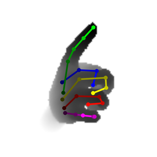
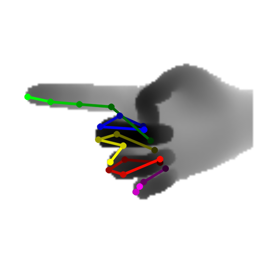
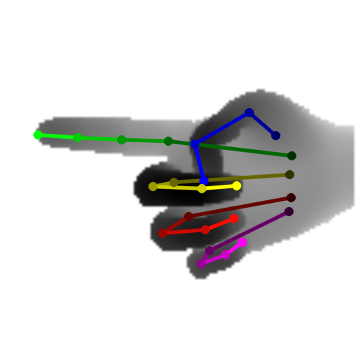
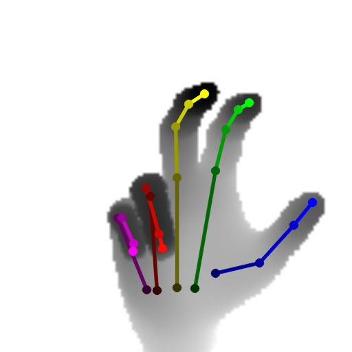
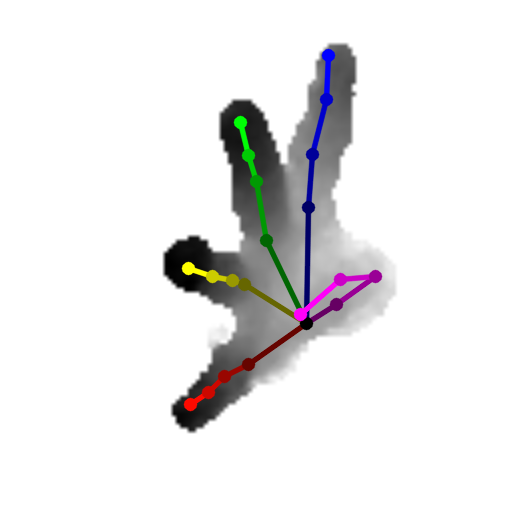
We initialize the joint depth with the measurement from the depth sensor at the annotated 2D location. This is shown in Fig. 4, which depicts the initialized 3D locations and the result after optimizing the relaxation of Eq. (4).

(a) 2D annotation

(b) 3D initialization

(c) 3D result

Figure 4: Optimization steps for reference frames. We start with the 2D annotations on a depth image provided by a user (a), and backproject them to initialize their 3D location estimates. (b) shows the same pose rendered from a different viewpoint, depicting the depth initialization of the joints. We then optimize the constrained non-linear least squares loss of Eq. (4) on these initial 3D locations. The result is shown in (c), again rendered from a different viewpoint, but now with better aligned 3D locations. (Best viewed in color)

3.3 Initializing the 3D Joint Locations in the Remaining Frames

The previous section described how to compute a first estimate for the 3D locations of the joints in the reference frames. Next, we iteratively propagate these 3D locations from the reference frames to the remaining frames, in a way similar to [9], as explained in this section. This gives us an initialization for the joint locations in all the frames. The next subsection will explain how we refine them in a global optimization procedure.

$\mathcal{I}$ is used to denote the set of frames for which the 3D locations of the joints have already been initialized. At the beginning, $\mathcal{I}$ is initialized to the set of reference frames, but each time we estimate the joints for a frame, this frame is added to $\mathcal{I}$. At each iteration, a frame $\hat{c}$ not yet initialized and its closest frame $\hat{a}\in\mathcal{I}$ are selected:

$$\begin{bmatrix}\hat{c}\\ \hat{a}\end{bmatrix}=\operatorname*{arg\,min}_{\begin{subarray}{c}{c\in[1;N]\backslash\mathcal{I}}\\ {a\in\mathcal{I}}\end{subarray}}d(\mathcal{D}_{c},\mathcal{D}_{a})\>.$$ (5)

We use the appearance of the joints in $\hat{a}$ to predict their 3D locations $\{L_{\hat{c},k}\}_{k}$ in $\hat{c}$ by minimizing:

$$\begin{split}\operatorname*{arg\,min}_{\{L_{\hat{c},k}\}_{k}}&\sum_{k}\operatorname{ds}(\mathcal{D}_{\hat{c}},\operatorname{proj}(L_{\hat{c},k});\mathcal{D}_{\hat{a}},l_{\hat{a},k})^{2}\\ \text{s.t.}\quad&\forall k\quad\lVert L_{\hat{c},k}-L_{\hat{c},p(k)}\rVert_{2}^{2}=d_{k,p(k)}^{2}\>,\end{split}$$ (6)

where $\operatorname{ds}(\mathcal{D}_{1},\operatorname{proj}(L_{1});\mathcal{D}_{2},l_{2})$ denotes the dissimilarity between the patch in $\mathcal{D}_{1}$ centered on the projection $\operatorname{proj}(L_{1})$ and the patch in $\mathcal{D}_{2}$ centered on $l_{2}$. This optimization looks for joints based on their appearances in frame $\hat{a}$ while enforcing the 3D distances between the joints. We use the Levenberg-Marquardt algorithm to solve Eq. (6), by relaxing the hard constraint with a weighted additional term in the loss function.

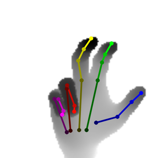
As illustrated in Fig. 5, we initialize the optimization problem of Eq. (6) by aligning frames $\hat{c}$ and $\hat{a}$ using SIFTFlow [11]. This maps the 2D reprojections of the joints in frame $\hat{a}$ to 2D locations $\{\tilde{l}_{k}\}_{k}$ in frame $\hat{c}$. We backproject each $\tilde{l}_{k}$ on the depth map $\mathcal{D}_{\hat{c}}$ to initialize $L_{\hat{c},k}$. If the depth information is missing at $\tilde{l}_{k}$, we use the 3D point that reprojects on $\tilde{l}_{k}$ and with the same depth as $L_{\hat{a},k}$.

(a) Closest reference frame

(b) Initialization with SIFTFlow

(c) After optimization

Figure 5: Initialization of locations on a non-reference frame. (a) shows the 3D locations for the closest reference frame. (b) We propagate the 3D locations using SIFTFlow [11]. (c) 3D locations after optimization of Eq. 6. (Best viewed in color)

3.4 Global Optimization

The previous optimization already gives already a good estimate for the 3D locations of the joints in all frames. However, each frame is processed independently. We can improve the estimates further by introducing temporal constraints on the 3D locations. We therefore perform a global optimization over all the 3D locations $L_{i,k}$ for all the frames by minimizing:

$$\sum_{i\in[1;N]\backslash\mathcal{R}}\sum_{k} \!\operatorname{ds}(\mathcal{D}_{i},\operatorname{proj}(L_{i,k});\mathcal{D}_{\hat{i}},l_{\hat{i},k})^{2}\;+$$

$$\lambda_{M}\sum_{i}\sum_{k} \;\lVert L_{i,k}-L_{i+1,k}\rVert_{2}^{2}\;+$$

$$\lambda_{P}\sum_{r\in\mathcal{R}}\sum_{k} \;v_{r,k}\lVert\operatorname{proj}(L_{r,k})-l_{r,k}\rVert_{2}^{2}\;$$

s.t. $$\forall i,k\quad\lVert L_{i,k}-L_{i,p(k)}\rVert_{2}^{2}=d_{k,p(k)}^{2}\>.$$

The first term (C) sums the dissimilarities of the joint appearances with those in the closest reference frame $\hat{i}=\operatorname*{arg\,min}_{a\in\mathcal{R}}d(\mathcal{D}_{i},\mathcal{D}_{a})$ over the non-reference frames $i$. The second term (TC) is a simple 0-th order motion model that enforces temporal smoothness of the 3D locations. The last term (P) of the sum ensures consistency with the manual 2D annotations for the reference frames. $\lambda_{M}$ and $\lambda_{P}$ are weights to trade off the different terms.

This is a non-convex problem, and we use the estimates from the previous subsection to initialize it. This prevents the optimization from falling into bad local minimums.

This problem has $3KN$ unknowns for $K$ joints and $N$ frames. In practice, the number of unknowns varies from $10^{5}$ to $10^{7}$ for the datasets we consider in the evaluation. Fortunately, this is a sparse problem, which can be efficiently optimized with the Levenberg-Marquardt algorithm.

4 Evaluation

To validate our method, we first evaluate it on a synthetic dataset, which is the only way to have depth maps with ground truth 3D locations of the joints. We then provide a qualitative evaluation on real images, and on the recent MSRA dataset [24]. Finally, we show that we can use our method to create a large dataset of egocentric annotated frames.

4.1 Evaluation on Synthetic Data

We used the publicly available framework of [19] to generate synthetic depth images along with the corresponding ground truth annotation. The sequence consists of 3040 frames, and shows a single hand performing various poses and arm movements. We refer to the supplemental material for videos.

Reference Frame Selection

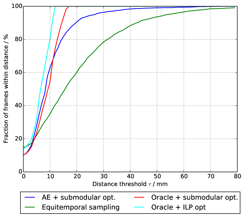
In Fig. 6, we plot the fraction of frames for which the maximum 3D distance of their joints to their locations in the assigned reference frame is lower than a threshold. More formally, we plot the function $n(\tau)$ with:

$$n(\tau):=\frac{1}{N}\Big{|}\Big{\{}i\in[1;N]\;|\;\max_{k}\;\lVert L^{\text{GT}}_{i,k}-L^{\text{GT}}_{a(i),k}\rVert_{2}<\tau\Big{\}}\Big{|}\>,$$ (7)

where the $L^{\text{GT}}_{i,k}$ are the ground truth 3D locations for the joints, and $a(i)=\arg\min_{a\in\mathcal{R}}d(\mathcal{D}_{i},\mathcal{D}_{a})$. This metric allows us to check if the selection based on the visual appearance using distance $d(\cdot,\cdot)$ also retrieves reference frames that are close in 3D. This is an important factor for the rest of the method, as the propagation step will perform better if a frame is not too far away from the closest reference frame. We use $\rho=0.1$, which we obtained by cross-validation, however, the reference frame selection is not very sensitive to the exact value.

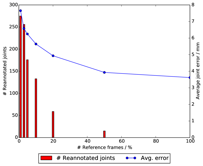
We compare our selection with a straightforward selection based on regular temporal sampling using the same number of reference frames. According to this metric, our method is significantly better, and it actually yields more accurate 3D annotations: Using our proposed selection, the average error is 5.53 mm, compared to 6.45 mm when taking equitemporal samples. Additionally, the required number of manual reannotations is much higher. Our method required 133 additional 2D locations, compared to 276 manual interventions for the equitemporal selection.

Figure 6: Evaluation of the reference frame selection method on the synthetic sequence. We plot the metric $n(\tau)$ of Eq. (7) for our selection of 304 reference frames, and the same number of reference frames sampled regularly in time. With our method, the non-reference frames are closer in 3D to the reference frames. For the oracle, we assume the pose given, and apply the submodular optimization on the Euclidean pose distances. The average pose distance of our proposed selection is only 0.5 mm worse than the oracle. For this sequence, the number of frames is about $10^{3}$, thus solving the ILP is still feasible. The approximation using our submodular optimization is close to the optimal ILP solution, which on average is only 1 mm better. (Best viewed in color)

Reference Frame Initialization

Table 1 provides the accuracy of the initialization of the 3D joint locations for the reference frames, and evaluates the influence of the different terms in Eq. (4). We first use the perfect 2D locations of the joints from ground truth. When only minimizing the 2D reprojection errors with the 3D distance constraints, the error is quite large. Adding the visibility constraint significantly improves the accuracy, but the maximum error is still large. By adding the z-order term, depth ambiguities due to mirroring can be resolved, and the errors get much smaller.

Method	Visible joints	All joints
	Avg. / median	Avg. / median
2D locations	12.86 / 8.96 mm	19.98 / 13.29 mm
2D & visibility	3.94 / 3.18 mm	6.20 / 3.41 mm
2D & vis & z-order	2.97 / 2.93 mm	3.65 / 2.98 mm
All + 2D noise	$3.70\pm 0.71$ mm / $2.59\pm 0.21$ mm	$4.29\pm 0.63$ mm / $2.56\pm 0.23$ mm

Table 1: Accuracy of reference frame initialization on the synthetic sequence. We provide the average and the median Euclidean joint error over all joints. The highest accuracy can be achieved by combining all of our proposed clues: 2D reprojection errors, visibility, and z-order. The last row shows the robustness of our method to noise, after adding Gaussian noise to the 2D locations.

In practice, the 2D locations of the joints provided by a human annotator are noisy. Thus, we evaluated the robustness of our algorithm by adding Gaussian noise with zero mean and a standard deviation of 3 pixels to the 2D locations. For reference, the width of the fingers in the depth image is around 25 pixels. We show the average errors in Table 1 after 10 random runs. The errors are only 0.7 mm larger than without noise, which shows the robustness of our method to noisy annotations. Interestingly, the median error is lower with noisy initialization, which can be attributed to the non-convex optimization. Due to noise, the convergence can lead to different local minima, thus improving some joint estimates, but significantly worsening others.

3D Location Propagation and Global Optimization

We evaluate the contributions of the different optimization steps in Table 2. We implement $\operatorname{ds}(\cdot)$ as normalized cross-correlation with a patch size of 25 pixels. A cross-validation among different correlation methods and different patch sizes has shown that our method is not sensitive to this choice. Further, we use $\lambda_{M}=1$ and $\lambda_{P}=100$. The choice of these values is not crucial for a good result, as long as $\lambda_{P}>\lambda_{M}$ to emphasize the reprojections on the 2D annotations.

If the deviation of the 2D location of a joint gets too large, i.e. the 2D location is more than 5 pixels away from the ground truth location, manual intervention is required. For the synthetic dataset, it was required to readjust the 2D locations of 133 joints in 79 frames, or 0.06% of the total number of joints. Fig. 7 gives a more exhaustive evaluation of the influence of the chosen number of reference frames. We can obtain a very good accuracy by annotating only a small percentage of the reference frames and correcting an even smaller percentage of joints.

Method	Avg. / median error
Closest reference	11.50 / 5.58 mm
Aligned with SIFTFlow	11.40 / 5.40 mm
Frame optimization	5.76 / 4.34 mm
Global optimization	5.53 / 4.23 mm

Table 2: Accuracy of the different stages on the synthetic sequence. We report the average and median Euclidean 3D joint errors. We use the 3D locations of the reference frame to initialize the remaining frames. The first row shows the accuracy if the 3D locations of the closest reference frame are used. The next row shows the contribution of the alignment with SIFTFlow, and the further optimization on the 3D locations. The last row denotes the accuracy after the global optimization. The gain in accuracy with SIFTFlow is small, as it only provides an offset in 2D, but it is useful to make the correlation term contribute properly.

Figure 7: Accuracy versus the number of reference frames on the synthetic sequence. We plot the average 3D joint error and the number of required additional annotations over the number of the initially selected reference frames. The best result can be achieved, when providing manual annotations for all frames, however, more reference frames require more annotation work, and for larger sequences this can be infeasible, i.e. providing manual annotations for about $23k$ joints for this sequence. When decreasing the number of initial reference frames, the additional annotations of individual joints during the process increases, but only in the hundreds. Using e.g. $3\%$ of all frames as reference frames requires annotating only 700 joint locations and revising another 250, while still retaining an average 3D annotation error of only 6.5 mm. (Best viewed in color)

4.2 Evaluation on Real Data

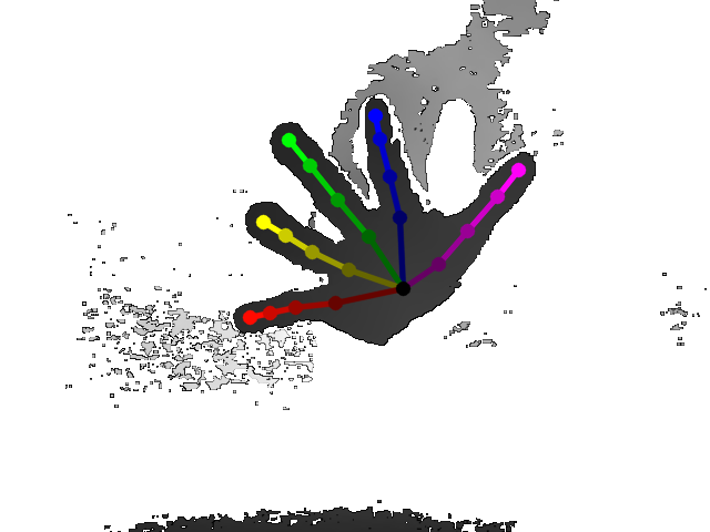
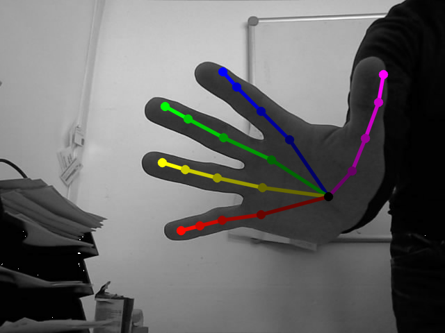
To also evaluate real data, we tested our method on a calibrated camera setup consisting of a depth camera and an RGB camera capturing the hand from two different perspectives. We create 3D annotations using the depth camera and project them into the RGB camera. We can then visually check the projections of the annotations. Fig. 8 shows one example: The joint locations project nearby the real joint locations, which indicates that not only the image coordinates are correct, but also the depth. We refer to the supplemental material for the full sequence.

(a) Depth camera

(b) Projected into RGB camera

Figure 8: Sample frames of our two camera setup. We capture hand articulations from a depth and an RGB camera and apply our method on the depth camera to obtain 3D annotations. These annotations are shown in (a). To evaluate the accuracy, we project the estimated 3D annotations into the RGB camera, which is shown in (b). The full sequence is provided as supplemental material. (Best viewed in color)

4.3 Application to the MSRA Dataset

We applied our approach to the MSRA dataset [24], which is currently the largest dataset for hand pose estimation from single depth images. The authors used a state-of-the-art 3D model-based method [18] to obtain the annotations. As discussed earlier, these annotations are not perfect. We used our method to select $10\%$ of the frames (849 out of 8499 for the first subject) as reference frames and manually provided the 2D locations, visibility, and z-order of the joints for these reference frames. It took on average 45 s per frame for a non-trained annotator to provide this information. We further show a qualitative comparison, and that the higher annotation accuracy leads to better pose estimates, when training a state-of-the-art 3D hand pose estimator [15].

Qualitative Comparison

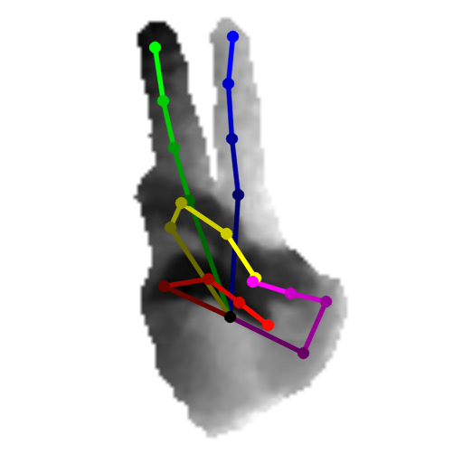
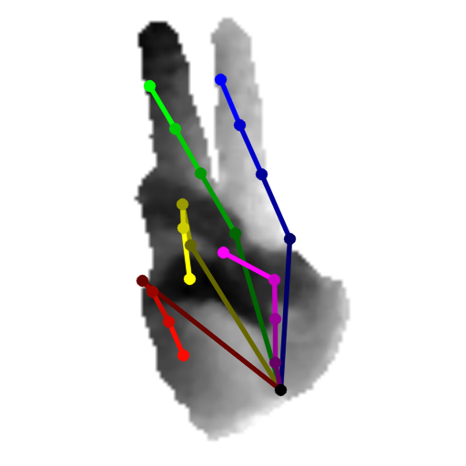
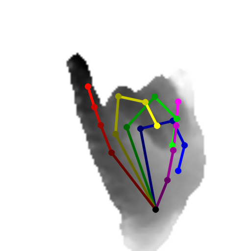
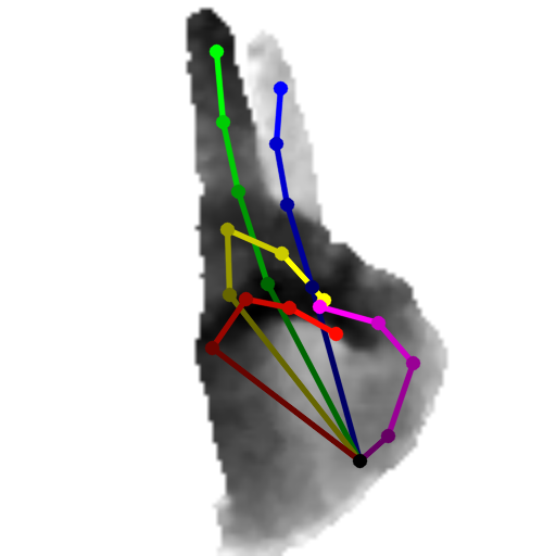
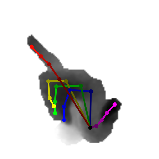
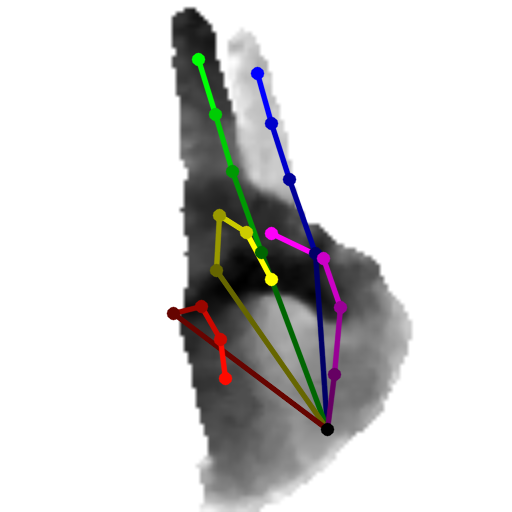
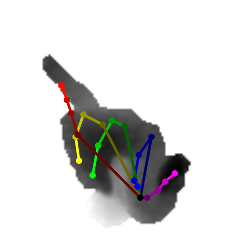
As “real” ground truth is not available, a direct evaluation is not possible. Fig. 9 compares different frames for which the distances between the annotations are large. Our annotations appear systematically better. This strongly suggests that our annotations are more accurate over the sequence. We provide a video sequence that compares the two annotations as a supplemental material.

(a) Frame 970

(b) Frame 1635

(c) Frame 3626

(d) Frame 8495

Figure 9: Qualitative comparison of the annotations obtained using our method (left image) and the annotations of [24] (right image) on the MSRA dataset. We selected several frames with large differences between the two annotations. Note that the shown sample frames are not manually annotated reference frames. (Best viewed in color)

Higher Annotation Accuracy Leads to Better Pose Estimators

We further show that better annotations improve the accuracy of state-of-the-art 3D hand pose estimation methods. We train the method of [15] with the original annotations and compare it with the estimator trained using the annotations we obtained with our method. For the evaluation, we perform 10-fold cross validation, because no explicit test set is specified [24]. The results of this experiment are shown in Fig. 10. The estimator trained with our annotations converges faster, but to similar average joint errors in the end. This indicates that training is easier when the annotations are better. Otherwise, the estimator may focus on difficult, possibly wrongly annotated samples. The results clearly show that accurate training data is necessary to perform accurate inference. The estimator achieves test set errors of $5.58\pm 0.56$ mm using our annotations for training and testing, and $6.41\pm 2.05$ mm using the provided annotations. When we train the pose estimator on the provided annotations but evaluate it on our own annotations, the error is $13.23\pm 6.98$ mm, which indicates discrepancy among the annotations. However, the visual comparison — which is the best that can be done on real data — shows that our annotations are more accurate.

Our anno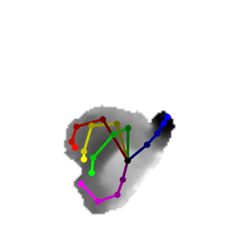
Anno of [24]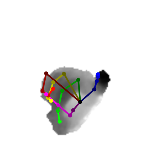
	(a)	(b)	(c)

Figure 10: Training and testing a 3D hand pose estimator with different annotations for the MSRA dataset. We train a state-of-the-art 3D hand pose estimator [15] with the provided annotations and with our revised annotations. We then compare the predicted annotations on a test set. The predictions with our annotations are on the left side. It shows that the estimator learns the incorrect annotations, which leads to inaccurate locations for the test samples. Using our more accurate annotations leads to more accurate results. In (a) note the annotation of the thumb, in (b) the annotations of the pinky and ring fingers, and in (c) the articulation of the index finger. (Best viewed on screen)

4.4 New Egocentric Dataset

Egocentric 3D hand pose estimation is an appealing feature for different Augmented Reality or human computer interaction applications. Creating datasets for this task is very difficult [20]. Egocentric views show severe self-occlusions as fingers are often occluded by the hand and egocentric cameras have a limited field-of-view. Both facts result in a less reliable tracking. Even with manual initialization, fingers are frequently occluded and the hand can move outside the camera view frustum.

We provide a new dataset consisting of more than 2000 frames of several egocentric sequences, each starting and ending with a neutral hand pose and showing a user performing a single or various hand articulations per sequence. We annotated the dataset using our method. In contrast, the 3D model-based implementation of [28] often failed by converging to different local minima, and thus resulted in time consuming fiddling with the model parameters.

We establish a baseline on this dataset, by running two state-of-the-art methods: (1) the method of Oberweger et al. [15], which was shown to be among the best methods for third person hand pose estimation [25], and (2) the method of Supančič et al. [25], which was initially proposed for hand pose estimation, but especially for hand object interaction in egocentric views. We perform 5-fold cross-validation and report the average and standard deviation over the different folds. We report the results in Table 3. The method of Supančič has larger errors, mostly due to flipping ambiguities. For the oracle, we assume the 3D poses known, and return the pose with the smallest Euclidean distance from the training set.

Method	Avg. / median error
Oberweger et al. [15]	$24.58\pm 16.08$ / 19.53 mm
Supančič et al. [25]	$33.09\pm 21.66$ / 26.20 mm
Oracle	$20.20\pm 10.92$ / 19.47 mm

Table 3: Average accuracy on the egocentric hand dataset with 5-fold cross validations. We apply two state-of-the-art methods to the dataset and report the Euclidean 3D joint errors. For the orcle, we calculate the distance to the nearest sample in the training set.

5 Conclusion

Given the recent developments in Deep Learning, the creation of training data may now be the main bottleneck in practical applications of Machine Learning for hand pose estimation. Our method brings a much needed solution to the creation of accurate 3D annotations of hand poses. It avoids the need for motion capture systems, which are cumbersome and cannot always be used, and does not require complex camera setups. Moreover, it could also be applied to any other articulated structures, such as human bodies.

Acknowledgements:

This work was funded by the Christian Doppler Laboratory for Handheld Augmented Reality and the Graz University of Technology FutureLabs fund.

References

- [1] K. Ali, D. Hasler, and F. Fleuret. Flowboost – Appearance Learning from Sparsely Annotated Data. In CVPR, 2011.
- [2] L. Ballan, A. Taneja, J. Gall, L. Van Gool, and M. Pollefeys. Motion Capture of Hands in Action Using Discriminative Salient Points. In ECCV, 2012.
- [3] V. Belagiannis, C. Rupprecht, G. Carneiro, and N. Navab. Robust Optimization for Deep Regression. In ICCV, 2015.
- [4] M. Berkelaar, K. Eikland, and P. Notebaert. Open Source (Mixed-Integer) Linear Programming System, 2005.
- [5] N. Dalal and B. Triggs. Histograms of Oriented Gradients for Human Detection. In CVPR, 2005.
- [6] S. Hinterstoisser, S. Holzer, C. Cagniart, S. Ilic, K. Konolige, N. Navab, and V. Lepetit. Multimodal Templates for Real-Time Detection of Texture-Less Objects in Heavily Cluttered Scenes. In ICCV, 2011.
- [7] C. Ionescu, D. Papava, V. Olaru, and C. Sminchisescu. Human3.6m: Large Scale Datasets and Predictive Methods for 3D Human Sensing in Natural Environments. PAMI, 2014.
- [8] D. Kraft. A Software Package for Sequential Quadratic Programming. Technical report, German Aerospace Center, 1988.
- [9] D. Kuettel, M. Guillaumin, and V. Ferrari. Segmentation Propagation in ImageNet. In ECCV, 2012.
- [10] V. Lepetit and M. Berger. A Semi-Automatic Method for Resolving Occlusions in Augmented Reality. In CVPR, 2000.
- [11] C. Liu, J. Yuen, and A. Torralba. SIFT Flow: Dense Correspondence Across Scenes and Its Applications. PAMI, 33(5), 2011.
- [12] J. Masci, U. Meier, D. Cireşan, and J. Schmidhuber. Stacked Convolutional Auto-Encoders for Hierarchical Feature Extraction. In Proc. of ICANN, 2001.
- [13] S. Melax, L. Keselman, and S. Orsten. Dynamics Based 3D Skeletal Hand Tracking. In Proc. of Graphics Interface Conference, 2013.
- [14] G. L. Nemhauser, L. A. Wolsey, and M. L. Fisher. An Analysis of Approximations for Maximizing Submodular Set Functions - I. Mathematical Programming, 14(1), 1978.
- [15] M. Oberweger, P. Wohlhart, and V. Lepetit. Hands Deep in Deep Learning for Hand Pose Estimation. In Proc. of CVWW, 2015.
- [16] M. Oberweger, P. Wohlhart, and V. Lepetit. Training a Feedback Loop for Hand Pose Estimation. In ICCV, 2015.
- [17] G. Pons-Moll, D. J. Fleet, and B. Rosenhahn. Posebits for Monocular Human Pose Estimation. In CVPR, 2014.
- [18] C. Qian, X. Sun, Y. Wei, X. Tang, and J. Sun. Realtime and Robust Hand Tracking from Depth. In CVPR, 2014.
- [19] G. Riegler, D. Ferstl, M. Rüther, and H. Bischof. A Framework for Articulated Hand Pose Estimation and Evaluation. In Proc. of SCIA, 2015.
- [20] G. Rogez, M. Khademi, J. S. Supancic, J. Montiel, and D. Ramanan. 3D Hand Pose Detection in Egocentric RGB-D Images. In ECCV, 2014.
- [21] G. Rogez, J. S. Supancic, and D. Ramanan. Understanding Everyday Hands in Action from RGB-D Images. In ICCV, 2015.
- [22] C. Sminchisescu and B. Triggs. Kinematic Jump Processes for Monocular 3D Human Tracking. In CVPR, 2003.
- [23] S. Sridhar, A. Oulasvirta, and C. Theobalt. Interactive Markerless Articulated Hand Motion Tracking Using RGB and Depth Data. In ICCV, 2013.
- [24] X. Sun, Y. Wei, S. Liang, X. Tang, and J. Sun. Cascaded Hand Pose Regression. In CVPR, 2015.
- [25] J. S. Supancic, G. Rogez, Y. Yang, J. Shotton, and D. Ramanan. Depth-Based Hand Pose Estimation: Data, Methods, and Challenges. In ICCV, 2015.
- [26] D. Tang, H. J. Chang, A. Tejani, and T.-K. Kim. Latent Regression Forest: Structured Estimation of 3D Articulated Hand Posture. In CVPR, 2014.
- [27] C. J. Taylor. Reconstruction of Articulated Objects from Point Correspondences in a Single Uncalibrated Image. In CVPR, 2000.
- [28] J. Tompson, M. Stein, Y. LeCun, and K. Perlin. Real-Time Continuous Pose Recovery of Human Hands Using Convolutional Networks. ACM Transactions on Graphics, 33, 2014.
- [29] D. Tzionas and J. Gall. A Comparison of Directional Distances for Hand Pose Estimation. In Proc. of GCPR, 2013.
- [30] L. van der Maaten and G. Hinton. Visualizing High-Dimensional Data Using t-SNE. JMLR, 9(Nov), 2008.
- [31] X. Wei and J. Chai. VideoMocap: Modeling Physically Realistic Human Motion from Monocular Video Sequences. ACM Transactions on Graphics, 29(4), 2010.
- [32] A. Wetzler, R. Slossberg, and R. Kimmel. Rule of Thumb: Deep Derotation for Improved Fingertip Detection. In BMVC, 2015.
- [33] Y. Wu, J. Lin, and T. Huang. Capturing Natural Hand Articulation. In ICCV, 2001.
- [34] C. Xu and L. Cheng. Efficient Hand Pose Estimation from a Single Depth Image. In ICCV, 2013.
- [35] H. Yasin, U. Iqbal, B. Krüger, A. Weber, and J. Gall. A Dual-Source Approach for 3D Pose Estimation from a Single Image. In CVPR, 2016.