Discrete symmetries and the Lieb-Schultz-Mattis theorem

Abstract

In this study, we consider one-dimensional (1D) quantum spin systems with translation and discrete symmetries (spin reversal, space inversion and time reversal symmetries). By combining the continuous U(1) symmetry with the discrete symmetries and using the extended Lieb-Schultz-Mattis theorem [1][2], we investigate the relation between the ground states, energy spectra and symmetries. For half-integer spin cases, we generalize the dimer and Néel concepts using the discrete symmetries, and we can reconcile the LSM theorem with the dimer or Néel states, since there was a subtle dilemma. Furthermore, a part of discrete symmetries is enough to classify possible phases. Thus we can deepen our understanding of the relation between the LSM theorem and discrete symmetries.

1 Introduction

In many body quantum systems, it is important to investigate energy spectra, that is, whether gapless or gapped, or the degeneracy of ground states. The structure of energy spectra is related with other physical properties, such as the symmetry breaking. Therefore, in nonrelativistic many body quantum systems, general and rigorous theorems remain important. The Lieb-Schultz-Mattis (LSM) theorem [1] is one of them.

Historically, Lieb, Schultz and Mattis treated the $S=1/2$ XXZ spin chain, and they showed there exists a low energy $O(1/L)$ ($L$: system size) excited state above the ground state. Affleck and Lieb [3] studied general spin $S$ and SU($N$) symmetric cases, and showed the same result as the LSM theorem for half-integer $S$. In addition, they considered the relation between the space inversion and the spin reversal symmetries. Independently, using the twisted boundary condition, Kolb [4] showed, for half-integer spin chains, the nontrivial periodicity of the wave number $q\rightarrow q+\pi$ of the lowest energy dispersion in the zero magnetization subspace. And he discussed the continuity of the energy dispersion for $q$. One limitation of the traditional LSM theorem [1, 3, 5] is the assumption of the unique ground state (or the unique lowest energy state in the fixed magnetization subspace) for the finite system, which is violated in several cases with frustrations (Majumdar-Ghosh model [6, 7] and the incommensurate region). We have separated the proof process of the LSM theorem from the assumption of the unique ground state [2].

In our previous paper, we proved that the lowest energy spectrum is a continuous function of the wave number $q$ for the irrational magnetization, and the nontrivial periodicity of $q$ for the rational magnetization (the latter statement is a generalization of [5]). Here we mean “rational magnetization”, to be the case where the magnetization per site is a relatively simple rational number in the thermodynamic limit:

$$\lim_{L\rightarrow\infty}\frac{S^{z}_{T}}{L}=\frac{m}{n}$$

($L$: system size, $S^{z}_{T}\equiv\sum_{j}S^{z}_{j}$, $m$ and $n$ are coprimes), and “irrational magnetization” otherwise. Thus, there are two possibilities: in the first case, the energy spectrum is continuous with $q$, so it doesn’t have an energy gap (see Fig.1 (a)); secondly, an energy gap exists between the ground state and continuous excited states (see Fig 1 (b)).

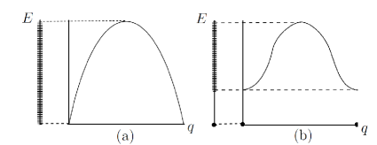
Figure 1: Example of energy spectra:cases (a),(b). Left side bar is side view of spectrum expressing energy distribution.

In a half-integer spin chain with U(1) symmetry at zero magnetization, when the energy spectrum is gapless (case (a)), the low energy modes are at $q=0,\pi$. When the energy spectrum is gapped (case (b)), several possibilities can be considered as the ground states. One candidate is the dimer state:

$$|\Psi_{\rm dimer}\rangle\equiv[1,2][3,4]\dots[L-1,L],\quad[i,i+1]=\frac{1}{\sqrt{2}}(|\uparrow\rangle_{i}|\downarrow\rangle_{i+1}-|\downarrow\rangle_{i}|\uparrow\rangle_{i+1}),$$

and a counterpart produced from the translation by one site. Another one is the Néel state:

$$|\Psi_{\rm N\acute{e}el}\rangle\equiv|\uparrow_{1}\downarrow_{2}\uparrow_{3}\dots\downarrow_{L}\rangle$$

and its counterpart. From these states, we can construct the $q=0,\pi$ wave number states. The $q=0$ states for both cases have a common feature of the discrete symmetries (spin reversal, space inversion and time reversal), whereas at $q=\pi$ the Néel-like state has different discrete symmetries from those of the dimer-like state.

On the other hand, the LSM-type variational state at $q=\pi$ contains both Néel-like (see Eq. (34)) and the dimer-like (see Eq. (33))components. This suggests that both states should be always degenerate with the $q=0$ ground state, which seems unnatural. In fact, in the Majumdar-Ghosh model, only the dimer-like state at $q=\pi$ is degenerate with the $q=0$ ground state [6, 7]. In this study, considering the discrete symmetries, we will show that the normalization is important to resolve this dilemma. Furthermore, we show that a part of the discrete symmetries is enough to distinguish the Néel-like and dimer-like states, and for the normalization discussion. One of the interesting applications is the magnetic plateau [5], to classify the possible phases.

The layout of this paper is as follows. In Sect. 2, we define the symmetries (rotation, space inversion, translation and time reversal) and relating operators, then we discuss the symmetry properties of the Néel or dimer states. Section 3 is a review of the LSM theorem and twisting operators. In Sect. 4, we construct several states with wave number $q=\pi$ by acting the twisting operator to the $q=0$ ground state, then we study the discrete symmetries of the constructed $q=\pi$ states. When U(1) symmetry holds, these $q=\pi$ states have the $O(1/L)$ low energy from the LSM theorem. Section 5 is our main result; we will explain why some of the $q=\pi$ states do not have to satisfy the LSM inequality, considering the normalization of the states. In Sect. 6, we show that a part of discrete symmetries is enough for the above arguments. And we apply our result to several examples ($S=1/2$ NNN XXZ chain, spin ladder, spin tube and distorted diamond chain) in Sect. 7. In Sect. 8, we discuss symmetric properties of the ground state with system sizes $L=4n,4n+2,2n+1$. Section 9 is a summary and discussion.

2 Symmetries and operators

In this section, we explain the symmetries and the operators of the many body system. As an example, we treat a 1D spin system:

$$\hat{H}=\sum_{j=1}^{L}\sum_{r=1}^{L/2}J_{x}(r)\hat{S}^{x}_{j}\hat{S}^{x}_{j+r}+J_{y}(r)\hat{S}^{y}_{j}\hat{S}^{y}_{j+r}+J_{z}(r)\hat{S}^{z}_{j}\hat{S}^{z}_{j+r},$$ (1)

where $(\hat{\bm{S}}_{j})^{2}=S(S+1)$. In addition, the system has a periodic boundary condition ($\hat{S}^{x,y,z}_{L+j}=\hat{S}^{x,y,z}_{j}$) and the system size $L$ is $4n$($n$:integer).

2.1 Rotational operator

We define rotational operators around the $x,y,z$ axes:

$$\hat{U}^{x}_{\theta}\equiv\exp{(-i\theta\hat{S}^{x}_{T})},~{}\hat{S}^{x}_{T}\equiv\sum^{L}_{j=1}\hat{S}^{x}_{j},$$ (2)

$$\hat{U}^{y}_{\theta}\equiv\exp{(-i\theta\hat{S}^{y}_{T})},~{}\hat{S}^{y}_{T}\equiv\sum^{L}_{j=1}\hat{S}^{y}_{j},$$ (3)

$$\hat{U}^{z}_{\theta}\equiv\exp{(-i\theta\hat{S}^{z}_{T})},~{}\hat{S}^{z}_{T}\equiv\sum^{L}_{j=1}\hat{S}^{z}_{j}.$$ (4)

We can calculate, e.g.,

$$(\hat{U}^{x}_{\theta})^{\dagger}\hat{S}^{y}_{k}\hat{U}^{x}_{\theta} =\hat{S}^{y}_{k}+i\theta[\hat{S}_{T}^{x},\hat{S}^{y}_{k}]+\frac{1}{2!}\left(i\theta\right)^{2}[\hat{S}_{T}^{x},[\hat{S}_{T}^{x},\hat{S}^{y}_{k}]]+\cdots$$

$$=\cos{(\theta)}\hat{S}^{y}_{k}-\sin{(\theta)}\hat{S}^{z}_{k}.$$ (5)

2.2 Spin reversal operators

In spin rotational operators, the $\theta=\pi$ case (spin reversal operator) is important. Since $(\hat{U}^{z}_{\pi})^{2}=\exp(-2\pi i\hat{S}_{T}^{z})=1$, the eigenvalue of $\hat{U}^{z}_{\pi}$ is $\pm 1$ (because the eigenvalue of $\hat{S}_{T}^{z}$ is integer for even $L$). In the same way, $(\hat{U}^{x}_{\pi})^{2}=(\hat{U}^{y}_{\pi})^{2}=1$.

2.3 Space inversion operators

We define two kinds of space inversion operators; site inversion (inversion on the lattice site), and link inversion (inversion on the link):

$$\mbox{\ (site inversion)\ }:\hat{P}^{\dagger}_{\rm site}\hat{S}^{x,y,z}_{j}\hat{P}_{\rm site} =\hat{S}^{x,y,z}_{L-j},$$ (6)

$$\mbox{\ (link inversion)\ }:\hat{P}^{\dagger}_{\rm link}\hat{S}^{x,y,z}_{j}\hat{P}_{\rm link} =\hat{S}^{x,y,z}_{L-j+1},$$ (7)

where $\hat{P}^{\dagger}_{\rm site}\hat{S}^{x,y,z}_{L}\hat{P}_{\rm site}=\hat{S}^{x,y,z}_{L}$ and $\hat{P}^{\dagger}_{\rm site}\hat{S}^{x,y,z}_{L/2}\hat{P}_{\rm site}=\hat{S}^{x,y,z}_{L/2}$.

Since $\hat{P}_{\rm site}^{2}=\hat{P}_{\rm link}^{2}=\hat{1}$, the eigenvalues of space inversions are $\pm 1$.

2.4 Translation operator

We define the translation operator by one site as

$$\hat{U}^{\dagger}_{\rm trl}\hat{S}^{x,y,z}_{j}\hat{U}_{\rm trl}=\hat{S}^{x,y,z}_{j+1},$$ (8)

and the wave number $q$ as the eigenvalue of the translation operator:

$$\hat{U}_{\rm trl}|S^{z}_{T};q\rangle=e^{iq}|S^{z}_{T};q\rangle.$$ (9)

The wave number $q$ is periodic as $q\rightarrow q+2\pi$ (Brillouin zone).

2.5 Time reversal operator

We introduce the time reversal operator $\hat{K}$, which has the following properties: for spin operators

$$\hat{K}^{\dagger}\hat{\bm{S}}\hat{K}=-\hat{\bm{S}},$$ (10)

and it is an antilinear operator, i.e., for a complex number $c$

$$\hat{K}^{\dagger}c\hat{K}=c^{*}.$$ (11)

The operator $\hat{K}$ commutes with the rotation, space inversion, and translation operators; however, it does not commute with the twisting operator (see Appendix C).

2.6 Ground state properties

It is natural to assume that at least one of the ground states $|\Psi_{g}\rangle$ has the following symmetry properties:

$$\hat{U}_{\rm trl}|\Psi_{g}\rangle =|\Psi_{g}\rangle,\;\hat{P}_{\rm site}|\Psi_{g}\rangle=\hat{P}_{\rm link}|\Psi_{g}\rangle=|\Psi_{g}\rangle,$$

$$\hat{U}^{y}_{\pi}|\Psi_{g}\rangle =\hat{U}^{z}_{\pi}|\Psi_{g}\rangle=|\Psi_{g}\rangle,\;\hat{K}|\Psi_{g}\rangle=|\Psi_{g}\rangle$$ (12)

(furthermore in the case of U(1) symmetry around the $z$-axis, we assume $\hat{S}^{z}_{T}|\Psi_{g}\rangle=0$). More precisely on the above statement, we consider that there are a finite number of energy eigenstates in a range of $O(1/L)$ above the lowest energy, and the state with symmetry eigenvalues (12) is contained in them.

For nonfrustrated cases, these symmetries (12) for the ground state can be proven by the Marshall-Lieb-Mattis (MLM) theorem with system size $L=4n$ (see Sect. 8). Even in the frustrated case the above statement may remain valid, e.g., one of the ground states of the Majumdar-Ghosh model satisfies (12).

The state $|\Psi_{g}\rangle$ is normalized as $\langle\Psi_{g}|\Psi_{g}\rangle=1$.

2.7 Symmetries and eigenvalues of dimer and Néel states

In this subsection, we consider the symmetry properties of the Néel state or the dimer state. First, we check the symmetry eigenvalues of $q=0$ states

$$|\Psi_{\rm N\acute{e}el1}\rangle+|\Psi_{\rm N\acute{e}el2}\rangle$$ (13)

$$|\Psi_{\rm dimer1}\rangle+|\Psi_{\rm dimer2}\rangle$$ (14)

where

$$|\Psi_{\rm N\acute{e}el1}\rangle\equiv|\uparrow_{1}\downarrow_{2}\uparrow_{3}\dots\downarrow_{L}\rangle,\quad|\Psi_{\rm N\acute{e}el2}\rangle\equiv|\downarrow_{1}\uparrow_{2}\downarrow_{3}\dots\uparrow_{L}\rangle,$$ (15)

and

$$|\Psi_{\rm dimer1}\rangle\equiv[1,2][3,4]\dots[L-1,L],\quad|\Psi_{\rm dimer2}\rangle\equiv[2,3][4,5]\dots[L,1],$$

$$[i,i+1]=\frac{1}{\sqrt{2}}(\uparrow_{i}\downarrow_{i+1}-\downarrow_{i}\uparrow_{i+1}).$$ (16)

Both Eq. (13) and Eq. (14) have $\hat{P}_{\rm site}=1,\hat{P}_{\rm link}=1,\hat{U}^{y}_{\pi}=1,\hat{K}=1$.

On the contrary, the $q=\pi$ states, constructed from the dimer or the Néel states, have different symmetry eigenvalues, so we can distinguish these two states. The Néel-like state

$$|\Psi_{\rm N\acute{e}el-like}\rangle\equiv|\Psi_{\rm N\acute{e}el1}\rangle-|\Psi_{\rm N\acute{e}el2}\rangle$$ (17)

has eigenvalues $q=\pi,\hat{P}_{\rm site}=1,\hat{P}_{\rm link}=-1,\hat{U}^{y}_{\pi}=-1,\hat{K}=-1$. In contrast, dimer-like state

$$|\Psi_{\rm dimer-like}\rangle\equiv|\Psi_{\rm dimer1}\rangle-|\Psi_{\rm dimer2}\rangle$$ (18)

has eigenvalues $q=\pi,\hat{P}_{\rm site}=-1,\hat{P}_{\rm link}=1,\hat{U}^{y}_{\pi}=1,\hat{K}=1$.

In this subsection we have discussed the symmetries of particular cases Eq. (15) and Eq. (16). In the following, we will generalize these symmetry consideration, for wide models, Eq. (1), and quasi 1D spin systems, etc.

3 The LSM theorem

In this section we review the LSM theorem. The assumptions of the LSM theorem are U(1) symmetry, translational symmetry and short-range interaction. For the Hamiltonian (1) it means $J_{x}(r)=J_{y}(r)\propto\exp{(-r/\xi)}$.

In [2] we have proven the following inequality:

$$E(S^{z}_{T},q+\frac{2\pi}{L}S^{z}_{T}+2\pi S)+E(S^{z}_{T},q-\frac{2\pi}{L}S^{z}_{T}+2\pi S)-2E(S^{z}_{T},q)$$

$$\leq\langle S_{T}^{z};q|(\hat{U}_{2\pi}^{tw})^{\dagger}\hat{H}\hat{U}_{2\pi}^{tw}+(\hat{U}_{-2\pi}^{tw})^{\dagger}\hat{H}\hat{U}_{-2\pi}^{tw}-2\hat{H}|S_{T}^{z};q\rangle\leq O(1/L),$$ (19)

where $\hat{U}^{\rm tw}_{2\pi l}$ ($l$: integer) are the twisting operators given by

$$\hat{U}^{\rm tw}_{2\pi l}\equiv\exp\left(-\frac{2\pi il}{L}\sum^{L}_{j=1}j(\hat{S}^{z}_{j}-S)\right),$$ (20)

and $E(S_{T}^{z};q)$ is one of the lowest energies in the $S_{T}^{z};q$ subspace. We introduced the phase factor $\exp(\frac{2\pi il}{L}S\sum_{j=1}^{L}j)$ in Eq. (20), which was absent in the original twisting operator in[1, 3], in order to avoid cumbersome treatments of the edge term $\exp(2\pi il\hat{S}^{z}_{1})$, appearing from the translation operation on the original twisting operator (see also Eq. (115) in Appendix B).

One result of the extended LSM theorem[2] is that if the magnetization is irrational, then the energy spectra must be continuous for $q$. Secondly, by using Eq. (19) and the squeezing technique, we get the next inequality for spin $S$ half-integer:

$$|E(S_{T}^{z}=0;q)-E(S_{T}^{z}=0;q+\pi)|\leq O(1/L).$$ (21)

3.1 Space inversion, spin reversal, and the twisting operator

For the site space inversion, spin reversal and the twisting operator, there are the relations [2, 3]

$$\hat{P}_{\rm site}\hat{U}^{\rm tw}_{2\pi l}=\hat{U}^{\rm tw}_{-2\pi l}\hat{P}_{\rm site},$$ (22)

$$\hat{U}^{y}_{\pi}\hat{U}^{\rm tw}_{2\pi l}=(-1)^{2Sl}\hat{U}^{\rm tw}_{-2\pi l}\hat{U}^{y}_{\pi}.$$ (23)

However, in the link space inversion operation on the twisting operator $\hat{U}^{\rm tw}_{2\pi l}$,

$$\hat{P}_{\rm link}\hat{U}^{\rm tw}_{2\pi l}\hat{P}_{\rm link}=\exp\left(-\frac{2\pi il}{L}\left(\hat{S}^{z}_{T}-SL\right)\right)\hat{U}^{\rm tw}_{-2\pi l},$$ (24)

the prefactor may be confusing with the translation operation on $\hat{U}^{\rm tw}_{2\pi l}$ (see Appendix B). Therefore, we introduce another twisting operator $\hat{U}^{\rm twl}_{2\pi l}$ as [11]

$$\hat{U}^{\rm twl}_{2\pi l}\equiv\exp\left(-\frac{2\pi il}{L}\sum^{L}_{j=1}\left(j-\frac{1}{2}\right)(\hat{S}^{z}_{j}-S)\right),\quad(l:\text{integer})$$ (25)

and then we obtain

$$\hat{P}_{\rm link}\hat{U}^{\rm twl}_{2\pi l}=\hat{U}^{\rm twl}_{-2\pi l}\hat{P}_{\rm link},$$ (26)

$$\hat{U}^{y}_{\pi}\hat{U}^{\rm twl}_{2\pi l}=\hat{U}^{\rm twl}_{-2\pi l}\hat{U}^{y}_{\pi}.$$ (27)

Combining these relations, below two equations are proven[3, 2]:

$$(\hat{P}_{\rm site}\hat{U}^{y}_{\pi})\hat{U}^{\rm tw}_{2\pi l}=(-1)^{2Sl}\hat{U}^{\rm tw}_{2\pi l}(\hat{P}_{\rm site}\hat{U}^{y}_{\pi}),$$ (28)

$$(\hat{P}_{\rm link}\hat{U}^{y}_{\pi})\hat{U}^{\rm twl}_{2\pi l}=\hat{U}^{\rm twl}_{2\pi l}(\hat{P}_{\rm link}\hat{U}^{y}_{\pi}).$$ (29)

Usually, the relation between $\hat{U}^{\rm tw}_{2\pi l}$ and $\hat{U}^{\rm twl}_{2\pi l}$ is not simple, however for the $S^{z}_{T}$=0 case it becomes

$$\hat{U}^{\rm twl}_{2\pi l}|S^{z}_{T}=0\rangle =\exp\left(\frac{\pi il}{L}(\hat{S}^{z}_{T}-SL)\right)\hat{U}^{\rm tw}_{2\pi l}|S^{z}_{T}=0\rangle$$

$$=(-i)^{2Sl}\hat{U}^{\rm tw}_{2\pi l}|S^{z}_{T}=0\rangle.$$ (30)

4 Discrete symmetries and the LSM theorem

4.1 Set of the spin reversal operators’ eigenvalues

We consider the Hamiltonian with spin reversal symmetries ($[\hat{U}^{x}_{\pi},\hat{H}]=[\hat{U}^{y}_{\pi},\hat{H}]=[\hat{U}^{z}_{\pi},\hat{H}]=0$) like Eq. (1). In this case, one can choose a simultaneous eigenstate for the Hamiltonian and spin reversal operators. There is another restriction for the spin reversal operators (see Appendix A):

$$\hat{U}^{x}_{\pi}\hat{U}^{y}_{\pi}\hat{U}^{z}_{\pi}=1.$$ (31)

Therefore, the set of spin reversal eigenvalues should be

$$(\hat{U}^{x}_{\pi},\hat{U}^{y}_{\pi},\hat{U}^{z}_{\pi})=(1,1,1),(-1,-1,1),(-1,1,-1),(1,-1,-1).$$ (32)

In fact, since the spin reversal operators $\hat{U}^{x}_{\pi},\hat{U}^{y}_{\pi},\hat{U}^{z}_{\pi}$ satisfy ($\hat{U}^{x}_{\pi})^{2}=(\hat{U}^{y}_{\pi})^{2}=(\hat{U}^{z}_{\pi})^{2}=\hat{1}$ and Eq. (31), the set {$\hat{1},\hat{U}^{x}_{\pi},\hat{U}^{y}_{\pi},\hat{U}^{z}_{\pi}$} form the Klein four-group, which is isomorphic to the $Z_{2}\times Z_{2}$ group.

4.2 Expression of the states with wave number $q=\pi$ by twisting operators

In this subsection, by using the twisting operators, we construct the spin reversal eigenstates. In the subspace $q=\pi$, we consider the four states

$$\frac{i}{2}(\hat{U}^{\rm tw}_{2\pi}-\hat{U}^{\rm tw}_{-2\pi})|\Psi_{g}\rangle \equiv|\Psi_{\rm DL}\rangle,$$ (33)

$$\frac{1}{2}(\hat{U}^{\rm tw}_{2\pi}+\hat{U}^{\rm tw}_{-2\pi})|\Psi_{g}\rangle \equiv|\Psi_{\rm NL}\rangle,$$ (34)

$$\frac{1}{2}(\hat{U}_{\pi/2}^{x}+\hat{U}_{-\pi/2}^{x})|\Psi_{\rm NL}\rangle \equiv|\Psi_{\rm DB1}\rangle,$$ (35)

$$\frac{1}{2}(\hat{U}_{\pi/2}^{y}+\hat{U}_{-\pi/2}^{y})|\Psi_{\rm NL}\rangle \equiv|\Psi_{\rm DB2}\rangle,$$ (36)

where the phase factors are determined so that the matrix components of the states become real under the $\hat{S}^{z}_{j}$ diagonal representation.

At first, we can calculate the spin reversal eigenvalues of $|\Psi_{\rm DL}\rangle$ as ($1,1,1$) and $|\Psi_{\rm NL}\rangle$ as ($-1,-1,1$), by using Eqs. (23) and (31) and $[\hat{S}_{T}^{z},\hat{U}^{\rm tw}_{2\pi l}]=0$.

Next, using the relation $(\hat{U}_{\pi/2}^{x})^{\dagger}\hat{U}^{y}_{\pi}\hat{U}_{\pi/2}^{x}=(\hat{U}^{z}_{\pi})^{\dagger}=\hat{U}^{z}_{\pi}$ and Eq.(34), we can derive the eigenvalue of $\hat{U}^{y}_{\pi}$ for the state $|\Psi_{\rm DB1}\rangle$ from the calculation

$$\hat{U}^{y}_{\pi}\hat{U}_{\pi/2}^{x}|\Psi_{NL}\rangle=\hat{U}_{\pi/2}^{x}\hat{U}^{z}_{\pi}|\Psi_{NL}\rangle=\hat{U}_{\pi/2}^{x}|\Psi_{NL}\rangle.$$ (37)

Similarly, using the relations $(\hat{U}_{\pi/2}^{x})^{\dagger}\hat{U}^{z}_{\pi}\hat{U}_{\pi/2}^{x}=\hat{U}^{y}_{\pi},(\hat{U}_{\pi/2}^{x})^{\dagger}\hat{U}^{x}_{\pi}\hat{U}_{\pi/2}^{x}=\hat{U}^{x}_{\pi}$, the state $|\Psi_{\rm DB1}\rangle$ has eigenvalues $(\hat{U}^{x}_{\pi},\hat{U}^{y}_{\pi},\hat{U}^{z}_{\pi})=(-1,1,-1)$.

In summary, the four states (33) - (36) have the following eigenvalues:

$$\hat{U}^{x}_{\pi}|\Psi_{\rm DL}\rangle=|\Psi_{\rm DL}\rangle, \hat{U}^{y}_{\pi}|\Psi_{\rm DL}\rangle=|\Psi_{\rm DL}\rangle, \hat{U}^{z}_{\pi}|\Psi_{\rm DL}\rangle=|\Psi_{\rm DL}\rangle,$$ (38)

$$\hat{U}^{x}_{\pi}|\Psi_{\rm NL}\rangle=-|\Psi_{\rm NL}\rangle, \hat{U}^{y}_{\pi}|\Psi_{\rm NL}\rangle=-|\Psi_{\rm NL}\rangle, \hat{U}^{z}_{\pi}|\Psi_{\rm NL}\rangle=|\Psi_{\rm NL}\rangle,$$ (39)

$$\hat{U}^{x}_{\pi}|\Psi_{\rm DB1}\rangle=-|\Psi_{\rm DB1}\rangle, \hat{U}^{y}_{\pi}|\Psi_{\rm DB1}\rangle=|\Psi_{\rm DB1}\rangle, \hat{U}^{z}_{\pi}|\Psi_{\rm DB1}\rangle=-|\Psi_{\rm DB1}\rangle,$$ (40)

$$\hat{U}^{x}_{\pi}|\Psi_{\rm DB2}\rangle=|\Psi_{\rm DB2}\rangle, \hat{U}^{y}_{\pi}|\Psi_{\rm DB2}\rangle=-|\Psi_{\rm DB2}\rangle, \hat{U}^{z}_{\pi}|\Psi_{\rm DB2}\rangle=-|\Psi_{\rm DB2}\rangle.$$ (41)

4.3 Discrete symmetries of the DL and NL states

In this subsection, we discuss the space inversion and time reversal symmetries of these states.

First, we consider $|\Psi_{\rm DL}\rangle$ of Eq. (33). By using Eqs. (22) - (27) and (30), we obtain

$$\hat{P}_{\rm site}|\Psi_{\rm DL}\rangle =-|\Psi_{\rm DL}\rangle,$$ (42)

$$\hat{P}_{\rm link}|\Psi_{\rm DL}\rangle =|\Psi_{\rm DL}\rangle.$$ (43)

For the time reversal symmetry, by using properties (10), (11), and $\hat{U}^{\rm tw}_{2\pi l}\hat{K}=(-1)^{2Sl}\hat{K}\hat{U}^{\rm tw}_{2\pi l}$ (see Appendix C), for half-integer $S$, we obtain

$$\hat{K}|\Psi_{\rm DL}\rangle=|\Psi_{\rm DL}\rangle.$$ (44)

Therefore, $|\Psi_{\rm DL}\rangle$ corresponds to $|\Psi_{\rm dimer-like}\rangle$ of Eq. (18).

Similarly, by using Eqs. (22) - (27) and (30), we show the state $|\Psi_{\rm NL}\rangle$ of Eq. (34) satisfies the relations below in half-integer spin:

$$\hat{P}_{\rm site}|\Psi_{\rm NL}\rangle =|\Psi_{\rm NL}\rangle,$$ (45)

$$\hat{P}_{\rm link}|\Psi_{\rm NL}\rangle =-|\Psi_{\rm NL}\rangle,$$ (46)

$$\hat{K}|\Psi_{\rm NL}\rangle =-|\Psi_{\rm NL}\rangle.$$ (47)

Therefore, $|\Psi_{\rm NL}\rangle$ corresponds to $|\Psi_{\rm N\acute{e}el-like}\rangle$ of Eq.(17).

The rest of the $q=\pi$ states, i.e. $|\Psi_{\rm DB1,DB2}\rangle$, have the symmetries

$$\hat{P}_{\rm site}|\Psi_{\rm DB1,DB2}\rangle=|\Psi_{\rm DB1,DB2}\rangle,$$ (48)

$$\hat{P}_{\rm link}|\Psi_{\rm DB1,DB2}\rangle=-|\Psi_{\rm DB1,DB2}\rangle,$$ (49)

because of $[\hat{P}_{\rm site,link},\hat{U}_{\pi/2}^{x}]=[\hat{P}_{\rm site,link},\hat{U}_{\pi/2}^{y}]=0$.

4.4 The $q=\pi$ states with U(1) symmetry

In the Hamiltonian with U(1) symmetry, the energy expectation for the state (35) is equal to that for (36). Using $(\hat{U}^{z}_{\pi/2})^{\dagger}\hat{H}\hat{U}^{z}_{\pi/2}=\hat{H}$ and the relationship $\hat{U}^{z}_{\pi/2}\hat{U}^{x}_{\pi/2}(\hat{U}^{z}_{\pi/2})^{\dagger}=\hat{U}^{y}_{\pi/2},$ we show

$$\langle\Psi_{\rm DB1}|\hat{H}|\Psi_{\rm DB1}\rangle =\langle\Psi_{\rm NL}|(\hat{U}_{\pi/2}^{x})^{\dagger}\hat{H}\hat{U}_{\pi/2}^{x}|\Psi_{\rm NL}\rangle$$

$$=\langle\Psi_{\rm NL}|(\hat{U}_{\pi/2}^{x})^{\dagger}(\hat{U}^{z}_{\pi/2})^{\dagger}\hat{H}\hat{U}^{z}_{\pi/2}\hat{U}_{\pi/2}^{x}|\Psi_{\rm NL}\rangle$$

$$=\langle\Psi_{\rm NL}|(\hat{U}_{\pi/2}^{y})^{\dagger}\hat{H}\hat{U}_{\pi/2}^{y}|\Psi_{\rm NL}\rangle$$

$$=\langle\Psi_{\rm DB2}|\hat{H}|\Psi_{\rm DB2}\rangle.$$ (50)

Secondly, Eq. (40) ($\hat{U}^{z}_{\pi}|\Psi_{\rm DB1}\rangle=-|\Psi_{\rm DB1}\rangle$) means that the components $S^{z}_{T}\neq 0$ (more strictly $S^{z}_{T}$ odd) should be contained in the state $|\Psi_{\rm DB1}\rangle$. The same statement is valid for $|\Psi_{\rm DB2}\rangle$. Therefore, from the extended LSM theorem [2], these two states must be part of the continuous energy spectra for the wave number $q$.

On the other hand, states (38) and (39) have the eigenvalue $\hat{S}^{z}_{T}=0$, and therefore they may have an energy gap. Note that to satisfy Eq. (21), at least one of the dimer-like state $|\Psi_{\rm DL}\rangle$ and the Néel-like state $|\Psi_{\rm NL}\rangle$ must be degenerate with the ground states ( for more details, see Sect. 5).

4.5 The ground state with SU(2) symmetry

In the case of SU(2) symmetry, we can classify the four cases (32) as

 singlet $$: (\hat{U}^{x}_{\pi},\hat{U}^{y}_{\pi},\hat{U}^{z}_{\pi})=(1,1,1)$$ (51)

 triplet $$: (\hat{U}^{x}_{\pi},\hat{U}^{y}_{\pi},\hat{U}^{z}_{\pi})=(-1,-1,1),(-1,1,-1),(1,-1,-1)$$ (52)

where the triplet states are degenerate in energy. This can be proven by using a similar argument to Eq. (50).

It is proven that the triplet state has a continuous energy spectrum versus wave number by using extended LSM theorem. It means that only the $(\hat{U}^{x}_{\pi},\hat{U}^{y}_{\pi},\hat{U}^{z}_{\pi})=(1,1,1)$ state can have an energy gap.

In summary, there are two possibilities for energy spectra for the SU(2) symmetric case. One is that the energy spectrum is gapless. The other is that the energy gap exists between the dimer-like ground states and the continuous energy spectra (i.e., the ground states are degenerate at $q=0,\pi$, and the $q=\pi$ state must satisfy the relations (38), (42), (43), and (44)).

5 Normalization of the DL and NL states

As we have discussed in the previous section, the dimer-like state (33) and Néel-like state (34) are expressed by twisting operators. By the way, the states $\hat{U}^{\rm tw}_{\pm 2\pi}|\Psi_{g}\rangle$ have wave number $q=\pi$, and the energy expectation value of them is degenerate with the ground state in $O(1/L)$ because of the LSM theorem. So, one may think that both the dimer-like and the Néel-like states should be always degenerate with the $q=0$ ground state. However it seems unnatural. The answer to this paradox is in the normalization of the states. In fact, the dimer-like and Néel-like states are not normalized, although the component operator is unitary. If the expectation of one of the states is zero in the infinite limit ($L\rightarrow\infty$), it may have an energy gap without breaking the inequality of the LSM theorem.

	$N_{\rm DL}$	$N_{\rm NL}$	$G_{\rm DL}$	$G_{\rm NL}$
case1	Finite	Finite	0	0
case2	1	0	0	May be gapped
case3	0	1	May be gapped	0

Table 1: Possible relations of the dimer-like energy $G_{\rm DL}$ (55) and the Néel-like energy $G_{\rm NL}$ (56), and norms for dimer-like $N_{\rm DL}$ (53) and Néel-like $N_{\rm NL}$ (54), in the infinite limit ($L\rightarrow\infty$).

We classify these possibilities as in Table 1, where $N_{\rm DL},N_{\rm NL}$ are given by

$$N_{\rm DL}\equiv\langle\Psi_{\rm DL}|\Psi_{\rm DL}\rangle\geq 0,$$ (53)

$$N_{\rm NL}\equiv\langle\Psi_{\rm NL}|\Psi_{\rm NL}\rangle\geq 0,$$ (54)

and $G_{\rm DL}$ and $G_{\rm NL}$ are defined as

$$G_{\rm DL}\equiv N_{\rm DL}^{-1}\langle\Psi_{\rm DL}|\hat{H}|\Psi_{\rm DL}\rangle-\langle\Psi_{g}|\hat{H}|\Psi_{g}\rangle,$$ (55)

$$G_{\rm NL}\equiv N_{\rm NL}^{-1}\langle\Psi_{\rm NL}|\hat{H}|\Psi_{\rm NL}\rangle-\langle\Psi_{g}|\hat{H}|\Psi_{g}\rangle.$$ (56)

Then $|\Psi_{\rm DL}\rangle$ and $|\Psi_{\rm NL}\rangle$ are candidates of the ground state with $q=\pi$. We can distinguish these two states as

$$\hat{P}_{\rm site}|\Psi_{\rm DL}\rangle =-|\Psi_{\rm DL}\rangle, \hat{P}_{\rm link}|\Psi_{\rm DL}\rangle =|\Psi_{\rm DL}\rangle, \hat{U}^{y}_{\pi}|\Psi_{\rm DL}\rangle =|\Psi_{\rm DL}\rangle,$$ (57)

$$\hat{P}_{\rm site}|\Psi_{\rm NL}\rangle =|\Psi_{\rm NL}\rangle, \hat{P}_{\rm link}|\Psi_{\rm NL}\rangle =-|\Psi_{\rm NL}\rangle, \hat{U}^{y}_{\pi}|\Psi_{\rm NL}\rangle =-|\Psi_{\rm NL}\rangle.$$ (58)

Now, we will explain the reason for the classification in Table 1. Using Eqs. (33) and (34), we obtain

$$|\Psi_{\rm NL}\rangle-i|\Psi_{\rm DL}\rangle=\hat{U}^{\rm tw}_{2\pi}|\Psi_{g}\rangle,$$ (59)

where the right-hand side of Eq. (59) is normalized ($\langle\Psi_{g}|(\hat{U}^{\rm tw}_{2\pi})^{\dagger}\hat{U}^{\rm tw}_{2\pi}|\Psi_{g}\rangle=1$). Since $\hat{U}_{\pi}^{y}|\Psi_{\rm DL}\rangle=|\Psi_{\rm DL}\rangle$ and $\hat{U}_{\pi}^{y}|\Psi_{\rm NL}\rangle=-|\Psi_{\rm NL}\rangle$, the next relation is derived:

$$\langle\Psi_{\rm DL}|\Psi_{\rm NL}\rangle=\langle\Psi_{\rm DL}|\hat{U}_{\pi}^{y}|\Psi_{\rm NL}\rangle=-\langle\Psi_{\rm DL}|\Psi_{\rm NL}\rangle=0.$$ (60)

Therefore the norm of the left-hand side of Eq. (59) is

$$(\langle\Psi_{\rm NL}|+i\langle\Psi_{\rm DL}|)(|\Psi_{\rm NL}\rangle-i|\Psi_{\rm DL}\rangle)=N_{\rm DL}+N_{\rm NL}=1.$$ (61)

Next, because of extended LSM theorem [2], next inequality is satisfied:

$$|\langle\Psi_{g}|(\hat{U}_{2\pi}^{\rm tw})^{\dagger}\hat{H}\hat{U}_{2\pi}^{\rm tw}-\hat{H}|\Psi_{g}\rangle|\leq O(1/L).$$ (62)

Since

$$\langle\Psi_{\rm NL}|\hat{H}|\Psi_{\rm DL}\rangle=0,$$ (63)

we obtain

$$\langle\Psi_{g}|(\hat{U}_{2\pi}^{\rm tw})^{\dagger}\hat{H}\hat{U}_{2\pi}^{\rm tw}|\Psi_{g}\rangle=\langle\Psi_{\rm NL}|\hat{H}|\Psi_{\rm NL}\rangle+\langle\Psi_{\rm DL}|\hat{H}|\Psi_{\rm DL}\rangle.$$ (64)

By using Eq. (55)$\times N_{\rm DL}+$ Eq.(56)$\times N_{\rm NL}$, Eqs. (61) and (64), then Eq. (62) is expressed as

$$|N_{\rm DL}G_{\rm DL}+N_{\rm NL}G_{\rm NL}|\leq O(1/L).$$ (65)

By Eq. (65), we can prove Table 1.

Finally, in this section we have used the symmetric property of the Hamiltonian only at Eqs. (62) and (63). For Eq. (62), the U(1) and the translation symmetries of the Hamiltonian are required. For Eq. (63), the discrete symmetries are required.

6 Partial discrete symmetry

In the previous sections, in addition to the translational and U(1) symmetries, we have assumed the full discrete symmetries, i.e., spin reversal and space inversion and time reversal symmetries. However, as we will discuss in this section, with a part of the discrete symmetries (spin reversal or space inversion or time reversal), some of the results, including Table 1 in Sect. 5, hold.

6.1 Spin reversal symmetry only

We consider the interaction with spin reversal symmetry, whereas space inversion symmetry and time reversal symmetry are broken: $[\hat{H},\hat{U}^{y}_{\pi}]=0$ but $[\hat{H},\hat{P}]\neq 0,[\hat{H},\hat{K}]\neq 0$. An example is

$$\hat{H}_{DM}=\sum_{j}\bm{S}_{j}\cdot(\bm{S}_{j+1}\times\bm{S}_{j+2}).$$ (66)

In this case, one of the ground states should have the properties

$$\hat{U}^{y}_{\pi}|\Psi_{g}\rangle=\hat{U}^{z}_{\pi}|\Psi_{g}\rangle=|\Psi_{g}\rangle,\hat{S}^{z}_{T}|\Psi_{g}\rangle=0,$$ (67)

whereas $\hat{P}|\Psi_{g}\rangle$ and $\hat{K}|\Psi_{g}\rangle$ are not well defined. Although there is the possibility of a nonzero wave number $q\neq 0$ ground state, the wave number of $|\Psi_{\rm DL}\rangle$ or $|\Psi_{\rm NL}\rangle$ is different from that of the $|\Psi_{g}\rangle$, and therefore $\langle\Psi_{\rm DL}|\Psi_{g}\rangle=\langle\Psi_{\rm NL}|\Psi_{g}\rangle=0$.

Using the spin reversal symmetry, one can distinguish the dimer-like state $|\Psi_{\rm DL}\rangle$ and the Néel-like state $|\Psi_{\rm NL}\rangle$:

$$\hat{U}^{y}_{\pi}|\Psi_{\rm DL}\rangle=|\Psi_{\rm DL}\rangle,\quad\hat{U}^{y}_{\pi}|\Psi_{\rm NL}\rangle=-|\Psi_{\rm NL}\rangle.$$ (68)

Since $[\hat{H},\hat{U}^{y}_{\pi}]=0$, we show

$$\langle\Psi_{\rm NL}|\hat{H}|\Psi_{\rm DL}\rangle=0.$$ (69)

Therefore, we can obtain the same result as Table 1.

6.2 Space inversion symmetry only

Next we consider the case with space inversion symmetry, whereas the spin reversal symmetry and time reversal symmetry are broken, i.e., $[\hat{H},\hat{P}]=0$ but $[\hat{H},\hat{U}^{y}_{\pi}]\neq 0,[\hat{H},\hat{K}]\neq 0$.

In this case, one of the ground states should have the properties

$$\hat{U}_{\rm trl}|\Psi_{g}\rangle=|\Psi_{g}\rangle,$$ (70)

whereas $\hat{U}^{y}_{\pi}|\Psi_{g}\rangle$ and $\hat{K}|\Psi_{g}\rangle$ are not well defined, which means the possibility of a nonzero magnetization. About space inversions, we assume either

$$\hat{P}_{\rm site}|\Psi_{g}\rangle=|\Psi_{g}\rangle$$ (71)

or

$$\hat{P}_{\rm link}|\Psi_{g}\rangle=|\Psi_{g}\rangle.$$ (72)

In Sect. 5, we saw that the $q=0,\pi$ wave number states are important, thus we consider the following rational magnetization cases:

$$\hat{S}^{z}_{T}|\Psi_{g}\rangle=\left(S-\frac{m}{2n}\right)L|\Psi_{g}\rangle$$ (73)

($m,n$ are integers such that $m$ and $2n$ are coprime, independent of $L$), where the lowest spectrum has $q\rightarrow q+\pi/n$ nontrivial periodicity:

$$|E(S^{z}_{T};q)-E(S^{z}_{T};q+\pi/n)|\leq O(1/L).$$ (74)

In this case, from the next relation (see Appendix B),

$$\hat{U}_{\rm trl}\hat{U}^{\rm tw}_{\pm 2\pi n}|\Psi_{g}\rangle=-\hat{U}^{\rm tw}_{\pm 2\pi n}|\Psi_{g}\rangle,$$ (75)

the states $\hat{U}^{\rm tw}_{\pm 2\pi n}|\Psi_{g}\rangle$ have wave number $q=\pi$. Note that the system size $L$ must satisfy the condition that $L/(2n)$ is integer.

6.2.1 Site space inversion symmetry

In the $[\hat{H},\hat{P}_{\rm site}]=0$ case, we should redefine states (33) and (34) as

$$\frac{i}{2}(\hat{U}^{\rm tw}_{2\pi n}-\hat{U}^{\rm tw}_{-2\pi n})|\Psi_{g}\rangle\equiv|\Psi_{\rm DL^{\prime}}\rangle,$$ (76)

$$\frac{1}{2}(\hat{U}^{\rm tw}_{2\pi n}+\hat{U}^{\rm tw}_{-2\pi n})|\Psi_{g}\rangle\equiv|\Psi_{\rm NL^{\prime}}\rangle.$$ (77)

Using the site space inversion symmetry, one can distinguish the dimer-like state $|\Psi_{\rm DL^{\prime}}\rangle$ and the Néel-like state $|\Psi_{\rm NL^{\prime}}\rangle$:

$$\hat{P}_{\rm site}|\Psi_{\rm DL^{\prime}}\rangle=-|\Psi_{\rm DL^{\prime}}\rangle,\quad\hat{P}_{\rm site}|\Psi_{\rm NL^{\prime}}\rangle=|\Psi_{\rm NL^{\prime}}\rangle.$$ (78)

Since $[\hat{H},\hat{P}_{\rm site}]=0$, we show

$$\langle\Psi_{\rm NL^{\prime}}|\hat{H}|\Psi_{\rm DL^{\prime}}\rangle=0.$$ (79)

Therefore, we can obtain the same result as Table 1.

6.2.2 Link space inversion symmetry

In the $[\hat{H},\hat{P}_{\rm link}]=0$ case, we should redefine states (33) and (34) as

$$\frac{1}{2}(\hat{U}^{\rm twl}_{2\pi n}+\hat{U}^{\rm twl}_{-2\pi n})|\Psi_{g}\rangle\equiv|\Psi_{\rm DL^{\prime\prime}}\rangle,$$ (80)

$$\frac{i}{2}(\hat{U}^{\rm twl}_{2\pi n}-\hat{U}^{\rm twl}_{-2\pi n})|\Psi_{g}\rangle\equiv|\Psi_{\rm NL^{\prime\prime}}\rangle.$$ (81)

Using the link space inversion symmetry, one can distinguish the dimer-like state $|\Psi_{\rm DL^{\prime\prime}}\rangle$ and the Néel-like state $|\Psi_{\rm NL^{\prime\prime}}\rangle$:

$$\hat{P}_{\rm link}|\Psi_{\rm DL^{\prime\prime}}\rangle=|\Psi_{\rm DL^{\prime\prime}}\rangle,\quad\hat{P}_{\rm link}|\Psi_{\rm NL^{\prime\prime}}\rangle=-|\Psi_{\rm NL^{\prime\prime}}\rangle.$$ (82)

Since $[\hat{H},\hat{P}_{\rm link}]=0$, we show

$$\langle\Psi_{\rm NL^{\prime\prime}}|\hat{H}|\Psi_{\rm DL^{\prime\prime}}\rangle=0.$$ (83)

Therefore, we can obtain the same result as Table 1.

Note that when there is spin reversal or time reversal symmetry, Eqs. (80) and (81) satisfy

$$\hat{U}^{y}_{\pi}|\Psi_{\rm DL^{\prime\prime}}\rangle=|\Psi_{\rm DL^{\prime\prime}}\rangle,\quad\hat{U}^{y}_{\pi}|\Psi_{\rm NL^{\prime\prime}}\rangle=-|\Psi_{\rm NL^{\prime\prime}}\rangle$$ (84)

or

$$\hat{K}|\Psi_{\rm DL^{\prime\prime}}\rangle=|\Psi_{\rm DL^{\prime\prime}}\rangle,\quad\hat{K}|\Psi_{\rm NL^{\prime\prime}}\rangle=-|\Psi_{\rm NL^{\prime\prime}}\rangle.$$ (85)

6.3 Time reversal symmetry only

Finally we consider the interaction with time reversal symmetry, whereas the space inversion symmetry and spin reversal symmetry are broken: $[\hat{H},\hat{K}]=0$ but $[\hat{H},\hat{P}]\neq 0,[\hat{H},\hat{U}^{y}_{\pi}]\neq 0$. An example is

$$\hat{H}_{DM}=\sum_{j}(\bm{S}_{j}\times\bm{S}_{j+1})^{z}.$$ (86)

In this case, one of the ground states should have the properties

$$\hat{K}|\Psi_{g}\rangle=|\Psi_{g}\rangle,\hat{S}^{z}_{T}|\Psi_{g}\rangle=0,$$ (87)

whereas $\hat{P}|\Psi_{g}\rangle$ and $\hat{U}^{y}_{\pi}|\Psi_{g}\rangle$ are not well defined. Although there is a possibility of the $q\neq 0$ ground state, the wave number of $|\Psi_{\rm DL}\rangle$ or $|\Psi_{\rm NL}\rangle$ is different from that of the $|\Psi_{g}\rangle$, and therefore $\langle\Psi_{\rm DL}|\Psi_{g}\rangle=\langle\Psi_{\rm NL}|\Psi_{g}\rangle=0$.

Using the time reversal symmetry, one can distinguish the dimer-like state $|\Psi_{\rm DL}\rangle$ and the Néel-like state $|\Psi_{\rm NL}\rangle$ as

$$\hat{K}|\Psi_{\rm DL}\rangle=|\Psi_{\rm DL}\rangle,\quad\hat{K}|\Psi_{\rm NL}\rangle=-|\Psi_{\rm NL}\rangle.$$ (88)

Since $[\hat{H},\hat{K}]=0$, we show

$$\langle\Psi_{\rm NL}|\hat{H}|\Psi_{\rm DL}\rangle=0.$$ (89)

Therefore, we can obtain the same result as Table 1.

7 Examples

Since we have used symmetries except short-range interaction, we can apply our consideration for various models.

7.1 $S=1/2$ spin chain with next-nearest-neighbor interaction

7.1.1 XXZ case

We consider the $S=1/2$ XXZ spin chain with nearest- and next-nearest-neighbor (NNN) interactions:

$$H=J_{1}\left(\sum_{j}\hat{S}^{x}_{j}\hat{S}^{x}_{j+1}+\hat{S}^{y}_{j}\hat{S}^{y}_{j+1}+\Delta\hat{S}^{z}_{j}\hat{S}^{z}_{j+1}\right)+J_{2}\left(\sum_{j}\hat{S}^{x}_{j}\hat{S}^{x}_{j+2}+\hat{S}^{y}_{j}\hat{S}^{y}_{j+2}+\Delta\hat{S}^{z}_{j}\hat{S}^{z}_{j+2}\right)$$ (90)

At $J_{2}=0$, there is an exact solution by Bethe Ansatz, where $\Delta\leq 1$ gapless, and $\Delta>1$ is the gapped Néel ordered phase. At $J_{2}/J_{1}=1/2$, this model was solved by [6, 7] and [8], and it is known that the model has the twofold degenerate dimer ground states as Eq. (16).

In the region ($J_{1}>0,\>J_{2}/J_{1}\leq 1/2,\>\Delta>0$) [9, 10] there are three phases: the Néel, dimer and spin-fluid (XY) phases. The Néel phase corresponds to case 3 of Table 1 in Sect. 5, the dimer phase corresponds to case 2, and finally the spin-fluid phase corresponds to case 1 (where the doublet states ($S^{z}_{T}=\pm 1,q=\pi,\hat{P}_{\rm site}=1,\hat{P}_{\rm link}=-1$) are the lowest energy excitation). The Néel and dimer phases are gapped, whereas the spin-fluid phase is gapless.

About the phase boundary, between the Néel phase and the dimer phase there is a second-order transition line (Gaussian line). The Gaussian line is characterized by the energy level crossing of the Néel-like state ($S^{z}_{T}=0,q=\pi,\hat{U}^{y}_{\pi}=-1,\hat{P}_{\rm site}=1,\hat{P}_{\rm link}=-1,\hat{K}=-1$) and the dimer-like state ($S^{z}_{T}=0,q=\pi,\hat{U}^{y}_{\pi}=1,\hat{P}_{\rm site}=-1,\hat{P}_{\rm link}=1,\hat{K}=1$).

The phase boundary between the spin-fluid phase and the Néel phase, which lies on the $\Delta=1,J_{2}/J_{1}\leq 0.2411$, and the phase boundary between the spin-fluid and the dimer phases, are of the Berezinskii-Kosterlitz-Thouless (BKT) type. The BKT phase boundaries are determined by the energy level crossing of the doublet states and the Néel-like state, or the doublet states and the dimer-like state (the level spectroscopy method, see [10] and [11] ). The BKT multicritical point at $\Delta=1,J_{2}/J_{1}=0.2411$ [12] is determined by the energy level crossing of the triplet (the doublet states and the Néel-like state ) and the dimer-like state. In summary, the consideration on symmetries in this work gives another support for the level spectroscopy, besides the field theory and the renormalization.

In the region ($J_{1}>0,\>J_{2}/J_{1}>1/2,\>\Delta>1$) [13], there are the dimer phase and the (2,2) antiphase (or up-up-down-down) state phase. In the latter phase, there are the four ground states $q=0,\pm\pi/2,\pi$, and above them there is an energy gap. The phase transition between the dimer and the (2,2) antiphase state phase is considered of the 2D Ising universality class.

7.1.2 Isotropic case

Next we consider the isotropic NNN chain, i.e., $\Delta=1$ in Eq. (90).

In the region $J_{1}<0,\>J_{2}/|J_{1}|\leq 1/4$, there is a ferromagnetic phase.

In the region $J_{1}>0,\>J_{2}/J_{1}\leq 0.2411$ [12], this model is gapless at the wave number $q=0,\pi$, and the universality class is of a Tomonaga-Luttinger type. In the region $J_{1}>0,\>J_{2}/J_{1}>0.2411$, there is a gapped phase with the dimer-long range order.

At $J_{1}=0,\>J_{2}>0$, the model (90) becomes two decoupled spin chains, thus it is gapless at the four wave numbers $q=0,\pm\pi/2,\pi$.

In the region $J_{1}<0,\>J_{2}/|J_{1}|>1/4$ there has been controversial studies into whether it is gapless or gapped. On the basis of the renormalization group, it has been discussed that there should be a very small gap (or very long correlation length) [14]. Finally, with careful numerical calculations, it has been shown that this region is gapped and it is named the Haldane-dimer phase[15].

Note that at the point $J_{1}<0,\>J_{2}/|J_{1}|=1/4$, the ground state of Eq. (90) with $\Delta=1$ highly degenerate[16], and there is an RVB-like state in them [17].

7.2 Spin ladder model

Next, we consider the spin ladder model [18, 19] like Fig. 2.

Figure 2: Three leg spin ladder.

The Hamiltonian in this case is (by defining $\hat{H}^{i,j}_{n,m}\equiv\hat{S}_{n,i}\hat{S}_{m,j}$)

$$\hat{H}=\sum^{N}_{n=1}[J_{1}\sum_{i=1}^{2}\hat{H}^{i,i+1}_{n,n}+J_{2}\hat{H}^{1,3}_{n,n}+J_{\perp 1}\sum_{i=1}^{3}\hat{H}^{i,i}_{n,n+1}$$

$$+J_{3}\sum_{i=1}^{2}\hat{H}^{i,i+1}_{n,n+1}+J_{3}\sum_{i=2}^{3}\hat{H}^{i,i-1}_{n,n+1}$$

$$+J_{\perp 2}\sum_{i=1}^{3}\hat{H}^{i,i}_{n,n+2}],$$ (91)

where $L$ is the system size of leg direction and 3 is the rung direction’s one.

In the $S=1/2$ three-leg ladder case, we can obtain the same result for the $S$ half-integer spin chains: the energy spectrum is gapless or gapped with dimer-like state. Generally speaking, we can apply our discussion to the half-integer spin ladder with odd leg. (So, if we know a particular system has a gap already, the system has the dimer-like state as the ground state.)

7.3 Spin tube model

The spin tube model (Fig. 3) with nearest-neighbor interaction may have an energy gap, depending on parameters. This is similar to the previous one, but there is a difference between the two cases in the interaction to the rung direction[18, 19]. This lattice forms the $C_{3v}$ point group for the rung direction.

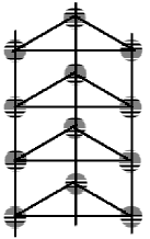
Figure 3: Three leg spin tube.

The Hamiltonian is

$$\hat{H}=J_{1}\sum^{L}_{n=1}\sum_{i=1}^{3}\hat{H}^{i,i+1}_{n,n}+J_{\perp}\sum^{L}_{n=1}\sum_{i=1}^{3}\hat{H}^{i,i}_{n,n+1}.$$ (92)

7.4 Operator for the spin tube model and the spin ladder model

Although the operators should be modified, we can apply our method to the spin ladder and spin tube. The modifications are

$$\hat{U}^{x}_{\theta}\equiv\exp{(-i\theta\hat{S}^{x}_{T})},~{}\hat{S}^{x}_{T}\equiv\sum^{L}_{n=1}\sum^{3}_{i=1}\hat{S}^{x}_{n,i}\quad\text{etc.},$$ (93)

$$\hat{U}^{\rm tw}_{\pm 2\pi}\equiv\exp{\left(\mp\frac{2\pi i}{L}\sum^{L}_{n=1}\sum^{3}_{i=1}j(\hat{S}^{z}_{n,i}-S)\right)},$$ (94)

$$\hat{P}^{\dagger}_{\rm site}\hat{S}^{x,y,z}_{n,i}\hat{P}_{\rm site}=\hat{S}^{x,y,z}_{N-n,i},$$ (95)

$$\hat{P}^{\dagger}_{\rm link}\hat{S}^{x,y,z}_{n,i}\hat{P}_{\rm link}=\hat{S}^{x,y,z}_{N-n+1,i}.$$ (96)

In the half-integer spin ladder and spin tube system, by taking the rung direction’s 3 sites as a unit-cell, we can also say that the ground states are dimer-like in the same way as the above 1D spin system. To sum up, the energy spectrum is continuous (corresponding to the Néel-like state) or gapped (corresponding to the dimer-like state) in the spin ladder and spin tube as well as the pure 1D spin system. Of course, the Néel-like state has $\hat{P}_{\rm site}=1,\hat{P}_{\rm link}=-1$ and dimer-like state has $\hat{U}^{x}_{\pi}=\hat{U}^{y}_{\pi}=\hat{U}^{z}_{\pi}=1,\hat{P}_{\rm site}=-1,\hat{P}_{\rm link}=1$ where $\hat{U}^{x}_{\pi},\hat{P}_{\rm site},\hat{P}_{\rm link}$ are defined by Eqs. (93),(95), and (96).

We point out four suitable dimer-like states in Figs. 4 and 5, and categorize with these space inversion symmetry for rung direction.

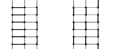
Figure 4: Spin ladder dimer-like state. Space inversion is odd, where space inversion is on the second site of the rung direction.

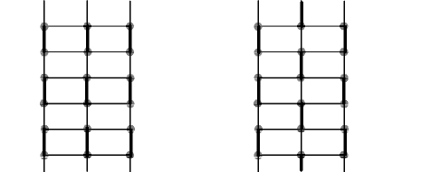
Figure 5: Space inversion is even.

And its corresponding wave functions can be written; e.g., the left one of Fig. 4 is expressed by

$$|\Psi_{dimer,l1,r1}\rangle+|\Psi_{dimer,l2,r1}\rangle+|\Psi_{dimer,l1,r2}\rangle+|\Psi_{dimer,l2,r2}\rangle:q=0$$ (97)

$$~{}|\Psi_{dimer,l1,r1}\rangle-|\Psi_{dimer,l2,r1}\rangle+|\Psi_{dimer,l1,r2}\rangle-|\Psi_{dimer,l2,r2}\rangle:q=\pi$$ (98)

where

$$|\Psi_{dimer,l1,r1}\rangle \equiv[1,1,2][1,3,4]\dots[1,L-1,L]$$

$$\times\{2,3,1\}\{2,3,2\}\dots\{2,3,L\}$$ (99)

$$|\Psi_{dimer,l2,r1}\rangle \equiv[1,2,3][1,4,5]\dots[1,L,1]$$

$$\times\{2,3,1\}\{2,3,2\}\dots\{2,3,L\}$$ (100)

$$|\Psi_{dimer,l1,r2}\rangle \equiv[1,1,2][1,3,4]\dots[1,L-1,L]$$

$$\times\{2,1,1\}\{2,1,2\}\dots\{2,1,L\}$$ (101)

$$|\Psi_{dimer,l2,r2}\rangle \equiv[1,2,3][1,4,5]\dots[1,L,1]$$

$$\times\{2,1,1\}\{2,1,2\}\dots\{2,1,L\}$$ (102)

$$[i,j,k] =\frac{1}{\sqrt{2}}(\uparrow_{j,i}\downarrow_{k,i}-\downarrow_{j,i}\uparrow_{k,i})$$

$$\{i,j,k\} =\frac{1}{\sqrt{2}}(\uparrow_{k,i}\downarrow_{k,j}-\downarrow_{k,i}\uparrow_{k,j})$$

Note $\prod_{k}\{i,j,k\}$ always has $\hat{U}^{y}_{\pi}=1,\hat{P}_{\rm site}=1,\hat{P}_{\rm link}=1$ as eigenvalues (this space inversion is the leg direction’s one), so we can easily understand that Eq. (98) has $\hat{U}^{y}_{\pi}=1,\hat{P}_{\rm site}=-1,\hat{P}_{\rm link}=1$ with the possibility of an energy gap.

7.5 Distorted diamond chain model

Our discussion can be also valid in a distorted diamond chain [20]. The Hamiltonian is

$$\hat{H}=J_{1}\sum^{N/3}_{j=1}(\hat{S}_{3j-1}\hat{S}_{3j}+\hat{S}_{3j}\hat{S}_{3j+1})+J_{2}\sum^{N/3}_{j=1}\hat{S}_{3j+1}\hat{S}_{3j+2}+J_{3}\sum^{N/3}_{j=1}(\hat{S}_{3j-2}\hat{S}_{3j}+\hat{S}_{3j}\hat{S}_{3j+2}).$$ (103)

The diamond chain has 3 sites in unit-cell like the spin ladder and spin tube. In addition, this model has space inversion symmetry. (K. Okamoto, Shibaura Institute of Technology, private communicationy) Therefore, by the same argument, the energy spectrum is gapless or gapped with dimer-like state.

7.5.1 Magnetic plateaux

In a nonzero magnetic field, the symmetry of Eq. (103) becomes from SU(2) to U(1). In the rational magnetization $M=M_{s}/3,2M_{s}/3$ ($M_{s}$ is the saturation magnetization), it is reported that magnetization plateaux appear [20], by using the level spectroscpoy and other methods. The BKT phase transition at $2M_{s}/3$ is a similar type as the S=1/2 NNN XXZ model, since the discussion of Sect. 6.2 applies for the $2M_{s}/3$ phase diagram.

8 Ground state symmetries and system size

8.1 System size $L=2n+1$

In the case of $SL$ half-integer (i.e., $S$ half-integer and $L$ odd), the relation of spin reversal operators becomes $(\hat{U}_{\pi}^{x})^{2}=(\hat{U}_{\pi}^{y})^{2}=(\hat{U}_{\pi}^{z})^{2}=-1$, and $\hat{U}_{\pi}^{x}\hat{U}_{\pi}^{y}\hat{U}_{\pi}^{z}=-1$. Therefore the sets $\{\pm\hat{1},\pm\hat{U}_{\pi}^{x},\pm\hat{U}_{\pi}^{y},\pm\hat{U}_{\pi}^{z}\}$ form the quaternion group (see Appendix A). The time reversal operator has a similar relation $\hat{K}^{2}=-1$. Thus, the algebraic structure of the $SL$ half-integer case is quite different from the $SL$ integer case.

Since we did not use the periodic boundary condition in the process of the derivation in Appendix A, we can apply $\hat{U}_{\pi}^{x}\hat{U}_{\pi}^{y}\hat{U}_{\pi}^{z}=-1$ for the $SL$ half-integer case, or $\hat{U}_{\pi}^{x}\hat{U}_{\pi}^{y}\hat{U}_{\pi}^{z}=1$ for the $SL$ integer case, also in the open boundary condition.

In the periodic boundary condition, we cannot distinguish the two types of space inversion (site inversion and link inversion) in the odd sites system. On the other hand, in the open boundary condition, only the site inversion can be defined.

8.2 System size $L=4n,4n+2$

For the nonfrustrating case, by using an MLM-type discussion [21] [22], one can prove that the ground state has $q=0,\hat{U}^{y}_{\pi}=1,\hat{P}_{\rm link}=\hat{P}_{\rm site}=1$ in $L=4n$, and $q=\pi,\hat{U}^{y}_{\pi}=1,\hat{P}_{\rm link}=-1,\hat{P}_{\rm site}=1$ in $L=4n+2$[23]. Therefore, for $L=4n+2$, we should choose $|\Psi_{g}\rangle$ as $\hat{U}_{\rm trl}|\Psi_{g}\rangle=-|\Psi_{g}\rangle,\hat{U}^{y}_{\pi}|\Psi_{g}\rangle=\hat{U}^{z}_{\pi}|\Psi_{g}\rangle=|\Psi_{g}\rangle,\hat{P}_{\rm site}|\Psi_{g}\rangle=|\Psi_{g}\rangle,\hat{P}_{\rm link}|\Psi_{g}\rangle=-|\Psi_{g}\rangle$ instead of Eq. (12), but basically our discussions for $L=4n$ are valid also in $L=4n+2$.

9 Summary and discussions

In this paper we have investigated the system with discrete symmetries: spin reversal, space inversion (link or site inversion), and time reversal symmetries. And when the system has U(1) or SU(2) continuous symmetry, we can discuss the low-lying states using the LSM theorem. In Sect. 4 we constructed four states with the twisting operators, then confirmed the discrete symmetries of them. Using the discrete symmetries, we classify the $q=\pi$ states into the dimer-like, the Néel-like, or other states. Although superficially the LSM theorem suggests both the dimer-like and the Néel-like states ($q=\pi$) are degenerate with the $q=0$ state, we have solved this dilemma by considering the normalization of the dimer-like and Néel-like states in Sect. 5, where the relation of the normalization and the gap is summarized in Table 1. In Sect. 6, we have shown that a part of the discrete symmetries, i.e., either space inversion or spin reversal or time reversal, is enough for the above arguments. Note that since the spin reversal or time reversal symmetry means zero magnetization, then the space inversion symmetry is needed to explain the magnetic plateau (see also the example in Sect. 7.5.1).

We mention the relation between the BKT type transition and the present work. As we discussed in Sect. 7.1, the classification of Table 1 is closely related with the BKT type transition. However, when the number of the degenerate ground states is more than the minimum degeneracy expected from the LSM theorem, such as the (2,2) antiphase state in Sect. 7.1, it is not necessarily related with the BKT type transition. Moreover one should classify whether the doublet state is gapped or gapless, plus the classification in Table 1.

There is caution on the statement that at least one of the ground states satisfies Eq. (12) in Sect. 2.6. This statement may remain valid in the frustrating regions with zero magnetization, including the Majumdar-Gosh model. Generally, in the rational magnetization with space inversion symmetry, a similar statement, at least one of the ground states satisfies $\hat{P}|\Psi_{g}\rangle=|\Psi_{g}\rangle$ and $q=0$, may be valid. However the above statement is violated for the irrational magnetization with frustration when the incommensurability occurs. For example, in the NNN XXZ model (90), the energy dispersion of the one spin flip from the fully aligned state ($S^{z}_{T}=SL-1$) is the double well form when $J_{1}>0,\>J_{2}/J_{1}>1/4$.

Finally, we comment on the symmetry protected topological phases (SPTP) [24][25]. Between our work and SPTP, there is a similar point of view (distinguishing the states by space inversion, spin reversal, and time reversal symmetry), however, some conditions are different (SPTP: integer spin, our work: half-integer spin). Other differences are that SPTP theory treats only the link inversion as the space inversion, whereas in our theory both the site inversion and the link inversion are considered; in our theory the magnetic plateaux in the rational magnetization have been treated.

Appendix A $Z_{2}\times Z_{2}$ spin reversal symmetry

[Lemma 1 ]. For the $SL$ integer case,

$$\hat{U}^{x}_{\pi}\hat{U}^{y}_{\pi}\hat{U}^{z}_{\pi}=\hat{U}^{x}_{2\pi}=\exp{(-2\pi i\hat{S}^{x}_{T})}=1.$$ (104)

[Proof] According to Eq. (5),

$$(\hat{U}^{x}_{\pi/2})^{\dagger}\hat{S}^{y}_{k}\hat{U}^{x}_{\pi/2}=-\hat{S}^{z}_{k}.$$ (105)

Therefore, we obtain

$$(\hat{U}^{x}_{\pi/2})^{\dagger}\hat{U}^{y}_{\pi/2}\hat{U}^{x}_{\pi/2}=(\hat{U}^{x}_{\pi/2})^{\dagger}\left[\sum_{n=0}^{\infty}\frac{(-i\pi/2)^{n}}{n!}(S^{y}_{T})^{n}\right]\hat{U}^{x}_{\pi/2}=(\hat{U}^{z}_{\pi/2})^{\dagger},$$ (106)

or

$$\hat{U}^{y}_{\pi/2}\hat{U}^{x}_{\pi/2}=\hat{U}^{x}_{\pi/2}(\hat{U}^{z}_{\pi/2})^{\dagger}.$$ (107)

Similarly we get

$$\hat{U}^{y}_{\pi/2}\hat{U}^{z}_{\pi/2}=\hat{U}^{x}_{\pi/2}\hat{U}^{y}_{\pi/2}$$ (108)

and

$$(\hat{U}^{z}_{\pi/2})^{\dagger}\hat{U}^{y}_{\pi/2}\hat{U}^{z}_{\pi/2}=\hat{U}^{x}_{\pi/2}.$$ (109)

By using Eqs. (108),(107), and (109) one after another, we obtain the product relation of spin reversal operators as

$$\hat{U}^{x}_{\pi}\hat{U}^{y}_{\pi}\hat{U}^{z}_{\pi} =\hat{U}^{x}_{\pi/2}\hat{U}^{x}_{\pi/2}\hat{U}^{y}_{\pi/2}(\hat{U}^{y}_{\pi/2}\hat{U}^{z}_{\pi/2})\hat{U}^{z}_{\pi/2}$$

$$=\hat{U}^{x}_{\pi/2}\hat{U}^{x}_{\pi/2}(\hat{U}^{y}_{\pi/2}\hat{U}^{x}_{\pi/2})\hat{U}^{y}_{\pi/2}\hat{U}^{z}_{\pi/2}$$

$$=\hat{U}^{x}_{\pi/2}\hat{U}^{x}_{\pi/2}\hat{U}^{x}_{\pi/2}[(\hat{U}^{z}_{\pi/2})^{\dagger}\hat{U}^{y}_{\pi/2}\hat{U}^{z}_{\pi/2}]$$

$$=\hat{U}^{x}_{\pi/2}\hat{U}^{x}_{\pi/2}\hat{U}^{x}_{\pi/2}\hat{U}^{x}_{\pi/2}$$

$$=\hat{U}^{x}_{2\pi}.$$ (110)

Finally, since the eigenvalue of $\hat{S}^{x}_{T}$ is integer for $SL$:integer, we can prove

$$\hat{U}^{x}_{\pi}\hat{U}^{y}_{\pi}\hat{U}^{z}_{\pi}=\hat{U}^{x}_{2\pi}=\exp{(-2\pi i\hat{S}^{x}_{T})}=1.$$ (111)

[Remarks]

(I) These spin reversal operators $\hat{U}^{x}_{\pi},\hat{U}^{y}_{\pi},\hat{U}^{z}_{\pi}$ satisfy ($\hat{U}^{x}_{\pi})^{2}=(\hat{U}^{y}_{\pi})^{2}=(\hat{U}^{z}_{\pi})^{2}=\hat{1}$ and $\hat{U}^{x}_{\pi}\hat{U}^{y}_{\pi}=\hat{U}^{z}_{\pi}$. Therefore {$\hat{1},\hat{U}^{x}_{\pi},\hat{U}^{y}_{\pi},\hat{U}^{z}_{\pi}$} form the Klein four-group, which is isomorphic to the $Z_{2}\times Z_{2}$ group.

(II) This proof does not need the translational, space inversion, and time reversal symmetries.

[Corollary 1] For the $SL$ half-integer case,

$$\hat{U}^{x}_{\pi}\hat{U}^{y}_{\pi}\hat{U}^{z}_{\pi}=-1.$$ (112)

and $(\hat{U}_{\pi}^{x})^{2}=(\hat{U}_{\pi}^{y})^{2}=(\hat{U}_{\pi}^{z})^{2}=-1$, since each of the eigenvalues $\hat{S}^{x}_{T},\hat{S}^{y}_{T},\hat{S}^{z}_{T}$ is half-integer.

Therefore $\{\pm\hat{1},\pm\hat{U}_{\pi}^{x},\pm\hat{U}_{\pi}^{y},\pm\hat{U}_{\pi}^{z}\}$ form the quaternion group.

Appendix B Translation and twisting operator

[Lemma 2 ]

$$\hat{U}^{\rm tw}_{2\pi l}\hat{U}_{\rm trl} =\hat{U}_{\rm trl}\hat{U}^{\rm tw}_{2\pi l}\exp\left(\frac{2\pi il}{L}(\hat{S}^{z}_{T}-SL)\right),$$ (113)

$$\hat{U}^{\rm twl}_{2\pi l}\hat{U}_{\rm trl} =\hat{U}_{\rm trl}\hat{U}^{\rm twl}_{2\pi l}\exp\left(\frac{2\pi il}{L}(\hat{S}^{z}_{T}-SL)\right)\quad(l:\text{integer}).$$ (114)

[Proof]

$$\hat{U}_{\rm trl}^{\dagger}\hat{U}^{\rm tw}_{2\pi l}\hat{U}_{\rm trl} =\exp\left(-\frac{2\pi il}{L}\sum_{j=1}^{L}j(\hat{S}^{z}_{j+1}-S)\right)$$

$$=\exp\left(-\frac{2\pi il}{L}\left(\sum_{j=2}^{L}(j-1)(\hat{S}^{z}_{j}-S)+L(\hat{S}^{z}_{L+1}-S)\right)\right)$$

$$=\hat{U}^{\rm tw}_{2\pi l}\exp\left(\frac{2\pi il}{L}(\hat{S}^{z}_{T}-SL)\right)\exp(-2\pi il(\hat{S}^{z}_{1}-S)),$$ (115)

where we have used $\hat{S}^{z}_{L+1}=\hat{S}^{z}_{1}$. Since the eigenvalue of $\hat{S}^{z}_{1}-S$ is an integer, we obtain Eq. (113). Similarly, we obtain Eq. (114).

Appendix C Time reversal operator

[Lemma 3 ]

$$\hat{U}^{x,y,z}_{\pi}\hat{K} =\hat{K}\hat{U}^{x,y,z}_{\pi}.$$ (116)

[Proof]

$$\hat{K}^{\dagger}\hat{U}^{x,y,z}_{\pi}\hat{K} =\hat{K}^{\dagger}\left(\sum_{n=0}^{\infty}[\{\pi i\sum^{L}_{j=1}(\hat{S}^{x,y,z}_{j})\}^{n}/n!]\right)\hat{K}$$

$$=\sum_{n=0}^{\infty}[\{-\pi i\sum^{L}_{j=1}(-\hat{S}^{x,y,z}_{j})\}^{n}/n!]=\hat{U}^{x,y,z}_{\pi}.$$ (117)

[Lemma 4 ] For the $SL$ integer case,

$$\hat{U}^{\rm tw}_{2\pi l}\hat{K} =(-1)^{2Sl}\hat{K}\hat{U}^{\rm tw}_{2\pi l},$$ (118)

$$\hat{U}^{\rm twl}_{2\pi l}\hat{K} =\hat{K}\hat{U}^{\rm twl}_{2\pi l}\qquad(l:\text{integer}).$$ (119)

[Proof]

$$\hat{K}^{\dagger}\hat{U}^{\rm tw}_{2\pi l}\hat{K} =\hat{K}^{\dagger}\left(\sum_{n=0}^{\infty}[\{-\frac{2\pi il}{L}\sum^{L}_{j=1}j(\hat{S}^{z}_{j}-S)\}^{n}/n!]\right)\hat{K}$$

$$=\sum_{n=0}^{\infty}[\{\frac{2\pi il}{L}\sum^{L}_{j=1}j(-\hat{S}^{z}_{j}-S)\}^{n}/n!]$$

$$=\exp\left(-\frac{2\pi il}{L}\sum^{L}_{j=1}j(\hat{S}^{z}_{j}-S)\right)\exp\left(-\frac{2\pi il}{L}2S\sum^{L}_{j=1}j\right)$$

$$=\exp(-2\pi ilS(L+1))\hat{U}^{\rm tw}_{2\pi l}=(-1)^{2Sl}\hat{U}^{\rm tw}_{2\pi l},$$ (120)

where we have used the condition $SL$: integer. Similarly, we calculate

$$\hat{K}^{\dagger}\hat{U}^{\rm twl}_{2\pi l}\hat{K}=\exp(-2\pi ilSL)\hat{U}^{\rm twl}_{2\pi l}=\hat{U}^{\rm twl}_{2\pi l}.$$ (121)

References

• [1] E.Lieb,T.Schultz, and D.Mattis, Ann. Phys. 16, 407, (1961)
• [2] K.Nomura,J.Morishige, and T.Isoyama, J. Phys. A 48, 375001 (2015).
• [3] I. Affleck and E.H.Lieb, Lett. in Math. Phys. 12, 57 (1986).
• [4] M.Kolb, Phys.Rev.B 31, 7494 (1985).
• [5] M. Oshikawa, M. Yamanaka, and I. Affleck, Phys. Rev. Lett. 78, 1984 (1997).
• [6] C. K. Majumdar and D. K. Ghosh, J. Math. Phys. 10, 1388 (1969).
• [7] C. K. Majumdar: J. Phys. C 3, 911 (1970).
• [8] B. S. Shastry and B. Sutherland, Phys. Rev. Lett. 47, 964 (1981).
• [9] K. Nomura and K. Okamoto, J. Phys. Soc. Jpn. 62, 1123 (1993).
• [10] K. Nomura and K. Okamoto, J. Phys. A 27, 5773 (1994).
• [11] K. Nomura and A. Kitazawa, J. Phys. A 31, 7341 (1998).
• [12] K. Okamoto and K. Nomura, Phys. Lett. A 169, 433 (1992).
• [13] J. Igarashi and T. Tonegawa, Phys. Rev. B 40, 756 (1989).
• [14] C. Itoi and S. Qin, Phys. Rev. B 63, 224423, (2001).
• [15] S. Furukawa, M. Sato, S. Onoda, and A. Furusaki, Phys. Rev. B, 86, 094417 (2012).
• [16] H. Suzuki, and K. Takano, J. Phys. Soc. Jpn. 77, 113701 (2008).
• [17] T. Hamada, J. Kane, S. Nakagawa, and Y. Natsume, J. Phys. Soc. Jpn. 57, 1891 (1988).
• [18] K.Kawano,M.Takahashi, J. Phys. Soc. Jpn. 66, 4001 (1997).
• [19] Y.Fuji,S.Nishimoto,H.Nakada,M.Oshikawa, Phys.Rev.B 89, 054425 (2014).
• [20] K. Okamoto, T. Tonegawa, M. Kaburagi, J. Phys. Condens. 15, 5979 (2003).
• [21] W. Marshall, Proc. Roy. Soc. A232, 48 (1955).
• [22] E. H. Lieb and D. Mattis, J. Math. Phys. 3, 749 (1962).
• [23] K BΓ€rwinkel,H.-J Schmidt, and J Schnack, J. Magn. Mater. 220, 227 (2000).
• [24] F. Pollmann, A. M. Turner, E. Berg, M. Oshikawa, Phys. Rev. B 81, 064439 (2010).
• [25] F. Pollmann, E. Berg, A. M. Turner, M. Oshikawa, Phys. Rev. B 85, 075125 (2012).