Adaptive cyclically dominating game on co-evolving networks: Numerical and analytic results

Abstract

A co-evolving and adaptive Rock (R)-Paper (P)-Scissors (S) game (ARPS) in which an agent uses one of three cyclically dominating strategies is proposed and studied numerically and analytically. An agent takes adaptive actions to achieve a neighborhood to his advantage by rewiring a dissatisfying link with a probability $\displaystyle p$ or switching strategy with a probability $\displaystyle 1-p$. Numerical results revealed two phases in the steady state. An active phase for $\displaystyle p<p_{\text{cri}}$ has one connected network of agents using different strategies who are continually interacting and taking adaptive actions. A frozen phase for $\displaystyle p>p_{\text{cri}}$ has three separate clusters of agents using only R, P, and S, respectively with terminated adaptive actions. A mean-field theory of link densities in co-evolving network is formulated in a general way that can be readily modified to other co-evolving network problems of multiple strategies. The analytic results agree with simulation results on ARPS well. We point out the different probabilities of winning, losing, and drawing a game among the agents as the origin of the small discrepancy between analytic and simulation results. As a result of the adaptive actions, agents of higher degrees are often those being taken advantage of. Agents with a smaller (larger) degree than the mean degree have a higher (smaller) probability of winning than losing. The results are useful in future attempts on formulating more accurate theories.

I Introduction

Agent-based modelling is an important tool for studying the autonomous actions of individual entities and their interactions review_szabo ; review_statphy in complex systems. The interactions often reflect how agents compete, especially in the context of competing games. Examples of some extensively studied games are the prisoner’s dilemma (PD), snowdrift game (SG), and stag hunt game (SH) review_szabo ; book_evolutionary ; book_sh ; book_axelrod . These are two-strategy games with agents having a choice of two possible options. In the present work, we focus on the Rock-Paper-Scissors (RPS) game review_szabo ; book_evolutionary ; review_rps , characterized by three strategies that dominate each other cyclically. Depending on the context, the strategy of an agent can be regarded as his state, character, opinion or species. The strategies are related cyclically through: Rock (R) crushes Scissors (S), Scissors (S) cuts Paper (P), and Paper (P) covers Rock (R) review_szabo ; review_rps ; review_zhou . Despite its simplicity, many phenomena in nature can be described within the framework of RPS game. A well-known example is related to the mating strategy of the common side-blotched lizards (Uta stansburiana), a species of lizards found in the western coast of North America rps_lizard . Other examples include phenomena in marine ecological communities rps_marine , coexistence of different kinds of microbes rps_bacteria ; rps_bacteria2 ; rps_bacteria3 , and in chemical and biological systems review_szabo ; review_rps ; review_zhou ; rps_grass . There are phenomena in economic and social systems, e.g., human decision-making processes and epidemic diseases, that also involve cyclical dominance and they can be studied within the RPS framework review_szabo ; review_zhou ; rps_exp .

An interesting question is how network structures review_szabo ; review_rps affect the RPS game. The focus so far has been on static networks, i.e., the links connecting two competing agents are fixed. For RPS agents interact in a square lattice tainaka94 with the loser updating the strategy to be that of the winner, spatial self-organized patterns emerged. Szabó et al. studied the small-world effect on RPS game by replacing a fraction $\displaystyle r$ of the links in a square lattice by links that connect two randomly selected agents rps_szabo1 . It was found that two qualitatively different phases result, depending on the value of $\displaystyle r$. Szolnoki and Szabó studied the RPS game in Kagome, honeycomb, triangular, cubic, and ladder-shape lattices rps_szabo2 . They found that while the spatial dimension of the lattices affects the transitions between different phases strongly, the clustering coefficient does not.

Going beyond static networks, co-evolving networks have attracted much attention in recent years review_szabo ; review_statphy ; review_rps ; review_tgross ; review_mini . In co-evolving networks, an agent may switch his strategy or alter his competing neighbors so as to attain an environment that is to his advantage. Such adaptive actions couple the dynamics of strategy selections and network evolution. Co-evolving networks invoking PD, SG, SH games have been studied review_szabo ; review_statphy ; review_tgross ; review_mini ; dasg1 ; Xu1 . In particular, the present work is motivated by the two-option adaptive co-evolving voter model vm and the dissatisfied adaptive snowdrift game dasg1 ; dasg2 . In the co-evolving voter model vm , there are two opposite opinions competing for dominance in an initially random regular network and agents prefer to be surrounded by like-opinion neighbors. When an agent interacts with a randomly chosen neighbor of the opposite opinion, he has a probability $\displaystyle p$ to cut the link to the neighbor and rewire it to a randomly chosen agent of the same opinion. With a probability $\displaystyle 1-p$, the agent is convinced by the neighbor and switches to the opposite opinion. Both actions are rational in that the agents tend to pursue local consensus. Despite its simplicity, the phenomena are rich. For values of $\displaystyle p$ below (above) a critical value, the system evolves into an active (a frozen) phase in which the network evolution and strategy selection continue (cease). Similar adaptive actions (i.e. switching strategies and rewiring the links to dissatisfying neighbors) were included in the model of dissatisfied adaptive snowdrift game (DASG) dasg1 ; dasg2 . In DASG, adaptive actions are taken when agents become dissatisfied with non-cooperative neighbors. The resulting network is either in a disconnected, dynamically frozen, and character-segregated phase or a connected, dynamical, and character-mixed phase, depending on a payoff parameter. Analytic approaches to co-evolving networks require careful treatment of spatial correlations ji . Other examples in which similar adaptive actions are invoked include a reversed opinion-formation model reverse and an inverse voter model inverse ; CWChoi . Networking effects, including co-evolving networks, also pose challenging questions to analytic approaches. Typically approaches such as mean field approximation and pair approximation review_szabo ; review_rps often only give results in qualitative agreement with simulations review_szabo ; vm ; dasg1 ; dasg2 ; inverse ; ji ; CWChoi . The reason is that the adaptive actions are sensitive to the local competing environment and thus spatial correlations are important. We have made various attempts in understanding the key factors in formulating theories that better capture spatial correlations dasg2 ; ji ; CWChoi ; WZhang1 ; WZhang2 ; Elvis . An improved mean field theory was shown to give good results for DASG ji and the inverse voter model CWChoi .

Here, we generalize the study of adaptive co-evolving models to cyclic multiple-strategy case. In particular, an adaptive and co-evolving RPS model, abbreviated as APRS, is proposed and studied in detail. Our model is different from the adaptive RPS model studied by Demirel et al. arps . The agents in adaptive RPS model prefers to have neighbors of the same option by an adaptive mechanism in which an agent who lost a RPS game adopts the strategy of the winner or to seek a new neighbor of the same opinion. The authors focused on the time evolution of the fractions of agents using the different strategies. In our model, the agents take adaptive actions to enhance their chance of winning. We focus on the different phases exhibited in the steady state and the formulation of analytic approaches. In Sec. 2, we define our model and identify the key features as revealed by simulations. The model is parameterized by a probability $\displaystyle p$ of rewiring an unfavorable link. The system evolves to two different phases for different ranges of $\displaystyle p$. In Sec. 3, a theory based on the densities of different kinds of links connecting agents of different strategies is constructed. Results are found to be in good agreement with simulations, with small yet noticeable discrepancies. In Sec. 4, we point out that the small discrepancies are important hints for studying the validity of the assumptions in a theory. We analyze the dependence of the probabilities of winning and losing of different types of agents. These probabilities are found to depend on the role of an agent in an adaptive process and his degree. These features are usually not included in analytic approaches. Although the context of ARPS is studied, the discussions on the formalism of mean field theory and its validity are intentionally carried out in a general form. As such, the analysis here can be readily applied to other co-evolving network models with two or more options or strategies. Results are summarized in Sec. 5.

II Adaptive Rock-Paper-Scissors model and Key Features

Consider a system of $\displaystyle N$ agents. For concreteness, the agents are initially connected via a random regular graph of uniform degree $\displaystyle\mu$ and each of them is assigned one of the three strategies (R, P, or S) with equal probabilities. In a time step, an agent, referred to as the active agent, is selected randomly. If there is no connected neighbor, i.e. of degree zero, there will be no action and the time step ends. Otherwise, the active agent selects a connected neighbor, referred to as the passive agent, at random. They interact via a RPS game. If the active agent wins or there is a draw, he is satisfied and no adaptive actions take place. If the active agent loses, he is dissatisfied and he will take one of the following adaptive actions: (i) with a probability $\displaystyle p$ to cut the link to the passive agent and rewire it to another agent (called the rewiring target) randomly chosen from all the agents in the system who are not a neighbor, or (ii) with a probability $\displaystyle(1-p)$ to switch his strategy to the one that can defeat the passive agent. Figure 1 illustrates the possible events and adaptive actions in a time step with examples. As one active agent is picked at a time step, the interactions are asynchronous. The probability $\displaystyle p$ is the only parameter in APRS. The adaptive actions are rational in that an agent always aims to prevent losing to the same opponent by altering the local competing environment. They drive the strategies employed by the agents and the network connections to co-evolve. The process continues until the network achieves a macroscopically steady state.

The long-time behavior of the system can be characterized by a few macroscopic quantities. They include the fractions $\displaystyle f_{R}$, $\displaystyle f_{P}$, and $\displaystyle f_{S}$ of agents using the strategies-R, P, and S, respectively, the fractions of undirected inert links $\displaystyle l_{RR}$, $\displaystyle l_{PP}$ and $\displaystyle l_{SS}$ connecting agents using the same strategy that would lead to a draw, and the fractions of undirected active links $\displaystyle l_{RP}$, $\displaystyle l_{PS}$ and $\displaystyle l_{SR}$ connecting agents using different strategies that would lead to a win-lose situation. It should be pointed out that ARPS can be implemented with different initial strategy assignments and initial network connections. Here, we take advantage of the simplicity provided by random initial strategy assignments and the symmetry among the three strategies so that we could focus on the discussion of the $\displaystyle p$-dependence of two link densities, one for inert and the other for active links.

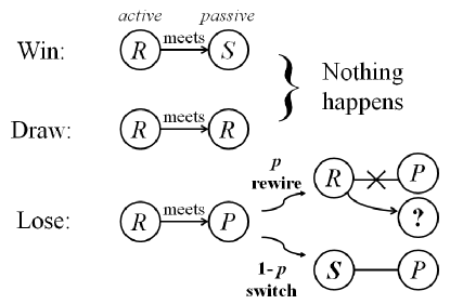
Figure 1: Schematic illustrations of the adaptive actions of an active agent.

Detailed numerical simulations were carried out for ARPS. Here we focus on an initial network of uniform degree $\displaystyle\mu=2$ and $\displaystyle N=10,000$ agents. The results illustrated that $\displaystyle f_{R}=f_{P}=f_{S}=1/3$, $\displaystyle l_{RR}=l_{PP}=l_{SS}$ and $\displaystyle l_{RP}=l_{PS}=l_{SR}$. These are expected as no strategy plays a special role in RPS and the adaptive actions in ARPS. The random initial conditions make sure that all strategies are evenly present. This allows us to focus the discussion on how $\displaystyle l_{RR}(p)$ and $\displaystyle l_{RP}(p)$ behave at long time. Fig. 2 shows the simulation results (symbols). Fig. 2(a) confirms $\displaystyle f_{R}=f_{P}=f_{S}=1/3$ for all values of $\displaystyle p$, as expected from symmetry consideration. Fig. 2(b) shows the behavior of $\displaystyle l_{RR}(p)$ (squares) and $\displaystyle l_{RP}(p)$ (circles). These quantities reveal the two different phases classified by $\displaystyle p$. For $\displaystyle 0<p<p_{\text{cri}}$, $\displaystyle l_{RR}$ increases monotonically with $\displaystyle p$ and approaches $\displaystyle l_{RR}=1/3$ at $\displaystyle p=p_{\text{cri}}$ continuously while $\displaystyle l_{RP}$ drops monotonically with $\displaystyle p$ and vanishes continuously at $\displaystyle p=p_{\text{cri}}$. In the range $\displaystyle p_{\text{cri}}<p<1$, $\displaystyle l_{RR}=1/3$ and $\displaystyle l_{RP}=0$. We found that $\displaystyle p_{\text{cri}}\approx 0.78$ for $\displaystyle\mu=2$. We also studied initial networks of different values of $\displaystyle\mu$. The results show the same qualitative behavior, but $\displaystyle p_{\text{cri}}$ increases with $\displaystyle\mu$. For example, $\displaystyle p_{\text{cri}}\approx 0.89$ for $\displaystyle\mu=4$. Here, we focus on analyzing the results for $\displaystyle\mu=2$.

Figure 2: Simulation (symbols) of (a) $\displaystyle f_{R}$ and (b) $\displaystyle l_{RR}$ and $\displaystyle l_{RP}$ in the steady state as a function of the rewiring probability $\displaystyle p$. The data are obtained by averaging results over 300 independent runs. The system has $\displaystyle N=10000$ agents and a mean degree $\displaystyle\mu=2$. The two phases are indicated in (b). Results of mean field theory as given by Eqs.(10) and (11) are included (lines) for comparison.

For $\displaystyle p<p_{\text{cri}}$, the system has active links and it is in the active phase. These active links promote agents’ interactions and adaptive actions. This is a dynamic phase as strategy switching and network rewiring persist. For $\displaystyle p>p_{\text{cri}}$, the system has only inert links and it is in an inactive and frozen phase. There is no more adaptive action. The two phases also differ drastically in network structure. In the active phase, the system has a main cluster consisting of agents using the three strategies with both active and inert links. In the frozen phase, the system breaks into three segregated pure-strategy clusters of equal size, with each cluster having agents using only R, P, or S. Another noticeable feature is the discontinuous jump from $\displaystyle l_{RP}=2/9$ at $\displaystyle p=0$ to a larger value when $\displaystyle p$ becomes finite. There is a similar discontinuous jump from $\displaystyle l_{RR}=1/9$ at $\displaystyle p=0$ to a smaller value. These discontinuities will be discussed in Sec. 4.

III Mean-field approach

Inspired by previous analytic approaches vm ; dasg1 ; dasg2 ; inverse ; ji ; CWChoi for co-evolving agent-based models, we formulate a theory by tracing the expected changes in the macroscopic quantities in a time step. In principle, the system has many macroscopic variables. At the single-agent level, we have the fractions $\displaystyle f_{R}$, $\displaystyle f_{P}$, and $\displaystyle f_{S}$. At the two-agent or link level, there are the link densities $\displaystyle l_{RR}$, $\displaystyle l_{PP}$, $\displaystyle l_{SS}$, $\displaystyle l_{RP}$, $\displaystyle l_{PS}$ and $\displaystyle l_{SR}$. As discussed, symmetry implies $\displaystyle{l_{RR}}={l_{PP}}={l_{SS}}$ and $\displaystyle{l_{RP}}={l_{PS}}={l_{SR}}$. Therefore, we could take $\displaystyle l_{RR}$ and $\displaystyle l_{RP}$ as variables. Together with $\displaystyle{f_{R}}={f_{P}}={f_{S}}=1/3$, the two variables obey $\displaystyle l_{RR}+l_{RP}=1/3$. This sum rule is also demonstrated by the simulation results in Fig. 2(b). As a result, a single variable suffices for a theory up to the level of links. We choose $\displaystyle l_{RP}$ as the variable, although other choices can also be made.

We formulate a theory in a way that can be readily generalized to other co-evolving network problems. To proceed, we aim at writing down an equation for the change $\displaystyle\Delta l_{RP}$ in $\displaystyle l_{RP}$ in a time step. Based on the adaptive actions, $\displaystyle\Delta l_{RP}$ is determined by: (i) the strategy of the active agent, (ii) his local configuration including the degree $\displaystyle\kappa$ and the numbers of neighbors using the different strategies, (iii) the probability of losing the RPS game, (iv) the adaptive action taken after losing, (v) the change in the number of links $\displaystyle\Delta L_{RP}$ connecting an agent using strategy-R and an agent using strategy-P (called RP-links) due to the adaptive action. Table 1 gives the possible values of $\displaystyle\Delta L_{RP}$ due to the adaptive actions. Schematically, the expected change in the link density $\displaystyle\Delta l_{RP}$ can be expressed in terms of the probabilities of all possible local configurations, strategies and adaptive actions, and the corresponding local changes in the number of RP-links as follows:

$$\displaystyle\Delta l_{RP}=\sum\limits_{X=R,P,S}f_{X}\sum\limits_{\kappa}P_{X}(\kappa)\sum\limits_{\lambda_{XY},\lambda_{XZ}}Q_{X,\kappa}(\lambda_{XY},\lambda_{XZ})\frac{\lambda_{XY}}{\kappa}\left[\frac{p\Delta L_{RP}^{\text{rewire}}}{L_{\text{total}}}+\frac{(1-p)\Delta L_{RP}^{\text{switch}}}{L_{\text{total}}}\right].$$ (1)

Here, $\displaystyle P_{X}(\kappa)$ is the probability of an agent using strategy-X and having degree $\displaystyle\kappa$, Y (Z) is the strategy which wins over (loses to) X, $\displaystyle Q_{X,\kappa}(\lambda_{XY},\lambda_{XZ})$ is the probability of an agent using strategy-X and having degree $\displaystyle\kappa$ to have $\displaystyle\lambda_{XY}$ XY-links and $\displaystyle\lambda_{XZ}$ XZ-links, $\displaystyle\Delta L_{RP}^{\text{rewire}}$ ($\displaystyle\Delta L_{RP}^{\text{switch}}$) is the local change in RP-links due to rewiring (switching) with its possible values listed in Table 1, and $\displaystyle L_{\text{total}}=\mu N/2$ is the total number of links in the network.

Adaptive action	Change in RP-links ($\displaystyle\Delta L_{RP}$)
switch strategy from R to S	$\displaystyle-\lambda_{RP}$
switch strategy from S to P	$\displaystyle\lambda_{SR}$
switch strategy from P to R	$\displaystyle\kappa-2{\lambda_{RP}}-{\lambda_{PS}}$
agent of R cuts P then rewires to R	$\displaystyle-1$
agent of R cuts P then rewires to S	$\displaystyle-1$
agent of P cuts S then rewires to R	$\displaystyle+1$
other actions	$\displaystyle 0$

Table 1: Changes in the number of RP-links for different adaptive actions.

Eq. (1) is general but hard to solve. Formally, the quantities in the right-hand side changes with time as the adaptive actions proceed, and dynamical equations tracing their variations should also be established. Fortunately, simplifications are possible when we focus only on the long time behavior when various quantities become stable in time and close the equation by proper approximations. Eq. (1) can be written into three terms, each corresponding to the active agent using X = R, P, S, respectively, i.e.,

$$\Delta{l_{RP}}=\frac{2}{{\mu N}}\left({{f_{R}}\Delta l_{RP}^{R}+{f_{P}}\Delta l_{RP}^{P}+{f_{S}}\Delta l_{RP}^{S}}\right).\\$$ (2)

For given strategy-X and value of $\displaystyle\kappa$, there is an expected value

$$\sum\limits_{\lambda_{XY},\lambda_{XZ}}Q_{X,\kappa}(\lambda_{XY},\lambda_{XZ})(\cdots)\equiv\langle\cdots\rangle_{\lambda|X,\kappa}$$ (3)

for the agents using strategy-X and having exactly degree $\displaystyle\kappa$ to be carried out. The notation $\displaystyle\langle\cdots\rangle_{\lambda|X,\kappa}$ stresses two points: (i) the average is taken over possible $\displaystyle\lambda$’s and (ii) the result is a function of X and $\displaystyle\kappa$. Similarly, we further define an expected value over possible values of the degrees for agents using strategy-X as:

$$\sum\limits_{\kappa}{{P_{X}}(\kappa)(\cdots)}\equiv{\langle\cdots\rangle_{\kappa|X}}\;,$$ (4)

with the result depending on the strategy-X. The quantities $\displaystyle\Delta l_{RP}^{R}$, $\displaystyle\Delta l_{RP}^{P}$, and $\displaystyle\Delta l_{RP}^{S}$ in Eq. (2) can be expressed in terms of these expected values. Explicitly, they can be expressed by using Table 1 as

$$\displaystyle\Delta l_{RP}^{R} \displaystyle= \displaystyle-p\left({{f_{R}}+{f_{S}}}\right){\left\langle{\frac{{{{\left\langle{{\lambda_{RP}}}\right\rangle}_{\lambda|R,\kappa}}}}{\kappa}}\right\rangle_{\kappa|R}}-(1-p){\left\langle{\frac{{{{\left\langle{{\lambda_{RP}}^{2}}\right\rangle}_{\lambda|R,\kappa}}}}{\kappa}}\right\rangle_{\kappa|R}},$$

$$\displaystyle\Delta l_{RP}^{P} \displaystyle= \displaystyle p{f_{R}}{\left\langle{\frac{{{{\left\langle{{\lambda_{PS}}}\right\rangle}_{\lambda|P,\kappa}}}}{\kappa}}\right\rangle_{\kappa|P}}$$

$$\displaystyle+(1-p)\left(\left\langle\left\langle\lambda_{PS}\right\rangle_{\lambda|P,\kappa}\right\rangle_{\kappa|P}-2\left\langle\frac{{{{\left\langle{{\lambda_{PS}}{\lambda_{RP}}}\right\rangle}_{\lambda|P,\kappa}}}}{\kappa}\right\rangle_{\kappa|P}-\left\langle{\frac{{{{\left\langle{{\lambda_{PS}}^{2}}\right\rangle}_{\lambda|P,\kappa}}}}{\kappa}}\right\rangle_{\kappa|P}\right)\,,$$

$$\displaystyle\Delta l_{RP}^{S} \displaystyle= \displaystyle(1-p){\left\langle{\frac{{{{\left\langle{{\lambda_{SR}}^{2}}\right\rangle}_{\lambda|S,\kappa}}}}{\kappa}}\right\rangle_{\kappa|S}}\,,$$ (5)

where the terms proportional to $\displaystyle p$ are due to rewiring and those proportional to $\displaystyle(1-p)$ are due to strategy switching.

To proceed, we make approximations to the expected values so as to close the equations. Firstly, the equations can be simplified by the symmetry of the three strategies. As a result, it is sufficient to consider the expected values in regard to only one of the strategies. Without loss of generality, we retain averages over agents using strategy-R. The other expected values for strategies-P and S are given by: $\displaystyle\left\langle\left\langle\lambda_{PS}\right\rangle_{\lambda|P,\kappa}/\kappa\right\rangle_{\kappa|P}=\left\langle\left\langle\lambda_{RP}\right\rangle_{\lambda|R,\kappa}/\kappa\right\rangle_{\kappa|R}$, $\displaystyle\left\langle\left\langle\lambda_{PS}^{2}\right\rangle_{\lambda|P,\kappa}/\kappa\right\rangle_{\kappa|P}=\left\langle\left\langle\lambda_{SR}^{2}\right\rangle_{\lambda|S,\kappa}/\kappa\right\rangle_{\kappa|S}=\left\langle\left\langle\lambda_{RP}^{2}\right\rangle_{\lambda|R,\kappa}/\kappa\right\rangle_{\kappa|R}$, and $\displaystyle\left\langle\left\langle\lambda_{PS}\lambda_{RP}\right\rangle_{\lambda|P,\kappa}/\kappa\right\rangle_{\kappa|P}=\left\langle\left\langle\lambda_{RP}\lambda_{SR}\right\rangle_{\lambda|R,\kappa}/\kappa\right\rangle_{\kappa|R}$. Secondly, the expected values can be expressed in terms of the macroscopic quantities (link densities and fractions) that we want to solve. The expected values $\displaystyle{{\left\langle{{{\left\langle{{\lambda_{XY}}}\right\rangle}_{\lambda|X,\kappa}}}\right\rangle}_{\kappa|X}}$ and $\displaystyle\langle\kappa\rangle_{\kappa|X}$ are readily given by

$$\begin{array}[]{l}{{\left\langle{{{\left\langle{{\lambda_{XY}}}\right\rangle}_{\lambda|X,\kappa}}}\right\rangle}_{\kappa|X}}=\frac{\mu}{2f_{X}}\,l_{XY}\\ \langle\kappa\rangle_{\kappa|X}=\frac{\mu}{2f_{X}}\left({{l_{XY}}+{l_{XZ}}+2{l_{XX}}}\right)\,.\end{array}$$ (6)

The first equation follows from $\displaystyle l_{XY}=\frac{2}{\mu N}n_{X}\langle\lambda_{XY}\rangle_{X}$, where $\displaystyle n_{X}$ is the number of agents using strategy-X. It says that the total number of XY-links is given by the product of $\displaystyle n_{X}$ and the average number of XY-links per agent using strategy-X. The second equation relates the mean degree $\displaystyle\langle\kappa\rangle_{\kappa|X}$ among agents using strategy-X to the link densities.

For agents using strategy-R of a certain degree $\displaystyle\kappa$, the first moment $\displaystyle{\left\langle{\lambda_{RP}}\right\rangle}_{\lambda|R,\kappa}$ and the second moment $\displaystyle{\left\langle{\lambda_{RP}^{2}}\right\rangle_{\lambda|R,\kappa}}$ are related to the expected value and the variance of $\displaystyle\lambda_{RP}$ respectively, and the mixed moment $\displaystyle{\left\langle{{\lambda_{RP}}\cdot{\lambda_{SR}}}\right\rangle_{\lambda|R,\kappa}}$ is related to the covariance of $\displaystyle\lambda_{RP}$ and $\displaystyle\lambda_{SR}$ via stat1

$$\begin{array}[]{l}\left\langle{\lambda_{RP}}\right\rangle_{\lambda|R,\kappa}=\text{E}(\lambda_{RP})\\ {\left\langle{\lambda_{RP}^{2}}\right\rangle_{\lambda|R,\kappa}=\text{var}(\lambda_{RP})+\left\langle\lambda_{RP}\right\rangle_{\lambda|R,\kappa}^{2}}\\ {\left\langle{{\lambda_{RP}}\cdot{\lambda_{SR}}}\right\rangle_{\lambda|R,\kappa}=\text{cov}({\lambda_{RP}},{\lambda_{SR}})+\left\langle\lambda_{RP}\right\rangle_{\lambda|R,\kappa}\left\langle\lambda_{SR}\right\rangle_{\lambda|R,\kappa}}\;.\end{array}$$ (7)

We invoke a trinomial closure scheme to handle $\displaystyle\text{E}(\lambda_{RP})$, $\displaystyle\text{var}(\lambda_{RP})$ and $\displaystyle\text{cov}({\lambda_{RP}},{\lambda_{SR}})$ and close the equations. It is an extension of the binomial closure scheme in two-strategy models vm ; dasg2 ; ji ; inverse . The essence is to treat averages $\displaystyle\langle\cdots\rangle_{\lambda|X,\kappa}$ that involve the sums $\displaystyle\sum_{\lambda_{XY},\lambda_{XZ}}Q_{X,\kappa}(\lambda_{XY},\lambda_{XZ})(\cdots)$ approximately. Physically, $\displaystyle Q_{X,\kappa}(\lambda_{XY},\lambda_{XZ})$ is the probability of having exactly $\displaystyle\lambda_{XY}$ XY-links, $\displaystyle\lambda_{XZ}$ XZ-links and $\displaystyle(\kappa-\lambda_{XY}-\lambda_{XZ})$ XX-links, giving an agent with $\displaystyle\kappa$ neighbors using the strategy-X. This echoes the question on the distribution of three possible outcomes $\displaystyle i=1,2,3$, each occurring with the probability $\displaystyle p_{i}$, in $\displaystyle n$ independent trials. The resulting trinomial distribution gives the expected numbers $\displaystyle np_{i}$ for the three outcomes, with the variances given by $\displaystyle np_{i}(1-p_{i})$ and the covariances between different outcomes $\displaystyle i$ and $\displaystyle j$ given by $\displaystyle-np_{i}p_{j}$ stat1 ; stat2 . Here, the degree $\displaystyle\kappa$ plays the role of $\displaystyle n$. The probabilities $\displaystyle p_{1}$, $\displaystyle p_{2}$ and $\displaystyle p_{3}$ are the conditional probabilities of encountering a neighbor using strategies-R, P and S respectively, given the strategy-X of an agent of degree $\displaystyle\kappa$. Re-defining the symbols of the probabilities as $\displaystyle{\rho_{R|X,\kappa}}$, $\displaystyle{\rho_{P|X,\kappa}}$ and $\displaystyle{\rho_{S|X,\kappa}}$ respectively and invoking the trinomial closure scheme, we have

$$\begin{array}[]{l}\left\langle{\lambda_{RP}}\right\rangle_{\lambda|R,\kappa}=\kappa\cdot{\rho_{P|R,\kappa}}\\ \left\langle{\lambda_{RP}^{2}}\right\rangle_{\lambda|R,\kappa}=\kappa\cdot{\rho_{P|R,\kappa}}\left(1-{\rho_{P|R,\kappa}}\right)+\left(\kappa\cdot\rho_{P|R,\kappa}\right)^{2}\\ \left\langle{{\lambda_{RP}}\cdot{\lambda_{SR}}}\right\rangle_{\lambda|R,\kappa}=\kappa\cdot\rho_{P|R,\kappa}\cdot\rho_{S|R,\kappa}\left(-1+\kappa\right)\;.\end{array}$$ (8)

To express all quantities in terms of the link densities, we make the further approximation

$$\rho_{Y|X,\kappa}=\frac{l_{XY}}{2l_{XX}+l_{XY}+l_{XZ}}$$ (9)

that the probability $\displaystyle\rho_{Y|X,\kappa}$ is given by the fraction of out-going XY-links pointing to the neighbors using strategy-Y from all agents using strategy-X. Note that this assumption does not distinguish between different degrees $\displaystyle\kappa$ as $\displaystyle\rho_{Y|X,\kappa}$ is independent of $\displaystyle\kappa$.

Finally, using Eqs. (III), (8), and (9) allows us to express all the quantities in Eq. (2) in terms of a link density and thus close the equation. The expected value in Eq. (2) vanish at long time. Setting the resulting equation to zero gives the link density $\displaystyle l_{RP}$ as a function of the rewiring probability $\displaystyle p$. The non-trivial solution of $\displaystyle l_{RP}(p)$ is found to be

$$l_{RP}(p)=\frac{2}{9}\left(1-\frac{p}{3(\mu-1)(1-p)}\right)=\frac{2}{9p_{\text{cri}}}\frac{p_{\text{cri}}-p}{1-p}$$ (10)

for $\displaystyle p<p_{\text{cri}}$ with

$$p_{\text{cri}}=\frac{3(\mu-1)}{3\mu-2}\;,$$ (11)

and $\displaystyle l_{RP}(p)=0$ for $\displaystyle p>p_{\text{cri}}$. Results for $\displaystyle l_{RR}(p)$ follow form $\displaystyle l_{RR}(p)+l_{RP}(p)=1/3$.

The analytic results in Eqs. (10) and (11) are shown in Fig. 2(b) (lines) for comparison for the case of $\displaystyle\mu=2$. The results and the simulation results are in good agreement. The theory captures the two phases and the behavior of the phase transition. There are slight discrepancies near the phase transition. The theory predicts that $\displaystyle p_{\text{cri}}=3/4$ for $\displaystyle\mu=2$, which is slightly lower than $\displaystyle p_{\text{cri}}\approx 0.78$ obtained by numerical simulations. The theory predicts a shift in $\displaystyle p_{\text{cri}}$ to a higher value with increasing $\displaystyle\mu$, which is a feature also observed in numerical simulations.

IV Active agents win more than passive agents via co-evolving mechanism

The discrepancies between analytic and simulation results, despite small, reveals important information on the validity of the assumptions in the mean-field approach and the effects of the co-evolving mechanism, as we now show. In every turn, the active agent may win, lose, or draw. Recording the probabilities of winning, losing, and drawing of the active agents over many rounds, the averages $\displaystyle\overline{f}_{\text{win}}$, $\displaystyle\overline{f}_{\text{draw}}$ and $\displaystyle\overline{f}_{\text{lose}}$ of these probabilities for the active agents can be obtained. Due to the cyclic symmetry of the strategies, we could focus on any strategy for an active agent, say R, and express the three probabilities as follows:

$$\begin{array}[]{l}\overline{f}_{\text{win}}={\left\langle\left\langle{\frac{{{\lambda_{SR}}}}{\kappa}}\right\rangle_{\lambda|R,\kappa}\right\rangle_{\kappa|R}}={\left\langle\rho_{S|R,\kappa}\right\rangle_{\kappa|R}}=\left\langle f_{\text{win},\kappa}\right\rangle_{\kappa|R}\\ \overline{f}_{\text{draw}}={\left\langle\left\langle{\frac{{{\lambda_{RR}}}}{\kappa}}\right\rangle_{\lambda|R,\kappa}\right\rangle_{\kappa|R}}={\left\langle\rho_{R|R,\kappa}\right\rangle_{\kappa|R}}=\left\langle f_{\text{draw},\kappa}\right\rangle_{\kappa|R}\\ \overline{f}_{\text{lose}}={\left\langle\left\langle{\frac{{{\lambda_{RP}}}}{\kappa}}\right\rangle_{\lambda|R,\kappa}\right\rangle_{\kappa|R}}={\left\langle\rho_{P|R,\kappa}\right\rangle_{\kappa|R}}=\left\langle f_{\text{lose},\kappa}\right\rangle_{\kappa|R}\;.\end{array}$$ (12)

The quantities $\displaystyle\rho_{S|R,\kappa}$, $\displaystyle\rho_{R|R,\kappa}$ and $\displaystyle\rho_{P|R,\kappa}$ were introduced in Eq. (8). They are conditional probabilities of encountering a neighbor using strategies-R, P and S respectively, given that the strategy of the active agent is R and the degree is $\displaystyle\kappa$. In the present context, they are also the probabilities of winning ($\displaystyle f_{\text{win},\kappa}$), drawing ($\displaystyle f_{\text{draw},\kappa}$) and losing ($\displaystyle f_{\text{lose},\kappa}$) of an active agent who has a degree $\displaystyle\kappa$.

Figure 3: Simulation (symbols) and mean-field results (lines) of $\displaystyle\overline{f}_{\text{win}}$, $\displaystyle\overline{f}_{\text{draw}}$ and $\displaystyle\overline{f}_{\text{lose}}$ in the steady state as a function of $\displaystyle p$. The simulation data are obtained by averaging over 300 realizations in networks of $\displaystyle N=10000$. The mean degree is $\displaystyle\mu=2$.

Fig. 3 shows the numerical results of these probabilities as a function of $\displaystyle p$ for the case of mean degree $\displaystyle\mu=2$. These results are illuminating. At $\displaystyle p=0$, $\displaystyle\overline{f}_{\text{win}}=\overline{f}_{\text{draw}}=\overline{f}_{\text{lose}}=1/3$. A slight deviation from $\displaystyle p=0$ immediately makes $\displaystyle\overline{f}_{\text{win }}$, $\displaystyle\overline{f}_{\text{draw}}$ and $\displaystyle\overline{f}_{\text{lose}}$ different from 1/3 with a jump. For $\displaystyle p>0$, these quantities also illustrate the existence of two phases. In the active phase, $\displaystyle\overline{f}_{\text{win}}$ and $\displaystyle\overline{f}_{\text{lose}}$ drops monotonically with $\displaystyle p$ and vanish for $\displaystyle p>p_{\text{cri}}$, while $\displaystyle\overline{f}_{\text{draw}}$ increases monotonically with $\displaystyle p$ and becomes unity for $\displaystyle p>p_{\text{cri}}$. The most important feature is $\displaystyle\overline{f}_{\text{win}}>\overline{f}_{\text{lose}}$ for active agents in the active phase, i.e., active agents are more likely to win on average. In contrast, passive agents are more likely to loss on average. Thus, examining the numerical results of $\displaystyle\overline{f}_{\text{win }}$, $\displaystyle\overline{f}_{\text{draw}}$ and $\displaystyle\overline{f}_{\text{lose}}$ indicates a deficiency in the theory. The theory assumes $\displaystyle\overline{f}_{\text{win}}=\overline{f}_{\text{lose}}$ and approximates them by $\displaystyle\left\langle\rho_{S|R,\kappa}\right\rangle_{\kappa|R}=\left\langle\rho_{P|R,\kappa}\right\rangle_{\kappa|R}=3l_{RP}/2$ (see Eq. (9)). The analytic results of $\displaystyle\overline{f}_{\text{win}}$, $\displaystyle\overline{f}_{\text{lose}}$ and $\displaystyle\overline{f}_{\text{draw}}$ are also shown in Fig. 3 (lines) for comparison. For a large part of $\displaystyle p$ below $\displaystyle p_{\text{cri}}$, the analytic results lie between the actual $\displaystyle\overline{f}_{\text{win}}$ and $\displaystyle\overline{f}_{\text{lose}}$. However, for $\displaystyle p\lesssim p_{\text{cri}}$, the analytic results go below both $\displaystyle\overline{f}_{\text{win}}$ and $\displaystyle\overline{f}_{\text{lose}}$. The analytic results are in exact agreement with the simulation results right at $\displaystyle p=0$, but do not predict the jump in $\displaystyle\overline{f}_{\text{win}}$, $\displaystyle\overline{f}_{\text{draw}}$ and $\displaystyle\overline{f}_{\text{lose}}$ for any deviation from $\displaystyle p=0$.

We now discuss the validity of the mean field theory in light of these features. In the theory, the quantity $\displaystyle\rho_{Y|X,\kappa}$, which is the fraction of links to neighbors using strategy-Y for agents using strategy-X and having $\displaystyle\kappa$ neighbors, is approximated by Eq. (9) and assumed to be independent of $\displaystyle\kappa$. Thus, $\displaystyle f_{\text{win},\kappa}$, $\displaystyle f_{\text{lose},\kappa}$ and $\displaystyle f_{\text{lose},\kappa}$ are also assumed to be independent of $\displaystyle\kappa$. At $\displaystyle p=0$, there is no rewiring. The network is static and every agent has the same number $\displaystyle\mu$ of neighbors. The fact that the theory gives the correct value at $\displaystyle p=0$ but not for $\displaystyle p\neq 0$ implies that the spread in the values of $\displaystyle\kappa$ becomes important when rewiring is present. Indeed, agents acquire different values of $\displaystyle\kappa$ due to the rewiring mechanism. Fig. 4 shows the simulation results of $\displaystyle f_{\text{win},\kappa}$ and $\displaystyle f_{\text{lose},\kappa}$ as a function of $\displaystyle\kappa$ at a fixed $\displaystyle p=0.3$ for two different systems of $\displaystyle\mu=2$ and $\displaystyle\mu=4$. We also recorded the winning and losing probabilities $\displaystyle g_{\text{win},\kappa}$ and $\displaystyle g_{\text{lose},\kappa}$ of passive agents of degree $\displaystyle\kappa$ and showed the results. It is important to note that $\displaystyle f_{\text{win},\kappa}$ and $\displaystyle f_{\text{lose},\kappa}$ do depend on $\displaystyle\kappa$, and so do $\displaystyle g_{\text{win},\kappa}$ and $\displaystyle g_{\text{lose},\kappa}$. This dependence on $\displaystyle\kappa$, which enters for any $\displaystyle p\neq 0$, causes the mean field theory to miss the jump in the probabilities as $\displaystyle p$ starts to take on finite values (see Fig. 3).

Figure 4: Simulation results of $\displaystyle f_{\text{win},\kappa}$, $\displaystyle f_{\text{lose},\kappa}$, $\displaystyle g_{\text{win},\kappa}$ and $\displaystyle g_{\text{lose},\kappa}$ in the steady state for agents of different degrees $\displaystyle\kappa$ at $\displaystyle p=0.3$ for systems with mean degree (a) $\displaystyle\mu=2$ and (b) $\displaystyle\mu=4$. The data are obtained by averaging results of 300 independent runs in a network of $\displaystyle N=10000$. The lines joining the data points serve as a guide to the eyes.

Closer inspection of the results in Fig. 4 reveal that $\displaystyle f_{\text{win},\kappa}>f_{\text{lose},\kappa}$ and $\displaystyle g_{\text{win},\kappa}>g_{\text{lose},\kappa}$ for $\displaystyle\kappa<\mu$; but $\displaystyle f_{\text{win},\kappa}<f_{\text{lose},\kappa}$ and $\displaystyle g_{\text{win},\kappa}<g_{\text{lose},\kappa}$ for $\displaystyle\kappa>\mu$. Although the results in Fig. 4 were obtained for $\displaystyle p=0.3$, we examined the range of $\displaystyle 0<p<p_{\text{cri}}$ and found the same features. Thus, an active or passive agent with a degree smaller (larger) than the mean degree $\displaystyle\mu$ is more likely to win than to lose (to lose than to win) in a RPS game, while the probabilities of winning and losing of an active or passive agent who has a degree $\displaystyle\kappa\approx\mu$ are nearly identical. More importantly, $\displaystyle f_{\text{win},\kappa}>g_{\text{win},\kappa}$ and $\displaystyle f_{\text{lose},\kappa}<g_{\text{lose},\kappa}$ for all $\displaystyle\kappa$, implying that an active agent is more likely to win than a passive agent of the same $\displaystyle\kappa$.

The $\displaystyle\kappa$-dependence of the winning and losing probabilities can be understood qualitatively as follows. An agent takes actions to make his neighborhood better, i.e., to enhance his chance of winning. Switching strategy helps an active agent to win over the same opponent if they meet again (provided that their strategies are not further altered before they meet again). Rewiring dissatisfying link lowers the losing probability of an active agent when he becomes involved in a RPS game later. Generally, the neighborhood of an active (a passive) agent gets better (gets worse) after an adaptive action takes place. The probability of an agent to be chosen as an active agent in a time step is $\displaystyle 1/N$. However, the probability of an agent being a passive agent depends on his degree $\displaystyle\kappa$. Ignoring spatial correction in the network for simplicity, the probability of being a passive agent is $\displaystyle\kappa/\mu N$, as given by the ratio of his out-links to the total number of out-links in the network. Here, the ratio $\displaystyle\kappa/\mu$ emerges. For agents with $\displaystyle\kappa<\mu$, they are more likely to be active agents and thus a better chance to shape his neighborhood to his advantage. The more favorable neighborhood gives them a larger winning probability than losing in the next RPS game, no matter which role they play. Therefore, the co-evolving mechanism leads to $\displaystyle f_{\text{win},\kappa}>f_{\text{lose},\kappa}$ and $\displaystyle g_{\text{win},\kappa}>g_{\text{lose},\kappa}$ for $\displaystyle\kappa<\mu$, as shown in Fig. 4. Following a similar argument, agents with $\displaystyle\kappa>\mu$ are more likely to be passive agents. On one hand, they do not have much chance to make his neighborhood better. On the other hand, their neighbors’ adaptive actions make the neighborhood worse. These agents will have a higher losing probability than winning. Therefore, the co-evolving mechanism leads to $\displaystyle f_{\text{win},\kappa}<f_{\text{lose},\kappa}$ and $\displaystyle g_{\text{win},\kappa}<g_{\text{lose},\kappa}$ for $\displaystyle\kappa>\mu$, also observed in Fig. 4. The physical picture is that agents with many neighbors (high $\displaystyle\kappa$) are those often defeated by their neighbors and so the neighbors want to keep the relationship, while agents with only a few neighbors can protect themselves from losing and strive for higher chance of winning in the next RPS game.

The analysis on how $\displaystyle f_{\text{win},\kappa}$ and $\displaystyle f_{\text{lose},\kappa}$ depend on $\displaystyle\kappa$ brings out the inadequacy of the mean field theory in capturing the spatial correlation between neighboring agents’ strategies after the system evolves to a steady state. The results in Fig. 4 imply $\displaystyle\rho_{S|R,\kappa}>\rho_{P|R,\kappa}$ for $\displaystyle\kappa<\mu$ while $\displaystyle\rho_{S|R,\kappa}<\rho_{P|R,\kappa}$ for $\displaystyle\kappa>\mu$. Such correlations are not captured by the approximation of $\displaystyle\rho_{Y|X,\kappa}$ by Eq. (9). This inadequacy also leads to the discrepancies in evaluating $\displaystyle l_{RP}$ and $\displaystyle l_{RR}$ for $\displaystyle 0<p<p_{\text{cri}}$, in addition to $\displaystyle\overline{f}_{\text{win}}$, $\displaystyle\overline{f}_{\text{draw}}$ and $\displaystyle\overline{f}_{\text{lose}}$. Finally, the analysis in Fig. 4 provides an understanding of why the averaged probabilities $\displaystyle\overline{f}_{\text{win}}>\overline{f}_{\text{lose}}$, as shown in Fig. 3. It is a combined effect of (i) a randomly selected neighbor (passive agent) is expected to have a higher degree than a randomly selected agent (active agent) friend , and (ii) $\displaystyle f_{\text{win},\kappa}>g_{\text{win},\kappa}$ ($\displaystyle f_{\text{lose},\kappa}<g_{\text{lose},\kappa}$) and they decrease (increase) monotonically as $\displaystyle\kappa$ increases (see Fig. 4).

V Conclusion

To summarize, we have proposed and studied an adaptive Rock-Paper-Scissors model (ARPS) in detail, with a focus on issues related to formulating a mean field theory for co-evolving network problems with multiple strategies. In ARPS, three cyclically dominating strategies are involved in a co-evolving network. An agent with a dissatisfied neighbor takes action to improve his competing neighborhood by rewiring the dissatisfying link with a probability $\displaystyle p$ or switching to a strategy that could defeat the neighbor with a probability $\displaystyle(1-p)$. The network shows two different phases: an active phase for $\displaystyle p<p_{\text{cri}}$ and a frozen phase for $\displaystyle p>p_{\text{cri}}$. The active phase is characterized by one connected network with agents using different strategies continually interacting and taking adaptive actions. The frozen phase is characterized by three separate clusters of agents using R, P, and S, respectively and terminated adaptive actions. We have discussed in detail the formulation of a mean-field theory that starts with tracing the changes in a link density due to all possible adaptive actions as the network evolves. A trinomial closure scheme, which approximates the distribution of different types of lines that an agent carries given his strategy and degree, has been invoked to close the equation. Ignoring the dependence on the degree, the theory gives an analytic expression for the link density as a function of $\displaystyle p$. The results agree with simulation results well and capture the two-phase structure.

Closer examination of the small deviations between analytic and simulation results turns out to be illuminating. We have studied the averaged probabilities of winning ($\displaystyle\overline{f}_{\text{win}}$), drawing ($\displaystyle\overline{f}_{\text{draw}}$) and losing ($\displaystyle\overline{f}_{\text{lose}}$) for active agents. It was found that $\displaystyle\overline{f}_{\text{win}}$ is always higher than $\displaystyle\overline{f}_{\text{lose}}$ in the active phase - a feature that the mean field theory does not capture. The origin has been traced to the spread in the degrees among agents due to rewiring and the dependence of the winning and losing probabilities on the degree of agents. We have found that agents with a degree smaller (larger) than the mean degree $\displaystyle\mu$ have a larger (smaller) probability of winning than losing. Physically, active agents tend to have smaller degrees than passive agents because links are retained or increased only for agents who are being taken advantage of. The results are useful in that the inclusion of correlations between the nearest neighbors’ strategies and degrees should give a more accurate theory.

We close with a discussion on a few possible extensions. In the present work, we simplified the discussion by using the symmetry that comes from the cyclically dominating strategies as well as the random initial strategy assignments. It will be interesting to study the sensitivity of the steady state to different initial strategy distributions. The theory presented here can also be modified to study the problem. Here, we discussed the analytic approach not only for applying the results to ARPS, but also in a general way that could be readily modified to other co-evolving network models involving multiple strategies. These models need not be cyclically dominating and the number of strategies could be more than three. The detailed study on the reasons of the small deviation between analytic and simulation results provides useful information on how better theories can be formulated. The analytic results also provides a guide for further studies on the scaling behavior near the transition between the two phases.

References

- (1) G. Szabó and G. Fáth, Phys. Rep. 446, 97 (2007).
- (2) C. Castellano, S. Fortunato, and V. Loreto, Rev. Mod. Phys. 81, 591 (2009).
- (3) J. Hofbauer and K. Sigmund, Evolutionary Games and Population Dynamics (Cambridge University Press, Cambridge, 1998).
- (4) B. Skyrms, The Stag Hunt and the Evolution of Social Structure (Cambridge University Press, Cambridge, 2004).
- (5) R. Axelrod, The Evolution of Cooperation (Basic, New York, 1984).
- (6) A. Szolnoki, M. Mobilia, L.-L. Jiang, B. Szczesny, A. M. Rucklidge, and M. Perc, J. R. Soc. Interface 11, 20140735 (2014).
- (7) H.-J. Zhou, Contemp. Phys. 57, 151 (2016).
- (8) B. Sinervo and C. M. Lively, Nature 380, 240 (1996).
- (9) L. W. Buss and J. B. C. Jasckson, Am. Nat. 113, 223 (1979).
- (10) B. Kerr, M. A. Riley, M. W. Feldman, and B. J. M. Bohannan, Nature 418, 171 (2002).
- (11) B. C. Kirkup and M. A. Riley, Nature 428, 412 (2004).
- (12) G. Károlyi, Z. Neufeld, and I. Scheuring, J. Theor. Biol. 236, 12 (2005).
- (13) R. Durrett and S. Levin, Theor. Popul. Biol. 53, 30 (1998).
- (14) Z. Wang, B. Xu, and H.-J. Zhou, Sci. Rep. 4, 5830 (2014).
- (15) K. Tainaka, Phys. Rev. E 50, 3401 (1994).
- (16) G. Szabó, A. Szolnoki, and R. Izsák, J. Phys. A 37, 2599 (2004).
- (17) A. Szolnoki and G. Szabó, Phys. Rev. E 70, 037102 (2004).
- (18) T. Gross and B. Blasius, J. R. Soc. Interface 5, 259 (2008).
- (19) M. Perc and A. Szolnoki, Biosystems 99, 109 (2010).
- (20) O. Gräser, C. Xu, and P. M. Hui, Europhys. Lett. 87, 38003 (2009).
- (21) W. Zhang, Y. S. Li, C. Xu, and P. M. Hui, Physica A 443, 161 (2016).
- (22) F. Vazquez, V. M. Eguíluz, and M. S. Miguel, Phys. Rev. Lett. 100, 108702 (2008).
- (23) O. Gräser, C. Xu, and P. M. Hui, New J. Phys. 13, 083015 (2011).
- (24) M. Ji, C. Xu, C. W. Choi, and P. M. Hui, New J. Phys. 15, 113024 (2013).
- (25) C. Nardini, B. Kozma, and A. Barrat, Phys. Rev. Lett. 100, 158701 (2008).
- (26) C.-P. Zhu, H. Kong, L. Li, Z.-M. Gu, and S.-J. Xiong, Phys. Lett. A 375, 1378 (2011).
- (27) C. W. Choi, C. Xu, and P. M. Hui, Phys Lett. A 379, 3029 (2015).
- (28) W. Zhang, C. Xu, and P. M. Hui, Eur. Phys. J. B 86, 196 (2013).
- (29) W. Zhang, Y. S. Li, P. Du, C. Xu, and P. M. Hui, Phys. Rev. E 90, 052819 (2014).
- (30) E. H. W. Xu, W. Wang, C. Xu, M. Tang, Y. Do, and P. M. Hui, Phys. Rev. E 92, 022812 (2015).
- (31) G. Demirel, R. Prizak, P. N. Reddy, and T. Gross, Eur. Phys. J. B 84, 541 (2011).
- (32) L. Wasserman, All of Statistics: A Concise Course in Statistical Inference (Springer, Berlin, 2004).
- (33) C. Forbes, M. Evans, N. Hastings and B. Peacock, Statistical Distributions, John Wiley & Sons, Hoboken, 2011.
- (34) S. L. Feld, Am. J. Sociol. 96, 1464 (1991).