Transition State Theory for solvated reactions beyond recrossing-free dividing surfaces

Abstract

The accuracy of rate constants calculated using transition state theory depends crucially on the correct identification of a recrossing–free dividing surface. We show here that it is possible to define such optimal dividing surface in systems with non–Markovian friction. However, a more direct approach to rate calculation is based on invariant manifolds and avoids the use of a dividing surface altogether, Using that method we obtain an explicit expression for the rate of crossing an anharmonic potential barrier. The excellent performance of our method is illustrated with an application to a realistic model for LiNC$\rightleftharpoons$LiCN isomerization.

Introduction

Molecular dynamics is an excellent, although computationally very demanding, tool to accurately predict rates for chemical reactions and other activated barrier crossing processes. Alternative, and simpler, approaches can account for the reaction mechanism and rates, often relying on dimensional reduction. Transition State Theory (TST) Hänggi et al. (1990); Miller (1998); Truhlar et al. (1996) is among the most popular, because it provides a very simple answer to the two most relevant issues in rate theory: to predict whether a trajectory is reactive or not, and to provide a simple expression to accurately compute the corresponding rates. For this reason, TST has been used in fields far from the original chemical reaction dynamics where it was born, such as celestial mechanics Jaffé et al. (2002), atomic ionization Jaffé et al. (1999), surface science Miret-Artés and Pollak (2012), or condensed matter Wanasundara et al. (2014).

The fundamental problem that TST has faced since its inception is the correct identification of an optimal dividing surface (DS) separating reactants from products that is crossed once and only once by all reactive trajectories. Although this DS must obviously sit somewhere close to the top of the energetic barrier between reactants and products, its exact geometry is critical, because trajectories recrossing it give rise to an overestimation of the true rate constant. A popular alternative is the variational TST (VTST) that identifies the DS location by minimizing the number of recrossings (see Garrett and Truhlar (2005) for a review). Fortunately, it has been recently shown that using sophisticated geometrical techniques Uzer et al. (2002); Waalkens et al. (2004a, b) the problem can be solved exactly for gas phase reactions. For a reaction that is driven by a noisy environment with ohmic friction it can be solved if the DS itself is made time dependent Bartsch et al. (2005a, b, 2006, 2008); Craven et al. (2014a, b, 2015). Anharmonicities of the energy barrier can be taken into account perturbatively Melnikov (1993); Kawai et al. (2007); Revuelta et al. (2012); Bartsch et al. (2012).

In this Letter, we make TST exact also in the more realistic, and more complicated, case of non-Markovian friction. Indeed, we show how to define a rigorously recrossing-free DS in phase space. This DS is time–dependent and moves randomly, “jiggling” in the vicinity of the barrier. By allowing a time-dependent DS, we overcome the limits of fixed configuration space surfaces, which often cannot be made recrossing-free, as Mullen et al. Mullen et al. (2014) have recently shown in several examples.

Even though the time-dependent DS satisfies the no-recrossing requirement of traditional TST, a major advance can still be achieved by shifting the focus away from the DS, which has to be arbitrarily selected by hand, and onto invariant dynamical structures that the system presents to us. Specifically, we obtain a hypersurface in phase space that unambiguously separates reactive from nonreactive trajectories. In this way, reactive trajectories can be identified simply from their initial conditions, without any laborious numerical simulation. This separatrix, which will be shown to be a stable manifold (SM), provides both a more solid foundation and a more convenient practical tool for rate theory than the conventional DS. We compute the SM perturbativelly and thus obtain an analytical expression for the transmission factor and the rate constants for the crossing of anharmonic potential barriers under non-Markovian noise. We demonstrate the efficiency of our theory by recoverring the correct reaction rates for a realistic model of the LiCN$\rightleftharpoons$LiNC isomerization in an argon bath.

Our current results shed new light on the surprising agreement between PGH theory Pollak et al. (1989) and our earlier results García-Müller et al. (2008) on the LiCN reaction at temperatures far above the activated regime for which PGH theory was initially developed. These results led Pollak and Ankerhold Pollak and Ankerhold (2013) to revisit the assumptions of PGH theory. They found that the bath temperature does not severely affect the energy loss terms and hence does not modify the form of the rates. In this Letter we obtain reaction rates in agreement with numerical simulations from a different theoretical starting point, and thus provide further confirmation that a rate description of the process is indeed appropriate. Likewise, our results improve those reported by Pollak et al. Pollak and Talkner (1993); Ianconescu and Pollak (2015), where similar corrections to PGH were obtained by applying a VTST to a Hamiltonian system whose dynamics mimics that of the popular generalized Langevin equation (GLE) Zwanzig (2001), providing at the same time a simpler and clearer picture of the reaction mechanism from a geometrical point of view (cf. Fig. 1).

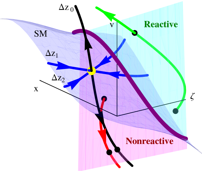
Figure 1: Geometric objects in phase space for Eqns. (3) with an anharmonic barrier. The TS trajectory is indicated by a yellow dot. Its stable manifold (SM, light blue surface and trajectories therein) and its unstable manifold (black curve) move and get deformed randomly. The purple curve marks the intersection of the SM with the surface of initial conditions (plane $x=0$). It partitions the surface of initial conditions into reactive (green) and nonreactive (red) regions and defines the critical velocity $V^{\ddagger}(\zeta)$. Representative reactive (green) and nonreactive (red) trajectories intersect the surface of initial conditions as indicated by black dots.

Method

For the sake of a simple presentation we restrict ourselves to systems with one degree of freedom (dof), although the generalization to higher dimensions is straightforward. It will be reported elsewhere Bartsch et al. (2015).

The reduced dynamics of a 1-dof system coupled to an external heat bath with memory effects can be adequately described by the GLE Zwanzig (2001)

$$m\ddot{x}=-\frac{dU(x)}{dx}-m\int_{-\infty}^{t}\gamma(t-s)\,\dot{x}(s)\,ds+mR_{\alpha}(t),$$ (1)

where $m$ is the mass of the particle, $x$ its position, $U$ the potential of mean force, $\gamma(t)$ the friction kernel, and $R_{\alpha}(t)$ the fluctuating colored noise force per unit mass exerted by the heat bath. It is related to $\gamma(t)$ by the fluctuation-dissipation theorem, $\left\langle R_{\alpha}(0)R_{\alpha}(t)\right\rangle_{\alpha}=k_{\text{B}}T\,\gamma(t)/m$, where $\left\langle...\right\rangle_{\alpha}$ denotes the average over the different realizations $\alpha$ of the noise.

If the friction kernel takes the exponential form

$$\gamma(t)=\frac{\gamma_{0}}{\tau}\,\exp(-t/\tau)$$ (2)

with a characteristic correlation time $\tau$ and a damping strengh $\gamma_{0}$, the GLE (1) can be replaced by a system of differential equations on a finite dimensional extended phase space Ferrario and Grigolini (1979); Grigolini (1982); Marchesoni and Grigolini (1983); Martens (2002)

$$\dot{x}=v,\;\dot{v}=\omega_{\text{b}}^{2}x+f(x)+\zeta,\;\dot{\zeta}=-\frac{\gamma_{0}}{\tau}\,v-\frac{1}{\tau}\,\zeta+\xi_{\alpha}(t),$$ (3)

where the mean force $-dU(x)/dx=m\omega_{\text{b}}^{2}x+mf(x)$ is split into a linear term and non-linear corrections $f(x)=-\varepsilon c_{3}x^{2}-\varepsilon^{2}c_{4}x^{3}-\dots$. The perturbation parameter $\varepsilon$ measures the anharmonicity of the barrier potential and will be set equal to 1 at the end of the calculation. The auxiliary coordinate $\zeta$ is given by $\zeta=-\int_{-\infty}^{t}\gamma(t-s)\,\dot{x}(s)\,ds$, and $\xi_{\alpha}$ is a white noise source satisfying the fluctuation–dissipation theorem $\left\langle\xi_{\alpha}(t)\;\xi_{\alpha}(s)\right\rangle_{\alpha}=[2k_{\text{B}}T\,\gamma_{0}/(m\tau^{2})]\delta(t-s)$.

If $f(x)=0$, the equations of motion (3) are linear and can be solved by diagonalizing the coefficient matrix. We find one positive eigenvalue $\lambda_{0}$ and two eigenvalues $\lambda_{1,2}$ that are negative or have negative real parts. The corresponding diagonal coordinates are denoted by $z_{i}$.

Equations (3) have a unique solution, called the TS trajectory Bartsch et al. (2005a, b); Kawai et al. (2007); Revuelta et al. (2012); Bartsch et al. (2012) that remains “jiggling” in the vicinity of the saddle point for all times. It depends on the realization $\alpha$ of the noise. We denote its diagonal coordinates by $z_{i}^{\ddagger}(t)$ and its position by $x^{\ddagger}(t)$. For the harmonic barrier, i.e. $f(x)=0$, the coordinates $z_{i}^{\ddagger}(t)$ can be obtained explicitly as an integral over the noise $\xi_{\alpha}$ Bartsch et al. (2005b); Revuelta et al. (2012); Bartsch et al. (2012). The TS trajectory gives rise to a time-dependent DS $x=x^{\ddagger}(t)$ that is recrossing-free in the harmonic approximation Bartsch et al. (2005a, b) as well as in anharmonic systems Craven et al. (2014a, b, 2015). However, we will not consider this DS any further and focus instead on the invariant structures that determine the reaction dynamics.

In relative coordinates $\Delta z_{i}=z_{i}-z_{i}^{\ddagger},$ Eq. (3) reads

$$\Delta\dot{z}_{i}=\lambda_{i}\,\Delta z_{i}+K_{i}\,f(x).$$ (4)

Here $K_{i}=-(\lambda_{j}+\lambda_{k})/[(\lambda_{i}-\lambda_{j})(\lambda_{i}-\lambda_{k})]$, where $i,j,k$ take the values $0,1,2$ and must be different. In the harmonic limit Eq. (4) has the simple solution $\Delta z_{i}(t)=\Delta z_{i}(0)\exp(\lambda_{i}t)$. Thus, as $\lambda_{0}>0$, $\Delta z_{0}(t)$ is associated with an exponentially growing unstable direction in phase space, whereas $\Delta z_{1}(t)$ and $\Delta z_{2}(t)$ are both associated with stable directions. The plane $\Delta z_{0}=0$ forms the SM of the TS trajectory. Trajectories within it asymptotically approach the TS trajectory as $t\to\infty$; they are trapped near the barrier top. Because the SM contains trajectories that are neither reactive nor nonreactive, it separates reactive from nonreactive trajectories.

When anharmonic terms are present, the SM is deformed in a time-dependent manner, but it stills remains the separatrix between reactive and nonreactive trajectories: All trajectories starting above the SM approximate the unstable manifold for large positive values of $\Delta z_{0}$ and finish in the product well defined by $x>0$, while trajectories that lie below the SM will follow the negative part of the unstable manifold into the reactant well $x<0$, as sketched in Fig. 1.

Reaction rates

The reaction rate can be computed by sampling trajectories from a Boltzmann ensemble at the barrier top and calculating the reactive flux across the surface of initial conditions $x=0$. Under the TST assumption that this surface is recrossing free, i.e. a trajectory is reactive if it starts with an initial velocity $v>0$, this procedure yields a reaction rate $k^{\text{TST}}$ that overestimates the true rate $k^{\rm exact}$. The violation of the TST assumption can be quantified by the transmission factor $\kappa=k^{\rm exact}/k^{\text{TST}}\leq 1$. The exact rate is obtained if the flux calculation includes only trajectories that are actually reactive. These are the trajectories that lie above the SM, or, as Fig. 1 shows, whose initial velocity is larger than a critical velocity $V^{\ddagger}(\zeta)$ that depends on the realization of the noise and on the initial value of the auxiliary coordinate $\zeta$. This critical velocity encodes all the relevant information about the reaction dynamics. Because it leads to an exact characterization of reactive trajectories, the critical velocity and the SM that determines it are more fundamental to the theory than the DS that has customarily been used. We compute the critical velocity by a perturbative expansion $V^{\ddagger}=V^{{\ddagger}(0)}+\varepsilon V^{{\ddagger}(1)}+\varepsilon^{2}V^{{\ddagger}(2)}+\dots$. This computation follows the method developed in Refs. Revuelta et al., 2012; Bartsch et al., 2012 for the case of Markovian friction. Full details will be presented elsewhere Bartsch et al. (2015).

Equipped with the critical velocity one can compute Bartsch et al. (2008); Revuelta et al. (2012); Bartsch et al. (2012) the transmission factor $\kappa=\left\langle e^{-V^{{\ddagger}\,2}/2k_{\text{B}}T}\right\rangle_{\alpha,\zeta}$, which is averaged both over the noise $\alpha$ and the initial value of $\zeta$. Now, by expanding $\kappa$ as $\kappa=\kappa_{0}+\varepsilon\kappa_{1}+\varepsilon^{2}\kappa_{2}+\ldots$, we finally obtain its lowest order

$$\kappa_{0}=\frac{\lambda_{0}}{\omega_{\text{b}}},\qquad\kappa_{1}=0,$$

$$\kappa_{2} =-\frac{3\kappa_{0}k_{\text{B}}T}{4m\omega_{\text{b}}^{4}}\left(\frac{f^{0,0}_{0,1,-1}}{f^{0,0}_{1,\eta-1,\eta}}\right)^{2}\!\!\!\bigg{\{}\frac{2c_{3}^{2}\left[f^{2,4}_{110,329,-12}+5f^{10,0}_{4,-17,4}+2\left(f^{0,5}_{10,41,10}+f^{4,3}_{115,197,-28}+f^{6,2}_{115,22,8}+f^{8,1}_{55,-94,6}\right)\right]}{9\,\omega_{\text{b}}^{2}\,f^{0,0}_{0,1,\eta}\,f^{0,0}_{1,2\left(\eta-2\right),4\eta}f^{0,0}_{4,2\eta-1,\eta}}+c_{4}f^{0,0}_{0,1,\eta}\bigg{\}},$$ (5)

with $\eta=\lambda_{0}(1+\lambda_{0}\tau)/(\omega_{\text{b}}^{2}\,\tau)$, and $f^{a,b}_{c,d,e}=\kappa_{0}^{a}\,\eta^{b}\left(c\,\kappa_{0}^{4}+d\,\kappa_{0}^{2}+e\,\right)$. The leading order $\kappa_{0}$ recovers the well known Grote–Hynes theory (GHT) Grote and Hynes (1980). Because all odd order terms are zero, the perturbation expansion proceeds in powers of $k_{\text{B}}T$.

Model

To illustrate the performance of our method we apply it to a simple, yet realistic, model for the LiNC$\rightleftharpoons$LiCN isomerization. It has a number of properties that make it very attractive for dynamical studies. Most importantly, the bending mode in this system is very floppy, so that chaos sets in at moderate values of the excitation energy. This reaction has been extensively studied by some of us in the past and very recently in connection to THz reactivity control Pellouchoud and Reed (2015). Most relevant in the present context, it furnished the first observation García-Müller et al. (2008); Garcia-Muller et al. (2012) of the turnover predicted by Kramers in his 1940 seminal paper Kramers (1940); Pollak et al. (1989); Pollak and Ankerhold (2013).

To describe the configuration of the LiCN molecule, we use the distance $r$ between the C and N atoms, the distance $R$ of the Li atom from the center of mass of the CN fragment and the angle $\vartheta$ between the Li atom and the CN axis (see Fig. 2). Because the CN triple bond is very rigid, the distance $r$ will not deviate much from its equilibrium value $r_{e}=2.186\ \text{a.u.}$ A potential energy function describing the motion of the Li atom relative to a rigid CN was introduced by Essers et al. Esser et al. (1982). An improved model can be obtained by combining this potential with a Morse potential for the CN vibration Garcia-Muller et al. (2014). The potential energy of the molecule with $r=r_{e}$ is shown in the inset to Fig. 2. It has two wells at $\vartheta=0$ and $\vartheta=\pi$ rad that correspond to the two linear isomers Li–CN and Li–NC.

Extensive molecular dynamics (MD) simulations of this molecule in a bath of 512 argon atoms were reported in Refs García-Müller et al. (2008); Garcia-Muller et al. (2012). It was found there that the isomerization rates for the transitions from the Li–NC to Li–CN configuration and back can be well described by a one-dimensional model in which the molecule is assumed to move along the minimum energy path (MEP). The MEP and the corresponding potential energy profile are shown in Fig. 2. This effective potential yields the parameters in Table 1 that will be used in perturbation theory.

In our study, the dynamics is modeled by the GLE (1), in which the angle $\vartheta$ plays the role of the position $x$ and the potential $U$ is the MEP potential $U_{\text{MEP}}$ of Fig. 2. The mass $m$ is replaced by the moment of inertia $I_{\vartheta}$ that describes the rotation of the Li atom relative to the CN fragment. Though the value of $I_{\vartheta}$ varies along the MEP, in the spirit of TST it is fixed to its value at the saddle point of the potential, $I_{\vartheta}=42\,852\ \text{a.u.}$ The friction kernel is well approximated by the exponential form (2) with the decay time $\tau=0.84\gamma_{0}/\omega_{b}^{2}$ Garcia-Muller et al. (2014).

Table 1: Parameters of the effective potential shown in Fig. 2 for the two well minima (isomers) and the saddle point.

Parameter	Li–CN	Saddle point	Li–NC
$\vartheta$ (rad)	0	0.917	$\pi$
$U_{\text{MEP}}$ ($10^{-2}$ a.u.)	1.04	1.58	0
$\omega$ ($10^{-4}$ a.u.)	7.92	9.65	5.90
$c_{3}$ ($10^{-7}$ a.u.)	–	-8.0	–
$c_{4}$ ($10^{-7}$ a.u.)	–	7.4	–

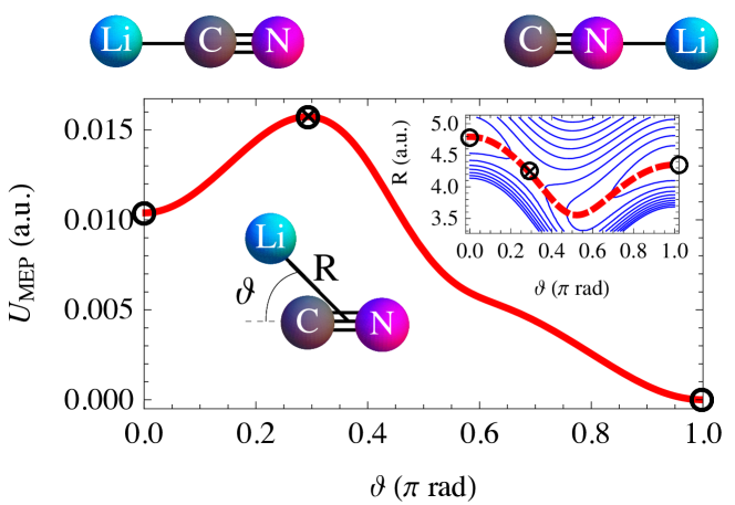
Figure 2: Effective potential for the one-dimensional model of LiCN isomerization. It corresponds to the minimum energy path connecting the two potential wells of the LiNC/LiCN molecular system. The configurations at the barrier top (crossed circle), and of the two stable isomers associated with the well minima (open circles) are also shown. Inset: Contour plot of the 2-dof potential. The minimum energy path is plotted superimposed in dashed red line.

Results

In Fig. 3, our predictions from perturbation theory (PT) for both the forward LiNC$\rightarrow$LiCN (top), and backward LiCN$\rightarrow$LiNC (bottom) reactions as a function of the adimensional friction $\gamma_{0}/\omega_{\text{b}}$ are compared with the results of all-atom MD simulations. Results are presented for temperatures $T$=2500K (blue), 3500K (green), and 5500K (red). Perturbative results in orders 0 and 2 are indicated by dashed and full lines, respectively. Because our rate theory, like GHT, is only valid in the spatial diffusion limit, where the friction has moderate to strong values, results for $\gamma_{0}/\omega_{b}<2$ are not included in Fig. 3. From the comparison, the following comments can be made.

The rates always increase with temperature, as should be expected for an activated process. The rates of the forward reaction are smaller than those of the backward reaction since the corresponding energy barrier is larger. The perturbative correction is negative. Its magnitude increases with temperature, as expected from Eq. (5). For the backward reaction, where the second-order correction is large, it provides a clear improvement of GHT for all values of the parameters. For the forward reaction, the second-order correction is barely noticeable at low temperatures. At the highest temperature $T=5500$K, where the perturbative correction is significant, the MD results are closer to GHT than to the PT results if damping is weak. For high damping, the second-order PT again provides a marked improvement over GHT.

In all cases, there is excellent agreement between the MD and PT rates. In fact, the agreement is striking, considering that the MD results were obtained from a simulation with an explicit argon bath that is much more complex than the simple one-dimensional model that yields the PT results.

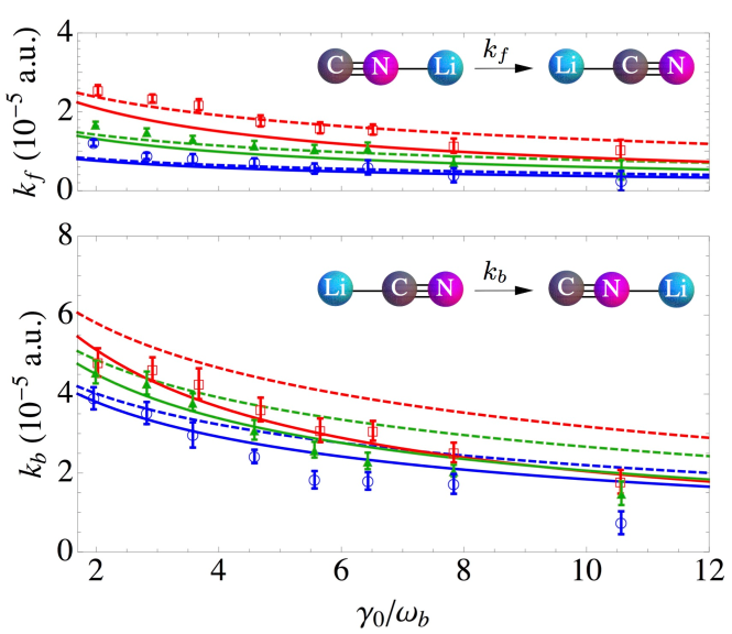
Figure 3: Reaction rates for the forward (top) and backward (bottom) LiNC$\rightleftharpoons$LiCN isomerization as a function of the bath friction. Perturbation theory results of order zero (dashed) and order two (solid) are shown for temperatures $T$=2500K (blue), 3500K (green), and 5500K (red). For comparison, results of all-atom MD simulations are shown by symbols with one-sigma error bars.

Concluding remarks

In summary, it is possible in principle to define a time-dependent recrossing–free DS in phase space for the dynamics of a particle in an anharmonic barrier that interacts with the environment via non–Markovian friction, i. e. via colored noise force. However, we have demonstrated that it is advantageous to base a rate calculation on invariant geometric structures, namely the SM of the TS trajectory, instead of a DS, as customary in TST. The SM allows the unambiguous identification of reactive trajectories simply by inspection of their initial conditions, without having to resort to any time–consuming numerical simulation. It provides a formally exact rate formula that we have evaluated through perturbation theory. In this way we have obtained an explicit expression for the transmission factor that corrects GHT by including anharmonic effects. It agrees well with the results of an all-atom model of LiCN isomerization in an argon bath. Finally, the method outlined here can be straightforwardly generalized to systems of higher dimensionality, as will be reported elsewhere Bartsch et al. (2015).

References

- Hänggi et al. (1990) P. Hänggi, P. Talkner, and M. Borkovec, Rev. Mod. Phys. 62, 251 (1990).
- Miller (1998) W. H. Miller, 110, 1 (1998), doi:10.1039/A805196H .
- Truhlar et al. (1996) D. G. Truhlar, B. C. Garrett, and S. J. Klippenstein, J. Phys. Chem. 100, 12771 (1996).
- Jaffé et al. (2002) C. Jaffé, S. D. Ross, M. W. Lo, J. Marsden, D. Farrelly, and T. Uzer, Phys. Rev. Lett. 89, 011101 (2002).
- Jaffé et al. (1999) C. Jaffé, D. Farrelly, and T. Uzer, Phys. Rev. A 60, 3833 (1999), doi:10.1103/PhysRevA.60.3833 .
- Miret-Artés and Pollak (2012) S. Miret-Artés and E. Pollak, Surface Science Reports 67, 161 (2012).
- Wanasundara et al. (2014) S. N. Wanasundara, R. J. Spiteri, and R. K. Bowles, J. Chem. Phys. 140, 024505 (2014).
- Garrett and Truhlar (2005) B. C. Garrett and D. G. Truhlar, in Theory and Applications of Computational Chemistry: The First Forty Years, edited by C. E. Dykstra, G. Frenking, K. S. Kim, and G. E. Scuseria (Elsevier, 2005) Chap. 5, pp. 67–87.
- Uzer et al. (2002) T. Uzer, C. Jaffé, J. Palacián, P. Yanguas, and S. Wiggins, Nonlinearity 15, 957 (2002).
- Waalkens et al. (2004a) H. Waalkens, A. Burbanks, and S. Wiggins, J. Phys. A 37, L257 (2004a).
- Waalkens et al. (2004b) H. Waalkens, A. Burbanks, and S. Wiggins, J. Chem. Phys. 121, 6207 (2004b).
- Bartsch et al. (2005a) T. Bartsch, R. Hernandez, and T. Uzer, Phys. Rev. Lett. 95, 058301 (2005a).
- Bartsch et al. (2005b) T. Bartsch, T. Uzer, and R. Hernandez, J. Chem. Phys. 123, 204102 (2005b).
- Bartsch et al. (2006) T. Bartsch, T. Uzer, J. M. Moix, and R. Hernandez, J. Chem. Phys. 124, 244310 (2006).
- Bartsch et al. (2008) T. Bartsch, T. Uzer, J. M. Moix, and R. Hernandez, J. Phys. Chem. B 112, 206 (2008).
- Craven et al. (2014a) G. T. Craven, T. Bartsch, and R. Hernandez, Phys. Rev. E 89, 040801(R) (2014a).
- Craven et al. (2014b) G. T. Craven, T. Bartsch, and R. Hernandez, J. Chem. Phys. 141, 041106 (2014b), 10.1063/1.4891471.
- Craven et al. (2015) G. T. Craven, T. Bartsch, and R. Hernandez, J. Chem. Phys. 142, 074108 (2015).
- Melnikov (1993) V. I. Melnikov, Phys. Rev. E 48, 3271 (1993).
- Kawai et al. (2007) S. Kawai, A. D. Bandrauk, C. Jaffé, T. Bartsch, J. Palacián, and T. Uzer, J. Chem. Phys. 126, 164306 (2007).
- Revuelta et al. (2012) F. Revuelta, T. Bartsch, R. M. Benito, and F. Borondo, J. Chem. Phys. 136, 091102 (2012).
- Bartsch et al. (2012) T. Bartsch, F. Revuelta, R. M. Benito, and F. Borondo, J. Chem. Phys. 136, 224510 (2012).
- Mullen et al. (2014) R. G. Mullen, J.-E. Shea, and B. Peters, J. Chem. Phys. 140, 041104 (2014).
- Pollak et al. (1989) E. Pollak, H. Grabert, and P. Hänggi, J. Chem. Phys. 91, 4073 (1989).
- García-Müller et al. (2008) P. L. García-Müller, F. Borondo, R. Hernandez, and R. M. Benito, Phys. Rev. Lett. 101, 178302 (2008).
- Pollak and Ankerhold (2013) E. Pollak and J. Ankerhold, J. Chem. Phys. 138 (2013), 10.1063/1.4802010.
- Pollak and Talkner (1993) E. Pollak and P. Talkner, Phys. Rev. E 47, 922 (1993).
- Ianconescu and Pollak (2015) R. Ianconescu and E. Pollak, J. Chem. Phys. 143, 104104 (2015).
- Zwanzig (2001) R. Zwanzig, Nonequilibrium Statistical Mechanics (Oxford University Press, London, 2001).
- Bartsch et al. (2015) T. Bartsch, F. Revuelta, R. M. Benito, and F. Borondo, in preparation (2015).
- Ferrario and Grigolini (1979) M. Ferrario and P. Grigolini, J. Math. Phys. 20, 2567 (1979).
- Grigolini (1982) P. Grigolini, Journal of Statistical Physics 27, 283 (1982).
- Marchesoni and Grigolini (1983) F. Marchesoni and P. Grigolini, J. Chem. Phys. 78, 6287 (1983).
- Martens (2002) C. C. Martens, J. Chem. Phys. 116, 2516 (2002).
- Grote and Hynes (1980) R. F. Grote and J. T. Hynes, J. Chem. Phys. 73, 2715 (1980).
- Pellouchoud and Reed (2015) L. A. Pellouchoud and E. J. Reed, Phys. Rev. A 91, 052706 (2015).
- Garcia-Muller et al. (2012) P. L. Garcia-Muller, R. Hernandez, R. M. Benito, and F. Borondo, J. Chem. Phys. 137, 204301 (2012).
- Kramers (1940) H. A. Kramers, Physica (Utrecht) 7, 284 (1940).
- Esser et al. (1982) R. Esser, J. Tennyson, and P. E. S. Wormer, Chem. Phys. Lett. 108, 223 (1982).
- Garcia-Muller et al. (2014) P. L. Garcia-Muller, R. Hernandez, R. M. Benito, and F. Borondo, J. Chem. Phys. 141, 074312 (2014).