On Classical and Bayesian Asymptotics in Stochastic Differential Equations with Random Effects having Mixture Normal Distributions

Abstract

Delattre et al. (2013) considered a system of stochastic differential equations ($SDE$s) in a random effects setup. Under the independent and identical ($iid$) situation, and assuming normal distribution of the random effects, they established weak consistency of the maximum likelihood estimators ($MLE$s) of the population parameters of the random effects.

In this article, respecting the increasing importance and versatility of normal mixtures and their ability to approximate any standard distribution, we consider the random effects having mixture of normal distributions and prove asymptotic results associated with the $MLE$s in both independent and identical ($iid$) and independent but not identical (non-$iid$) situations. Besides, we consider $iid$ and non-$iid$ setups under the Bayesian paradigm and establish posterior consistency and asymptotic normality of the posterior distribution of the population parameters, even when the number of mixture components is unknown and treated as a random variable.

Although ours is an independent work, we later noted that Delattre et al. (2016) also assumed the $SDE$ setup with normal mixture distribution of the random effect parameters but considered only the $iid$ case and proved only weak consistency of the $MLE$ under an extra, strong assumption as opposed to strong consistency that we are able to prove without the extra assumption. Furthermore, they did not deal with asymptotic normality of $MLE$ or the Bayesian asymptotics counterpart which we investigate in details.

Ample simulation experiments and application to a real, stock market data set reveal the importance and usefulness of our methods even for small samples.
Keywords: Asymptotic normality; Finite mixture of normals; Maximum likelihood estimator; Posterior consistency; Random effects; Stochastic differential equations.

1 Introduction

Data pertaining to inter-individual variability and intra-individual variability with respect to continuous time can be modeled through systems of stochastic differential equations ($SDE$s) consisting of random effects. In this regard, Delattre et al. (2013), Maitra and Bhattacharya (2015), Maitra and Bhattacharya (2016) investigate asymptotic inference in the context of systems of $SDE$s of the following form:

$$dX_{i}(t)=\phi_{i}b(X_{i}(t))dt+\sigma(X_{i}(t))dW_{i}(t),\quad\mbox{with}\quad X_{i}(0)=x^{i},~{}i=1,\ldots,n,$$ (1.1)

where, for $i=1,\ldots,n$, the stochastic process $X_{i}(t)$ is assumed to be continuously observed on the time interval $[0,T_{i}]$ with $T_{i}>0$ known, and corresponding to the $i$-th process initial values $\{x^{i};~{}i=1,\ldots,n\}$ are also assumed to be known. Here $\{\phi_{i};~{}i=1,\ldots,n\}$ are random effect parameters independent of the Brownian motions $\{W_{i}(\cdot);~{}i=1,\ldots,n\}$. The above authors assume that $\phi_{i}$ are independently and identically distributed ($iid$) with common distribution $g(\varphi,\theta)d\nu(\varphi)$ where $g(\varphi,\theta)$ is a density with respect to a dominating measure $\nu$ on $\mathbb{R}^{d}$ for all $\theta$ ($\mathbb{R}$ is the real line and $d$ is the dimension). Here the unknown parameter to be estimated is $\theta\in\Omega\subset\mathbb{R}^{p}$ ($p\geq 2d$). In particular, the above authors assume that $g(\varphi,\theta)$ is the Gaussian density with unknown means and covariance matrix, which are to be learned from the data and the model for classical inference (see Delattre et al. (2013), Maitra and Bhattacharya (2016)), and from a combination of the data, model and the prior for Bayesian inference (see Maitra and Bhattacharya (2015)). Statistically, the $i$-th process $X_{i}(\cdot)$ corresponds to the $i$-th individual and the corresponding random effect is $\phi_{i}$. The following conditions (see Delattre et al. (2013), Maitra and Bhattacharya (2015) and Maitra and Bhattacharya (2016)) that we assume ensure existence of solutions of (1.1):

• 1. $b(\cdot)$ and $\sigma(\cdot)$ are $C^{1}$ (differentiable with continuous first derivative) on $\mathbb{R}$ satisfying $b^{2}(x)\leq K(1+x^{2})$ and $\sigma^{2}(x)\leq K(1+x^{2})$ for all $x\in\mathbb{R}$, for some $K>0$.

  2. Almost surely for each $i\geq 1$,

     $$\int_{0}^{T_{i}}\frac{b^{2}(X_{i}(s))}{\sigma^{2}(X_{i}(s))}ds<\infty.$$

Delattre et al. (2013) show that the likelihood, depending upon $\theta$, admits a relatively simple form involving the following sufficient statistics:

$$U_{i}=\int_{0}^{T_{i}}\frac{b(X_{i}(s))}{\sigma^{2}(X_{i}(s))}dX_{i}(s),\quad V_{i}=\int_{0}^{T_{i}}\frac{b^{2}(X_{i}(s))}{\sigma^{2}(X_{i}(s))}ds,\quad i=1,\ldots,n.$$ (1.2)

The exact likelihood is given by

$$L(\theta)=\prod_{i=1}^{n}\lambda_{i}(X_{i},\theta),$$ (1.3)

where

$$\lambda_{i}(X_{i},\theta)=\int_{\mathbb{R}}g(\varphi,\theta)\exp\left(\varphi U_{i}-\frac{\varphi^{2}}{2}V_{i}\right)d\nu(\varphi).$$ (1.4)

For the Gaussian distribution of $\phi_{i}$ with mean $\mu$ and variance $\omega^{2}$, that is, with $g(\varphi,\theta)d\nu(\varphi)\equiv N\left(\mu,\omega^{2}\right)$, it is easy to obtain the following form of $\lambda_{i}(X_{i},\theta)$ (see Delattre et al. (2013)):

$$\lambda_{i}(X_{i},\theta)=\frac{1}{\left(1+\omega^{2}V_{i}\right)^{1/2}}\exp\left[-\frac{V_{i}}{2\left(1+\omega^{2}V_{i}\right)}\left(\mu-\frac{U_{i}}{V_{i}}\right)^{2}\right]\exp\left(\frac{U^{2}_{i}}{2V_{i}}\right),$$ (1.5)

where $\theta=(\mu,\omega^{2})\in\Omega\subset\mathbb{R}\times\mathbb{R}^{+}$. As in Delattre et al. (2013), Maitra and Bhattacharya (2016) and Maitra and Bhattacharya (2015) here also we assume that

• $\Omega$ is compact.

Delattre et al. (2013) consider $x^{i}=x$ and $T_{i}=T$ for $i=1,\ldots,n$, so that the setup boils down to the $iid$ situation, and investigate asymptotic properties of the $MLE$ of $\theta$, providing proofs of consistency and asymptotic normality. As an alternative, Maitra and Bhattacharya (2016) verify the regularity conditions of existing results in general setups provided in Schervish (1995) and Hoadley (1971) to prove asymptotic properties of the $MLE$ in this $SDE$ setup in both $iid$ and non-$iid$ cases. Here, by the non-$iid$ setup, we mean that the processes $X_{i}(\cdot)$ are independent, but not identical, which ensues when we allow for unequal initial values $x^{i}$ and unequal time points $T_{i}$.

Interestingly, the alternative way of verification of existing general results allowed Maitra and Bhattacharya (2016) to come up with stronger results under weaker assumptions, compared to Delattre et al. (2013).

Maitra and Bhattacharya (2015), for the first time in the literature, established Bayesian asymptotic results $SDE$-based random effects model, for both $iid$ and non-$iid$ setups. Specifically, considering prior distributions $\pi(\theta)$ of $\theta$, they established asymptotic properties of the corresponding posterior

$$\pi_{n}(\theta|X_{1},\ldots,X_{n})=\frac{\pi(\theta)\prod_{i=1}^{n}\lambda_{i}(X_{i}|\theta)}{\int_{\psi\in\Omega}\pi(\psi)\prod_{i=1}^{n}\lambda_{i}(X_{i}|\psi)d\psi}$$ (1.6)

as the sample size $n$ tends to infinity, through the verification of regularity conditions existing in Choi and Schervish (2007) and Schervish (1995).

In this article, we extend the asymptotic works of Maitra and Bhattacharya (2016) and Maitra and Bhattacharya (2015) assuming that the random effects are modeled by mixtures of normal distributions. The importance and generality of such mixture models are briefly discussed in Section 1.1.

1.1 Need for mixture distribution for the random effects parameters

The need for validation of our asymptotic results established in Maitra and Bhattacharya (2016) and Maitra and Bhattacharya (2015) for a bigger class of distributions corresponding to the random effect parameter $\phi$ leads us to consider mixture of normal distributions as the distribution of $\phi$, since any continuous density can be approximated arbitrarily accurately by an appropriate normal mixture.

Indeed, as is well-known, the unknown data generating process can be flexibly modeled by a mixture of parametric distributions. In fact, when a single parametric family can not provide a satisfactory model due to local variations in the observed data, mixture models can handle quite complex distributions by the appropriate choice of its components. So mixture distributions can be thought as the basis approximation to the unknown distributions. That mixture of normals with enough components can approximate any multivariate density, is established by Norets and Pelenis (2012). For instance, Theorems 1–3 of their article show under mild conditions that when the number of mixture components $M$ is fixed, for a given $\epsilon>0$ there exists $M$ such that the $L_{1}$ distance between the predictive density and the data generating process density is less than $\epsilon$ almost surely.

As infinite degree of smoothness and wide range of flexibility of mixture of normal densities allow us to model any unknown smooth density, it has been used for various inference problems including cluster analysis, density estimation, and robust estimation (see, for example, Banfield and Raftery (1993), Lindsay (1995), Roeder and Wasserman (1997)). Mixture models have also been adopted in hazards models (Louzada-Neto et al. (2002)), structural equation models (Zhu and Lee (2001)), analysis of proportions (Brooks (2001)), disease mapping (Green and Richardson (2002)), neural networks (Bishop (1995)), and in many more areas. Wirjanto and Xu (2009) provide a survey on recent developments and applications of normal mixture models in empirical finance.

Apart from the applicabilities of mixture models to various well-known statistical problems, it is worth noting that mixtures have important roles to play even in random effects models. Indeed, since mixture models are appropriate for data that are expected to arise from different sub-populations, these provide interesting extension of ordinary random effects models to random effects models associated with multiple sub-populations. From the authors’ perspective, this provides a particularly sound motivation for considering mixture distributions for the random effects.

It is important to note that while we independently pursued our investigation on system of $SDE$s where the random effect parameters are samples from Gaussian mixtures, we later came to know that it has also been considered by Delattre et al. (2016). However, asymptotically, their contribution is confined to only proving weak consistency of the $MLE$ in the $iid$ setup. In contrast, we are able to prove strong and weak consistency of the $MLE$ in the $iid$ and non-$iid$ cases, respectively, asymptotic normality of the $MLE$ in both $iid$ and non-$iid$ setups, and consistency and asymptotic normality of the Bayesian posterior distribution.

For finite samples Delattre et al. (2016) recommend the standard $EM$ algorithm (Dempster et al. (1977)) for computation of $MLE$ and the standard Bayes Information Criterion ($BIC$) (see, for example, Kass and Raftery (1995)) for selecting the number of mixture components (see Leroux (1992) and Keribin (2000) for $BIC$ related to mixture models). In the Bayesian setup it is natural to consider the number of mixture components to be unknown and place a prior on this unknown quantity. This of course renders the problem variable-dimensional. We develop the Bayesian asymptotic theory for this variable-dimensional setup as well.

Bayesian model implementation in the variable-dimensional framework is a non-trivial exercise and it is now well-known that the traditional reversible jump Markov Chain Monte Carlo method (Green (1995), Richardson and Green (1997)) can be quite inefficient for the purpose. Recently, Das and Bhattacharya (2019) have proposed a novel and efficient transformation based variable-dimensional Markov chain Monte Carlo method to simulate from variable-dimensional distributions; they refer to this method as Transdimensional Transformation based Markov chain Monte Carlo (TTMCMC) and demonstrate in particular the success of this method in mixture problems with unknown number of components. Indeed, as we demonstrate in this article with simulation studies and a real stock market data application, even in the $SDE$ setup, TTMCMC yields excellent performance.

There is another issue to be remarked about, namely, the well-known label-switching problem associated with mixtures, which is also persistent in our $SDE$ setup. Indeed, as is evident from (2.1) and (2.2), the likelihood remains the same even if the labels of $\left\{(a_{k},\beta_{k}):~{}k=1,\ldots,M\right\}$ are permuted, showing non-identifiability of the likelihood with respect to label-switching of the parameter components. Under somewhat restrictive assumption (see (H4) of Delattre et al. (2016)), Delattre et al. (2016) show that if two such $SDE$ mixtures with two sets of parameters are the same, then the two sets of parameters are also the same. However, that simply does not even touch the label-switching problem, and the weak consistency of $MLE$ proved by Delattre et al. (2016) in the $iid$ setup holds up to label-switching. In contrast, none of our results require assumption (H4) of Delattre et al. (2016), which are still unique up to label-switching. Specifically, in the $iid$ case we have been able to prove strong consistency of the $MLE$ under weaker assumption compared to weak consistency proved by Delattre et al. (2016) under stronger assumption.

The rest of our paper is structured as follows. In Section 2 we describe the likelihood corresponding to normal mixture distribution of the random effects, and in Sections 3 and 4 we investigate asymptotic properties of $MLE$ in the $iid$ and non-$iid$ contexts, respectively. In Sections 5 and 6 we investigate Bayesian asymptotics in the $iid$ and non-$iid$ setups, respectively. In Section 7 we address the Bayesian asymptotic theory when the number of mixture components is unknown and considered random. Brief discussions on the validity of our asymptotic theory for non-multiplicative and multidimensional linear random effects are provided in Sections S-3 and S-4, respectively, of the supplement, whose sections and figures have the prefix “S-” when referred to in this paper. In Section 8 we provide a brief overview of our simulation studies, conducted in nine separate cases. The complete details of the simulation experiments, illustrating the usefulness of our Bayesian methodology with TTMCMC implementation, are presented in Section S-5 of the supplement. In Section 9 we consider application to a real stock market data set. We summarize our work and provide concluding remarks in Section 10. Additional technical details are provided in the supplement.

Notationally, “$\stackrel{{\scriptstyle a.s.}}{{\rightarrow}}$”, “$\stackrel{{\scriptstyle P}}{{\rightarrow}}$” and “$\stackrel{{\scriptstyle\mathcal{L}}}{{\rightarrow}}$” denote convergence “almost surely”, “in probability” and “in distribution”, respectively.

2 Likelihood with respect to normal mixture distribution of the random effects

We consider the following normal mixture form of the distribution of $\phi$:

$$g(\varphi,\theta)d\nu(\varphi)\equiv\sum_{k=1}^{M}a_{k}N(\mu_{k},\omega_{k}^{2}),$$

such that $a_{k}\geq 0$ for $k=1,\ldots,M$ and $\sum_{k=1}^{M}a_{k}=1$. We assume that $\theta=(\gamma,\beta)$ where $\gamma=(a_{1},a_{2},\ldots,a_{M})$ and $\beta=(\beta_{1},\ldots,\beta_{M})$, such that $\beta_{i}=(\mu_{i},\omega_{i}^{2})$; $i=1,\ldots,M$. Here, for all $k=1,\ldots,M$, $(\mu_{k},\omega^{2}_{k})\in\Omega_{\beta}\subset\mathbb{R}\times\mathbb{R}^{+}$. We assume that $\Omega_{\beta}$ is compact, so that, denoting the simplex by the compact space $\Omega_{\gamma}$ on which $\gamma$ lie, it follows that $\Omega=\Omega_{\gamma}\times\Omega_{\beta}$ is compact, in accordance with (H2). Our likelihood corresponding to the $i$-th individual is

$$\lambda_{i}(X_{i},\theta)=\sum_{k=1}^{M}a_{k}f(X_{i}|\beta_{k}),$$ (2.1)

where

$$f(X_{i}|\beta_{k})=\frac{1}{\left(1+\omega_{k}^{2}V_{i}\right)^{1/2}}\exp\left[-\frac{V_{i}}{2\left(1+\omega_{k}^{2}V_{i}\right)}\left(\mu_{k}-\frac{U_{i}}{V_{i}}\right)^{2}\right]\exp\left(\frac{U^{2}_{i}}{2V_{i}}\right).$$ (2.2)

Assuming independence of the individuals conditional on the parameters, it then follows that the complete likelihood is the product of (2.1) over the $n$ individuals, having the form (1.3).

Note that, due to non-identifiability of the mixture form of the subject-wise likelihood (2.1), our asymptotic results will be unique up to label switching (see, for example, Redner (1981)).

3 Consistency and asymptotic normality of $MLE$ in the $iid$ setup

3.1 Strong consistency of $MLE$

Consistency of the $MLE$ under the $iid$ setup can be verified through the verification of the regularity conditions of the following theorem (Theorems 7.49 and 7.54 of Schervish (1995)); for our purpose we present the version for compact $\Omega$.

Theorem 1 (Schervish (1995))

Let $\{X_{n}\}_{n=1}^{\infty}$ be conditionally $iid$ given $\theta$ with density $\lambda_{1}(x|\theta)$ with respect to a measure $\nu$ on a space $\left(\mathcal{X}^{1},\mathcal{B}^{1}\right)$. Fix $\theta_{0}\in\Omega$, and define, for each $S\subseteq\Omega$ and $x\in\mathcal{X}^{1}$,

$$Z(S,x)=\inf_{\psi\in S}\log\frac{\lambda_{1}(x|\theta_{0})}{\lambda_{1}(x|\psi)}.$$

Assume that for each $\theta\neq\theta_{0}$, there is an open set $N_{\theta}$ such that $\theta\in N_{\theta}$ and that $E_{\theta_{0}}Z(N_{\theta},X_{i})>-\infty$. Also assume that $\lambda_{1}(x|\cdot)$ is continuous at $\theta$ for every $\theta$, a.s. $[P_{\theta_{0}}]$. Then, if $\hat{\theta}_{n}$ is the $MLE$ of $\theta$ corresponding to $n$ observations, it holds that $\underset{n\rightarrow\infty}{\lim}~{}\hat{\theta}_{n}=\theta_{0}$, a.s. $[P_{\theta_{0}}]$.

3.1.1 Verification of strong consistency of $MLE$ in our $SDE$ setup

Let the true set of parameter be $\theta_{0}=(\gamma_{0},\beta_{0})$ where $\gamma_{0}=(a_{0,1},a_{0,2},\ldots,a_{0,M})$ and $\beta_{0}=(\beta_{0,1},\beta_{0,2},\ldots,\beta_{0,M})$, such that $\beta_{0,i}=(\mu_{0,i},\omega_{0,i}^{2})$ for $i=1,\ldots,M$.

To verify the conditions of Theorem 1 in our case, we note that for any $x$, $\lambda_{1}(x|\theta)=\sum_{k=1}^{M}a_{k}f(x|\beta_{k})$ where $f(x|\beta_{k})$ given by (2.2) is clearly continuous in $\beta_{k}$, implying continuity of $\lambda_{1}(x|\theta)$ in $\theta$. Also, it follows from the proof of Proposition 7 of Delattre et al. (2013) that

$$\log\frac{f(x|\beta_{k})}{f(x|\beta_{0,1})} =\frac{1}{2}\log\left(\frac{1+\omega_{0,1}^{2}V}{1+\omega^{2}_{k}V}\right)+\frac{1}{2}\frac{(\omega^{2}_{k}-\omega_{0,1}^{2})U^{2}}{(1+\omega_{0,1}^{2}V)(1+\omega^{2}_{k}V)}$$

$$\quad+\frac{\mu_{0,1}^{2}V}{2(1+\omega_{0,1}^{2}V)}-\frac{\mu_{0,1}U}{1+\omega_{0,1}^{2}V}-\left(\frac{\mu^{2}_{k}V}{2(1+\omega^{2}_{k}V)}-\frac{\mu_{k}U}{1+\omega^{2}_{k}V}\right)$$

$$\leq\frac{1}{2}\left\{\log\left(1+\frac{\omega_{0,1}^{2}}{\omega^{2}_{k}}\right)+\frac{|\omega_{0,1}^{2}-\omega^{2}_{k}|}{\omega_{0,1}^{2}}\right\}+\frac{1}{2}|\omega^{2}_{k}-\omega_{0,1}^{2}|\left(\frac{U}{1+\omega^{2}_{k}V}\right)^{2}\left(1+\frac{\omega^{2}_{k}}{\omega_{0,1}^{2}}\right)$$

$$\quad+|\mu_{0,1}|\left|\frac{U}{1+\omega^{2}_{k}V}\right|\left(1+\frac{|\omega^{2}_{k}-\omega_{0,1}^{2}|}{\omega_{0,1}^{2}}\right)+\left|\frac{\mu^{2}_{k}V}{2(1+\omega^{2}_{k}V)}\right|+\left|\frac{\mu_{k}U}{1+\omega^{2}_{k}V}\right|$$

$$\quad=C_{1}(U,V,\beta_{0,1},\beta_{k}),~{}\mbox{(say)}.$$ (3.1)

Hence,

$$f(x|\beta_{k})\leq\exp(C_{1}(U,V,\beta_{0,1},\beta_{k}))f(x|\beta_{0,1}).$$ (3.2)

Now, since $\log(x)=-\log\left(\frac{1}{x}\right)$, for $x>0$, we have

$$\log\frac{\lambda_{1}(x|\theta_{0})}{\lambda_{1}(x|\theta)} =-\log\left(\frac{\sum_{k=1}^{M}a_{k}f(x|\beta_{k})}{\sum_{k=1}^{M}a_{0,k}f(x|\beta_{0,k})}\right)$$

$$\geq-\log\left(\frac{\sum_{k=1}^{M}a_{k}f(x|\beta_{k})}{a_{0,1}f(x|\beta_{0,1})}\right)$$

$$\geq-\log\left(\frac{\sum_{k=1}^{M}a_{k}\exp(C_{1}(U,V,\beta_{0,1},\beta_{k}))f(x|\beta_{0,1}))}{a_{0,1}f(x|\beta_{0,1})}\right)\quad\mbox{(by (\ref{eq:relation_1}))}$$

$$\geq-\left|\log\left(\sum_{k=1}^{M}a_{k}\exp(C_{1}(U,V,\beta_{0,1},\beta_{k}))\right)\right|-\left|\log a_{0,1}\right|$$

$$\geq-\sum_{k=1}^{M}C_{1}(U,V,\beta_{0,1},\beta_{k})-|\log a_{0,1}|.$$ (3.3)

The last inequality is due to a result of Atienza et al. (2005), which we furnish below along with its proof:

Lemma 2

Atienza et al. (2005) $\sum_{k=1}^{M}a_{k}=1$, with $a_{k}\geq 0$ implies

$$\quad\left|\log\sum_{k=1}^{M}a_{k}f_{k}\right|\leq\sum_{k=1}^{M}|\log f_{k}|,$$

for $f_{k}>0$; $k=1,\ldots,M$.

Proof. Letting $\alpha=\min\{a_{k}:k=1,\ldots,M\}$ and $\beta=\max\{a_{k}:k=1,\ldots,M\}$, it follows that $\alpha\leq\sum_{k=1}^{M}a_{k}f_{k}\leq\beta$, which again leads to $\log\alpha\leq\log\left(\sum_{k=1}^{M}a_{k}f_{k}\right)\leq\log\beta$, by monotonicity of logarithm. Hence, $\left|\log\left(\sum_{k=1}^{M}a_{k}f_{k}\right)\right|\leq\max\{|\log\alpha|,|\log\beta|\}\leq\sum_{k=1}^{M}|\log f_{k}|$.   

Now taking $N_{\theta}$ to be any open subset of the relevant compact parameter space containing $\theta$, and noting that

$$E_{\theta_{0}}\left[\inf_{\theta\in N_{\theta}}\log\frac{\lambda_{1}(X|\theta_{0})}{\lambda_{1}(X|\theta)}\right]\geq-\sum_{k=1}^{M}\sup_{\theta\in N_{\theta}}C_{1}(U,V,\beta_{0,1},\beta_{k})-|\log a_{1}|,$$

it is sufficient to establish that $E_{\theta_{0}}\left[\underset{\theta\in N_{\theta}}{\sup}~{}C_{1}(U,V,\beta_{0,1},\beta_{k})\right]<+\infty$ for $k=1,\ldots,M$, in order to conclude that $E_{\theta_{0}}Z(N_{\theta},X_{i})>-\infty.$

Observation of the terms of $C_{1}(U,V,\beta_{0,1},\beta_{k})$ makes it clear that it is sufficient to show finiteness of $E_{\beta_{0,k}}\left(\frac{U}{1+\omega^{2}_{k}V}\right)^{2}$, $E_{\beta_{0,k}}\left|\frac{U}{1+\omega^{2}_{k}V}\right|$ and $E_{\beta_{0,k}}\left(\frac{V}{1+\omega^{2}_{k}V}\right)$.

Let us first prove finiteness of $E_{\beta_{0,k}}\left|\frac{U}{1+\omega^{2}_{k}V}\right|$. For $\omega^{2}_{k}>\omega^{2}_{0,k}$, note that

$$E_{\beta_{0,k}}\left|\frac{U}{1+\omega^{2}_{k}V}\right|=E_{\beta_{0,k}}\left(\frac{|U|}{1+\omega^{2}_{0,k}\left(\frac{\omega^{2}_{k}}{\omega^{2}_{0,k}}\right)V}\right)<E_{\beta_{0,k}}\left(\frac{|U|}{1+\omega^{2}_{0,k}V}\right)<\infty.$$

The last inequality holds due to Lemma 1 of Delattre et al. (2013). For $\omega^{2}_{k}<\omega^{2}_{0,k}$,

$$E_{\beta_{0,k}}\left|\frac{U}{1+\omega^{2}_{k}V}\right|=\left(\frac{\omega^{2}_{0,k}}{\omega^{2}_{k}}\right)E_{\beta_{0,k}}\left(\frac{|U|}{\left(\frac{\omega^{2}_{0,k}}{\omega^{2}_{k}}\right)+\omega^{2}_{0,k}V}\right)<\left(\frac{\omega^{2}_{0,k}}{\omega^{2}_{k}}\right)E_{\beta_{0,k}}\left(\frac{|U|}{1+\omega^{2}_{0,k}V}\right)<\infty.$$

In the same way, for $r\geq 1$,

$$E_{\beta_{0,k}}\left(\frac{|U|}{1+\omega^{2}_{k}V}\right)^{r}<\infty.$$ (3.4)

Also, since $\frac{V}{1+\omega^{2}_{k}V}<\frac{1}{\omega^{2}_{k}}$ almost surely, it follows that for $r\geq 1$,

$$E_{\beta_{0,k}}\left(\frac{V}{1+\omega^{2}_{k}V}\right)^{r}<\infty.$$ (3.5)

We have thus shown that $E_{\theta_{0}}Z(N_{\theta},X_{i})>-\infty$. Hence, $\hat{\theta}_{n}\stackrel{{\scriptstyle a.s.}}{{\rightarrow}}\theta_{0}$ $[P_{\theta_{0}}]$. We summarize the result in the form of the following theorem:

Theorem 3

Assume the $iid$ setup and conditions (H1) and (H2). Then the $MLE$ is strongly consistent in the sense that $\hat{\theta}_{n}\stackrel{{\scriptstyle a.s.}}{{\rightarrow}}\theta_{0}$  $[P_{\theta_{0}}]$.

The above theorem requires only a lower bound for $\log\frac{\lambda_{i}(X_{i}|\theta_{0})}{\lambda_{i}(X_{i}|\theta)}$ with finite expectation. But some of our later results will require existence of expectations of an upper bound for $\left|\log\frac{\lambda_{i}(X_{i}|\theta_{0})}{\lambda_{i}(X_{i}|\theta)}\right|$. We state and prove this result as Lemma 4.

Lemma 4

For any given $\theta\in\Omega$, $\left|\log\frac{\lambda_{i}(X_{i}|\theta_{0})}{\lambda_{i}(X_{i}|\theta)}\right|$ has an upper bound which has finite moments of all orders.

Proof. Since (3.3) provides a lower bound $\log\frac{\lambda_{i}(X_{i}|\theta_{0})}{\lambda_{i}(X_{i}|\theta)}$ with finite moments of all orders, let us now provide an upper bound for $\log\frac{\lambda_{i}(X_{i}|\theta_{0})}{\lambda_{i}(X_{i}|\theta)}$, which also has finite moments of all orders. Since

$$\log\frac{f(x|\beta_{0,k})}{f(x|\beta_{1})} =\frac{1}{2}\log\left(\frac{1+\omega_{1}^{2}V}{1+\omega^{2}_{0,k}V}\right)+\frac{1}{2}\frac{(\omega^{2}_{0,k}-\omega_{1}^{2})U^{2}}{(1+\omega_{1}^{2}V)(1+\omega^{2}_{0,k}V)}$$

$$\quad+\frac{\mu_{1}^{2}V}{2(1+\omega_{1}^{2}V)}-\frac{\mu_{1}U}{1+\omega_{1}^{2}V}-\left(\frac{\mu^{2}_{0,k}V}{2(1+\omega^{2}_{0,k}V)}-\frac{\mu_{0,k}U}{1+\omega^{2}_{0,k}V}\right)$$

$$\leq\frac{1}{2}\left\{\log\left(1+\frac{\omega_{1}^{2}}{\omega^{2}_{0,k}}\right)+\frac{|\omega_{1}^{2}-\omega^{2}_{0,k}|}{\omega_{1}^{2}}\right\}+\frac{1}{2}|\omega^{2}_{0,k}-\omega_{1}^{2}|\left(\frac{U}{1+\omega^{2}_{0,k}V}\right)^{2}\left(1+\frac{\omega^{2}_{0,k}}{\omega_{1}^{2}}\right)$$

$$\quad+|\mu_{1}|\left|\frac{U}{1+\omega^{2}_{0,k}V}\right|\left(1+\frac{|\omega^{2}_{0,k}-\omega_{1}^{2}|}{\omega_{1}^{2}}\right)+\left|\frac{\mu^{2}_{0,k}V}{2(1+\omega^{2}_{0,k}V)}\right|+\left|\frac{\mu_{0,k}U}{1+\omega^{2}_{0,k}V}\right|$$

$$\quad=C_{1}(U,V,\beta_{1},\beta_{0,k}),$$

it follows that

$$f(x|\beta_{0,k})\leq\exp(C_{1}(U,V,\beta_{1},\beta_{0,k}))f(x|\beta_{1}).$$ (3.6)

Now,

$$\log\frac{\lambda_{1}(x|\theta_{0})}{\lambda_{1}(x|\theta)} =\log\left(\frac{\sum_{k=1}^{M}a_{0,k}f(x|\beta_{0,k})}{\sum_{k=1}^{M}a_{k}f(x|\beta_{k})}\right)$$

$$\leq\log\left(\frac{\sum_{k=1}^{M}a_{0,k}f(x|\beta_{0,k})}{a_{1}f(x|\beta_{1})}\right)$$

$$\leq\left|\log\frac{\sum_{k=1}^{M}a_{0,k}\exp(C_{1}(U,V,\beta_{1},\beta_{0,k}))f(x|\beta_{1}))}{a_{1}f(x|\beta_{1})}\right|\quad\mbox{(by (\ref{eq:relation_1_2}))}$$

$$\leq\left|\log\sum_{k=1}^{M}a_{0,k}\exp(C_{1}(U,V,\beta_{1},\beta_{0,k}))\right|+|\log a_{1}|$$

$$=\sum_{k=1}^{M}C_{1}(U,V,\beta_{1},\beta_{0,k})+|\log a_{1}|\quad\mbox{(by Lemma \ref{lemma:atienza})}.$$ (3.7)

From (3.3) and (3.7) and existence of moments as shown in Delattre et al. (2013), as well as by the results (3.4) and (3.5), it follows that $\left|\log\frac{\lambda_{i}(X_{i}|\theta_{0})}{\lambda_{i}(X_{i}|\theta)}\right|$ has an upper bound which has finite moments of all orders under $\theta_{0}$, for any given $\theta\in\Omega$.   

3.2 Asymptotic normality of $MLE$

To verify asymptotic normality of $MLE$ we invoke the following theorem provided in Schervish (1995) (Theorem 7.63):

Theorem 5 (Schervish (1995))

Let $\Omega$ be a subset of $\mathbb{R}^{3M}$, and let $\{X_{n}\}_{n=1}^{\infty}$ be conditionally $iid$ given $\theta$ each with density $\lambda_{1}(\cdot|\theta)$. Let $\hat{\theta}_{n}$ be an $MLE$. Assume that $\hat{\theta}_{n}\stackrel{{\scriptstyle P}}{{\rightarrow}}\theta$ under $P_{\theta}$ for all $\theta$. Assume that $\lambda_{1}(x|\theta)$ has continuous second partial derivatives with respect to $\theta$ and that differentiation can be passed under the integral sign in the sense that $0=\frac{\partial}{\partial\theta_{j}}\int\lambda_{1}(x|\theta)d\nu(x)=\int\frac{\partial}{\partial\theta_{j}}\lambda_{1}(x|\theta)d\nu(x)$, for $j\geq 1$, where $\nu$ is the relevant dominating measure. Assume that there exists $H_{r}(x,\theta)$ such that, for each $\theta_{0}\in int(\Omega)$ and each $k,j$,

$$\sup_{\|\theta-\theta_{0}\|\leq r}\left|\frac{\partial^{2}}{\partial\theta_{k}\partial\theta_{j}}\log\lambda_{X_{1}|\Theta}(x|\theta_{0})-\frac{\partial^{2}}{\partial\theta_{k}\partial\theta_{j}}\log\lambda_{X_{1}|\Theta}(x|\theta)\right|\leq H_{r}(x,\theta_{0}),$$ (3.8)

with

$$\lim_{r\rightarrow 0}E_{\theta_{0}}H_{r}\left(X,\theta_{0}\right)=0.$$ (3.9)

Assume that the Fisher information matrix $\mathcal{I}(\theta)$ is finite and non-singular. Then, under $P_{\theta_{0}}$,

$$\sqrt{n}\left(\hat{\theta}_{n}-\theta_{0}\right)\stackrel{{\scriptstyle\mathcal{L}}}{{\rightarrow}}N\left(\boldsymbol{0},\mathcal{I}^{-1}(\theta_{0})\right).$$ (3.10)

3.2.1 Verification of the above regularity conditions for asymptotic normality in our $SDE$ setup

In Section 3.1.1 we proved almost sure consistency of the $MLE$ $\hat{\theta}_{n}$ in the $SDE$ setup. Hence, $\hat{\theta}_{n}\stackrel{{\scriptstyle P}}{{\rightarrow}}\theta$ under $P_{\theta}$ for all $\theta$.

We assume,

• For some real constant $K>0$,

  $$\frac{b^{2}(x)}{\sigma^{2}(x)}<K(1+x^{\tau}),\quad\mbox{for some}\quad\tau\geq 1$$

Note that (H3) implies moments of all orders of $V_{i}$ (given by 1.2) for all $i=1,\ldots,n$ are finite. Also note that, since for $k\geq 1$, $E[\phi_{i}]^{2k}<\infty$, for all $i=1,\ldots,n$, because of normal mixture distribution, Proposition 1 of Delattre et al. (2013) implies that for all $T>0,\underset{t\in[0,T]}{\sup}~{}E[X_{i}(t)]^{2k}<\infty$ for all $k\geq 1$ and $i=1,\ldots,n$.

That differentiation can be passed under the integral sign in our case, is proved in Section S-1 of the supplement. For the third order derivatives of $\log\lambda$ note that

$$\frac{\partial^{3}\log\lambda}{\partial\theta_{r}\partial\theta_{s}\partial\theta_{t}}=\frac{1}{\lambda}\frac{\partial^{3}\lambda}{\partial\theta_{r}\partial\theta_{s}\partial\theta_{t}}-\frac{1}{\lambda^{2}}\left[\frac{\partial^{2}\lambda}{\partial\theta_{r}\partial\theta_{s}}\frac{\partial\lambda}{\partial\theta_{t}}+\frac{\partial^{2}\lambda}{\partial\theta_{s}\partial\theta_{t}}\frac{\partial\lambda}{\partial\theta_{r}}+\frac{\partial^{2}\lambda}{\partial\theta_{t}\partial\theta_{r}}\frac{\partial\lambda}{\partial\theta_{s}}\right]+\frac{2}{\lambda^{3}}\frac{\partial\lambda}{\partial\theta_{r}}\frac{\partial\lambda}{\partial\theta_{s}}\frac{\partial\lambda}{\partial\theta_{t}}.$$ (3.11)

Denoting $\psi=(\mu_{1},\cdots,\mu_{M},\omega_{1}^{2},\cdots,\omega_{M}^{2}),$ the absolute values of the terms on the right hand side of the above equation are bounded by a sum of terms of the forms

$$\left|\frac{1}{\lambda}\frac{\partial^{3}f}{\partial\psi_{r}\partial\psi_{s}\partial\psi_{t}}\right|,\quad\left|\frac{1}{\lambda}\frac{\partial^{2}f}{\partial\psi_{r}\partial\psi_{s}}\right|,\quad\left|\frac{1}{\lambda}\frac{\partial f}{\partial\psi_{r}}\right|\quad\mbox{and}\quad\frac{f}{\lambda}.$$

That expectation of the upper bound of each term is finite, is proved in Section S-2 of the supplement, which implies that (3.8) and (3.9) clearly hold.

Now, following Delattre et al. (2013), Maitra and Bhattacharya (2016), Maitra and Bhattacharya (2015) we assume:

• The true value $\theta_{0}\in int\left(\Omega\right)$.

Now let us define $\mathcal{I}(\theta)$ to be the information matrix, whose $(r,s)$-th element is given by

$$\mathcal{I}_{rs}(\theta)=E_{\theta}\left[\frac{\partial\log\lambda}{\partial\theta_{r}}\frac{\partial\log\lambda}{\partial\theta_{s}}\right]=-E_{\theta}\left[\frac{\partial^{2}\log\lambda}{\partial\theta_{r}\partial\theta_{s}}\right]$$

That $\mathcal{I}(\theta)$ is well-defined is clear due to existence of derivatives up to the second order. Now, let $(b_{1},b_{2},\ldots,b_{M})$ be a real row vector where $\theta$ is $M$-dimensional. Then

$$E\left[b_{1}\frac{\partial\log\lambda}{\partial\theta_{1}}+b_{2}\frac{\partial\log\lambda}{\partial\theta_{2}}+\ldots+b_{M}\frac{\partial\log\lambda}{\partial\theta_{M}}\right]^{2}\geq 0$$

implying

$$\sum_{r=1}^{M}\sum_{s=1}^{M}b_{r}b_{s}\mathcal{I}_{rs}(\theta)\geq 0.$$

This shows that $\mathcal{I}(\theta)$ is positive semi-definite. We assume

• $\mathcal{I}(\theta_{0})$ is positive definite.

Hence, asymptotic normality of the $MLE$, of the form (3.10), holds in our case. Formally,

Theorem 6

Assume the $iid$ setup and conditions (H1) – (H5). Then the $MLE$ is asymptotically normally distributed as (3.10).

4 Consistency and asymptotic normality of $MLE$ in the non-$iid$ setup

In this section, as in Maitra and Bhattacharya (2016) and Maitra and Bhattacharya (2015) we allow $T_{i}\neq T$ and $x^{i}\neq x$ for each $1\leq i\leq n$. Consequently, here we deal with the setup where the processes $X_{i}(\cdot);~{}i=1,\ldots,n$, are independently, but not identically distributed. Following Maitra and Bhattacharya (2016) and Maitra and Bhattacharya (2015) we assume the following:

• The sequences $\{T_{1},T_{2},\ldots\}$ and $\{x^{1},x^{2},\ldots,\}$ are sequences in compact sets $\mathfrak{T}$ and $\mathfrak{X}$, respectively, so that there exist convergent subsequences with limits in $\mathfrak{T}$ and $\mathfrak{X}$. For notational convenience, we continue to denote the convergent subsequences as $\{T_{1},T_{2},\ldots\}$ and $\{x^{1},x^{2},\ldots\}$. Let us denote the limits by $T^{\infty}$ and $x^{\infty}$, where $T^{\infty}\in\mathfrak{T}$ and $x^{\infty}\in\mathfrak{X}$.

Following Maitra and Bhattacharya (2016) and Maitra and Bhattacharya (2015) we denote the process associated with the initial value $x$ and time point $t$ as $X(t,x)$, so that $X(t,x^{i})=X_{i}(t)$, and $X_{i}=\left\{X_{i}(t);~{}t\in[0,T_{i}]\right\}$. We also denote by $\phi(x)$ the random effect parameter associated with the initial value $x$ such that $\phi(x^{i})=\phi_{i}$. We assume

• $\phi(x)$ is a real-valued, continuous function of $x$, and that for $k\geq 1$, $\underset{x\in\mathfrak{X}}{\sup}~{}E\left[\phi(x)\right]^{2k}<\infty$.

As in Proposition 1 of Delattre et al. (2013), assumption (H7) implies that for any $T>0$,

$$\underset{t\in[0,T],x\in\mathfrak{X}}{\sup}~{}E\left[X(t,x)\right]^{2k}<\infty.$$ (4.1)

For $x\in\mathfrak{X}$ and $T\in\mathfrak{T}$, let

$$U(x,T) =\int_{0}^{T}\frac{b(X(s,x))}{\sigma^{2}(X(s,x))}dX(s,x);$$ (4.2)

$$V(x,T) =\int_{0}^{T}\frac{b^{2}(X(s,x))}{\sigma^{2}(X(s,x))}ds.$$ (4.3)

Clearly, $U(x^{i},T_{i})=U_{i}$ and $V(x^{i},T_{i})=V_{i}$, where $U_{i}$ and $V_{i}$ are given by (1.2).

Even in this non-$iid$ case (H3) ensures that moments of all orders of $V(x,T)$ are finite. Then, by Theorem 5 of Maitra and Bhattacharya (2016), the moments of uniformly integrable continuous functions of $U(x,T)$, $V(x,T)$ and $\theta$ are continuous in $x$, $T$ and $\theta$. In particular, the Kullback-Leibler distance and the information matrix, which we denote by $\mathcal{K}_{x,T}(\theta_{0},\theta)$ (or, $\mathcal{K}_{x,T}(\theta,\theta_{0})$) and $\mathcal{I}_{x,T}(\theta)$ respectively to emphasize dependence on the initial values $x$ and $T$, are continuous in $x$, $T$ and $\theta$. For $x=x^{k}$ and $T=T_{k}$, if we denote the Kullback-Leibler distance and the Fisher’s information as $\mathcal{K}_{k}(\theta_{0},\theta)$ ($\mathcal{K}_{k}(\theta,\theta_{0})$) and $\mathcal{I}_{k}(\theta)$, respectively, then continuity of $\mathcal{K}_{x,T}(\theta_{0},\theta)$ (or $\mathcal{K}_{x,T}(\theta,\theta_{0})$) and $\mathcal{I}_{x,T}(\theta_{0})$ with respect to $x$ and $T$ ensures that as $x^{k}\rightarrow x^{\infty}$ and $T_{k}\rightarrow T^{\infty}$, $\mathcal{K}_{x^{k},T_{k}}(\theta_{0},\theta)\rightarrow\mathcal{K}_{x^{\infty},T^{\infty}}(\theta_{0},\theta)=\mathcal{K}(\theta_{0},\theta)$, say. Similarly, $\mathcal{K}_{x^{k},T_{k}}(\theta,\theta_{0})\rightarrow\mathcal{K}(\theta,\theta_{0})$ and $\mathcal{I}_{x^{k},T_{k}}(\theta)\rightarrow\mathcal{I}_{x^{\infty},T^{\infty}}(\theta)=\mathcal{I}(\theta)$, say. Thanks to compactness, the limits $\mathcal{K}(\theta_{0},\theta)$, $\mathcal{K}(\theta,\theta_{0})$ and $\mathcal{I}(\theta)$ are well-defined Kullback-Leibler divergences and Fisher’s information, respectively. Consequently (see Maitra and Bhattacharya (2016), Maitra and Bhattacharya (2015)), the following hold for any $\theta\in\Omega$,

$$\underset{n\rightarrow\infty}{\lim}~{}\frac{\sum_{k=1}^{n}\mathcal{K}_{k}(\theta_{0},\theta)}{n} =\mathcal{K}(\theta_{0},\theta);$$ (4.4)

$$\underset{n\rightarrow\infty}{\lim}~{}\frac{\sum_{k=1}^{n}\mathcal{K}_{k}(\theta,\theta_{0})}{n} =\mathcal{K}(\theta,\theta_{0});$$ (4.5)

$$\underset{n\rightarrow\infty}{\lim}~{}\frac{\sum_{k=1}^{n}\mathcal{I}_{k}(\theta)}{n} =\mathcal{I}(\theta).$$ (4.6)

We assume that

• For any $\theta\in\Omega$, $\mathcal{I}(\theta)$ is positive definite.

4.1 Consistency of $MLE$ in the non-$iid$ setup

Following Hoadley (1971) we define the following:

$$R_{i}(\theta) =\log\frac{\lambda_{i}(X_{i}|\theta)}{\lambda_{i}(X_{i}|\theta_{0})}\quad\mbox{if}\ \ \lambda_{i}(X_{i}|\theta_{0})>0$$

$$=0\quad\quad\quad\quad\quad\quad\mbox{otherwise}.$$ (4.7)

$$R_{i}(\theta,\rho) =\sup\left\{R_{i}(\xi):\|\xi-\theta\|\leq\rho\right\}$$ (4.8)

$${\mathcal{V}}_{i}(r) =\sup\left\{R_{i}(\theta):\|\theta\|>r\right\}.$$ (4.9)

Following Hoadley (1971) we denote by $r_{i}(\theta)$, $r_{i}(\theta,\rho)$ and $v_{i}(r)$ to be expectations of $R_{i}(\theta)$, $R_{i}(\theta,\rho)$ and ${\mathcal{V}}_{i}(r)$ under $\theta_{0}$; for any sequence $\{A_{i};i=1,2,\ldots\}$ we denote $\sum_{i=1}^{n}A_{i}/n$ by $\bar{A}_{n}$.

Hoadley (1971) proved that if the following regularity conditions are satisfied, then the $MLE$ $\hat{\theta}_{n}\stackrel{{\scriptstyle P}}{{\rightarrow}}\theta_{0}$:

• $\Omega$ is a closed subset of $\mathbb{R}^{3M}$.

• $\lambda_{i}(X_{i}|\theta)$ is an upper semicontinuous function of $\theta$, uniformly in $i$, a.s. $[P_{\theta_{0}}]$.

• There exist $\rho^{*}=\rho^{*}(\theta)>0$, $r>0$ and $0<K^{*}<\infty$ for which

  1. $E_{\theta_{0}}\left[R_{i}(\theta,\rho)\right]^{2}\leq K^{*},\quad 0\leq\rho\leq\rho^{*}$;

  2. $E_{\theta_{0}}\left[{\mathcal{V}}_{i}(r)\right]^{2}\leq K^{*}$.

• 1. $\underset{n\rightarrow\infty}{\lim}~{}\bar{r}_{n}(\theta)<0,\quad\theta\neq\theta_{0}$;

  2. $\underset{n\rightarrow\infty}{\lim}~{}\bar{v}_{n}(r)<0$.

• $R_{i}(\theta,\rho)$ and ${\mathcal{V}}_{i}(r)$ are measurable functions of $X_{i}$.

Actually, conditions (3) and (4) can be weakened but these are more easily applicable (see Hoadley (1971) for details).

4.1.1 Verification of the regularity conditions

Since $\Omega$ is compact in our case, the first regularity condition clearly holds.

For the second regularity condition, note that given $X_{i}$, $\lambda_{i}(X_{i}|\theta)$ is continuous (as $\lambda_{i}(X_{i}|\theta)=\sum_{k=1}^{M}a_{k}f_{k}(X_{i}|\beta_{k})$ where each $f_{k}(X_{i}|\beta_{k})$ is continuous), in fact, uniformly continuous in $\theta$ in our case, since $\Omega$ is compact. Hence, for any given $\epsilon>0$, there exists $\delta_{i}(\epsilon)>0$, independent of $\theta$, such that $\|\theta_{1}-\theta_{2}\|<\delta_{i}(\epsilon)$ implies $\left|\lambda(X_{i}|\theta_{1})-\lambda(X_{i}|\theta_{2})\right|<\epsilon$. Now consider a strictly positive function $\delta_{x,T}(\epsilon)$, continuous in $x\in\mathfrak{X}$ and $T\in\mathfrak{T}$, such that $\delta_{x^{i},T_{i}}(\epsilon)=\delta_{i}(\epsilon)$. Let $\delta(\epsilon)=\underset{x\in\mathfrak{X},T\in\mathfrak{T}}{\inf}\delta_{x,T}(\epsilon)$. Since $\mathfrak{X}$ and $\mathfrak{T}$ are compact, it follows that $\delta(\epsilon)>0$. Now it holds that $\|\theta_{1}-\theta_{2}\|<\delta(\epsilon)$ implies $\left|\lambda(X_{i}|\theta_{1})-\lambda(X_{i}|\theta_{2})\right|<\epsilon$, for all $i$. Hence, the second regularity condition is satisfied.

Let us now focus attention on condition (3)(i). It follows from (3.3) that

$$R_{i}(\theta)\leq\sum_{k=1}^{M}C_{1}(U_{i},V_{i},\beta_{0,1},\beta_{k})+|\log a_{0,1}|,$$ (4.10)

where $C_{1}(U_{i},V_{i},\beta_{0,1},\beta_{k})$ is given by (3.1). Let us denote $\left\{\xi\in\mathbb{R}\times\mathbb{R}^{+}:\|\xi-\beta_{1}\|\leq\rho\right\}$ by $B(\rho,\beta_{1})$. Here $0<\rho<\rho^{*}(\beta_{1})$, and $\rho^{*}(\beta_{1})$ is so small that $B(\rho,\beta_{1})\subset\Omega_{\beta}$ for all $\rho\in(0,\rho^{*}(\beta_{1}))$. It then follows from (3.1) that

$$\underset{\xi\in B(\rho,\beta_{1})}{\sup}~{}C_{1}(U_{i},V_{i},\beta_{0,1},\xi)$$

$$\leq\underset{(\mu_{1},\omega_{1}^{2})\in B(\rho,\beta_{1})}{\sup}~{}\frac{1}{2}\left\{\log\left(1+\frac{\omega_{0,1}^{2}}{\omega^{2}_{1}}\right)+\frac{|\omega_{0,1}^{2}-\omega^{2}_{1}|}{\omega_{0,1}^{2}}\right\}$$

$$\quad+\underset{(\mu_{1},\omega_{1}^{2})\in B(\rho,\beta_{1})}{\sup}~{}\left(\frac{U_{i}}{1+\omega^{2}_{1}V_{i}}\right)^{2}\times\underset{(\mu_{1},\omega_{1}^{2})\in B(\rho,\beta_{1})}{\sup}~{}\left[\frac{1}{2}\left|\omega^{2}_{1}-\omega_{0,1}^{2}\right|\left(1+\frac{\omega^{2}_{1}}{\omega_{0,1}^{2}}\right)\right]$$

$$\quad+\underset{(\mu_{1},\omega_{1}^{2})\in B(\rho,\beta_{1})}{\sup}~{}\left|\frac{U_{i}}{1+\omega^{2}_{1}V_{i}}\right|\times\underset{(\mu_{1},\omega_{1}^{2})\in B(\rho,\beta_{1})}{\sup}~{}\left[|\mu_{0,1}|\left(1+\frac{|\omega^{2}_{1}-\omega_{0,1}^{2}|}{\omega_{0,1}^{2}}\right)\right]$$

$$\quad+\underset{(\mu_{1},\omega_{1}^{2})\in B(\rho,\beta_{1})}{\sup}~{}\left|\frac{\mu^{2}_{1}V_{i}}{2(1+\omega^{2}_{1}V_{i})}\right|+\underset{(\mu_{1},\omega_{1}^{2})\in B(\rho,\beta_{1})}{\sup}~{}\left|\frac{\mu_{1}U_{i}}{1+\omega^{2}_{1}V_{i}}\right|.$$ (4.11)

The supremums in (4.11) are finite due to compactness of $B(\rho,\beta_{1})$ and since $\left|\frac{U_{i}}{1+\omega^{2}_{1}V_{i}}\right|$ and its square are decreasing in $\omega^{2}_{1}$, given $U_{i}$ and $V_{i}$. Since under $P_{\theta_{0}}$, $|U_{i}|/(1+\omega^{2}_{1}V_{i})$ admits moments of all orders and $\frac{V_{i}}{1+\omega^{2}_{1}V_{i}}<\frac{1}{\omega^{2}_{1}}$ almost surely (see Section 3.1.1), it follows from (4.11) and (4.10) that $\underset{\psi\in S(\rho,\theta)}{\sup}~{}R_{i}(\psi)$ is finite due to compactness of $S(\rho,\theta)=\left\{\psi\in\Omega:\|\psi-\theta\|\leq\rho\right\}$. Then it follows that

$$E_{\theta_{0}}\left[R_{i}(\theta,\rho)\right]^{2}\leq K_{i}(\theta),$$ (4.12)

where $K_{i}(\theta)=K(x^{i},T_{i},\theta)$, with $K(x,T,\theta)$ being a continuous function of $(x,T,\theta)$, continuity being a consequence of Theorem 5 of Maitra and Bhattacharya (2016). Since because of compactness of $\mathfrak{X}$, $\mathfrak{T}$ and $\Omega$,

$$K_{i}(\theta)\leq\underset{x\in\mathfrak{X},T\in\mathfrak{T},\theta\in\Omega}{\sup}~{}K(x,T,\theta)<\infty,$$

regularity condition (3)(i) follows.

To verify condition (3)(ii), first note that we can choose $r>0$ such that $\|\theta_{0}\|<r$ and $\{\theta\in\Omega:\|\theta\|>r\}\neq\emptyset$. It then follows that $\underset{\left\{\theta\in\Omega:\|\theta\|>r\right\}}{\sup}~{}R_{i}(\theta)\leq\underset{\theta\in\Omega}{\sup}~{}R_{i}(\theta)$ for every $i\geq 1$. The right hand side is bounded by the finite sum of the same expression as the right hand side of (4.11) and $\left|\log a_{0,1}\right|$ with only $S(\rho,\theta)$ replaced with $\Omega$. The rest of the verification follows in the same way as verification of (3)(i).

To verify condition (4)(i) note that by (4.4)

$$\underset{n\rightarrow\infty}{\lim}~{}\bar{r}_{n}=-\underset{n\rightarrow\infty}{\lim}~{}\frac{\sum_{i=1}^{n}\mathcal{K}_{i}(\theta_{0},\theta)}{n}=-\mathcal{K}(\theta_{0},\theta)<0\quad\mbox{for}~{}\theta\neq\theta_{0}.$$ (4.13)

In other words, (4)(i) is satisfied.

The verification of (4)(ii) will be in a similar way as it is in Maitra and Bhattacharya (2016) except in each case $f_{i}(X_{i}|\theta_{0})$ will be replaced by $\lambda_{i}(X_{i}|\theta_{0})$.

Regularity condition (5) holds because for any $\theta\in\Omega$, $R_{i}(\theta)$ is an almost surely continuous function of $X_{i}$ rendering it measurable for all $\theta\in\Omega$, and due to the fact that supremums of measurable functions are measurable.

In other words, in the non-$iid$ $SDE$ framework, the following theorem holds:

Theorem 7

Assume the non-$iid$ $SDE$ setup and conditions (H1) – (H7). Then it holds that $\hat{\theta}_{n}\stackrel{{\scriptstyle P}}{{\rightarrow}}\theta_{0}$.

4.2 Asymptotic normality of $MLE$ in the non-$iid$ setup

Let $\zeta_{i}(x,\theta)=\log\lambda_{i}(x|\theta)$; also, let $\zeta^{\prime}_{i}(x,\theta)$ be the $3M\times 1$ vector with $j$-th component $\zeta^{\prime}_{i,j}(x,\theta)=\frac{\partial}{\partial\theta_{j}}\zeta_{i}(x,\theta)$, and let $\zeta^{\prime\prime}_{i}(x,\theta)$ be the $3M\times 3M$ matrix with $(j,k)$-th element $\zeta^{\prime\prime}_{i,jk}(x,\theta)=\frac{\partial^{2}}{\partial\theta_{j}\partial\theta_{k}}\zeta_{i}(x,\theta)$.

For proving asymptotic normality in the non-$iid$ framework, Hoadley (1971) assumed the following regularity conditions:

• $\Omega$ is an open subset of $\mathbb{R}^{3M}$.

• $\hat{\theta}_{n}\stackrel{{\scriptstyle P}}{{\rightarrow}}\theta_{0}$.

• $\zeta^{\prime}_{i}(X_{i},\theta)$ and $\zeta^{\prime\prime}_{i}(X_{i},\theta)$ exist a.s. $[P_{\theta_{0}}]$.

• $\zeta^{\prime\prime}_{i}(X_{i},\theta)$ is a continuous function of $\theta$, uniformly in $i$, a.s. $[P_{\theta_{0}}]$, and is a measurable function of $X_{i}$.

• $E_{\theta}[\zeta^{\prime}_{i}(X_{i},\theta)]=0$ for $i=1,2,\ldots$.

• $\mathcal{I}_{i}(\theta)=E_{\theta}\left[\zeta^{\prime}_{i}(X_{i},\theta)\zeta^{\prime}_{i}(X_{i},\theta)^{T}\right]=-E_{\theta}\left[\zeta^{\prime\prime}_{i}(X_{i},\theta)\right]$, where for any vector $y$, $y^{T}$ denotes the transpose of $y$.

• $\bar{\mathcal{I}}_{n}(\theta)\rightarrow\bar{\mathcal{I}}(\theta)$ as $n\rightarrow\infty$ and $\bar{\mathcal{I}}(\theta)$ is positive definite.

• $E_{\theta_{0}}\left|\zeta^{\prime}_{i,j}(X_{i},\theta_{0})\right|^{3}\leq K_{2}$, for some $0<K_{2}<\infty$.

• There exist $\epsilon>0$ and random variables $B_{i,jk}(X_{i})$ such that

  1. $\sup\left\{\left|\zeta^{\prime\prime}_{i,jk}(X_{i},\xi)\right|:\|\xi-\theta_{0}\|\leq\epsilon\right\}\leq B_{i,jk}(X_{i})$.

  2. $E_{\theta_{0}}\left|B_{i,jk}(X_{i})\right|^{1+\delta}\leq K_{2}$, for some $\delta>0$.

Condition (8) can be weakened but is relatively easy to handle. Under the above regularity conditions, Hoadley (1971) prove that

$$\sqrt{n}\left(\hat{\theta}_{n}-\theta_{0}\right)\stackrel{{\scriptstyle\mathcal{L}}}{{\rightarrow}}N\left(\boldsymbol{0},\bar{\mathcal{I}}^{-1}(\theta_{0})\right).$$ (4.14)

4.2.1 Validation of asymptotic normality of $MLE$ in the non-$iid$ $SDE$ setup

Note that although condition (1) requires the parameter space $\Omega$ to be an open subset, the proof of asymptotic normality presented in Hoadley (1971) continues to hold for compact $\Omega$; see Maitra and Bhattacharya (2016).

Conditions (2), (3), (5), (6) are clearly valid in our case. Condition (4) can be verified in exactly the same way as condition (2) of Section 4.1; measurability of $\zeta^{\prime\prime}_{i}(X_{i},\theta)$ follows due to its continuity with respect to $X_{i}$. Condition (7) simply follows from (4.6).

For conditions (8), (9)(i) and (9)(ii) note that, by the same arguments as in Section 3.2.1, finiteness of moments of all orders of the derivatives are seen to hold for every $x\in\mathfrak{X}$, $T\in\mathfrak{T}$. Then compactness of $\mathfrak{X}$, $\mathfrak{T}$ and $\Omega$, ensures that the conditions (8), (9)(i) and (9)(ii) hold.

In other words, in our non-$iid$ $SDE$ case we have the following theorem on asymptotic normality.

Theorem 8

Assume the non-$iid$ $SDE$ setup and conditions (H1) – (H8). Then (4.14) holds.

5 Consistency and asymptotic normality of the Bayesian posterior in the $iid$ setup

5.1 Consistency of the Bayesian posterior distribution

To verify posterior consistency we make use of Theorem 7.80 presented in Schervish (1995); below we state the general form of the theorem.

Theorem 9 (Schervish (1995))

Let $\{X_{n}\}_{n=1}^{\infty}$ be conditionally $iid$ given $\theta$ with density $\lambda_{1}(x|\theta)$ with respect to a measure $\nu$ on a space $\left(\mathcal{X}^{1},\mathcal{B}^{1}\right)$. Fix $\theta_{0}\in\Omega$, and define, for each $S\subseteq\Omega$ and $x\in\mathcal{X}^{1}$,

$$Z(S,x)=\inf_{\psi\in S}\log\frac{\lambda_{1}(x|\theta_{0})}{\lambda_{1}(x|\psi)}.$$

Assume that for each $\theta\neq\theta_{0}$, there is an open set $N_{\theta}$ such that $\theta\in N_{\theta}$ and that $E_{\theta_{0}}Z(N_{\theta},X_{i})>-\infty$. Also assume that $\lambda_{1}(x|\cdot)$ is continuous at $\theta$ for every $\theta$, a.s. $[P_{\theta_{0}}]$. For $\epsilon>0$, define $C_{\epsilon}=\{\theta:\mathcal{K}_{1}(\theta_{0},\theta)<\epsilon\}$, where

$$\mathcal{K}_{1}(\theta_{0},\theta)=E_{\theta_{0}}\left(\log\frac{\lambda_{1}(X_{1}|\theta_{0})}{\lambda_{1}(X_{1}|\theta)}\right)$$ (5.1)

is the Kullback-Leibler divergence measure associated with observation $X_{1}$. Let $\pi$ be a prior distribution such that $\pi(C_{\epsilon})>0$, for every $\epsilon>0$. Then, for every $\epsilon>0$ and open set $\mathcal{N}_{0}$ containing $C_{\epsilon}$, the posterior satisfies

$$\lim_{n\rightarrow\infty}\pi_{n}\left(\mathcal{N}_{0}|X_{1},\ldots,X_{n}\right)=1,\quad a.s.\quad[P_{\theta_{0}}].$$ (5.2)

5.1.1 Verification of posterior consistency

The condition $E_{\theta_{0}}Z(N_{\theta},X_{i})>-\infty$ of the above theorem is verified in the context of Theorem 1 in Section 3.1.1.

Now, all we need to ensure is that there exists a prior $\pi$ which gives positive probability to $C_{\epsilon}$ for every $\epsilon>0$. From the identifiability result given by Proposition 7 (i) of Delattre et al. (2013) it follows that $\mathcal{K}_{1}(\theta_{0},\theta)=0$ if and only if $\theta=\theta_{0}$ (up to a label switching). Hence, for any $\epsilon>0$, the set $C_{\epsilon}$ is non-empty, since it contains at least $\theta_{0}$. In fact, continuity of $\mathcal{K}_{1}(\theta_{0},\theta)$ in $\theta$ follows from the fact that upper bound of $\left|\log\frac{\lambda_{1}(x|\theta_{0})}{\lambda_{1}(x|\theta)}\right|$ has finite $E_{\theta_{0}}$-expectation as shown in Lemma 4, and since the parameter space $\Omega$ is compact, it follows that $\mathcal{K}_{1}(\theta_{0},\theta)$ is uniformly continuous on $\Omega$. The rest of the verification remains the same as Section 2.1.1 of Maitra and Bhattacharya (2015).

In other words, the following result on posterior consistency holds.

Theorem 10

Assume the $iid$ setup and conditions (H1), (H2) and (H4). For $\epsilon>0$, define $C_{\epsilon}=\{\theta:\mathcal{K}_{1}(\theta_{0},\theta)<\epsilon\}$, where $\mathcal{K}_{1}(\theta_{0},\theta)$ is the Kullback-Leibler divergence measure associated with observation $X_{1}$. Let the prior distribution $\pi$ of the parameter $\theta$ satisfy $\frac{d\pi}{d\nu}=h$ almost everywhere on $\Omega$, where $h(\theta)$ is any positive, continuous density on $\Omega$ with respect to the Lebesgue measure $\nu$. Then the posterior (1.6) is consistent in the sense that for every $\epsilon>0$ and open set $\mathcal{N}_{0}$ containing $C_{\epsilon}$, the posterior satisfies

$$\lim_{n\rightarrow\infty}\pi_{n}\left(\mathcal{N}_{0}|X_{1},\ldots,X_{n}\right)=1,\quad a.s.\quad[P_{\theta_{0}}].$$ (5.3)

5.2 Asymptotic normality of the Bayesian posterior distribution

To investigate asymptotic normality of our $SDE$-based posterior distributions we exploit Theorem 7.102 in conjunction with Theorem 7.89 provided in Schervish (1995). Below we state the four requisite conditions for the $iid$ setup.

5.2.1 Regularity conditions – $iid$ case

• The parameter space is $\Omega\subseteq\mathbb{R}^{3M}$ for some finite $M$.

• $\theta_{0}$ is a point interior to $\Omega$.

• The prior distribution of $\theta$ has a density with respect to Lebesgue measure that is positive and continuous at $\theta_{0}$.

• There exists a neighborhood $\mathcal{N}_{0}\subseteq\Omega$ of $\theta_{0}$ on which $\ell_{n}(\theta)=\log\lambda(X_{1},\ldots,X_{n}|\theta)$ is twice continuously differentiable with respect to all co-ordinates of $\theta$, $a.s.$ $[P_{\theta_{0}}]$.

With the above conditions, the relevant theorem (Theorem 7.102 of Schervish (1995)) is as follows:

Theorem 11 (Schervish (1995))

Let $\{X_{n}\}_{n=1}^{\infty}$ be conditionally $iid$ given $\theta$. Assume the above four regularity conditions; also assume that there exists $H_{r}(x,\theta)$ such that, for each $\theta_{0}\in int(\Omega)$ and each $k,j$,

$$\sup_{\|\theta-\theta_{0}\|\leq r}\left|\frac{\partial^{2}}{\partial\theta_{k}\partial\theta_{j}}\log\lambda_{1}(x|\theta_{0})-\frac{\partial^{2}}{\partial\theta_{k}\partial\theta_{j}}\log\lambda_{1}(x|\theta)\right|\leq H_{r}(x,\theta_{0}),$$ (5.4)

with

$$\lim_{r\rightarrow 0}E_{\theta_{0}}H_{r}\left(X,\theta_{0}\right)=0.$$ (5.5)

Further suppose that the conditions of Theorem 9 hold, and that the Fisher’s information matrix $\mathcal{I}(\theta_{0})$ is positive definite. Now denoting by $\hat{\theta}_{n}$ the $MLE$ associated with $n$ observations, let

$$\Sigma^{-1}_{n}=\left\{\begin{array}[]{cc}-\ell^{\prime\prime}_{n}(\hat{\theta}_{n})&\mbox{if the inverse and}\ \ \hat{\theta}_{n}\ \ \mbox{exist}\\ \mathbb{I}_{3M}&\mbox{if not},\end{array}\right.$$ (5.6)

where for any $t$,

$$\ell^{\prime\prime}_{n}(t)=\left(\left(\frac{\partial^{2}}{\partial\theta_{i}\partial\theta_{j}}\ell_{n}(\theta)\bigg{|}_{\theta=t}\right)\right),$$ (5.7)

and $\mathbb{I}_{3M}$ is the identity matrix of order $3M$. Thus, $\Sigma^{-1}_{n}$ is the observed Fisher’s information matrix.

Letting $\Psi_{n}=\Sigma^{-1/2}_{n}\left(\theta-\hat{\theta}_{n}\right)$, for each compact subset $B$ of $\mathbb{R}^{3M}$ and each $\epsilon>0$, the following holds:

$$\lim_{n\rightarrow\infty}P_{\theta_{0}}\left(\sup_{\Psi_{n}\in B}\left|\pi_{n}(\Psi_{n}|X_{1},\ldots,X_{n})-\xi(\Psi_{n})\right|>\epsilon\right)=0,$$ (5.8)

where $\xi(\cdot)$ denotes the density of the standard normal distribution.

5.2.2 Verification of posterior normality

Firstly, note that (H5) ensures positive definiteness of $\mathcal{I}(\theta_{0})$. Now observe that the four regularity conditions in Section 5.2.1 trivially hold. The remaining conditions of Theorem 11 are verified in the context of Theorem 3 in Section 3.1. Briefly, $\frac{\partial^{2}}{\partial\theta_{k}\partial\theta_{j}}\log\lambda_{1}(x|\theta)$ is differentiable in $\theta$ and the derivative has finite expectation, which ensure (5.4) and (5.5). Hence, (5.8) holds in our $SDE$ setup. Thus, the following theorem holds:

Theorem 12

Assume the $iid$ setup and conditions (H1) – (H5). Let the prior distribution $\pi$ of the parameter $\theta$ satisfy $\frac{d\pi}{d\nu}=h$ almost everywhere on $\Omega$, where $h(\theta)$ is any density with respect to the Lebesgue measure $\nu$ which is positive and continuous at $\theta_{0}$. Then, letting $\Psi_{n}=\Sigma^{-1/2}_{n}\left(\theta-\hat{\theta}_{n}\right)$, for each compact subset $B$ of $\mathbb{R}^{3M}$ and each $\epsilon>0$, the following holds:

$$\lim_{n\rightarrow\infty}P_{\theta_{0}}\left(\sup_{\Psi_{n}\in B}\left|\pi_{n}(\Psi_{n}|X_{1},\ldots,X_{n})-\xi(\Psi_{n})\right|>\epsilon\right)=0.$$ (5.9)

6 Consistency and asymptotic normality of the Bayesian posterior in the non-$iid$ setup

In this section, as in Section 4 we assume (H7) – (H9). The equations (4.4), (4.5) and (4.6) as described in Section 4 will also have important roles in our proceedings. For consistency in the Bayesian framework we utilize the theorem of Choi and Schervish (2007), and for asymptotic normality of the posterior we make use of Theorem 7.89 of Schervish (1995).

6.1 Posterior consistency in the non-$iid$ setup

Analogous to Section 3.1 of Maitra and Bhattacharya (2015), here we need to ensure existence of moments of the form

$$\underset{x\in\mathfrak{X},T\in\mathfrak{T}}{\sup}~{}E_{\theta}\left[\exp\left\{\alpha\left|\omega^{2}_{k}-\omega_{0,1}^{2}\right|\left(\frac{U(x,T)}{1+\omega^{2}_{k}V(x,T)}\right)^{2}\left(1+\frac{\omega^{2}_{k}}{\omega_{0,1}^{2}}\right)\right\}\right],$$

for some $0<\alpha<\infty$. Hence, we assume the following assumption analogous to assumption (H10^′) of Maitra and Bhattacharya (2015).

• For $k=1,\ldots,M$, there exists a strictly positive function $\alpha^{*}(x,T,\beta_{1})$, continuous in $(x,T,\beta_{1})$, such that for any $(x,T,\beta_{1})$,

  $$E_{\theta}\left[\exp\left\{\alpha^{*}(x,T,\beta_{1})K_{1}U^{2}(x,T)\right\}\right]<\infty,$$

  where $K_{1}=\underset{\omega_{1}:~{}\beta_{1}\in\Omega_{\beta},~{}1\leq k\leq M}{\sup}~{}\left|\omega^{2}_{k}-\omega_{0,1}^{2}\right|\left(1+\frac{\omega^{2}_{k}}{\omega_{0,1}^{2}}\right)$.

Now, let

$$\alpha^{*}_{\min}=\underset{x\in\mathfrak{X},T\in\mathfrak{T},\beta_{1}\in\Omega_{\beta}}{\inf}\alpha^{*}(x,T,\beta_{1}),$$ (6.1)

and

$$\alpha=\min\left\{\alpha^{*}_{\min},c^{*}\right\},$$ (6.2)

where $0<c^{*}<1/16$.

Compactness ensures that $\alpha^{*}_{\min}>0$, so that $0<\alpha<1/16$. It also holds due to compactness that for $\beta_{1}\in\Omega_{\beta}$,

$$\underset{x\in\mathfrak{X},T\in\mathfrak{T}}{\sup}~{}E_{\theta}\left[\exp\left\{\alpha K_{1}U^{2}(x,T)\right\}\right]<\infty.$$ (6.3)

This ensures that

$$\underset{x\in\mathfrak{X},T\in\mathfrak{T}}{\sup}~{}E_{\theta}\left[\exp\left\{\alpha\left|\omega^{2}_{k}-\omega_{0,1}^{2}\right|\left(\frac{U(x,T)}{1+\omega^{2}_{k}V(x,T)}\right)^{2}\left(1+\frac{\omega^{2}_{k}}{\omega_{0,1}^{2}}\right)\right\}\right]$$

$$\leq\underset{x\in\mathfrak{X},T\in\mathfrak{T}}{\sup}~{}E_{\theta}\left[\exp\left\{\alpha K_{1}U^{2}(x,T)\right\}\right]$$

$$<\infty.$$ (6.4)

This choice of $\alpha$ ensuring (6.3) will be useful in verification of the conditions of Theorem 13, which we next state.

Theorem 13 (Choi and Schervish (2007))

Let $\{X_{i}\}_{i=1}^{\infty}$ be independently distributed with densities $\{\lambda_{i}(\cdot|\theta)\}_{i=1}^{\infty}$, with respect to a common $\sigma$-finite measure, where $\theta\in\Omega$, a measurable space. The densities $\lambda_{i}(\cdot|\theta)$ are assumed to be jointly measurable. Let $\theta_{0}\in\Omega$ and let $P_{\theta_{0}}$ be the joint distribution of $\{X_{i}\}_{i=1}^{\infty}$ when $\theta_{0}$ is the true value of $\theta$. Let $\{\Theta_{n}\}_{n=1}^{\infty}$ be a sequence of subsets of $\Omega$. Let $\theta$ have prior $\pi$ on $\Omega$. Define the following:

$$\Lambda_{i}(\theta_{0},\theta) =\log\frac{\lambda_{i}(X_{i}|\theta_{0})}{\lambda_{i}(X_{i}|\theta)};$$

$$\mathcal{K}_{i}(\theta_{0},\theta) =E_{\theta_{0}}\left(\Lambda_{i}(\theta_{0},\theta)\right);$$

$$\varrho_{i}(\theta_{0},\theta) =Var_{\theta_{0}}\left(\Lambda_{i}(\theta_{0},\theta)\right).$$

Make the following assumptions:

• Suppose that there exists a set $B$ with $\pi(B)>0$ such that

  1. $\sum_{i=1}^{\infty}\frac{\varrho_{i}(\theta_{0},\theta)}{i^{2}}<\infty,\quad\forall~{}\theta\in B$,

  2. For all $\epsilon>0$, $\pi\left(B\cap\left\{\theta:\mathcal{K}_{i}(\theta_{0},\theta)<\epsilon,~{}\forall~{}i\right\}\right)>0$.

• Suppose that there exist test functions $\{\Phi_{n}\}_{n=1}^{\infty}$, sets $\{\Omega_{n}\}_{n=1}^{\infty}$ and constants $C_{1},C_{2},c_{1},c_{2}>0$ such that

  1. $\sum_{n=1}^{\infty}E_{\theta_{0}}\Phi_{n}<\infty$,

  2. $\underset{\theta\in\Theta^{c}_{n}\cap\Omega_{n}}{\sup}~{}E_{\theta}\left(1-\Phi_{n}\right)\leq C_{1}e^{-c_{1}n}$,

  3. $\pi\left(\Omega^{c}_{n}\right)\leq C_{2}e^{-c_{2}n}$.

Then,

$$\pi_{n}\left(\theta\in\Theta^{c}_{n}|X_{1},\ldots,X_{n}\right)\rightarrow 0\quad a.s.~{}[P_{\theta_{0}}].$$ (6.5)

6.1.1 Validation of posterior consistency

From Lemma 4 it follows that $\left|\log\frac{\lambda_{i}(X_{i}|\theta_{0})}{\lambda_{i}(X_{i}|\theta)}\right|$ has an upper bound which has finite expectation and square of expectation under $\theta_{0}$, and is uniform for all $\theta\in B$, where $B$ is an appropriate compact subset of the relevant parameter space. The rest of the verification of condition (1)(i) and the verification of (1)(ii) are similar to those of Maitra and Bhattacharya (2015).

In verification of (2)(iii), we let $\Omega_{n}=\left(\Omega_{1n}\times\mathbb{R}^{3M-1}\right)$ (since our parameter set $\theta$ contains $3M$ parameters), where $\Omega_{1n}=\left\{a_{1}:|a_{1}|<\tilde{M}_{n}\right\}$, where $\tilde{M}_{n}=O(e^{n})$. Note that

$$\pi\left(\Omega^{c}_{n}\right)=\pi\left(\Omega^{c}_{1n}\right)=\pi(|a_{1}|>\tilde{M}_{n})<E_{\pi}\left(|a_{1}|\right)\tilde{M}^{-1}_{n}$$ (6.6)

implies (2)(iii) holds, assuming that the prior $\pi$ is such that the expectation $E_{\pi}\left(|a_{1}|\right)$ is finite (which holds for proper priors on $a_{1}$).

The verification of (2)(i) will follow in the same way as the verification in Maitra and Bhattacharya (2015) except the corresponding changes. Hence we will only mention the changes at which the verifications differ. Firstly, in our setup $L_{n}(\theta)=\prod_{i=1}^{n}\lambda_{i}(X_{i}|\theta)$ and $\ell_{n}(\theta)=\sum_{i=1}^{n}\log\lambda_{i}(X_{i}|\theta)$, that is, $f_{i}$ is now replaced with $\lambda_{i}$. The existence of the third order derivative of $\log\lambda_{i}$ is already established in Section 3.2.1.

Here also the continuity of the moments of $V(x,T)$ and $\left|\frac{U(x,T)}{V(x,T)}\right|$ with respect to $x$ and $T$ holds (which follows from Theorem 5 of Maitra and Bhattacharya (2016) where uniform integrability is ensured by finiteness of the moments of the aforementioned functions for every $x,T$ belonging to compact sets $\mathfrak{X}$ and $\mathfrak{T}$). Moreover, Kolmogorov’s strong law of large numbers for non-$iid$ cases holds due to finiteness of the moments of $V$ and $\left|\frac{U}{V}\right|$ for every $x$ and $T$ belonging to the compact spaces $\mathfrak{X}$ and $\mathfrak{T}$.

Now, assuming $\hat{\theta}_{n}=\zeta=(\gamma,\beta)$ we obtain (3.3) from Section 3.1.1, the following:

$$\log\lambda_{i}(x|\theta_{0})-\log\lambda_{i}(x|\hat{\theta}_{n})\geq-\sum_{k=1}^{M}C_{1}(U_{i},V_{i},\beta_{0,1},\beta_{k})-|\log a_{0,1}|,$$

where $C_{1}(U_{i},V_{i},\beta_{0,1},\beta_{k})$ is given by (3.1). The rest of the verification of (2)(i) is the same as in Maitra and Bhattacharya (2015).

For the verification of (2)(ii), we define $\Theta_{n}=\Theta_{\delta}=\left\{(\gamma,\beta):\mathcal{K}(\theta,\theta_{0})<\delta\right\}$ where $\mathcal{K}(\theta,\theta_{0})$, defined as in (4.5), is the proper Kullback-Leibler divergence and the verification will be in a similar manner as in Maitra and Bhattacharya (2015). Hence, posterior consistency (6.5) holds in our non-$iid$ $SDE$ setup. The result can be summarized in the form of the following theorem.

Theorem 14

Assume the non-$iid$ $SDE$ setup. Also assume conditions (H1) – (H9). For any $\delta>0$, let $\Theta_{\delta}=\left\{(\gamma,\beta):\mathcal{K}(\theta,\theta_{0})<\delta\right\}$, where $\mathcal{K}(\theta,\theta_{0})$, defined as in (4.5), is the proper Kullback-Leibler divergence. Let the prior distribution $\pi$ of the parameter $\theta$ satisfy $\frac{d\pi}{d\nu}=h$ almost everywhere on $\Omega$, where $h(\theta)$ is any positive, continuous density on $\Omega$ with respect to the Lebesgue measure $\nu$. Then,

$$\pi_{n}\left(\theta\in\Theta^{c}_{\delta}|X_{1},\ldots,X_{n}\right)\rightarrow 0\quad a.s.~{}[P_{\theta_{0}}].$$ (6.7)

6.2 Asymptotic normality of the posterior distribution in the non-$iid$ setup

For asymptotic normality of the posterior in the $iid$ situation, four regularity conditions, stated in Section 5.2.1, were necessary. In the non-$iid$ framework, three more are necessary, in addition to the already presented four conditions. They are as follows (see Schervish (1995) for details).

6.2.1 Extra regularity conditions in the non-$iid$ setup

• The largest eigenvalue of $\Sigma_{n}$ goes to zero in probability.

• For $\delta>0$, define $\mathcal{N}_{0}(\delta)$ to be the open ball of radius $\delta$ around $\theta_{0}$. Let $\rho_{n}$ be the smallest eigenvalue of $\Sigma_{n}$. If $\mathcal{N}_{0}(\delta)\subseteq\Omega$, there exists $K(\delta)>0$ such that

  $$\underset{n\rightarrow\infty}{\lim}~{}P_{\theta_{0}}\left(\underset{\theta\in\Omega\backslash\mathcal{N}_{0}(\delta)}{\sup}~{}\rho_{n}\left[\ell_{n}(\theta)-\ell_{n}(\theta_{0})\right]<-K(\delta)\right)=1.$$ (6.8)

• For each $\epsilon>0$, there exists $\delta(\epsilon)>0$ such that

  $$\underset{n\rightarrow\infty}{\lim}~{}P_{\theta_{0}}\left(\underset{\theta\in\mathcal{N}_{0}(\delta(\epsilon)),\|\eta\|=1}{\sup}~{}\left|1+\eta^{T}\Sigma^{\frac{1}{2}}_{n}\ell^{\prime\prime}_{n}(\theta)\Sigma^{\frac{1}{2}}_{n}\eta\right|<\epsilon\right)=1.$$ (6.9)

In the non-$iid$ case, the four regularity conditions presented in Section 5.2.1 and additional three provided above, are sufficient to guarantee (5.8).

6.2.2 Verification of the regularity conditions

The verification follows from the verification presented in Section 3.2.2 of Maitra and Bhattacharya (2015), as finiteness of the expectation of $\log\lambda$ up to the third order derivative is already justified in Section 3.2.1. So, we have our result in the form of the following theorem.

Theorem 15

Assume the non-$iid$ setup and conditions (H1) – (H8). Let the prior distribution $\pi$ of the parameter $\theta$ satisfy $\frac{d\pi}{d\nu}=h$ almost everywhere on $\Omega$, where $h(\theta)$ is any density with respect to the Lebesgue measure $\nu$ which is positive and continuous at $\theta_{0}$. Then, letting $\Psi_{n}=\Sigma^{-1/2}_{n}\left(\theta-\hat{\theta}_{n}\right)$, for each compact subset $B$ of $\mathbb{R}^{3M}$ and each $\epsilon>0$, the following holds:

$$\lim_{n\rightarrow\infty}P_{\theta_{0}}\left(\sup_{\Psi_{n}\in B}\left|\pi_{n}(\Psi_{n}|X_{1},\ldots,X_{n})-\xi(\Psi_{n})\right|>\epsilon\right)=0.$$ (6.10)

7 Bayesian asymptotics when the number of mixture components is unknown

In this section we allow the number of mixture components $M$ to be a random variable. Now $\theta_{M}=(\beta_{M},\gamma_{M})$, where $\beta_{M}$ and $\gamma_{M}$ are $M$-dimensional, with $M\geq 1$ being the number of positive components of $\gamma_{M}$. Suppose that $\theta_{0M_{0}}=(\beta_{0M_{0}},\gamma_{0M_{0}})$ is the true set of parameters, where $M_{0}\geq 1$ is the number of positive components of $\gamma_{M_{0}}$. Then the true likelihood is

$$\lambda_{i}(X_{i},\theta_{0M})=\sum_{k=1}^{M_{0}}a_{0k}f(X_{i}|\beta_{0k}),$$ (7.1)

and

$$\lambda_{i}(X_{i},\theta_{M})=\sum_{k=1}^{M}a_{k}f(X_{i}|\beta_{k})$$ (7.2)

is the modeled likelihood.

In order to prove posterior consistency in this setup, we shall apply the theorem from Schervish (1995). However, the theorem demands that the true and modeled likelihoods must have the same dimension, that is, the parameter set for both the models must have the same number of components. To handle this variable dimensional situation, we consider the following idea.

Whenever $M\neq M_{0}$ we are left with two possibilities, $M<M_{0}$ or $M>M_{0}$. Let $M^{\prime}=\max\{M_{0},M\}$. We can then rewrite both the true and the postulated likelihoods in terms of $M^{\prime}$. So, now with the general notation $\theta_{0M^{\prime}}=(\beta_{0M^{\prime}},\gamma_{0M^{\prime}})$ and $\theta_{M^{\prime}}=(\beta_{M^{\prime}},\gamma_{M^{\prime}})$, our comparable models are

$$\lambda_{i}(X_{i},\theta_{0M^{\prime}})=\sum_{k=1}^{M^{\prime}}a_{0k}f(X_{i}|\beta_{0k})$$

and

$$\lambda_{i}(X_{i},\theta_{M^{\prime}})=\sum_{k=1}^{M^{\prime}}a_{k}f(X_{i}|\beta_{k}),$$

If $M<M_{0}$, then $a_{M+1}=a_{M+2}=\cdots=a_{M^{\prime}}=a_{M_{0}}=0$. When $M>M_{0}$, then $a_{0,M_{0}+1}=a_{0,M_{0}+2}=\cdots=a_{0M}=0$ and values of $\beta_{0,M_{0}+1},\beta_{0,M+2},\ldots,\beta_{0M}$ set arbitrarily, matching the number of components in both the models.

Hence, with $\theta_{0M^{\prime}}$ and $\theta_{M^{\prime}}$ having the same dimension, we can exploit our previous result established in Section 5.1 to prove posterior consistency even in this variable-dimensional setup. Theorem 16 formalizes our result in this regard.

Theorem 16

Assume the $iid$ setup and conditions (H1), (H2) and (H4). For $\epsilon>0$, define $C_{\epsilon M}=\{\theta_{M}:\mathcal{K}_{1}(\theta_{0M^{\prime}},\theta_{M^{\prime}})<\epsilon\}$, where $\mathcal{K}_{1}(\theta_{0M^{\prime}},\theta_{M^{\prime}})$ is the Kullback-Leibler divergence measure associated with observation $X_{1}$. Let $M$ have a prior with respect to the counting measure on the set $\mathcal{S}=\{1,2,\ldots,M_{max}\}$, where $M_{0}\leq M_{max}\leq\infty$. For $M\in\mathcal{S}$, let the prior distribution $\pi$ of the parameter $\theta_{M}$ satisfy $\frac{d\pi}{d\nu}=h$ almost everywhere on $\Omega_{M}=\Omega_{\gamma_{M}}\times\Omega_{\beta_{M}}$, where $h(\theta_{M})$ is any positive, continuous density on $\Omega_{M}$ with respect to the Lebesgue measure $\nu$. In addition we assume that a priori, all the components of $\gamma_{M}$ are bounded away from zero. Then for every $\epsilon>0$ and open set $\mathcal{N}_{0M}(\epsilon)$ containing $C_{\epsilon M}$, the posterior satisfies

$$\lim_{n\rightarrow\infty}\pi_{n}\left(\mathcal{N}_{0M}(\epsilon)|M,X_{1},\ldots,X_{n}\right)=1~{}\mbox{a.s.}~{}[P_{\theta_{0M_{0}}}],~{}\mbox{if and only if}~{}M=M_{0}.$$ (7.3)

Proof. We write the posterior as follows:

$$\pi_{n}(\mathcal{N}_{0M}(\epsilon),M|X_{1},X_{2},\ldots,X_{n})$$

$$\qquad=\pi_{n}(\mathcal{N}_{0M}(\epsilon)|M,X_{1},X_{2},\ldots,X_{n})\pi_{n}(M|X_{1},X_{2},\ldots,X_{n})$$

$$\qquad=\pi_{n}(\mathcal{N}_{0M^{\prime}}(\epsilon)|M^{\prime},X_{1},X_{2},\ldots,X_{n})\pi_{n}(M|X_{1},X_{2},\ldots,X_{n}).$$ (7.4)

Note that in the right hand side of (7.4), $\pi_{n}(\mathcal{N}_{0M^{\prime}}|M^{\prime},X_{1},X_{2},\ldots,X_{n})$ is the posterior when $M^{\prime}$ is fixed. Hence, this problem is fixed-dimensional.

In our case, observe that when $M<M_{0}$, then since $a_{M+1}=a_{M+2}=\ldots=a_{M_{0}}=0$ but $a_{01},a_{02},\ldots,a_{0,M_{0}}$ are all non-zero, it follows that almost surely $K_{1}\left(\theta_{0M^{\prime}},\theta_{M^{\prime}}\right)>\varepsilon$, for some $\varepsilon>0$. Hence, for $M<M_{0}$, if $0<\epsilon\leq\varepsilon$, $\underset{n\rightarrow\infty}{\lim}~{}\pi_{n}\left(\mathcal{N}_{0M^{\prime}}(\epsilon)|M^{\prime},X_{1},\ldots,X_{n}\right)=0$, almost surely.

If, on the other hand, $M>M_{0}$, then since $a_{0,M_{0}+1}=a_{0,M_{0}+2}=\cdots=a_{0M}=0$, but all the components of $\gamma_{M}$ are bounded away from zero a priori, again there exists $\varepsilon>0$ such that $K_{1}\left(\theta_{0M^{\prime}},\theta_{M^{\prime}}\right)>\varepsilon$ almost surely. Hence for $0<\epsilon\leq\varepsilon$, $\underset{n\rightarrow\infty}{\lim}~{}\pi_{n}\left(\mathcal{N}_{0M^{\prime}}(\epsilon)|M^{\prime},X_{1},\ldots,X_{n}\right)=0$, almost surely, if $M>M_{0}$.

Only if $M=M_{0}$, it follows from the proof in Section 5.1, that $\underset{n\rightarrow\infty}{\lim}~{}\pi_{n}\left(\mathcal{N}_{0M^{\prime}}(\epsilon)|M^{\prime},X_{1},\ldots,X_{n}\right)=1$ holds almost surely, for any $\epsilon>0$.

 

Remark 17

It follows from Theorem 16 that asymptotic posterior normality holds in the same way as Theorem 12 when $M=M_{0}$. Moreover, it is worth mentioning that both posterior consistency and asymptotic posterior normality in the non-$iid$ set up can be handled in the same way as in the $iid$ case.

8 A brief overview of the simulation studies

For our simulation studies we consider the three $SDE$ mixture models and the five normal mixture models for the random effects illustrated by Delattre et al. (2016) for their simulation experiments.

As the frequentist $MLE$ based approach using the $EM$ algorithm is already demonstrated by Delattre et al. (2016), here we focus on the Bayesian approach. Importantly, in all the cases we assume that the number of mixture components $M$, is unknown, and consider a prior for $M$. Since $M$ is random in our approach, this makes the problem a variable-dimensional one, where the usual MCMC methods fail. We resort to TTMCMC to obtain samples from the variable-dimensional posterior.

Our variable-dimensional Bayesian approach is in sharp contrast with the approach of Delattre et al. (2016), where $M$ is either considered known or held fixed after selecting a value using $BIC$. We demonstrate that even in the cases where the number of mixture components are not well-separated, our Bayesian methodology puts up quite reasonable performance, unlike the frequentist approach based on the $EM$ algorithm and $BIC$. The complete details are presented in Section S-5 of the supplement.

9 Application to real stock market data

With the simulation experiments we have demonstrated the usefulness of our Bayesian approach to $SDE$ mixtures. We now consider application of our $SDE$ system to a real, stock market data. The data, available at www.nseindia.com, consists of $467$ observations from August $5$, 2013, to June $30$, 2015, for $15$ companies. For our purpose, we consider the “close price” of each company as our data $X(t)$. We are interested in understanding if the companies comprise a single cluster with respect to the close price time series.

9.1 Choice of the $SDE$ random effects model

To select an appropriate model for the data, we first model the company-wise data sets by the available standard financial $SDE$ models. These models are made available and amenable to easy implementation in the “fitsde” package of $R$. We then obtain obtain the best model among such models by $BIC$. Here the minimum value of $BIC$ turned out to correspond to the $CKLS$ (Chan et al. (1992)) model. Denoting the data for the $i$-th company by $X_{i}(t)$, the $CKLS$ model is described by

$$dX_{i}(t)=(\theta_{1i}+\theta_{2i}X(t))dt+\theta_{3i}X_{i}(t)^{\theta_{4i}}dW_{i}(t).$$ (9.1)

We fix the values of $\theta_{3i}$ and $\theta_{4i}$ as estimated by the “fitsde” function.

In this application, we consider the bivariate random effects $\boldsymbol{\phi}_{i}=(\theta_{1i},\theta_{2i})$; $i=1,\ldots,15$, assuming that for $i=1,\ldots,15$,

$$\boldsymbol{\phi}_{i}\stackrel{{\scriptstyle iid}}{{\sim}}\sum_{k=1}^{M}a_{k}N_{2}\left(\boldsymbol{\mu}_{k},\boldsymbol{\Omega}_{k}\right),$$ (9.2)

where $N_{2}\left(\boldsymbol{\mu}_{k},\boldsymbol{\Omega}_{k}\right)$ stands for bivariate normal with mean $\boldsymbol{\mu}_{k}$ and covariance matrix $\boldsymbol{\Omega}_{k}$, and given $M\geq 1$, for $k=1,\ldots,M$, $a_{k}\geq 0$ and $\sum_{k=1}^{M}a_{k}=1$. This setup thus is of the form multidimensional linear random effects $SDE$ of the form (S-4.3) discussed in Section S-4.

9.2 Prior structure

As in the simulation studies, we consider a uniform prior for $M$ on $\{1,\ldots,30\}$. As in Das and Bhattacharya (2019), we assume the following prior structure for $(\boldsymbol{\mu}_{k},\boldsymbol{\Omega}_{k})$:

$$[\boldsymbol{\mu}_{k}|\boldsymbol{\Omega}_{k}] \sim N_{2}\left(\boldsymbol{0},\boldsymbol{\Omega}_{k}\right);$$

$$[\boldsymbol{\Omega}_{k}] \sim W^{-1}\left(3,\tilde{\boldsymbol{\Omega}}\right).$$

In the above, $W^{-1}\left(3,\tilde{\boldsymbol{\Omega}}\right)$ denotes the inverse-Wishart distribution with $3$ degrees of freedom and positive definite scale matrix $\tilde{\boldsymbol{\Omega}}$. In our application, we choose $\tilde{\boldsymbol{\Omega}}=10\times\mathbb{I}_{2}$. Note that such a prior structure is a simple generalization of the one-dimensional mixtures considered in the simulation studies. Indeed, here we also use the same prior for $(a_{1},\ldots,a_{M})$ as in the simulation studies. We also experimented with other choices of the priors as detailed in Das and Bhattacharya (2019), but the results remained almost identical, suggesting considerable robustness of our Bayesian inference with respect to choice of the priors.

9.3 Implementation

Although implementation of TTMCMC in this case is more involved than in the one-dimensional mixture setups, the issue of multivariate mixture implementation was treated in details in Das and Bhattacharya (2019), who illustrate implementation up to $20$-dimensional mixtures. We follow the general strategy used in their paper for our 2-dimensional setup. As in the simulation studies, we discard the first $15\times 10^{5}$ TTMCMC iterations as burn-in and store one out of $150$ iterations in the next $15\times 10^{5}$ iterations, to obtain $10000$ TTMCMC realizations. The time taken is only one minute for the entire exercise.

9.4 Results

In this applications, the posterior of $M$ turned out to give full mass to $1$; the result remained the same for the other priors and all starting values. This rules out any possibility of clustering among the companies. The trace plots of the relevant parameters, shown in Figure 9.1, signifies quite adequate mixing properties for all the relevant parameters. Figure 9.2 depicts the posterior densities of the relevant parameters, along with their 95% credible intervals. In particular, observe that the posterior distributions of the co-ordinates of $\boldsymbol{\mu}$ are in keeping with the histograms of the co-ordinates of $\hat{\boldsymbol{\phi}}_{i}=V^{-1}_{i}U_{i}$’s, shown in Figures 3(a) and 3(b), respectively, particularly with respect to their modal values.

Additionally, we have obtained the posterior predictive distributions of the $15$ different $SDE$’s. To obtain these, for each company $i=1,\ldots,15$, for every TTMCMC-generated realization of the parameters, we simulated $\boldsymbol{\phi}_{i}$ from the mixture distribution (9.2), using which we obtained a realization of the $SDE$ (9.1). Thus, for each $i$, we obtained $10000$ realizations of (9.1), using which we computed point-wise 95% credible intervals for each time point. The credible intervals and the actual time series data for the $15$ companies are shown in Figures 9.3 and 9.4. We focus on only the first $10$ time points as the upper limits of the credible intervals increase very rapidly with time. The diagrams show that the actual time series data are wholly contained in the credible intervals, for all the companies, indicating adequate model fit.

(a) Trace plot of $\mu_{11}$.

(b) Trace plot of $\mu_{21}$.

(c) Trace plot of $\Omega_{11,1}$.

(d) Trace plot of $\Omega_{12,1}$.

(e) Trace plot of $\Omega_{22,1}$.

Figure 9.1: TTMCMC for the real data case: Trace plots of $\mu_{11}$, $\mu_{21}$, $\Omega_{11,1}$, $\Omega_{12,1}$ and $\Omega_{22,1}$.

(a) Posterior of $\mu_{11}$.

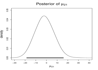
(b) Posterior of $\mu_{21}$.

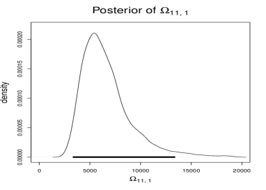
(c) Posterior of $\Omega_{11,1}$.

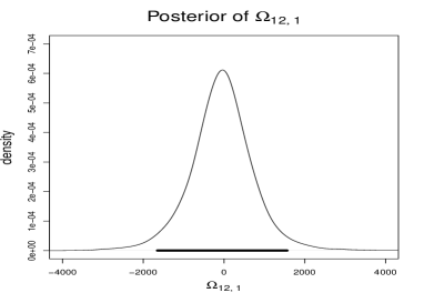
(d) Posterior of $\Omega_{12,1}$.

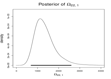
(e) Posterior of $\Omega_{22,1}$.

Figure 9.2: TTMCMC for the real data case: Posteriors of $\mu_{11}$, $\mu_{21}$, $\Omega_{11,1}$, $\Omega_{12,1}$ and $\Omega_{22,1}$.

(a) Realdata analysis: Histogram of the first co-ordinate of $\hat{\phi}_{i}$’s.

(b) Realdata analysis: Histogram of the second co-ordinate of $\hat{\phi}_{i}$’s.

Figure 9.3: Realdata analysis: Posterior predictive pointwise 95% credible intervals of the times series for the companies. The thick curves denote the actual data.

Figure 9.4: Realdata analysis: Posterior predictive pointwise 95% credible intervals of the times series for the companies. The thick curves denote the actual data.

10 Summary and discussion

In this work, we consider the random effect parameter having mixture of normal distributions. Inherent flexibility of the mixture framework offers far greater generality compared to normal distributions considered so far in this direction of research. Even in this setup we are able to prove strong consistency and asymptotic normality of the $MLE$ and in the corresponding Bayesian framework we establish posterior consistency and asymptotic normality of the posterior distribution, our results encompassing both $iid$ and non-$iid$ situations, for both the paradigms. It is important to note that no extra assumptions are needed besides the assumptions of Maitra and Bhattacharya (2016) and Maitra and Bhattacharya (2015) to conclude the corresponding results under the consideration of normal mixture. In other words, without any extra assumption we could achieve asymptotic results regarding the random effect parameters having a much larger class of distributions, which seems to hold importance from theoretical and practical perspectives. Importantly, we have also developed the Bayesian asymptotic theory when the number of mixture components is unknown and considered random.

Although Delattre et al. (2016) also considered the $SDE$ mixture model, they required an extra, strong assumption to prove even weak consistency of $MLE$ in the $iid$ setup, compared to our stronger, almost sure convergence result, without the assumption. Moreover, the weak consistency result in the $iid$ situation is the only asymptotic result they provided, while we delved into consistency and asymptotic normality of both $MLE$ and the Bayesian posterior distribution, in both $iid$ and non-$iid$ setups, even when the number mixture components is random.

In all our simulation studies and the real stock market data analysis we fitted the data assuming that the number of mixture components is unknown and implemented our Bayesian methodology with TTMCMC in those variable-dimensional models. Excellent performance of our methods in all the cases lead us to recommend the variable-dimensional Bayesian paradigm to be implemented with TTMCMC. In contrast, the classical $BIC$ based method of Delattre et al. (2016) often yielded poor performance when the number of mixtures is unknown.

In this work we have considered one dimensional $SDE$s. The generalization of our asymptotic theories to high dimensions will be considered in our future endeavors.

S-1 Proof that differentiation can be passed under the integral sign

Let us denote the marginal distribution of $\{X_{i}(t):t\in[0,T]\}$ by $Q_{\theta}^{i}$ on $(C_{T},\mathcal{C}_{T})$, where $C_{T}$ is the space of real continuous functions on $[0,T]$ and $\mathcal{C}_{T}$ is the corresponding $\sigma$-algebra. Recall that
$\theta=(\gamma,\beta)=(a_{1},\ldots,a_{M},\mu_{1},\ldots,\mu_{M},\omega_{1}^{2},\ldots,\omega_{M}^{2})$.

Let $\tau=(1,0,\ldots,0,\mu_{1}^{*},\ldots,\mu_{M}^{*},{\omega_{1}^{*}}^{2},\ldots,{\omega_{M}^{*}}^{2})$ and set

$$p_{1}(\theta) =\frac{\lambda_{1}(X_{1},\theta)}{\lambda_{1}(X_{1},\tau)}$$

$$=\frac{\sum_{k=1}^{M}\frac{a_{k}}{\left(1+\omega_{k}^{2}V_{1}\right)^{1/2}}\exp\left[-\frac{V_{1}}{2\left(1+\omega_{k}^{2}V_{1}\right)}\left(\mu_{k}-\frac{U_{1}}{V_{1}}\right)^{2}\right]\exp\left(\frac{U^{2}_{1}}{2V_{1}}\right)}{\frac{1}{\left(1+{\omega_{1}^{*}}^{2}V_{1}\right)^{1/2}}\exp\left[-\frac{V_{1}}{2\left(1+{\omega_{1}^{*}}^{2}V_{1}\right)}\left(\mu_{1}^{*}-\frac{U_{1}}{V_{1}}\right)^{2}\right]\exp\left(\frac{U^{2}_{1}}{2V_{1}}\right)}$$

$$=\sum_{k=1}^{M}\frac{a_{k}(1+{\omega_{1}^{*}}^{2}V_{1})^{\frac{1}{2}}}{(1+{\omega_{k}}^{2}V_{1})^{\frac{1}{2}}}\exp\left[-\frac{V_{1}}{2\left(1+\omega_{k}^{2}V_{1}\right)}\left(\mu_{k}-\frac{U_{1}}{V_{1}}\right)^{2}+\frac{V_{1}}{2\left(1+{\omega_{1}^{*}}^{2}V_{1}\right)}\left(\mu_{1}^{*}-\frac{U_{1}}{V_{1}}\right)^{2}\right]$$ (S-1.1)

so that $\int_{C_{T}}p_{1}(\theta)dQ_{\tau}^{1}=1$. The assurance of interchange of integration with respect to $Q_{\tau}^{1}$ and differentiation with respect to $\theta$ implies interchange of integration with respect to $Q_{\theta}^{1}$ and differentiation with respect to $\theta$. So, here we will justify interchange of integration with respect to $Q_{\tau}^{1}$ and differentiation with respect to $\theta$.

Note that

$$\frac{\partial p_{1}(\theta)}{\partial a_{k}}\leq(1+{\omega_{1}^{*}}^{2}V_{1})^{\frac{1}{2}}\exp\left[-\frac{V_{1}}{2\left(1+\omega_{k}^{2}V_{1}\right)}\left(\mu_{k}-\frac{U_{1}}{V_{1}}\right)^{2}+\frac{V_{1}}{2\left(1+{\omega_{1}^{*}}^{2}V_{1}\right)}\left(\mu_{1}^{*}-\frac{U_{1}}{V_{1}}\right)^{2}\right].$$ (S-1.2)

Let

$$\overline{\mu}^{2}=\max\{\mu^{2}_{k},{\mu_{1}^{*}}^{2}\};\quad\underline{\mu}^{2}=\min\{\mu^{2}_{k},{\mu_{1}^{*}}^{2}\};\quad\underline{\omega}=\min\{\omega_{k},\omega_{1}^{*}\}.$$

Now

$$\mu_{k}^{2}-2\mu_{k}\frac{U_{1}}{V_{1}}+\frac{U_{1}^{2}}{V_{1}^{2}}\geq\underline{\mu}^{2}-2\mu_{k}\frac{U_{1}}{V_{1}}+\frac{U_{1}^{2}}{V_{1}^{2}}$$

$$\implies-\left(\mu_{k}^{2}-2\mu_{k}\frac{U_{1}}{V_{1}}+\frac{U_{1}^{2}}{V_{1}^{2}}\right) \leq-\left(\underline{\mu}^{2}-2\mu_{k}\frac{U_{1}}{V_{1}}+\frac{U_{1}^{2}}{V_{1}^{2}}\right).$$ (S-1.3)

Also,

$${\mu_{1}^{*}}^{2}-2\mu_{1}^{*}\frac{U_{1}}{V_{1}}+\frac{U_{1}^{2}}{V_{1}^{2}}\leq\overline{\mu}^{2}-2\mu_{1}^{*}\frac{U_{1}}{V_{1}}+\frac{U_{1}^{2}}{V_{1}^{2}},$$ (S-1.4)

$$\frac{V_{1}}{2\left(1+\omega_{k}^{2}V_{1}\right)}\leq\frac{V_{1}}{2\left(1+\underline{\omega}^{2}V_{1}\right)}\quad\mbox{and}\quad\frac{V_{1}}{2\left(1+{\omega_{1}^{*}}^{2}V_{1}\right)}\leq\frac{V_{1}}{2\left(1+\underline{\omega}^{2}V_{1}\right)}.$$ (S-1.5)

Due to (S-1.3), (S-1.4) and (S-1.5) it follows that

$$\frac{\partial p_{1}(\theta)}{\partial a_{k}} \leq(1+{\omega_{1}^{*}}^{2}V_{1})^{\frac{1}{2}}\exp\left[-\frac{V_{1}}{2\left(1+\underline{\omega}^{2}V_{1}\right)}\left(\underline{\mu}^{2}-2\mu_{k}\frac{U_{1}}{V_{1}}+\frac{U_{1}^{2}}{V_{1}^{2}}\right)\right.$$

$$\quad\quad\quad\quad\quad\quad\quad\quad\quad\quad\left.+\frac{V_{1}}{2\left(1+\underline{\omega}^{2}V_{1}\right)}\left(\overline{\mu}^{2}-2\mu_{1}^{*}\frac{U_{1}}{V_{1}}+\frac{U_{1}^{2}}{V_{1}^{2}}\right)\right]$$

$$=(1+{\omega_{1}^{*}}^{2}V_{1})^{\frac{1}{2}}\exp\left[\frac{V_{1}}{2\left(1+\underline{\omega}^{2}V_{1}\right)}(\overline{\mu}^{2}-\underline{\mu}^{2})+\frac{U_{1}}{\left(1+\underline{\omega}^{2}V_{1}\right)}(\mu_{k}-\mu_{1}^{*})\right]$$

$$\leq(1+{\omega_{1}^{*}}^{2}V_{1})^{\frac{1}{2}}\exp\left[\frac{1}{2\underline{\omega}^{2}}(\overline{\mu}^{2}-\underline{\mu}^{2})+\frac{U_{1}}{\left(1+\underline{\omega}^{2}V_{1}\right)}(\mu_{k}-\mu_{1}^{*})\right]=K_{1}(U_{1},V_{1})~{}\mbox{(say)},$$

where the last inequality follows as $\frac{V_{1}}{2(1+\underline{\omega}^{2}V_{1})}<\frac{1}{2\underline{\omega}^{2}}$. Note that $K_{1}(U_{1},V_{1})$ has finite expectation, that is, integrable with respect to $Q_{\tau}^{1}$, thanks to existence of all order moments of $V_{1}$, Lemma 1 of Delattre et al. (2013), and the Cauchy-Schwartz inequality.

Further, with $\mu_{\max}=\max\left\{|\mu_{1}|,\ldots,|\mu_{M}|\right\}$, note that,

$$\left|\frac{\partial p_{1}}{\partial\mu_{k}}\right| \leq K_{1}(U_{1},V_{1})[V_{1}\mu_{\max}+|U_{1}|];$$ (S-1.6)

$$\left|\frac{\partial p_{1}}{\partial\omega_{k}^{2}}\right| \leq K_{1}(U_{1},V_{1})[V_{1}+(V_{1}\mu_{\max}+|U_{1}|)^{2}];$$ (S-1.7)

$$\left|\frac{\partial^{2}p_{1}}{\partial\mu_{k}^{2}}\right| \leq K_{1}(U_{1},V_{1})[V_{1}+(V_{1}\mu_{\max}+|U_{1}|)^{2}];$$ (S-1.8)

$$\left|\frac{\partial^{2}p_{1}}{\partial\omega_{k}^{2}\partial\omega_{k}^{2}}\right| \leq K_{1}(U_{1},V_{1})\left[V_{1}^{2}+3\left(V_{1}^{3/2}\mu_{\max}+V_{1}^{1/2}|U_{1}|\right)^{2}+\left(V_{1}\mu_{\max}+|U_{1}|\right)^{4}\right];$$ (S-1.9)

$$\left|\frac{\partial^{2}p_{1}}{\partial\mu_{k}\partial\omega_{k}^{2}}\right| \leq K_{1}(U_{1},V_{1})\left[2\left(V_{1}^{2}\mu_{\max}+V_{1}|U_{1}|\right)+(V_{1}\mu_{\max}+|U_{1}|)^{3}\right],$$ (S-1.10)

where each upper bound has finite expectation. This easily follows due to existence of all order moments of $V_{1}$ and $|U_{1}|$ (which follows from Lemma 1 of Delattre et al. (2013)), compactness of the parameter space, the fact that the expectation of $K_{1}(U_{1},V_{1})$ is finite, and the Cauchy-Schwartz inequality. Therefore, the interchange is justified.

S-2 Upper bounds of the third order partial derivatives of log-likelihood

Likelihood corresponding to the $i$-th individual is

$$\lambda_{i}(X_{i},\theta)=\sum_{k=1}^{M}a_{k}f(X_{i}|\beta_{k}),$$

where

$$f(X_{i}|\beta_{k})=\frac{1}{\left(1+\omega_{k}^{2}V_{i}\right)^{1/2}}\exp\left[-\frac{V_{i}}{2\left(1+\omega_{k}^{2}V_{i}\right)}\left(\mu_{k}-\frac{U_{i}}{V_{i}}\right)^{2}\right]\exp\left(\frac{U^{2}_{i}}{2V_{i}}\right).$$

Hence we obtain,

$$\left|\frac{f}{\lambda}\right| \leq 1;$$ (S-2.1)

$$\left|\frac{1}{\lambda}\frac{\partial f}{\partial\mu}\right| \leq\left[V\mu_{\max}+V|U|\right];$$ (S-2.2)

$$\left|\frac{1}{\lambda}\frac{\partial f}{\partial\omega^{2}}\right| \leq\left[V+\left(V\mu_{\max}+|U|\right)^{2}\right];$$ (S-2.3)

$$\left|\frac{1}{\lambda}\frac{\partial^{2}f}{\partial\mu^{2}}\right| \leq\left[V+\left(V\mu_{\max}+|U|\right)^{2}\right];$$ (S-2.4)

$$\left|\frac{1}{\lambda}\frac{\partial^{2}f}{\partial\omega^{2}\partial\omega^{2}}\right| \leq\left[V^{2}+3\left(V^{3/2}\mu_{\max}+V^{1/2}|U|\right)^{2}+\left(V\mu_{\max}+|U|\right)^{4}\right];$$ (S-2.5)

$$\left|\frac{1}{\lambda}\frac{\partial^{2}f}{\partial\mu\partial\omega^{2}}\right| \leq\left[2\left(V^{2}\mu_{\max}+V|U|\right)+\left(V\mu_{\max}+|U|\right)^{3}\right];$$ (S-2.6)

$$\left|\frac{1}{\lambda}\frac{\partial^{3}f}{\partial\mu^{3}}\right| \leq\left[3\left(V^{2}\mu_{\max}+V|U|\right)+\left(V\mu_{\max}+|U|\right)^{3}\right];$$ (S-2.7)

$$\left|\frac{1}{\lambda}\frac{\partial^{3}f}{\partial\mu^{2}\partial\omega^{2}}\right| \leq\left[2V^{2}+3\left(V^{3/2}\mu_{\max}+V^{1/2}|U|\right)^{2}+\left(V\mu_{\max}+|U|\right)^{4}\right];$$ (S-2.8)

$$\left|\frac{1}{\lambda}\frac{\partial^{3}f}{\partial\mu\partial\omega^{2}\partial\omega^{2}}\right| \leq\left[4\left(V^{3}\mu_{\max}+V^{2}|U|\right)+4\left(V^{4/3}\mu_{\max}+V^{1/3}|U|\right)^{3}+\left(V\mu_{\max}+|U|\right)^{5}\right];$$ (S-2.9)

$$\left|\frac{1}{\lambda}\frac{\partial^{3}f}{\partial\omega^{2}\partial\omega^{2}\partial\omega^{2}}\right| \leq\left[2V^{3}+11\left(V^{2}\mu_{\max}+V|U|\right)^{2}+5\left(V^{5/4}\mu_{\max}+V^{1/4}|U|\right)^{4}+\left(V\mu_{\max}+|U|\right)^{6}\right],$$ (S-2.10)

where each of the upper bounds has finite expectation. This can be seen from the existence of all order moments of $V$ and $|U|$ (which follows from Lemma 1 of Delattre et al. (2013)), along with the compactness of the parameter space, and using the Cauchy-Schwartz inequality.

S-3 Non-multiplicative random effects

So far we have considered systems of $SDE$s with multiplicative random effects given by (1.1). However, it is possible to consider models of the following form with non-multiplicative random effects (see, for example, Delattre et al. (2016)):

$$dX_{i}(t)=(\phi_{i}b(X_{i}(t))+a(X_{i}(t)))dt+\sigma(X_{i}(t))dW_{i}(t),\quad\mbox{with}\quad X_{i}(0)=x^{i},~{}i=1,\ldots,n,$$ (S-3.1)

Under the assumptions that $a(\cdot)$ and $b(\cdot)$ are Lipschitz continuous on $\mathbb{R}$, $\sigma(\cdot)$ is Holder continuous with exponent $\alpha\in\left[\frac{1}{2},1\right]$ on $\mathbb{R}$, and $\int_{0}^{T_{i}}\frac{b^{2}(X_{i}(s))+a^{2}(X_{i}(s))}{\sigma^{2}(X_{i}(s))}<\infty$ almost surely for $i\geq 1$, it follows that the form likelihood of the $i$-th individual remains the same as (2.1), with $V_{i}$ remaining the same as before and $U_{i}$ having the form $U_{i}=\int_{0}^{T_{i}}\frac{b(X_{i}(s))}{\sigma^{2}(X_{i}(s))}(dX_{i}(s)-a(X_{i}(s))ds)$. Note that this is the density with respect to the measure associated with (S-3.1) where $\phi_{i}=0$.

It is easy to perceive that all our asymptotic results with respect to (S-3.1) remain the same as before.

S-4 Multidimensional linear random effects

Here we consider $d$-dimensional random effect, that is, we consider $SDE$s of the following form:

$$dX_{i}(t)=\boldsymbol{\phi}^{T}_{i}\boldsymbol{b}(X_{i}(t))dt+\sigma(X_{i}(t))dW_{i}(t),\quad\mbox{with}\quad X_{i}(0)=x^{i},~{}i=1,\ldots,n.$$ (S-4.1)

where $\boldsymbol{\phi}_{i}=(\phi_{i}^{1},\phi_{i}^{2},\ldots,\phi_{i}^{d})^{T}$ is a $d$-dimensional random vector and $\boldsymbol{b}(x)=(b^{1}(x),b^{2}(x),\ldots,b^{d}(x))^{T}$ is a function from $\mathbb{R}$ to $\mathbb{R}^{d}$. Here $b(x,\varphi)=\sum_{i=1}^{d}\varphi^{i}b^{i}(x)$ satisfies (H1). We consider $\boldsymbol{\phi}_{i}$ having, say, $M$ mixture of normal distributions having expectation vectors $\boldsymbol{\mu}_{k}$ and covariance matrices $\boldsymbol{\Omega}_{k}$ for $k=1,\ldots,M$, with density

$$g(\varphi,\boldsymbol{\theta})d\nu(\varphi)\equiv\sum_{k=1}^{M}a_{k}N(\boldsymbol{\mu}_{k},\boldsymbol{\Omega}_{k})$$

such that $a_{k}\geq 0$ for $k=1,\ldots,M$ and $\sum_{k=1}^{M}a_{k}=1$. Here the parameter set is

$$\boldsymbol{\theta}=(a_{1},\boldsymbol{\mu}_{1},\boldsymbol{\Omega}_{1},\ldots,a_{M},\boldsymbol{\mu}_{M},\boldsymbol{\Omega}_{M})=(\gamma,\boldsymbol{\beta}),$$

where, $\gamma=(a_{1},\ldots,a_{M})$, and $\boldsymbol{\beta}=(\boldsymbol{\beta}_{1},\ldots,\boldsymbol{\beta}_{M})$, where, for $k=1,\ldots,M$, $\boldsymbol{\beta}_{k}=(\boldsymbol{\mu}_{k},\boldsymbol{\Omega}_{k})$.

The sufficient statistics for $i=1,\ldots,n$ are

$$\boldsymbol{U}_{i}=\int_{0}^{T_{i}}\frac{\boldsymbol{b}(X_{i}(s))}{\sigma^{2}(X_{i}(s))}dX_{i}(s)$$

and

$$\boldsymbol{V}_{i}=\int_{0}^{T_{i}}\frac{\boldsymbol{b}(X_{i}(s))\boldsymbol{b}^{T}(X_{i}(s))}{\sigma^{2}(X_{i}(s))}ds.$$

Note that $\boldsymbol{U}_{i}$ are $d$-dimensional random vectors and $\boldsymbol{V}_{i}$ are random matrices of order $d\times d$. As in Delattre et al. (2013) we need to assume that $\boldsymbol{V}_{i}$ is positive definite for each $i\geq 1$ and for all $\boldsymbol{\theta}$.

By Lemma 2 of Delattre et al. (2013) it follows, almost surely, for all $i\geq 1$, for $1\leq k\leq M$ and for all $\boldsymbol{\theta}$, that $\boldsymbol{V}_{i}+\boldsymbol{\Omega}_{k}^{-1},\mathbb{I}_{d}+\boldsymbol{V}_{i}\boldsymbol{\Omega}_{k},\mathbb{I}_{d}+\boldsymbol{\Omega}_{k}\boldsymbol{V}_{i}$ are invertible.

Setting $\boldsymbol{R}_{i}^{-1}=(\mathbb{I}_{d}+\boldsymbol{V}_{i}\boldsymbol{\Omega}_{k})^{-1}\boldsymbol{V}_{i}$ we have

$$\lambda_{i}(X_{i},\boldsymbol{\theta})=\sum_{i=1}^{M}a_{k}f(X_{i}|\boldsymbol{\beta}_{k}),$$ (S-4.2)

where

$$f(X_{i}|\boldsymbol{\beta}_{k})=\frac{1}{\sqrt{\det(\mathbb{I}_{d}+\boldsymbol{V}_{i}\boldsymbol{\Omega}_{k})}}\exp\left(-\frac{1}{2}(\boldsymbol{\mu}_{k}-\boldsymbol{V}_{i}^{-1}\boldsymbol{U}_{i})^{T}\boldsymbol{R}_{i}^{-1}(\boldsymbol{\mu}_{k}-\boldsymbol{V}_{i}^{-1}\boldsymbol{U}_{i})\right)\exp\left(\frac{1}{2}\boldsymbol{U}_{i}^{T}\boldsymbol{V}_{i}^{-1}\boldsymbol{U}_{i}\right)$$ (S-4.3)

The asymptotic investigation for both classical and Bayesian paradigms in this multidimensional case can be carried out in the same way as the one-dimensional problem, using Theorem 5 of Maitra and Bhattacharya (2016) with relevant modifications and Proposition 10 (i) of Delattre et al. (2013) which is valid here for each $(\boldsymbol{\mu}_{k},\boldsymbol{\Omega}_{k})$.

S-5 Simulation studies

For our convenience, we denote the $SDE$ models by the following: for $i\geq 1$ and $t\in[0,T]$,

$$SDE_{1}:~{}dX_{i}(t)=\phi_{i}X_{i}(t)dt+\sigma dW_{i}(t),~{}X_{i}(0)=x;$$ (S-5.1)

$$SDE_{2}:~{}dX_{i}(t)=(\phi_{i}-X_{i}(t))dt+\sigma dW_{i}(t),~{}X_{i}(0)=x;$$ (S-5.2)

$$SDE_{3}:~{}dX_{i}(t)=(\phi_{i}X_{i}(t)+2\sigma^{2})dt+2\sigma\sqrt{X_{i}(t)}dW_{i}(t),~{}X_{i}(0)=x.$$ (S-5.3)

As in Delattre et al. (2016), we choose $\sigma=0.1$, $x=1$, $T=1$. Note that although $SDE_{1}$ is of the form (1.1) with multiplicative random effect, $SDE_{2}$ abd $SDE_{3}$ are of the form (S-3.1). Unless otherwise stated, $n=100$. For sampling the discrete paths, we divide $[0,T]$ into $T/\delta$ intervals, each of length $\delta$. We set $\delta=0.0002$.

For the distribution of $\phi$, we choose the following 5 normal mixture distributions, as in Delattre et al. (2016):

$$\pi_{1}:~{}0.5N\left(-0.5,0.25^{2}\right)+0.5N\left(-1.8,0.25^{2}\right);$$ (S-5.4)

$$\pi_{2}:~{}0.7N\left(-0.5,0.5^{2}\right)+0.3N\left(-1.8,0.5^{2}\right);$$ (S-5.5)

$$\pi_{3}:~{}0.2N\left(-0.5,0.25^{2}\right)+0.3N\left(-3.5,0.25^{2}\right)+0.5N\left(-5.5,0.25^{2}\right);$$ (S-5.6)

$$\pi_{4}:~{}0.2N\left(-0.5,0.25^{2}\right)+0.3N\left(-1.8,0.25^{2}\right)+0.5N\left(-2.5,0.25^{2}\right);$$ (S-5.7)

$$\pi_{5}:~{}0.2N\left(-0.5,0.5^{2}\right)+0.3N\left(-1.8,0.5^{2}\right)+0.5N\left(-2.5,0.5^{2}\right).$$ (S-5.8)

S-5.1 Prior structure for our postulated mixture model

In all the simulation studies, we choose the uniform prior for $M$ on $\{1,2,\ldots,M_{\max}\}$, with $M_{\max}=30$. We reparameterize $\omega^{2}_{k}$ as $\omega^{2}_{k}=\exp(-\tau_{k})$, where $\tau_{k}\sim\log\left(\mathcal{G}\left(s/2,S/2\right)\right)$. Here, for positive $a$ and $b$, $\mathcal{G}(a,b)$ denotes the gamma distribution with mean $a/b$ and variance $a/b^{2}$. Given $\omega^{2}_{k}$, we assume that $[\mu_{k}|\omega^{2}_{k}]\sim N\left(\mu_{0},\psi\omega^{2}_{k}\right)$. For the prior on $a_{k}$’s, we write $a_{k}=\frac{\exp(w_{k})}{\sum_{j=1}^{M}\exp(w_{j})}$, where $w_{j}\stackrel{{\scriptstyle iid}}{{\sim}}N\left(\mu_{w},\sigma^{2}_{w}\right)$. All these choices are motivated by Das and Bhattacharya (2019). Further, we set the standard choices $s=S=2\times 0.1$ and $\mu_{w}=0$ in all our simulation experiments. We choose $\sigma^{2}_{w}$ to be $0.5$ and $0.35$ for the different simulation studies. These somewhat small variances reflect our belief that the $a_{k}$’s are approximately the same a priori. The values of $\psi$ and $\sigma^{2}_{w}$ are particularly chosen to ensure good mixing properties of TTMCMC and little uncertainty about the posterior of $M$. As it turned out, when $\pi_{1}$ and $\pi_{2}$ are the true models, $\psi=10$ and $\sigma^{2}_{w}=0.5$ achieved this purpose, while for $\pi_{3}$, $\pi_{4}$ and $\pi_{5}$, $\psi=100$ and $\sigma^{2}_{w}=0.35$ were the most appropriate in terms of ensuring good mixing and small uncertainty about $M$ a posteriori.

S-5.2 Implementation details

For TTMCMC, we implement Algorithm S-3.1 of the supplement of Das and Bhattacharya (2019), with additive transformation driven by the standard normal density on the positive part of the real line. We set equal probabilities for birth (emergence of a new mixture component), death (deletion of an existing mixture component) and no-change (no change to the number of mixture components) moves, and equal probabilities for the forward (addition of a scaled, positive standard normal variable to the current value of any given parameter co-ordinate) and backward (subtraction of a scaled, positive standard normal variable from the current value of any given parameter co-ordinate) transformations. We choose all the scales of the additive transformation to be $0.5$. As we shall demonstrate, these choices led to excellent mixing properties of our TTMCMC algorithm. For all the experiments, we discarded the first $15\times 10^{5}$ TTMCMC iterations as burn-in and stored one in 150 out of a further $15\times 10^{5}$ iterations to obtain $10000$ realizations from the variable-dimensional posteriors. Our codes, all written in $C$, are implemented on a 64-bit 4-core laptop with 7.6 GB memory, 2.3 GHz processor speed. When the true models are two-component mixtures, the entire TTMCMC implementation takes 2-3 minutes, while for the three component mixtures, our codes take 3-4 minutes. When $n=200$, as we consider in one of our simulation based illustrations, then it takes about 5 minutes for the two-component mixtures.

S-5.3 First simulation study: $SDE_{1}$ with $\pi_{1}$

Here we simulate data in accordance with $\pi_{1}$ and $SDE_{1}$ and fit our mixture model with a maximum of 30 components. The trace plots and the posterior density estimates of the parameters are provided in Figures S-5.1 and S-5.2, respectively.

The trace plots indicate excellent mixing of all the unknowns and the posterior plots in Figure S-5.2 show that all the true values, represented by the vertical lines fall well within the respective 95% credible regions, denoted by the thick horizontal line. The posterior probabilities of $M=2$ and $M=3$ turned out to be $0.8772$ and $0.1228$, respectively, and all other values of $M$ have zero posterior mass. Thus, the true value, $M_{0}=2$ receives significantly larger posterior probability compared to all the other values.

In other words, our Bayesian method puts up excellent performance in this experiment. Since the mixture components of $\pi_{1}$ are well-separated, this is to be expected.

The overall acceptance rate of our algorithm in this case is about $2\%$.

S-5.4 Second simulation study: $SDE_{1}$ with $\pi_{2}$

We now simulate the data in accordance with $\pi_{2}$ and $SDE_{1}$ and again fit our mixture model with a maximum of 30 components. Since the mixture components of $\pi_{2}$ are not as well-separated as in $\pi_{1}$, this setup is somewhat more challenging than the previous one.

However, the trace plots and the posterior density estimates of the parameters are provided in Figures S-5.3 and S-5.4, demonstrate excellent performance, despite the more challenging nature of the problem. The overall acceptance rate of our algorithm in this case is about $8\%$.

Here the posterior distribution of $M$ gave positive mass to $M=1,2,3$, with the respective probabilities being $0.2258$, $0.6391$ and $0.1351$. Although the posterior probability of $M=2$ is less than in the previous case of well-separated components, this is still very significantly large compared to the posterior probabilities of the other components, demonstrating that the Bayesian method has handled the challenge quite efficiently.

S-5.5 Third simulation study: $SDE_{2}$ with $\pi_{1}$

When the true model is given by $SDE_{2}$ and $\pi_{1}$, the trace plots and the posterior density estimates of the parameters are provided in Figures S-5.5 and S-5.6, respectively. The performance, as indicated by the plots, is again very satisfactory. Here $M=2$ and $M=3$ got the posterior probabilities $0.7549$ and $0.2451$, and all other values received the zero posterior probability. The overall acceptance rate in this case is about $2\%$.

S-5.6 Fourth simulation study: $SDE_{2}$ with $\pi_{2}$

In this case, the relevant diagrams provided in Figures S-5.7 and S-5.8, again indicate quite satisfactory performance. Here $M=2$ and $M=3$ received the posterior probabilities $0.8492$ and $0.1508$, respectively. The overall acceptance rate in this case is about $4\%$.

S-5.7 Fifth simulation study: $SDE_{2}$ with $\pi_{3}$

Figures S-5.9 and S-5.10, the relevant posterior plots associated with $SDE_{2}$ and $\pi_{3}$ indicate excellent mixing as before and satisfactory performance. The overall acceptance rate here is about $2\%$.

In this case, $M=3$ and $M=4$ received the posterior probabilities $0.8228$ and $0.1418$, respectively, while all the other values received the zero posterior probability.

S-5.8 Sixth simulation study: $SDE_{2}$ with $\pi_{4}$

In this case, the mixture components are not well-separated, and as demonstrated by Delattre et al. (2016), selection of $M$ by $BIC$ leads to unsatisfactory results. Our Bayesian approach, however, overcomes this challenge by acknowledging variable dimensionality and by employing TTMCMC. Figures S-5.11 and S-5.12, the relevant posterior plots associated with $SDE_{2}$ and $\pi_{4}$ indicate excellent mixing as before and satisfactory performance. The overall acceptance rate here is about $2.5\%$.

In this case, $M=2$, $M=3$ and $M=4$ received the posterior probabilities $0.0328$, $0.8138$ and $0.1534$, respectively, while all the other values received the zero posterior probability. In other words, our Bayesian approach successfully identifies the true number of components, unlike $BIC$.

S-5.9 Seventh simulation study: $SDE_{2}$ with $\pi_{5}$

In this example, the mixture components are severely ill-separated, and Table 4 of Delattre et al. (2016) shows that the $BIC$ approach in this case selects $1$ or $2$ mixture components, instead of the correct value $M_{0}=3$. However, our Bayesian approach based on TTMCMC again successfully captures the correct number of components. Indeed, $M=1,2,3,4$ received the posterior probabilities $0.0641$, $0.295$, $0.4668$ and $0.1505$, respectively. Figures S-5.13 and S-5.14 demonstrates quite adequate performance of our approach. The overall acceptance rate here is about $5.9\%$.

S-5.10 Eighth simulation study: $SDE_{3}$ with $\pi_{1}$

In this case as well, excellent mixing is vindicated by the trace plots shown in Figure S-5.15. Furthermore, as shown in Figure S-5.16, all the true values well-captured by our Bayesian approach. The posterior probabilities of $M=2$ and $M=3$ turned out to be $0.8629$ and $0.1371$, so that all other values of $M$ have zero posterior mass. The overall acceptance rate of our algorithm in this case is about $2.5\%$.

S-5.11 Ninth simulation study: $SDE_{3}$ with $\pi_{2}$

In this setup, as usual, excellent mixing is demonstrated by the trace plots shown in Figure S-5.17. However, Figure S-5.18 shows that the true values of $\mu_{2}$ and $\omega^{2}_{2}$ do not fall within the respective 95% credible intervals. Also, $M=1,2,3,4$ receive posterior mass $0.6840$, $0.2657$, $0.0444$ and $0.0059$, respectively, showing that the true number of components, $M_{0}=2$, does not receive the maximum posterior probability. An examination of the histogram of $\hat{\phi}_{i}=U_{i}/V_{i}$, shown in Figure 19(a), where the dark vertical lines represent the vales $-0.5$ and $-1.8$, reveals that it is indeed very difficult to identify $\mu_{2}=-1.8$, which is very ill-supported by the data. Consequently, the joint prior and posterior dependence between $\mu_{2}$ and $\omega^{2}_{2}$ seems to be responsible for pulling the significant posterior mass of $\omega^{2}_{2}$ away from the true value.

We repeated the experiment with $n=200$. The new histogram of $\hat{\phi}_{i}$, depicted in Figure 19(b), seems to be more informative about $\mu_{2}=-1.8$ than Figure 19(b). That the modified posterior probabilities of $M=1$ and $M=2$ are $0.0956$ and $0.9044$, respectively, with all other values of $M$ having zero posterior probability confirms this. Figure S-5.19 suggests excellent mixing as before and Figure S-5.20 shows that all the true values are now within the 95% credible intervals of the modified posterior.

The overall acceptance rate of our algorithm in this case is about $5.3\%$.

(a) Trace plot of $M$.

(b) Trace plot of $\mu_{1}$.

(c) Trace plot of $\mu_{2}$.

(d) Trace plot of $\omega^{2}_{1}$.

(e) Trace plot of $\omega^{2}_{2}$.

(f) Trace plot of $a_{1}$.

(g) Trace plot of $a_{2}$.

Figure S-5.1: TTMCMC for $SDE_{1}$ and $\pi_{1}$: Trace plots of $M$, $\mu_{1}$, $\mu_{2}$, $\omega^{2}_{1}$, $\omega^{2}_{2}$, $a_{1}$ and $a_{2}$.

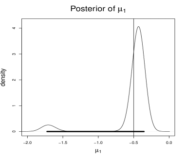
(a) Posterior of $\mu_{1}$.

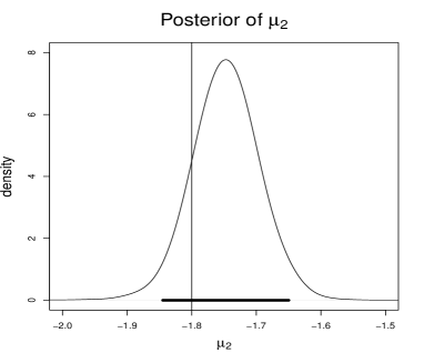
(b) Posterior of $\mu_{2}$.

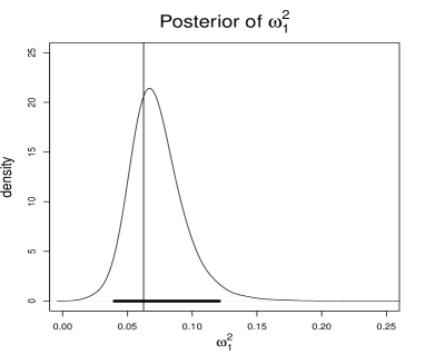
(c) Posterior of $\omega^{2}_{1}$.

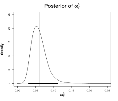
(d) Posterior of $\omega^{2}_{2}$.

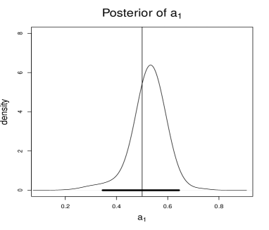
(e) Posterior of $a_{1}$.

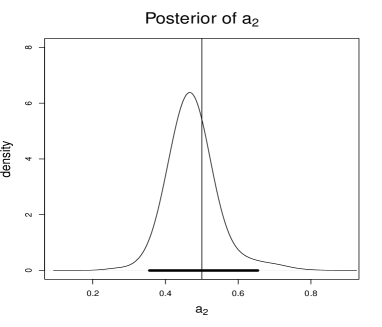
(f) Posterior of $a_{2}$.

Figure S-5.2: TTMCMC for $SDE_{1}$ and $\pi_{1}$: Posteriors of $M$, $\mu_{1}$, $\mu_{2}$, $\omega^{2}_{1}$, $\omega^{2}_{2}$, $a_{1}$ and $a_{2}$. The vertical lines stand for the true values, while the thick horizontal lines denote the 95% credible intervals.

(a) Trace plot of $M$.

(b) Trace plot of $\mu_{1}$.

(c) Trace plot of $\mu_{2}$.

(d) Trace plot of $\omega^{2}_{1}$.

(e) Trace plot of $\omega^{2}_{2}$.

(f) Trace plot of $a_{1}$.

(g) Trace plot of $a_{2}$.

Figure S-5.3: TTMCMC for $SDE_{1}$ and $\pi_{2}$: Trace plots of $M$, $\mu_{1}$, $\mu_{2}$, $\omega^{2}_{1}$, $\omega^{2}_{2}$, $a_{1}$ and $a_{2}$.

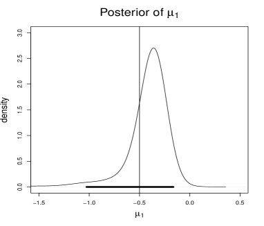
(a) Posterior of $\mu_{1}$.

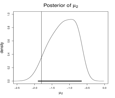
(b) Posterior of $\mu_{2}$.

(c) Posterior of $\omega^{2}_{1}$.

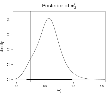
(d) Posterior of $\omega^{2}_{2}$.

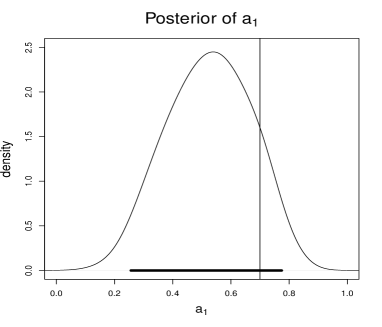
(e) Posterior of $a_{1}$.

(f) Posterior of $a_{2}$.

Figure S-5.4: TTMCMC for $SDE_{1}$ and $\pi_{2}$: Posteriors of $M$, $\mu_{1}$, $\mu_{2}$, $\omega^{2}_{1}$, $\omega^{2}_{2}$, $a_{1}$ and $a_{2}$. The vertical lines stand for the true values, while the thick horizontal lines denote the 95% credible intervals.

(a) Trace plot of $M$.

(b) Trace plot of $\mu_{1}$.

(c) Trace plot of $\mu_{2}$.

(d) Trace plot of $\omega^{2}_{1}$.

(e) Trace plot of $\omega^{2}_{2}$.

(f) Trace plot of $a_{1}$.

(g) Trace plot of $a_{2}$.

Figure S-5.5: TTMCMC for $SDE_{2}$ and $\pi_{1}$: Trace plots of $M$, $\mu_{1}$, $\mu_{2}$, $\omega^{2}_{1}$, $\omega^{2}_{2}$, $a_{1}$ and $a_{2}$.

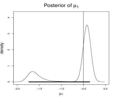
(a) Posterior of $\mu_{1}$.

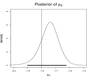
(b) Posterior of $\mu_{2}$.

(c) Posterior of $\omega^{2}_{1}$.

(d) Posterior of $\omega^{2}_{2}$.

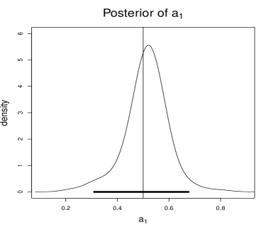
(e) Posterior of $a_{1}$.

(f) Posterior of $a_{2}$.

Figure S-5.6: TTMCMC for $SDE_{2}$ and $\pi_{1}$: Posteriors of $M$, $\mu_{1}$, $\mu_{2}$, $\omega^{2}_{1}$, $\omega^{2}_{2}$, $a_{1}$ and $a_{2}$. The vertical lines stand for the true values, while the thick horizontal lines denote the 95% credible intervals.

(a) Trace plot of $M$.

(b) Trace plot of $\mu_{1}$.

(c) Trace plot of $\mu_{2}$.

(d) Trace plot of $\omega^{2}_{1}$.

(e) Trace plot of $\omega^{2}_{2}$.

(f) Trace plot of $a_{1}$.

(g) Trace plot of $a_{2}$.

Figure S-5.7: TTMCMC for $SDE_{2}$ and $\pi_{2}$: Trace plots of $M$, $\mu_{1}$, $\mu_{2}$, $\omega^{2}_{1}$, $\omega^{2}_{2}$, $a_{1}$ and $a_{2}$.

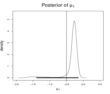
(a) Posterior of $\mu_{1}$.

(b) Posterior of $\mu_{2}$.

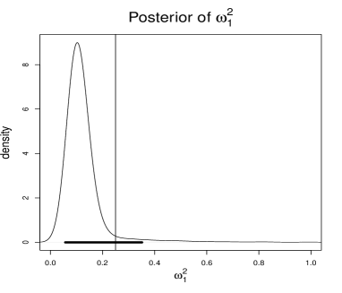
(c) Posterior of $\omega^{2}_{1}$.

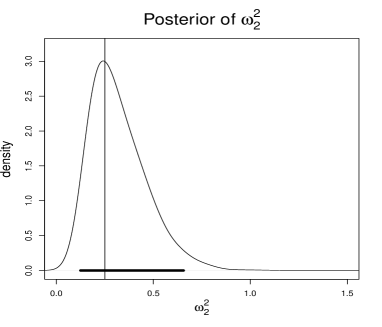
(d) Posterior of $\omega^{2}_{2}$.

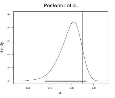
(e) Posterior of $a_{1}$.

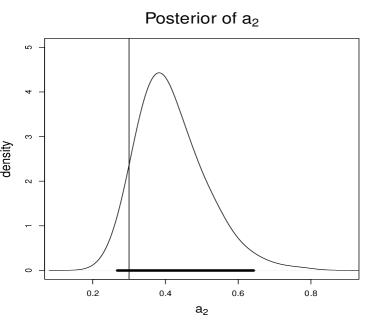
(f) Posterior of $a_{2}$.

Figure S-5.8: TTMCMC for $SDE_{2}$ and $\pi_{2}$: Posteriors of $M$, $\mu_{1}$, $\mu_{2}$, $\omega^{2}_{1}$, $\omega^{2}_{2}$, $a_{1}$ and $a_{2}$. The vertical lines stand for the true values, while the thick horizontal lines denote the 95% credible intervals.

(a) Trace plot of $M$.

(b) Trace plot of $\mu_{1}$.

(c) Trace plot of $\mu_{2}$.

(d) Trace plot of $\mu_{3}$.

(e) Trace plot of $\omega^{2}_{1}$.

(f) Trace plot of $\omega^{2}_{2}$.

(g) Trace plot of $\omega^{2}_{3}$.

(h) Trace plot of $a_{1}$.

(i) Trace plot of $a_{2}$.

(j) Trace plot of $a_{3}$.

Figure S-5.9: TTMCMC for $SDE_{2}$ and $\pi_{3}$: Trace plots of $M$, $\mu_{1}$, $\mu_{2}$, $\nu_{3}$, $\omega^{2}_{1}$, $\omega^{2}_{2}$, $\omega^{2}_{3}$, $a_{1}$ $a_{2}$ and $a_{3}$.

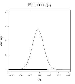
(a) Posterior of $\mu_{1}$.

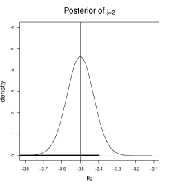
(b) Posterior of $\mu_{2}$.

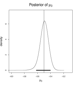
(c) Posterior of $\mu_{3}$.

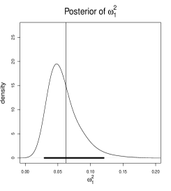
(d) Posterior of $\omega^{2}_{1}$.

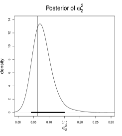
(e) Posterior of $\omega^{2}_{2}$.

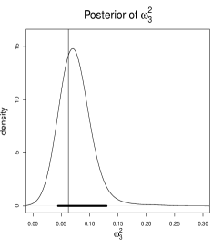
(f) Posterior of $\omega^{2}_{3}$.

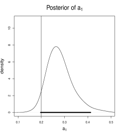
(g) Posterior of $a_{1}$.

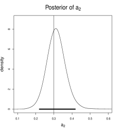
(h) Posterior of $a_{2}$.

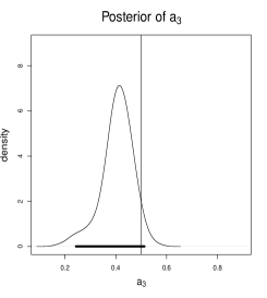
(i) Posterior of $a_{3}$.

Figure S-5.10: TTMCMC for $SDE_{2}$ and $\pi_{3}$: Posteriors of $M$, $\mu_{1}$, $\mu_{2}$, $\mu_{3}$, $\omega^{2}_{1}$, $\omega^{2}_{2}$, $\omega^{2}_{3}$, $a_{1}$ $a_{2}$ and $a_{3}$. The vertical lines stand for the true values, while the thick horizontal lines denote the 95% credible intervals.

(a) Trace plot of $M$.

(b) Trace plot of $\mu_{1}$.

(c) Trace plot of $\mu_{2}$.

(d) Trace plot of $\mu_{3}$.

(e) Trace plot of $\omega^{2}_{1}$.

(f) Trace plot of $\omega^{2}_{2}$.

(g) Trace plot of $\omega^{2}_{3}$.

(h) Trace plot of $a_{1}$.

(i) Trace plot of $a_{2}$.

(j) Trace plot of $a_{3}$.

Figure S-5.11: TTMCMC for $SDE_{2}$ and $\pi_{4}$: Trace plots of $M$, $\mu_{1}$, $\mu_{2}$, $\nu_{3}$, $\omega^{2}_{1}$, $\omega^{2}_{2}$, $\omega^{2}_{3}$, $a_{1}$ $a_{2}$ and $a_{3}$.

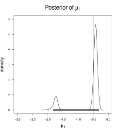
(a) Posterior of $\mu_{1}$.

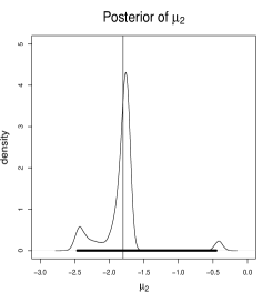
(b) Posterior of $\mu_{2}$.

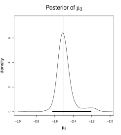
(c) Posterior of $\mu_{3}$.

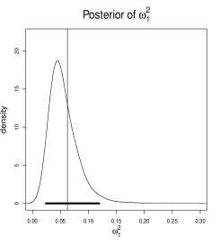
(d) Posterior of $\omega^{2}_{1}$.

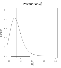
(e) Posterior of $\omega^{2}_{2}$.

(f) Posterior of $\omega^{2}_{3}$.

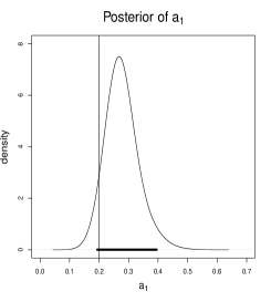
(g) Posterior of $a_{1}$.

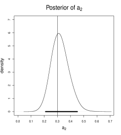
(h) Posterior of $a_{2}$.

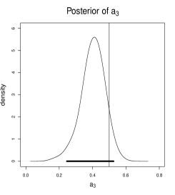
(i) Posterior of $a_{3}$.

Figure S-5.12: TTMCMC for $SDE_{2}$ and $\pi_{4}$: Posteriors of $M$, $\mu_{1}$, $\mu_{2}$, $\mu_{3}$, $\omega^{2}_{1}$, $\omega^{2}_{2}$, $\omega^{2}_{3}$, $a_{1}$ $a_{2}$ and $a_{3}$. The vertical lines stand for the true values, while the thick horizontal lines denote the 95% credible intervals.

(a) Trace plot of $M$.

(b) Trace plot of $\mu_{1}$.

(c) Trace plot of $\mu_{2}$.

(d) Trace plot of $\mu_{3}$.

(e) Trace plot of $\omega^{2}_{1}$.

(f) Trace plot of $\omega^{2}_{2}$.

(g) Trace plot of $\omega^{2}_{3}$.

(h) Trace plot of $a_{1}$.

(i) Trace plot of $a_{2}$.

(j) Trace plot of $a_{3}$.

Figure S-5.13: TTMCMC for $SDE_{2}$ and $\pi_{5}$: Trace plots of $M$, $\mu_{1}$, $\mu_{2}$, $\nu_{3}$, $\omega^{2}_{1}$, $\omega^{2}_{2}$, $\omega^{2}_{3}$, $a_{1}$ $a_{2}$ and $a_{3}$.

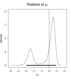
(a) Posterior of $\mu_{1}$.

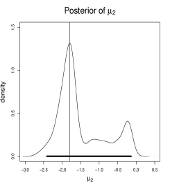
(b) Posterior of $\mu_{2}$.

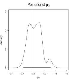
(c) Posterior of $\mu_{3}$.

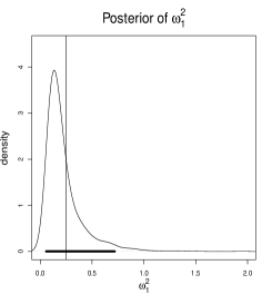
(d) Posterior of $\omega^{2}_{1}$.

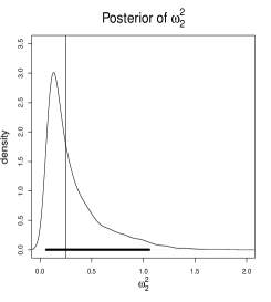
(e) Posterior of $\omega^{2}_{2}$.

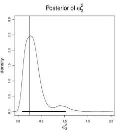
(f) Posterior of $\omega^{2}_{3}$.

(g) Posterior of $a_{1}$.

(h) Posterior of $a_{2}$.

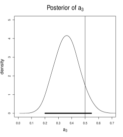
(i) Posterior of $a_{3}$.

Figure S-5.14: TTMCMC for $SDE_{2}$ and $\pi_{5}$: Posteriors of $M$, $\mu_{1}$, $\mu_{2}$, $\mu_{3}$, $\omega^{2}_{1}$, $\omega^{2}_{2}$, $\omega^{2}_{3}$, $a_{1}$ $a_{2}$ and $a_{3}$. The vertical lines stand for the true values, while the thick horizontal lines denote the 95% credible intervals.

(a) Trace plot of $M$.

(b) Trace plot of $\mu_{1}$.

(c) Trace plot of $\mu_{2}$.

(d) Trace plot of $\omega^{2}_{1}$.

(e) Trace plot of $\omega^{2}_{2}$.

(f) Trace plot of $a_{1}$.

(g) Trace plot of $a_{2}$.

Figure S-5.15: TTMCMC for $SDE_{3}$ and $\pi_{1}$: Trace plots of $M$, $\mu_{1}$, $\mu_{2}$, $\omega^{2}_{1}$, $\omega^{2}_{2}$, $a_{1}$ and $a_{2}$.

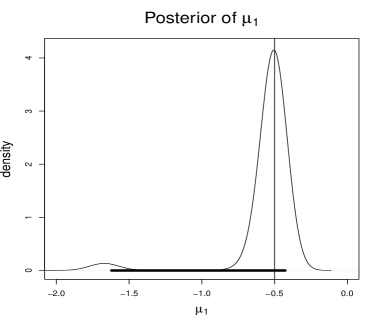
(a) Posterior of $\mu_{1}$.

(b) Posterior of $\mu_{2}$.

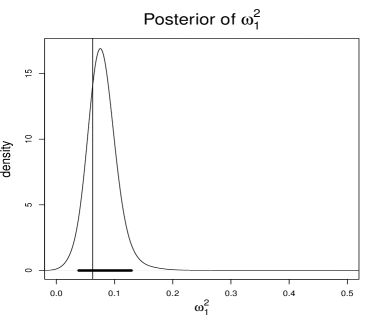
(c) Posterior of $\omega^{2}_{1}$.

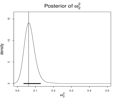
(d) Posterior of $\omega^{2}_{2}$.

(e) Posterior of $a_{1}$.

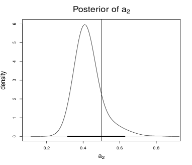
(f) Posterior of $a_{2}$.

Figure S-5.16: TTMCMC for $SDE_{3}$ and $\pi_{1}$: Posteriors of $M$, $\mu_{1}$, $\mu_{2}$, $\omega^{2}_{1}$, $\omega^{2}_{2}$, $a_{1}$ and $a_{2}$. The vertical lines stand for the true values, while the thick horizontal lines denote the 95% credible intervals.

(a) Trace plot of $M$.

(b) Trace plot of $\mu_{1}$.

(c) Trace plot of $\mu_{2}$.

(d) Trace plot of $\omega^{2}_{1}$.

(e) Trace plot of $\omega^{2}_{2}$.

(f) Trace plot of $a_{1}$.

(g) Trace plot of $a_{2}$.

Figure S-5.17: TTMCMC for $SDE_{3}$ and $\pi_{2}$ with $n=100$: Trace plots of $M$, $\mu_{1}$, $\mu_{2}$, $\omega^{2}_{1}$, $\omega^{2}_{2}$, $a_{1}$ and $a_{2}$.

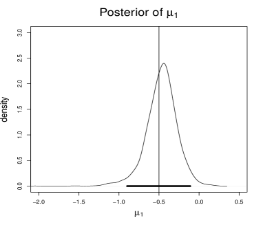
(a) Posterior of $\mu_{1}$.

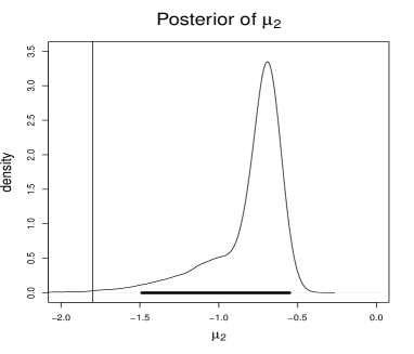
(b) Posterior of $\mu_{2}$.

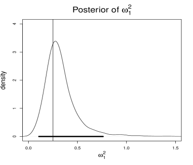
(c) Posterior of $\omega^{2}_{1}$.

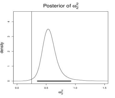
(d) Posterior of $\omega^{2}_{2}$.

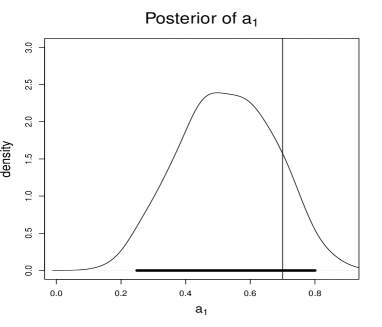
(e) Posterior of $a_{1}$.

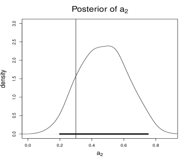
(f) Posterior of $a_{2}$.

Figure S-5.18: TTMCMC for $SDE_{3}$ and $\pi_{2}$ with $n=100$: Posteriors of $M$, $\mu_{1}$, $\mu_{2}$, $\omega^{2}_{1}$, $\omega^{2}_{2}$, $a_{1}$ and $a_{2}$. The vertical lines stand for the true values, while the thick horizontal lines denote the 95% credible intervals.

(a) Histogram of $\hat{\phi}_{i}$’s with $n=100$. The vertical lines denote the true values.

(b) Histogram of $\hat{\phi}_{i}$’s, with $n=200$. The vertical lines denote the true values.

(c) Trace plot of $M$.

(d) Trace plot of $\mu_{1}$.

(e) Trace plot of $\mu_{2}$.

(f) Trace plot of $\omega^{2}_{1}$.

(g) Trace plot of $\omega^{2}_{2}$.

(h) Trace plot of $a_{1}$.

(i) Trace plot of $a_{2}$.

Figure S-5.19: TTMCMC for $SDE_{3}$ and $\pi_{2}$ with $n=200$: Trace plots of $M$, $\mu_{1}$, $\mu_{2}$, $\omega^{2}_{1}$, $\omega^{2}_{2}$, $a_{1}$ and $a_{2}$.

(a) Posterior of $\mu_{1}$.

(b) Posterior of $\mu_{2}$.

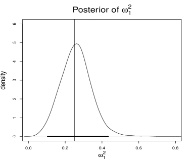
(c) Posterior of $\omega^{2}_{1}$.

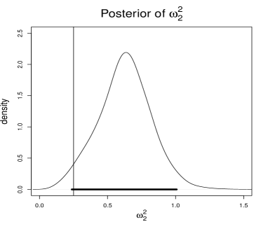
(d) Posterior of $\omega^{2}_{2}$.

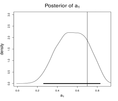
(e) Posterior of $a_{1}$.

(f) Posterior of $a_{2}$.

Figure S-5.20: TTMCMC for $SDE_{3}$ and $\pi_{2}$ with $n=200$: Posteriors of $M$, $\mu_{1}$, $\mu_{2}$, $\omega^{2}_{1}$, $\omega^{2}_{2}$, $a_{1}$ and $a_{2}$. The vertical lines stand for the true values, while the thick horizontal lines denote the 95% credible intervals.

References

- Atienza et al. (2005) Atienza, N., J., J. G.-H., Munoz-Pichardo, J., and Villa, R. (2005). Some Integrability Results on Exponential Families. Technical report. Available at “http://www.personal.us.es/natienza/inves/docu/technical1.pdf”.
- Banfield and Raftery (1993) Banfield, J. and Raftery, A. (1993). Model Based Gaussian and non-Gaussian Clustering. Biometrics, 49, 803–821.
- Bishop (1995) Bishop, C. M. (1995). Neural Networks for Pattern Recognition. Oxford University Press.
- Brooks (2001) Brooks, S. (2001). On Bayesian Analyses and Finite Mixtures for Proportions. Statistics and Computing, 11, 179–190.
- Chan et al. (1992) Chan, K. C., Karolyi, G. A., Longstaff, F. A., and Sanders, A. B. (1992). An Empirical Comparison of Alternative Models of the Short-Term Interest Rate. The Journal of Finance, 47, 1209–1227.
- Choi and Schervish (2007) Choi, T. and Schervish, M. J. (2007). On Posterior Consistency in Nonparametric Regression Problems. Journal of Multivariate Analysis, 98, 1969–1987.
- Das and Bhattacharya (2019) Das, M. and Bhattacharya, S. (2019). Transdimensional Transformation based Markov Chain Monte Carlo. Brazilian Journal of Probability and Statistics, 33, 87–138.
- Delattre et al. (2013) Delattre, M., Genon-Catalot, V., and Samson, A. (2013). Maximum Likelihood Estimation for Stochastic Differential Equations with Random Effects. Scandinavian Journal of Statistics, 40, 322–343.
- Delattre et al. (2016) Delattre, M., Genon-Catalot, V., and Samson, A. (2016). Mixtures of Stochastic Differential Equations With Random Effects: Application to Data Clustering. Journal of Statistical Planning and Inference, 173, 109–124.
- Dempster et al. (1977) Dempster, A., Laird, N., and Rubin, D. (1977). Maximum Likelihood from Incomplete Data via the EM Algorithm (with discussion). Journal of the Royal Statistical Society. Series B, 39, 1–38.
- Green and Richardson (2002) Green, P. and Richardson, S. (2002). Hidden Markov Models and Disease Mapping. Journal of the American Statistical Association, 97, 1055–1070.
- Green (1995) Green, P. J. (1995). Reversible jump Markov chain Monte Carlo computation and Bayesian model determination. Biometrika, 82, 711–732.
- Hoadley (1971) Hoadley, B. (1971). Asymptotic Properties of Maximum Lilelihood Estimators for the Independent not Identically Distributed Case. The Annals of Mathematical Statistics, 42, 1977–1991.
- Kass and Raftery (1995) Kass, R. E. and Raftery, R. E. (1995). Bayes factors. Journal of the American Statistical Association, 90(430), 773–795.
- Keribin (2000) Keribin, C. (2000). Consistent Estimation of the Order of Mixture Models Mixture Models. Sankhya, 62, 49–66.
- Leroux (1992) Leroux, B. (1992). Maximum Penalized Likelihood Estimation for Independent and Markov-Dependent Mixture Models. Biometrics, 48, 545–558.
- Lindsay (1995) Lindsay, B. (1995). Mixture Models: Theory Geometry and Applications. IMS, Hayward, CA.
- Louzada-Neto et al. (2002) Louzada-Neto, F., Mazucheli, J., and Achcar, J. (2002). Mixture Hazard Models for Lifetime Data. Biometrical Journal, 44, 3–14.