Better lower bounds for missing species: improved non-parametric moment-based estimation for large experiments

Abstract

Estimation of the number of species or unobserved classes from a random sample of the underlying population is a ubiquitous problem in statistics. In classical settings, the size of the sample is usually small. New technologies such as high-throughput DNA sequencing have allowed for the sampling of extremely large and heterogeneous populations at scales not previously attainable or even considered. New algorithms are required that take advantage of the size of the data to account for heterogeneity, but are also sufficiently fast and scale well with large data. We present a non-parametric moment-based estimator that is both computationally efficient and is sufficiently flexible to account for heterogeneity in the abundances of underlying population. This estimator is based on an extension of a popular moment-based lower bound (Chao, 1984), originally developed by Harris (1959) but unattainable due to the lack of economical algorithms to solve the system of nonlinear equation required for estimation. We apply results from the classical moment problem to show that solutions can be obtained efficiently, allowing for estimators that are simultaneously conservative and use more information. This is critical for modern genomic applications, where there may be many large experiments that require the application of species estimation. We present applications of our estimator to estimating T-Cell receptor repertoire and dropout in single cell RNA-seq experiments.

1 Introduction

Consider the problem of the estimating the number of distinct classes in an unknown population through sampling. Researchers sample instances from a finite and closed population and use the pattern of repeated sampling to estimate the number of unsampled classes. This problem is ubiquitous, with applications in immunology (Qi et al., 2014), microbiology (Bunge et al., 2014), epidemiology (Böhning and Schön, 2005), linguistics (Efron and Thisted, 1976), genetics (Gravel, 2014), database management (Haas et al., 1995), among others. See Deng et al. (2019) for a review of applications arising from high-throughput DNA sequencing data.

The original, and still primary, use of this problem was in ecology (Fisher et al., 1943) and most of the language and terminology arise from this application. The distinct classes are known as species and the instances are known as individuals. In such experiments, captures may be are costly and difficult. The total number of samples is typically in the hundreds or thousands. For example in Fisher et al. (1943), 620 species of butterfly were captured from the Malay peninsula, and more recently Gopalakrishnan et al. (2018) captured 1,436 microbial species (as determined by operational taxonomic units) in human patients. The small sample size results in very few degrees of freedom for identifying and estimating heterogeneity in the population. Estimators tend to focus on mild heterogeneity, such as simple contamination that results in small deviations from uniform sampling (Böhning et al., 2013; Chiu et al., 2014). When the number of samples is small, then approximating the non-uniformity with simple distributions may be appropriate because of the fact that it’s difficult to model complex heterogeneity when the data is small. On the other hand, when the sample size is large, say in the millions or billions, then researchers have a better opportunity to account for this heterogeneity and better estimate the number of unobserved species.

In our applications of interest, which arise from high-throughput sequencing experiments that sample millions or billions of DNA molecules, uniformity of the population is a hopeless thought. There are a myriad of inherent biases from the sequencing technology that vary between samples (Sims et al., 2014), in addition to the fact that the most interesting biology to study are typically the ones that inherently contain a large number of extremely rare classes (Bunge et al., 2014; Qi et al., 2014). Consider the following example: T-cell receptor (TCR) $\beta$ CDR3 clonotypes were interrogated in 39 individuals of various ages using high-thoughput sequencing (Britanova et al., 2014). In one sample, presented in Table 1, a total of 992,830 TCR $\beta$ CDR3 sequences were sampled with 705,621 distinct clones (or classes). The other samples in the study are also of similar size. The need for fast and accurate estimation is required for further analysis, such as age and environmental related patterns in TCR diversity.

$j$	1	2	3	4	5	6	7	…	3400	7288	7733
$n_{j}$	603,776	73,628	14,113	3,691	2,446	1,612	1, 148	…	1	1	1

Table 1: Example T-cell $\beta$ receptor count frequencies in a healthy 11 year old female.

There are several estimators currently available available for researchers. The non-parametric maximum likelihood estimator (NPMLE) of Norris and Pollock (1998) fits the discrete MLE under a Poisson model. Due to the inherent instability of this procedure that may result in a component with arbitrarily small abundance, Wang and Lindsay (2005) developed a penalized version of the non-parametric MLE, as the penalization helps to prevent the boundary problem in the NPMLE. Willis and Bunge (2015) presented a method based on non-linear regression of successive frequency ratios. Efron and Thisted (1976) derived a linear programming based lower bound. Burnham and Overton (1978) developed a jackknife-based estimator. But the most widely used estimator is a moment-based non-parameteric lower bound from Chao (1984). This estimator is easy to compute and is fairly robust to small deviations from homogeneity (Chao, 1977). Unfortunately, it only uses a small amount of information of the sample, just the number of species observed exactly once and twice, and will severely underestimate the population size when the population is highly heterogeneous.

Here we present a moment-based non-parametric method to extend Chao’s lower bound by taking into account more information available in the experiment. We first note that in a Poisson or multinomial mixture model, Chao’s lower bound is a special case of a general framework proposed by Harris (1959). In this framework the problem of estimating the number of unobserved classes is reformulated to the problem of estimating an integral of an unknown measure and the information in the sampled counts is reformulated into information on the unknown measure’s moments.

The problem of estimating an integral over an unknown measure with specified moments is well known in the numerical analysis literature and has a solution given by Gaussian quadrature. Gaussian quadrature can produce upper and lower bounds to the integral of interest using discrete approximations that are calculated via moment matching and the technique is intimately related to the classical moment problem (Golub and Meurant, 2010). This connection between the two problems allows us to extend the theory of the classical moment problem and advanced algorithms of Gaussian quadrature specifically for the problem of estimating the number of unobserved classes in a population. We will show that this allows us to obtain estimates that improve upon the Chao estimator in diverse and heterogeneous populations.

We present two applications of our estimator to problems in modern genomics: estimation of TCR repertoire, where species abundance is naturally highly heterogeneous, and estimation of dropout for single cell RNA-seq (scRNA-seq) experiments. In the former case we show that patterns in TCR repertoire may be missed using the observed repertoire that appear in the species-corrected repertoire. In the latter case, dropout is a consequence of the single cell sampling technology and can bias downstream analysis. We show in simulations that taking into account the species-corrected dropout in the differential expression analysis can improve identification of truly differentially differentially expressed genes.

The remainder of the paper is organized as follows. Section 2 introduces the underlying model and problem. Section 3 introduces our moment-based solution to estimating the number of unobserved classes and discusses Gaussian quadrature algorithms for computing the estimator. Section 4 shows results and comparisons to other estimators in the simple case where the abundance distribution is a discrete mixture distribution. Section 5 discusses a bagging strategy to alleviate an ill-conditioning issue with our estimator. Section 6 shows two applications of estimating the number of classes in high-throughput biology. We conclude with some remarks and discussions in section 7. Throughout the paper, for the sake of brevity we state the necessary theory without proofs, referring the reader instead to the requisite references.

2 Model

Consider a population of $S<\infty$ classes or species. In practice $S$ is an integer, but in the theory below we will let it be any number between zero and infinity. Let $y_{i}$ be the number of sampled individuals from class $i$, for $i=1,\ldots,S$, and let $N=\sum_{i=1}^{S}y_{i}$ be the total number of sampled individuals, sometimes called the sampling effort. We assume that $\bm{y}=\{y_{i};i=1,\ldots,S\}$ arise as independent Poisson random variables with rates $\bm{\lambda}=\{\lambda_{i};i=1,\ldots,S\}$. In the applications we consider, where the samples originate from high-throughput sequencing technologies, this assumption is appropriate since the total number of individuals sampled is inherently random.

If all species are equally abundant, then $\lambda_{1}=\lambda_{2}=\ldots=\lambda_{S}$. This situation is well-studied in the literature (Bunge and Fitzpatrick, 1993), but the equal abundance assumption is not likely to hold in practice. We assume that the Poisson rates are independently and identically distributed according to some latent distribution $\mu(\lambda)$, so that the sampled class counts will follow a Poisson mixture model. The latent mixing distribution encompasses all factors that may affect the abundance of classes, including both fundamental factors, such as the underlying biology (Desponds et al., 2016), and technical factors, such as PCR amplification bias (Benjamini and Speed, 2012).

Define $f_{\mu}(j)=\int_{0}^{\infty}e^{-\lambda}\lambda^{j}/j!\,d\mu(\lambda)$ to be the probability that a randomly chosen class is sampled exactly $j$ times. Let the count frequency $n_{j}$ be the number of classes with exactly $j$ individuals sampled, $n_{j}=\sum_{i=1}^{S}\mathbbm{1}\big{(}y_{i}=j\big{)}$ with expectation equal to

$$\mathrm{E}\big{(}n_{j}\big{)}=Sf_{\mu}(j)=S\int_{0}^{\infty}e^{-\lambda}\lambda^{j}/j!\,d\mu(\lambda).$$

Note that $n_{0}$ is the number of unobserved classes and since $S=n_{0}+\sum_{j=1}^{N}n_{j}$, estimating $n_{0}$ is equivalent to estimating $S$.

2.1 Harris’ change of measure

Following an idea presented by Harris (1959) and Chao (1984), we define the measure $\nu$ as a transformation of the abundance distribution $\mu$ such that

$$d\nu(\lambda)=S\,\lambda e^{-\lambda}d\mu(\lambda).$$

Note that $\nu$ is not a probability measure since it is unnormalized with $\int_{0}^{\infty}d\nu(\lambda)=\mathrm{E}n_{1}$. By definition this is a bijection with $d\mu(\lambda)=S^{-1}\,\lambda^{-1}e^{\lambda}d\nu(\lambda)$ and the support of $\mu$ and $\nu$ are identical.

The main benefit of defining and working with the transformed measure $\nu$ is that the moments of $\nu$ can be expressed as simple functions of the expected counts frequencies. Specifically the expected moments of $\nu$ can be derived as

$$\nu_{m}=\int_{0}^{\infty}\lambda^{m}d\nu(\lambda)=S\int_{0}^{\infty}\lambda^{m+1}e^{-\lambda}d\mu(\lambda)=(m+1)!\,\mathrm{E}\big{(}n_{m+1}\big{)},$$ (1)

with $\hat{\nu}_{m}=(m+1)!n_{m+1}$ denoting the estimated moments by plugging in the observed count frequencies for the expected count frequencies. Furthermore, we can express $\mathrm{E}(n_{0})$ in terms of the modified measure $\nu$ as

$$\mathrm{E}\big{(}n_{0}\big{)} =S\int_{0}^{\infty}e^{-\lambda}d\mu(\lambda)=\int_{0}^{\infty}\frac{1}{\lambda}\,S\lambda e^{-\lambda}d\mu(\lambda)$$

$$=\int_{0}^{\infty}\lambda^{-1}d\nu(\lambda).$$ (2)

This expression is free of $S$, since it has been absorbed into the unnormalized measure $\nu$. The estimation of $\mathrm{E}(n_{0})$ is now equivalent to estimation of the integral $\int_{0}^{\infty}\lambda^{-1}d\nu(\lambda)$.

The information we have on $\nu$ from the data is through the moments, which we can estimate by using the observed count frequencies. We now state the problem of estimating the number of missing species $n_{0}$ in the form of a moment-constrained problem as follows:

Estimate $$\int_{0}^{\infty}\lambda^{-1}d\nu(\lambda)$$ (3)

such that $$\hat{\nu}_{m}=(m+1)!n_{m+1}~{}\text{for}~{}m=0,1,\ldots,M.$$

We will refer to $M$ as the order of the estimate.

3 Moment spaces

Consider the space of all measures on the positive real line that satisfy the expected moment constraints in equation (3),

$$\mathcal{V}_{M}=\{\xi:\xi\text{ is a measure on the positive reals and }\xi_{m}=\nu_{m}~{}\text{for}~{}m=0,1,\ldots,M\},$$

called a $M$-truncated moment space. $\mathcal{V}_{M}$ is closed and convex  (Harris, 1959, Theorem 1). For example, if $\nu_{0}=1000$ and $\nu_{1}=1000$ then $\mathcal{V}_{1}=\{\xi:\xi_{0}=1000,\xi_{1}=1000\}$ and encompasses all measures with the first two moments equal to 1000. Examples of the pair $(S,\mu)$ that satisfy these two moment conditions and are contained in $\mathcal{V}_{1}$ are the pair $S=4000$ and $\mu$ equal to a Gamma$(k=1,\theta=1)$, and the pair $S=1000e^{1}$ and $\mu$ equal to the single point $\lambda=1$, as well as any convex combination of these.

By transforming the measure $\mu$ to the measure $\nu$, the problem of estimating the number of missing species is equivalent to understanding how the functional $\int_{0}^{\infty}\lambda^{-1}d\eta(\lambda)$ acts within the space $\mathcal{V}_{M}$. Classical resources for this problem include Karlin and Shapley (1953) and Karlin and Studden (1966). We will summarize key results below.

Let $P$ denote the number of support points of $\nu$, with $P=\infty$ if $\nu$ has continuous support. Then for $M>2P-1$, $\mathcal{V}_{M}$ contains only a single point, namely $\nu$. On the other hand, if $M\leq 2P-1$ then $\mathcal{V}_{M}$ contains not only $\nu$, but also other measures whose first $M$ moments correspond with the first $M$ moments of $\nu$.

If $P=\infty$ and $S<\infty$ then the moments of $\nu$ are all bounded, i.e. for some constant $C$ independent of $m$

$$\nu_{m}=\int_{0}^{\infty}\lambda^{m}d\nu(\lambda)=S\int_{0}^{\infty}\lambda^{m+1}\sum_{k=0}^{\infty}\frac{1}{k!\lambda^{k}}d\mu(\lambda)\leq C\int_{0}^{\infty}d\mu(\lambda)=C.$$

$\mathcal{V}_{M}$ converges to a single point as $M\to\infty$ (Simon, 1998, Proposition 1.5). This in turns implies the identifiability of the Poisson mixture model. In other words, if all of the expected count frequencies $\{\mathrm{E}(n_{j});j=1,2,\ldots\}$ are all known to the researcher, then $\mu$ can be perfectly recovered. See Mao and Lindsay (2001) or Mao and Lindsay (2007) for similar results in the context of the missing species problem.

If only a finite number of the count frequencies are known (as will always happen in practice due to finite sampling effort) then $\mathcal{V}_{M}$ contains all measures with support $P\geq(M+1)/2$ whose first $M$ moments coincide with the first $M$ moments of $\nu$. Indeed, we can show that when $M$ is finite and when $\mathcal{V}_{M}$ contains at least one measure that satisfy the moment conditions, then there are an infinite number of measures that do. This includes two special discrete distributions in particular, one that gives a lower bound to the integral in equation (3) and one that gives an upper bound. In the former case, the support will be strictly in the interval $(0,\infty)$, and this results in a lower bound that is finite. In the latter case, the support will contain the point $0$, and this results in an infinite upper bound. This implies that without an infinite number of non-zero moments (and an infinite amount of data), we cannot exclude the possibility that there are an infinite number of species in the population. This is reminiscent of similar results by Wang and Lindsay (2005) and Mao and Lindsay (2007). The former showed that the non-parametric maximum likelihood estimator can include $0$ in the support and the latter showed that upper confidence intervals for the missing species always has a non-zero probability of including zero. Indeed, this indicates that without severe restrictions on the abundance distribution we can not exclude the possibility that there an infinite number of classes in the population. On the other hand, we can always obtain finite lower bounds, which may default to the Chao lower bound in the worst case.

3.1 Moment-based estimation

When $M$ is less than the two times the number of support points of $\mu$ minus one (i.e. $M<2P-1$, where $P$ is the number of support points of $\mu$), the set $\mathcal{V}_{M}$ is closed, convex, and bounded (Karlin and Shapley, 1953). If $g(x)$ is a strictly convex or concave function (and $g(x)=x^{-1}$ is the former) then the linear functional $\mathcal{L}$ defined by

$$\mathcal{L}(\xi)=\int_{0}^{\infty}g(\lambda)d\xi(\lambda)$$

will attain its minima and maxima on the boundary of $\mathcal{V}_{M}$. The boundary consists of discrete measures of minimal degree that satisfy the moment constraints (Harris, 1959). For the lower bound, this is a measure $\hat{\nu}$ with support $0<\psi_{1}<\psi_{2}<\ldots<\psi_{P}<\infty$ and corresponding weights $\{\omega_{i}:0<\omega_{i}<\infty,i=1,\ldots,P\}$ that satisfy the following system of equations:

$$\omega_{1}+\ldots+\omega_{P} =\hat{\nu}_{0}$$

$$\omega_{1}\psi_{1}+\ldots+\omega_{P}\psi_{P} =\hat{\nu}_{1}$$

$$\vdots$$

$$\omega_{1}\psi_{1}^{M}+\ldots+\omega_{P}\psi_{P}^{2P-1} =\hat{\nu}_{2P-1}.$$ (4)

Assuming we can solve the above system of equations, an estimated lower bound to the number of unobserved classes is then simply given by plugging in $\hat{\nu}$ to the integral in equation (3),

$$\hat{n}_{0}=\sum_{i=1}^{P}\omega_{i}/\psi_{i}.$$ (5)

3.2 Existence of solutions

For a given $P$, consider the $P\times P$ moment Hankel matrix defined by

$$H_{P}=(\nu_{i+j-2})_{1\leq i,j\leq P}=\begin{pmatrix}\nu_{0}&\nu_{1}&\ldots&\nu_{P-1}\\ \nu_{1}&\nu_{2}&\ldots&\nu_{P}\\ \vdots&&\ddots&\vdots\\ \nu_{P-1}&\nu_{P}&\ldots&\nu_{2P-2}\end{pmatrix}$$

and the $P\times P$ shifted moment Hankel matrix defined by

$$H^{\prime}_{P}=(\nu_{i+j-1})_{1\leq i,j\leq P}=\begin{pmatrix}\nu_{1}&\nu_{2}&\ldots&\nu_{P}\\ \nu_{2}&\nu_{3}&\ldots&\nu_{P+1}\\ \vdots&&\ddots&\vdots\\ \nu_{P}&\nu_{P+1}&\ldots&\nu_{2P-1}\end{pmatrix}.$$

These matrices are critical to the moment problem. Specifically, the positive definiteness of $H_{P}$ and $H^{\prime}_{P}$ are both necessary and sufficient for the existence of a measure $\hat{\nu}$ with moments $\nu_{0},\nu_{1},\ldots,\nu_{2P-1}$ and support size $=P$ (Pozza and Strakoš, 2019, Theorem 2.1).

To see why the positive definiteness of the Hankel matrix is necessary, consider the following example. Define a quadratic form for $\bm{x}\in\mathbb{R}^{P}$ by

$$\bm{x}^{T}H_{P}\bm{x} =\sum_{i,j=1}^{P}x_{i}x_{j}\nu_{i+j-2}=\sum_{i,j=1}^{P}x_{i}x_{j}\int_{0}^{\infty}\lambda^{i+j-2}d\nu(\lambda)$$

$$=\int_{0}^{\infty}\Big{(}\sum_{i=1}^{P}x_{i}\lambda^{i}\Big{)}^{2}d\nu(\lambda)>0,$$

where the last equality follows if $\nu$ is a measure over the positive real numbers. If the Hankel matrix is not positive definite, then there exists some $\bm{x}$ for which the above quadratic form is negative and we obtain a contradiction. In a similar manner, the necessity of the positive definiteness of the shifted moment Hankel matrix can be shown. Sufficiency, on the other hand, is difficult to show and we refer readers to Pozza and Strakoš (2019) for full details and proofs. Therefore, if the moment and shifted moment Hankel matrices are not positive definite for some fixed $P$, then no measures are contained in $\mathcal{V}_{2P-1}$ and the moment space must be truncated until the Hankel matrices are positive definite.

Note that in practice we do not observe the true Hankel and shifted Hankel moment matrices. We instead observe estimated moment matrices with the expected moments replaced by their estimates via the count frequencies, $\hat{\nu}_{m}=(m+1)!n_{m+1}$. Consequently there is no guarantee that either estimated matrix is positive definite. This allows us to construct a simple method to choose the order of the approximation by iteratively checking that the determinants of the moment Hankel and shifted moment Hankel matrices are greater than some small positive threshold, with positive definiteness ensured by Sylvester’s criterion.

3.3 Gaussian quadrature

Now that we have shown the conditions for existence of solutions exist to the system of equation (3), we can discuss algorithms for solving it. We directly apply a modern general non-linear equation solver such as R package nleqslv (Hasselman, 2018) to find a solution, but this can be problematic. First, this can be computational intensive for a large number of moments. Secondly, and more importantly, that although we showed in section 3.2 that there is only one solution to the system of equations (4), this does not prevent the existence of solutions that may satisfy the system of equations to numerical precision but are not close to true solution. Indeed, one example was shown by Gautschi (1983). This is a concern because, as we will discuss later, the mapping from moments to the quadrature rules is extremely ill-conditioned, meaning that small changes in the input can lead to extremely large changes in the output. One consequence of this is that the space of numerical solutions can be large and it’s difficult to check the accuracy of the solutions (Gautschi, 1983).

The moment problem has a rich history and theory associated with it. We would be remiss to not use this theory to construct efficient algorithms. Specifically, Gaussian quadrature is a technique that is intimately related to the moment problem. It is used to estimate an integral over an unknown measure given estimates of the moments of the measure (Golub and Meurant, 2010). Gaussian quadrature constructs a discrete estimate to the integral such that the estimate is exact for polynomials up to specified degree. This ensures that the discrete approximation satisfies the moment conditions given in equations (3). Suppose that the first $M$ moments of the measure are known. Let $\psi_{1},\ldots,\psi_{P}$ be the support of the approximation $\hat{\nu}$ and $\omega_{1},\ldots,\omega_{P}$ be the weights. Let $g(\lambda)=\lambda^{m}$ be a monomial. To construct an exact approximation then the support and weights must satisfy

$$\int_{0}^{\infty}\lambda^{m}d\nu(\lambda)=\omega_{1}\psi_{1}^{m}+\ldots+\omega_{P}\psi_{P}^{m}=\nu_{m}.$$

To be exact for polynomials up to degree $M$, the above equation must be satisfied for $m=0,\ldots,M$, which is exactly the system of equations (4) given in section 3.1.

This allows us to apply well known algorithms for computing Gaussian quadrature rules to solve the system of equations (4) and construct a moment based estimator the number of missing species.

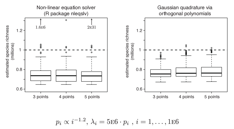
Figure S1: A comparison of directly solving the non-linear equations (4) with a non-linear equation solver Hasselman (2018) and via orthogonal polynomials. We simulated 100 samples from a power-law population and applied both algorithms using the same counts.

The current state of the art algorithms for computing Gaussian quadrature rules involve estimating the orthogonal polynomials associated with the underlying measure. We have found that this results in more stable estimates than with non-linear equation solvers (Figure S1).

Below we will present the theory specific to our problem needed to construct efficient algorithms based on Gaussian quadrature. For readers interested in a more in-depth explanation, we suggest the extensive textbooks of Gautschi (2004) or Golub and Meurant (2010).

Associated with every measure is a unique system of monic polynomials $\{p_{m}(\lambda);p_{m}(\lambda)=\lambda^{m}+\ldots,\,m=0,\ldots\}$ that are mutually orthogonal under the measure $\nu$, i.e. $\int_{0}^{\infty}p_{i}(\lambda)p_{m}(\lambda)d\nu(\lambda)$ is zero when $i\neq m$ and strictly positive when $i=m$. These orthogonal polynomials satisfy a three term recurrence

$$p_{m+1}(\lambda)=(\lambda-\alpha_{m})p_{m}(\lambda)-\beta_{m}p_{m-1}(\lambda),$$ (6)

$$\text{for }\alpha_{m},\beta_{m}>0\text{ and }p_{-1}(\lambda)=0,\,p_{0}(\lambda)=1.$$

The coefficients $\{\alpha_{m},\beta_{m}\}_{m\geq 0}$ define the orthogonal polynomials and are important because of a relationship between the coefficients of the three term recurrence and the points and weights that solve the system of equations (4).

Given the three term recurrence coefficients, define the Jacobi matrix to be the tridiagonal matrix with $\alpha_{m}$ on the diagonals and $\sqrt{\beta_{m}}$ on the off-diagonals. The truncated Jacobi matrix $J_{P}$ is the $P\times P$ matrix

$$\begin{pmatrix}\alpha_{0}&\sqrt{\beta_{1}}&0&\ldots&0\\ \sqrt{\beta_{1}}&\alpha_{1}&\sqrt{\beta_{2}}&\ldots&0\\ \vdots&&&\ddots&\vdots\\ 0&&\ddots&\alpha_{P-2}&\sqrt{\beta_{P-1}}\\ 0&&\ldots&\sqrt{\beta_{P-1}}&\alpha_{P-1}\end{pmatrix}.$$

The quadrature points $\psi_{1},\ldots,\psi_{P}$ are the eigenvalues of $J_{P}$ and quadrature weights are the square of the first component of the eigenvectors (Golub and Welsch, 1969). Given the estimated three term recurrence coefficients, these can be efficiently calculated with a modified QR algorithm that has complexity that is linear in both space and time. This is because since $J_{P}$ is already tridiagonal, the usual Householder transformations are not needed and we need only the first entry of the eigenvectors. Thus, it’s not necessary to store the full eigenvectors. Furthermore, this algorithm is perfectly conditioned, meaning that small changes in the estimated three term recurrence coefficients will not lead to large changes in the estimated quadrature points and weights.

0:  Estimated moments, $\{\hat{\nu}_{m},m=0,1,\ldots,2P-1\}$, of an unknown measure $\nu$.

0:  Estimated three term recurrence $\alpha_{0},\ldots,\alpha_{P-1}$ and $\beta_{1},\ldots,\beta_{P-1}$.

1:  $\alpha_{0}\leftarrow 1+\hat{\nu}_{1}/\hat{\nu}_{0}$,

2:  $\beta_{0}\leftarrow\hat{\nu}_{0}$

3:  for $l=1,2,\ldots,2P-2$ do

4:     $\sigma_{-1,l}\leftarrow 0$

5:     for $l=0,1,\ldots,2P-1$ do

6:        $\sigma_{0,l}\leftarrow\hat{\nu}_{l}$

7:     end for

8:  end for

9:  for $k=1,\ldots,P-1$ do

10:     for $l=k,k+1,\ldots,2P-k-1$ do

11:        $\sigma_{k,l}\leftarrow\sigma_{k-1,l+1}-\alpha_{k-1}\sigma_{k-1,l}-\beta_{k-1}\sigma_{k-2,l}$

12:     end for

13:     $\alpha_{k}\leftarrow\frac{\sigma_{k,k+1}}{\sigma_{k,k}}-\frac{\sigma_{k-1,k}}{\sigma_{k-1,l-1}}$

14:     $\beta_{k}\leftarrow\frac{\sigma_{k,k}}{\sigma_{k-1,k-1}}$

15:  end for

Algorithm 1 The unmodified Chebyshev algorithm

On the other hand, the three term recurrence coefficients can be written as functions of determinants of matrices that are structurally similar to the moment Hankel matrices (full details can be found in (Gautschi, 2004, Chapter 2)). These matrices have absolute condition number that grow exponentially in $P$ (Gautschi, 1982; Tyrtyshnikov, 1994), and therefore estimating the three term recurrence coefficients is extremely ill-conditioned. In our problem we do not have the expected moments, instead only noisy estimates of the moments. A consequence of the ill-conditioning issue is that due to errors in estimating the moments, we may have difficulties in accurately estimating the quadrature points. This is particularly difficult for the smallest point, which has largest effect on the estimated number of missing species.

The standard algorithm for calculating the three term recurrence of the orthogonal polynomials using only moment information is the modified Chebyshev algorithm (Gautschi, 2004), originally developed by Sack and Donovan (1971). The modified Chebyshev algorithm uses a known measure with an analytically derived three term recurrence to help condition the unknown measure and requires $O(P^{2})$ computations, rather than $O(P^{3})$ required from direct computation from the determinant relations. As we mentioned previously, the map from the moments to the recurrence coefficients of the orthogonal polynomials is ill-conditioned and the hope in using the modified Chebyshev is that a good choice of the modifying measure will improve the conditioning of the algorithm and improve estimation (Gautschi, 1985). For example, if the known measure is serendipitously chosen to be unknown measure then the measure is perfectly recovered. We previously (Daley, 2014) investigated a case where the true measure is known and the recurrence coefficients can be calculated analytically, specifically when $\mu$ is a Gamma distribution and the counts are Negative Binomial. We found that in the presence of error, the modified Chebyshev algorithm does not improve performance. We found instead that the use of no conditioning measure performs the best in our problem. Using no modifying measure results in what is known as the unmodified Chebyshev and is described in algorithm 1. This uses only the observed moments as input and requires no other input from the user to calculate the estimated recurrence relation, and to subsequently calculate the quadrature rules.

4 Evaluation on discrete distributions

We evaluated our moment-based estimator first on the simplest case of heterogeneity in the abundance distribution, discrete mixtures. For this initial comparison, we tested our method (preseq) against the Chao estimator (chao; Chao, 1984), the non-parametric maximum likelihood estimator (npmle; Norris and Pollock, 1998), and the penalized non-parametric maximum likelihood estimator (pnpmle; Wang and Lindsay, 2005). We use the implementations of the above algorithms available in the R package SPECIES (Wang, 2011), with the bootstrap option turned off. For all of the below simulations, the total number of species is $S=$1,000,000.

We measured the performance of the estimators in multiple ways. It is important that the estimator is close on average, which we measure by the median. The median ignores the variability of the estimator, so we used the root mean square error (RMSE) to measure the bias-variance tradeoff of the estimators. Since our simulated populations are orders of magnitude larger than populations previously investigated, we also measured the running time of the algorithms. Finally, for the preseq, npmle, and pnpmle methods, we kept track of the number of times the methods selected the correct number of components in the mixture to measure the ability of the algorithms to choose the correct model.

4.1 Two component mixture abundance distributions

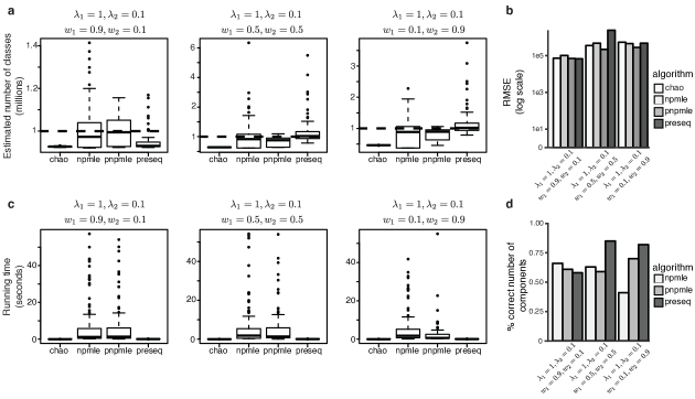
Figure 1: Comparison of chao, npmle, pnpmle, and preseq estimators for the total number of classes when the underlying population follows a 2-component discrete distribution. There are three cases: $\lambda_{1}=1,\lambda_{2}=0.1$ and $\pi_{1}=0.9,\pi_{2}=0.1$; $\lambda_{1}=1,\lambda_{2}=0.1$ and $\pi_{1}=0.5,\pi_{2}=0.5$; and $\lambda_{1}=1,\lambda_{2}=0.1$ and $\pi_{1}=0.1,\pi_{2}=0.9$. a Boxplots of the estimated number of classes. b Root mean square error (RMSE) of the estimators. c Boxplot of the running times. d The percentage of times the npmle, the pnpmle, and preseq chose the correct number of components in the underlying mixture.

For the two component mixture we considered three basic cases: the more abundant classes make up a majority of the population ($\lambda_{1}=1,\lambda_{2}=0.1$ and $\pi_{1}=0.9,\pi_{2}=0.1$); the population is nearly equally split between a low abundance portion and a high abundance portion ($\lambda_{1}=1,\lambda_{2}=0.1$ and $\pi_{1}=0.5,\pi_{2}=0.5$); and the least abundant classes make up a majority of the population ($\lambda_{1}=1,\lambda_{2}=0.1$ and $\pi_{1}=0.1,\pi_{2}=0.9$).

Figure 1 shows the comparison of the estimators. We note several things, in the latter two cases the median of the preseq estimates is very close to the true number of classes but the RMSE is very high. This is because in a few number of cases preseq vastly overestimates the number of unobserved classes, indicating that the ill-conditioning of the estimator is a problem. We will discuss a bootstrapping strategy to deal with this issue in the next section. In the first case, the median of the pnpmle estimates is closest to the true number of classes but preseq has the lowest RMSE. To achieve a low RMSE, it may be a viable strategy to consistently underestimate the number of classes to decrease the variance of the estimator. We see this in the first case studied. The preseq estimator choose 2 components in 63 out of the 100 simulations, and defaulted to the chao estimator in the other 37 simulation.

One very noticeable difference between the estimators is the running time. The chao estimator will of course be very fast to compute, but there is a dramatic difference in running time between the moment-based estimators and the maximum likelihood-based estimators. The large running time of the maximum likelihood-based methods will make it difficult to construct efficient bootstrap-aggregated estimators. On the other hand, it will be quite easy to construct bootstrap-aggregated estimators for the moment-based estimators.

4.2 Three component mixture abundance distributions

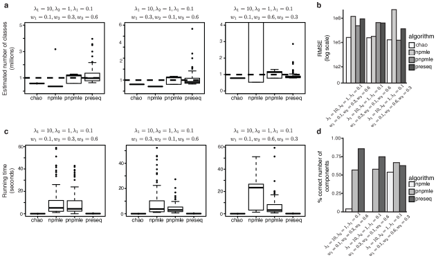
Figure 2: Comparison of chao, npmle, pnpmle, and preseq estimators for the total number of classes when the underlying population follows a 3-component discrete distribution. We considered three cases: $\lambda_{1}=10,\lambda_{2}=1,\lambda_{3}=0.1$ and $\pi_{1}=0.1,\pi_{2}=0.3,\pi_{3}=0.6$; $\lambda_{1}=10,\lambda_{2}=1,\lambda_{3}=0.1$ and $\pi_{1}=0.3,\pi_{2}=0.1,\pi_{3}=0.6$; and $\lambda_{1}=10,\lambda_{2}=1,\lambda_{3}=0.1$ and $\pi_{1}=0.1,\pi_{2}=0.6,\pi_{3}=0.3$. a Boxplots of the estimated number of classes. b Root mean square error (RMSE) of the estimators. c Boxplot of the running times. d The percentage of times the npmle, the pnpmle, and preseq chose the correct number of components in the underlying mixture.

With a three component mixture, there are many cases we could possibly consider. We focus on the following three cases: $\lambda_{1}=10,\lambda_{2}=1,\lambda_{3}=0.1$ and $\pi_{1}=0.1,\pi_{2}=0.3,\pi_{3}=0.6$; $\lambda_{1}=10,\lambda_{2}=1,\lambda_{3}=0.1$ and $\pi_{1}=0.3,\pi_{2}=0.1,\pi_{3}=0.6$; and $\lambda_{1}=10,\lambda_{2}=1,\lambda_{3}=0.1$ and $\pi_{1}=0.1,\pi_{2}=0.6,\pi_{3}=0.3$.

Figure 2 shows the comparison of the estimators in the three 3-component cases considered. The median of the preseq estimates is the closest to the true number of classes. But what figure 2a is missing is that largest estimate from preseq is on the order of the hundreds of millions for all three cases. This problem is not unique to moment-based estimation, as the maximum of the pnpmle estimates is on the order of hundreds of millions in the first two cases and the maximum of the npmle estimates is on the order of billions in the first and last cases. In fact, in the last case the median of the npmle estimates is approximately 1.3 billion. This is why in all cases the chao estimator vastly outperforms all other methods in terms of RMSE.

To alleviate the issue of infrequently large estimates from an otherwise well performing estimator, which seems to be a common problem in species estimation, a bootstrap-aggregating (bagging) approach was proposed by Kuhnert et al. (2008). We will discuss such an approach for the moment-based estimator in the next section.

5 Bagging for more accurate estimates of the missing number of classes

Consider a full set of count frequencies $n_{0},n_{1},n_{2},\ldots$. The likelihood of this set is equal to

$$\binom{S}{n_{0},n_{1},\ldots}\prod_{j=0}^{\infty}(f_{j})^{n_{j}},$$

with $f_{j}=\int_{0}^{\infty}e^{-\lambda}\lambda^{j}/j!d\mu(\lambda)$. As usual (Sanathanan, 1972), we split the likelihood into two parts: the unobserved portion and the observed portion as follows,

$$\binom{S}{n_{0},n_{1},\ldots}\prod_{j=0}^{\infty}(f_{j})^{n_{j}} =\binom{S}{n_{0}}f_{0}^{n_{0}}(1-f_{0})^{S-n_{0}}\,\cdot\,\binom{D}{n_{1},n_{2},\ldots}\prod_{j=1}^{\infty}\bigg{(}\frac{f_{j}}{1-f_{0}}\bigg{)}^{n_{j}}$$

$$=L(n_{0})\cdot L(n_{1},n_{2},\ldots).$$ (7)

Note that the observed data only enters the likelihood above through the latter part $L(n_{1},n_{2},\ldots)$. This indicates that we can take bootstrapped samples as multinomial samples with size parameter $D$ and probabilities $n_{1}/D,n_{2}/D,\ldots$, rather than sampling and the individual level. This will speed up the bootstrapping tremendously, as the number of items to sample per bootstrap is $D$, rather than $N$, and it’s always the case that $D\leq N$.

To alleviate the problem of extreme estimates, we take the median of the bootstrap estimates as the bagged estimator.

6 Applications

It is difficult and expensive to construct real experiments where the underlying population is known. One example for capture-recapture experiments is Carothers (1973), where the author used a known population of taxicabs and simulated capture by recording observed registration numbers during a capture period. For the large populations we wish to study, such experiments would be exorbitantly expensive.

We instead take a simulation based approach, using theoretical models proposed for our applications. We examine two cases where the total number of species is of great interest:

• T-Cell Receptor (TCR) repertoire, which are subject to depletion due to infection and age, and we can estimate the effect age has on reducing TCR repertoire;

• the total number of genes present in a cell of a single cell RNA sequencing (scRNA-seq) experiment, as this indicates cell quality and can represent a batch effect that will bias analysis (Hicks et al., 2017).

For comparison, we applied our moment-based estimator along with several other non-parametric species richness estimators. Specifically we applied Chao’s original lower bound (Chao, 1984), the duplicate fraction-based estimator of Chao and Bunge (2002), the jackknife estimator (Burnham and Overton, 1978), the abundance coverage-based estimator (ACE) (Chao and Lee, 1992), the penalized non-parametric maximum likelihood estimator (Wang and Lindsay, 2005), and the ratio regression-based method of Willis and Bunge (2015). For the first five estimators we used the R package SPECIES (Wang, 2011). For the ratio regression estimator we used the R package breakaway.

6.1 TCR repertoire

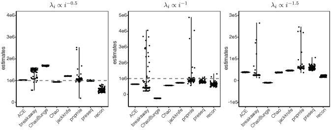
Figure 3: Violin plots of the estimated total size of the TCR repertoire based on 100 independent samples of approximately one million sampled T-Cell receptors for power law distributed abundances with parameter $\alpha=0.5,1,1.5$. Dashed line indicates the true size of the TCR repertoire. Some estimates are missing because they are out of the figure boundaries. See Supplementary Figure S2 for the estimates on the log scale.

Interrogations of TCR repertoire typically reveal a long tails of highly abundant and, at the same time, a large number of rare receptors, e.g. Table 1. This behavior is typical of power law distributions, and recent work has shown that competitive effect for TCR binding may explain this behavior (Desponds et al., 2016).

We took a theoretical population of one million TCRs, with abundances $\lambda_{i}\propto i^{-\alpha}$ for $i=1,\ldots,10^{6}$ and $\alpha=0.5,1,1.5$. We set the average number of total TCRs sampled equal to one million, i.e. $\sum_{i}\lambda_{i}=10^{6}$. We then sampled 100 independent samples and compared the estimates obtained from ACE, breakaway, ChaoBunge, jackknife, pnpmle, preseq, and recon, a new non-parametric estimator designed specifically for estimating TCR repertoire (Kaplinsky and Arnaout, 2016).

The results of these simulations are shown in Figure 3. In all three cases considered, preseq estimates were the closest to the true number of species on average, as well as the lowest RMSE of any estimator. This indicates that increased variance from using more moments is offset by increased accuracy, particularly compared to Chao’s lower bound. In the cases $\alpha=0.5$ and $\alpha=1$, preseq estimates are not a strict lower bound, as Chao’s estimates are, but we believe that the increased accuracy is beneficial enough to compensate for this drawback.

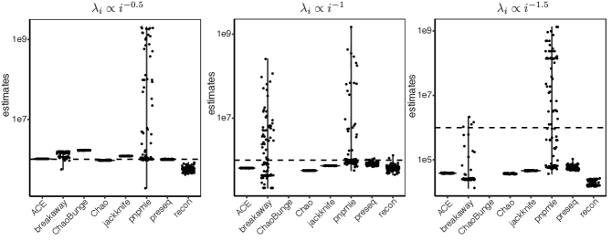
Figure S2: Violin plots of the estimated total size on the log scale of the TCR repertoire based on 100 independent samples of approximately one million sampled TCRs for power law distributed abundances with parameter $\alpha=0.5,1,1.5$. Dashed line indicates the true size of the TCR repertoire. Not shown are negative estimates, but these are shown in figure 3.

Some of the estimators, such as breakaway or pnpmle, had extremely large variation in their estimates, with estimates ranging over several orders of magnitude (Figure S2). This may be an indication that the models assumed by these estimators are not able to account for populations with long tailed abundances, typical of power-law distributions (Newman, 2005). Other estimators, such as ChaoBunge, had negative estimates, as others have previously found (Wang and Lindsay, 2005). This may indicate that the models these estimators use are not flexible enough to handle power law-like populations, despite their previous use in estimating TCR repertoire (Qi et al., 2014).

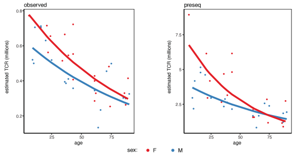
Figure 4: Estimated T-Cell repertoire as a function of age for the observed TCR and preseq estimates, along with estimated log-linear regressions for males and females subject separately.

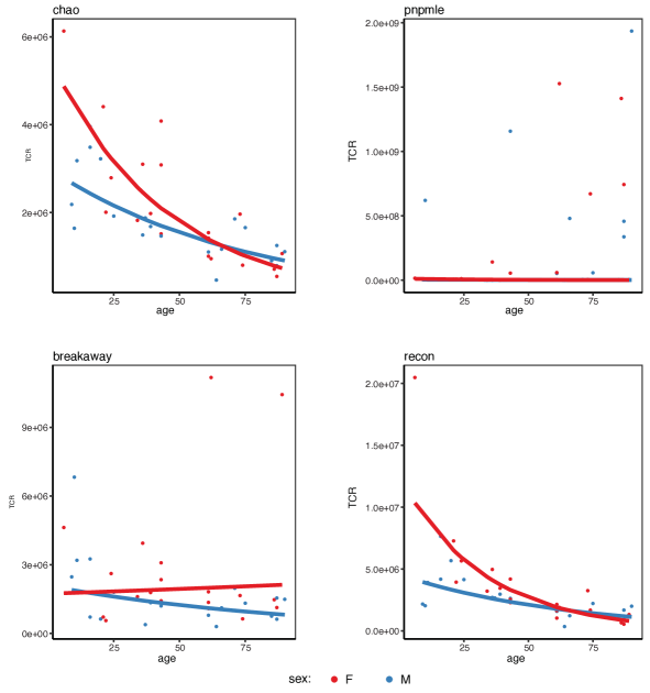
Figure S3: Estimated T-Cell repertoire as a function of age for the chao, pnpmle, breakaway, and recon estimates of TCR, along with estimated log-linear regressions for males and females subject separately.

Now we apply our method to real data from Britanova et al. (2014), looking at the decrease in T-Cell repertoire as a function of age. We assume that total TCR decreases exponentially with age, as a linear regression may result in negative estimates of the total repertoire. We compare female and male TCR as a function of age, looking at the original observations and the preseq missing species-corrected estimates, shown in Figure 4. Other estimators are show in Supplementary Figure S3. We see that after correction for the missing repertoire, female TCR is predicted to be lower on average than male TCR at around 75 years old. Without correction for the missing repertoire, the repertoire for females is not predicted to be lower than the male repertoire at any age considered. The consequence of lower T-Cell repertoire at advanced age is increased risk of infection (Yager et al., 2008; Blackman and Woodland, 2011), and such insights may guide decisions of treatment and outreach to prevent infections. We should note that the above is an example of exploratory analysis and a true test for the difference needs to take into account both the observed variance and variance from the estimated missing species (Willis et al., 2017).

6.2 Single cell RNA sequencing

Single-cell RNA sequencing (scRNAseq) is a new technology to interrogate the transcriptome of individual cells. Unfortunately, most assays can not capture the full transcriptome in an unbiased manner. Low abundant genes are more difficult to capture and are said to suffer from dropout when they are present in the original cell but are not captured by the assay (Hicks et al., 2017). These experiments also exhibit huge deviations from uniformity due to technical biases. It is therefore difficult to determine whether a gene is missing due to dropout or due to insufficient sequencing depth.

Estimating the dropout rate is critical to the normalization of scRNAseq data (Pierson and Yau, 2015; Lun et al., 2016) and is equivalent to estimating the number of genes that are present in the experiment but were not sampled due to insufficient sequencing depth. We can apply species sampling models to estimate the dropout rate. Our previous experience has shown the value in non-parametric models for sequencing experiments (Daley and Smith, 2013), so we will test our proposed estimator and other non-parametric estimators to the problem of estimating the dropout rate in simulated scRNAseq experiments.

We use the simulation framework of Lun et al. (2016), with some small modifications proposed by Hicks et al. (2017) to introduce batch-related dropout effects. We assume that we measured 20,000 genes in 1,000 captured cells. We assume that the population consists of two subpopulations, each making up half of the cells. These may represent different cell types or another biological condition. We assume that the count of gene $i$ in cell $j$ obtained from the scRNAseq experiment is a log-Normal-Poisson random variable with mean equal to $d\theta_{j}\lambda_{ij}$ times independent log normal random variables with parameters $\mu=-0.5$ and $\sigma=1$. We assume that $\theta_{j}$’s are independent log-normal random variables with parameters $\mu=-2.5^{2}/2$ and $\sigma=2.5$. We assume that $\lambda_{ij}=\lambda_{i0}\phi_{ij}$, $\lambda_{i0}\sim\text{Gamma}(0.1,0.1)$, $d=0.05$, and $\phi_{ij}$ is a sub-population specific value. We assume that for cells in the first sub-population $\phi_{ij}=1$ for all genes and that for cells in the second population $\phi_{ij}=5$ for $10\%$ of the genes, $\phi_{ij}=0.2$ for another $10\%$ of the genes, and $\phi_{ij}=1$ for the remainder. The former two sets of genes represent condition specific differentially expressed genes. These parameters were chosen to simulate the properties of droplet-based scRNAseq experiments, as these allow for more cells to be captured but tend to be sparser than microfluidic-based experiments.

Following the dropout model of Hicks et al. (2017), we assumed that counts dropout with a probability that is logistic function of the baseline, with batch specific baseline values. Specifically we assume that the baseline probability $1/(1+\exp(-\beta_{0ij}))$ follows a Beta$(2,8)$ for half the population and a Beta$(2,38)$ for the other half, independent of condition. The dropout probability is then equal to

$$p_{ij}=1/\big{(}1+\exp\big{(}-\beta_{0ij}-0.5(\theta_{j}\lambda_{ij}-\bar{\theta_{\cdot}\lambda_{\cdot\cdot}})\big{)}\big{)}.$$

This simulates the condition where the population was processed in two batches, each with a batch specific dropout rate. After standard filtering (at least 50 counts per cell, 10 counts per gene, and genes must appear in at least 3 cells), we obtained a counts matrix of 436 cells and 5,262 genes (full details can be found at https://github.com/timydaley/SingleCellWeights).

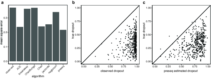
Figure 5: Estimating the number of unobserved genes improves dropout estimation. a Correlation of the corresponding estimated dropout rates to the true dropout rates. b Scatter plot of the observed dropout rate versus the true dropout rates. The dashed line indicates perfect estimation of the dropout rate. c Scatter plot of the preseq estimated dropout rates versus the true dropout rates. The other estimators are shown in Supplementary Fig S4. The improvement in estimation comes mostly from cells with high observed dropout.

The log-Normal Poisson is common for RNA-seq data, e.g. Jia et al. (2017), but initial tests indicate that the dropout and low sequencing depth of scRNA-seq experiments result in extremely high estimates of dropout (more than the number of genes). Accordingly, many groups have developed tools that extend models to account for dropout, e.g. Kharchenko et al. (2014) and Pierson and Yau (2015). Both of these do not allow for cell specific dropout rates, but recently researchers have recognized the need for estimating the dropout rate at the cell level (Risso et al., 2018). We investigated how non-parametric species estimation can improve the estimation of the dropout rate. We will use the same methods as in the previous section, excluding the pnmle and recon, as these methods are suitable for application to a single sample but take too long to apply to the number of number of samples (cells) obtained from a single cell RNA-seq experiment. We also added comparisons to a Negative Binomial parametric model, where the positive counts are assumed to arise from a zero-truncated Negative Binomial distribution. This represents a case where a close but incorrect parametric model is used. We used the EM algorithm available in the preseqR package (Deng et al., 2018) to fit the parameters of the Negative Binomial model. For methods that estimated a dropout rate less than zero, as occurs when the number of estimated genes is greater than the known number of genes, we set the dropout rate equal to the observed dropout rate.

Nearly all of the methods improve the estimated dropout rate (Fig 5a). The mean square error improved in all cases. The best performing methods in terms of lowest mean square error were the Chao lower bound, the ACE, and preseq (Fig 5a). All three improved the estimated dropout rate considerably better than all other tested methods, with preseq showing the highest performance. Most of the improvement was in the cells with very high observed dropout rates (Fig 5b and c). These cells present the most problems to investigators, as it is extremely unlikely that the observed sparse gene expression is due to biological factors.

method	$p_{\text{adj}}<0.01$	$p_{\text{adj}}<0.05$	$p_{\text{adj}}<0.1$
un-corrected	402	585	768
array weights	221	275	314
observation weights	162	256	345
preseq dropout	$\bm{643}$	$\bm{771}$	$\bm{771}$

Table 2: The number of genes correctly identified as differentially expressed with the correct sign at Bejamani-Hochberg adjusted $p=0.01,0.05,$ and $0.1$ for un-corrected, array weight-corrected, observation weights-corrected, and preseq dropout-corrected differential expression.

To illustrate the application of estimating the dropout to single cell RNA-seq, we use one minus the preseq-corrected dropout rate as cell weights in differential expression and show that this improves the performance of standard RNA-seq differential expression tools. The idea is that we want to up-weight cells that we trust more and down-weight cells that we trust less. Intuitively, we should trust cells with higher dropout less than we trust cells with a low dropout rate. If the differential expression is independent or orthogonal of the dropout rate, then this should improve the differential expression analysis. This is similar to the idea of using observation weights for scRNA-seq analysis presented in Van den Berge et al. (2018) but more akin to the approach presented by Liu et al. (2015), since the former weights every count individually and we are weighting the cells (i.e. samples). We applied this to the same data set as above, using edgeR/limma (Robinson et al., 2010; Ritchie et al., 2015) to compute differential expression. We used the preseq corrected dropout weights as input for the array weights in the standard pipeline. We compared the preseq corrected differential expression results to the uncorrected differential expression results, the array weights corrected differential expression results using the limma computed array weights, and differential expression results using observation weights from ZINB-WaVE (Risso et al., 2018). At B-H adjusted p-values of $0.01$, $0.05$, and $0.1$, the preseq corrected results identified the highest number of truly differentially expressed genes (Table 2, without a corresponding increase in the false positive rate (Fig S5).

These results indicate that the use of species estimation for cell-specific dropout correction can improve the analysis for differential expression analysis for single cell RNA-seq. Though a caveat must be made. If the conditions significantly differ in their dropout rates, possibly due to batch effects, then dropout correction may bias the differential expression analysis. This is something that the researcher should check early in the analysis, and it may indicate deeper problems with the data than can be corrected

7 Discussion

We presented a moment-based method for estimating the number of unobserved species in a large and heterogeneous population. This builds on the work of Harris (1959) and extends the estimator of Chao (1984) to modern large-scale sampling experiments, such as those that arise from high-throughput DNA sequencing. These experiments explore populations that are sizable and extremely diverse. To show highlight the performance of our estimator, we compared our method to other non-parametric estimators in two specific applications of species richness estimation in modern biology: T-Cell receptor repertoire and single-cell RNA-seq. We showed that in these two applications the use of our method can improve downstream inference.

We note one caveat of our method. Following the framework of Harris (1959), our method can be used to obtain bounds on a broad range of functionals of the abundance distribution. However, we believe that it should not be used to recover the abundance distribution. Methods such as the npmle (Norris and Pollock, 1998) or the pnpmle (Wang and Lindsay, 2005) are specifically designed for this task and should be used instead. Indeed, we think that this problem is much more difficult and one benefit of our method is the avoidance of this problem.

As we mentioned briefly in section 3, upper bounds for the number of species is infinite due to the inclusion of the boundary point 0 in the abundance distribution. If the abundance distribution is assumed to have a non-zero lower bound, then upper bounds can theoretically be obtained via Gaussian quadrature. Preliminary results indicate that the upper bounds are too large to be practically useful, hence our focus on lower bounds.

Our method is available in the open source package preseq (https://github.com/smithlabcode/preseq) under the bound_pop module.

Acknowledgements

The authors would like to thank Kristian Lum, Peter Calabrese, Manuel Lladser, Susan Holmes, James Johndrow, and especially Chao Deng for their helpful comments and discussion. Without their help this paper would be have been forever stuck in limbo.

Supplemental Figures

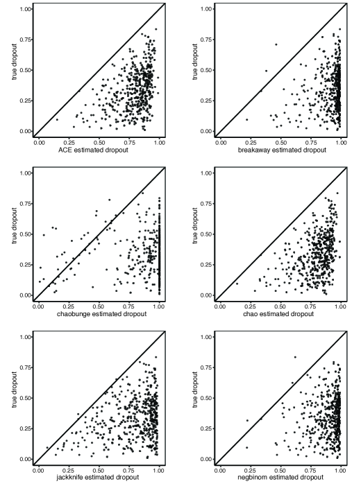
Figure S4: Plots of the estimated dropout versus the true dropout for the Chao, ACE, ChaoBunge, breakaway, and jackknife estimators, as described in Fig 5b and c.

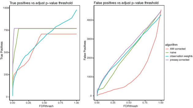
Figure S5: The number of true differentially expressed genes identified with the correct sign (left) out of a total of 1,167 truly differentially expressed genes and the number of incorrectly identified differentially expressed genes, either truly null or with the wrong sign, as a function of Benjamani-Hochberg corrected false discovery rate.

References

- Benjamini and Speed (2012) Benjamini, Y. and Speed, T. P. (2012). Summarizing and correcting the GC content bias in high-throughput sequencing. Nucleic acids research, page gks001.
- Blackman and Woodland (2011) Blackman, M. A. and Woodland, D. L. (2011). The narrowing of the CD8 T cell repertoire in old age. Current opinion in immunology, 23(4), 537–542.
- Böhning and Schön (2005) Böhning, D. and Schön, D. (2005). Nonparametric maximum likelihood estimation of population size based on the counting distribution. Journal of the Royal Statistical Society: Series C (Applied Statistics), 54(4), 721–737.
- Böhning et al. (2013) Böhning, D., Baksh, M. F., Lerdsuwansri, R., and Gallagher, J. (2013). Use of the ratio plot in capture–recapture estimation. Journal of Computational and Graphical Statistics, 22(1), 135–155.
- Britanova et al. (2014) Britanova, O. V., Putintseva, E. V., Shugay, M., Merzlyak, E. M., Turchaninova, M. A., Staroverov, D. B., Bolotin, D. A., Lukyanov, S., Bogdanova, E. A., Mamedov, I. Z., et al. (2014). Age-related decrease in TCR repertoire diversity measured with deep and normalized sequence profiling. The Journal of Immunology, 192(6), 2689–2698.
- Bunge and Fitzpatrick (1993) Bunge, J. and Fitzpatrick, M. (1993). Estimating the number of species: a review. Journal of the American Statistical Association, 88(421), 364–373.
- Bunge et al. (2014) Bunge, J., Willis, A., and Walsh, F. (2014). Estimating the number of species in microbial diversity studies. Annual Review of Statistics and Its Application, 1, 427–445.
- Burnham and Overton (1978) Burnham, K. P. and Overton, W. S. (1978). Estimation of the size of a closed population when capture probabilities vary among animals. Biometrika, 65(3), 625–633.
- Carothers (1973) Carothers, A. (1973). Capture-recapture methods applied to a population with known parameters. The Journal of Animal Ecology, pages 125–146.
- Chao (1977) Chao, A. (1977). The Quadrature Method in Inference Problems Arising from the Generalized Multinomial Distribution. Ph.D. thesis, University of Wisconsin-Madison.
- Chao (1984) Chao, A. (1984). Nonparametric estimation of the number of classes in a population. Scandinavian Journal of Statistics, pages 265–270.
- Chao and Bunge (2002) Chao, A. and Bunge, J. (2002). Estimating the number of species in a stochastic abundance model. Biometrics, 58(3), 531–539.
- Chao and Lee (1992) Chao, A. and Lee, S.-M. (1992). Estimating the number of classes via sample coverage. Journal of the American Statistical Association, 87(417), 210–217.
- Chiu et al. (2014) Chiu, C.-H., Wang, Y.-T., Walther, B. A., and Chao, A. (2014). An improved nonparametric lower bound of species richness via a modified Good–Turing frequency formula. Biometrics.
- Daley and Smith (2013) Daley, T. and Smith, A. D. (2013). Predicting the molecular complexity of sequencing libraries. Nature methods, 10(4), 325–327.
- Daley (2014) Daley, T. P. (2014). Non-Parametric Models for Large Capture-Recapture Experiments with Applications to DNA Sequencing. Ph.D. thesis, University of Southern California.
- Deng et al. (2018) Deng, C., Daley, T., and Smith, A. D. (2018). preseqR. package: Predicting r-species accumulation curves.
- Deng et al. (2019) Deng, C., Daley, T. P., Brandine, G. D. S., and Smith, A. D. (2019). Molecular heterogeneity in large-scale biological data: Techniques and applications. Annual Review of Biomedical Data Science, In Press.
- Desponds et al. (2016) Desponds, J., Mora, T., and Walczak, A. M. (2016). Fluctuating fitness shapes the clone-size distribution of immune repertoires. Proceedings of the National Academy of Sciences, 113(2), 274–279.
- Efron and Thisted (1976) Efron, B. and Thisted, R. (1976). Estimating the number of unseen species: How many words did Shakespeare know? Biometrika, 63(3), 435–447.
- Fisher et al. (1943) Fisher, R. A., Corbet, A. S., and Williams, C. B. (1943). The relation between the number of species and the number of individuals in a random sample of an animal population. The Journal of Animal Ecology, pages 42–58.
- Gautschi (1982) Gautschi, W. (1982). On generating orthogonal polynomials. SIAM Journal on Scientific and Statistical Computing, 3(3), 289–317.
- Gautschi (1983) Gautschi, W. (1983). How and how not to check Gaussian quadrature formulae. BIT Numerical Mathematics, 23(2), 209–216.
- Gautschi (1985) Gautschi, W. (1985). Orthogonal polynomials?constructive theory and applications. Journal of Computational and Applied Mathematics, 12, 61–76.
- Gautschi (2004) Gautschi, W. (2004). Orthogonal Polynomials: Computation and Approximation, Numerical Mathematics and Scientific Computation Series. Oxford University Press, Oxford.
- Golub and Meurant (2010) Golub, G. H. and Meurant, G. (2010). Matrices, moments and quadrature with applications. Princeton University Press.
- Golub and Welsch (1969) Golub, G. H. and Welsch, J. H. (1969). Calculation of Gauss quadrature rules. Mathematics of Computation, 23(106), 221–230.
- Gopalakrishnan et al. (2018) Gopalakrishnan, V., Spencer, C., Nezi, L., Reuben, A., Andrews, M., Karpinets, T., Prieto, P., Vicente, D., Hoffman, K., Wei, S., et al. (2018). Gut microbiome modulates response to anti–PD-1 immunotherapy in melanoma patients. Science, 359(6371), 97–103.
- Gravel (2014) Gravel, S. (2014). Predicting discovery rates of genomic features. Genetics, pages genetics–114.
- Haas et al. (1995) Haas, P. J., Naughton, J. F., Seshadri, S., and Stokes, L. (1995). Sampling-based estimation of the number of distinct values of an attribute. In Proceedings of the 21th International Conference on Very Large Data Bases, pages 311–322. Morgan Kaufmann Publishers Inc.
- Harris (1959) Harris, B. (1959). Determining bounds on integrals with applications to cataloging problems. The Annals of Mathematical Statistics, 30(2), 521–548.
- Hasselman (2018) Hasselman, B. (2018). Package nleqslv.
- Hicks et al. (2017) Hicks, S. C., Townes, F. W., Teng, M., and Irizarry, R. A. (2017). Missing data and technical variability in single-cell rna-sequencing experiments. bioRxiv, page 025528.
- Jia et al. (2017) Jia, C., Hu, Y., Kelly, D., Kim, J., Li, M., and Zhang, N. R. (2017). Accounting for technical noise in differential expression analysis of single-cell rna sequencing data. Nucleic Acids Research, 45(19), 10978–10988.
- Kaplinsky and Arnaout (2016) Kaplinsky, J. and Arnaout, R. (2016). Robust estimates of overall immune-repertoire diversity from high-throughput measurements on samples. Nature communications, 7.
- Karlin and Shapley (1953) Karlin, S. and Shapley, L. (1953). Geometry of moment spaces. American Mathematical Society.
- Karlin and Studden (1966) Karlin, S. and Studden, W. J. (1966). Tchebycheff Systems: With Applications in Analysis and Statistics, volume 376. Interscience Publishers New York.
- Kharchenko et al. (2014) Kharchenko, P. V., Silberstein, L., and Scadden, D. T. (2014). Bayesian approach to single-cell differential expression analysis. Nature methods, 11(7), 740–742.
- Kuhnert et al. (2008) Kuhnert, R., Del Rio Vilas, V. J., Gallagher, J., and Böhning, D. (2008). A bagging-based correction for the mixture model estimator of population size. Biometrical Journal, 50(6), 993–1005.
- Liu et al. (2015) Liu, R., Holik, A. Z., Su, S., Jansz, N., Chen, K., Leong, H. S., Blewitt, M. E., Asselin-Labat, M.-L., Smyth, G. K., and Ritchie, M. E. (2015). Why weight? modelling sample and observational level variability improves power in RNA-seq analyses. Nucleic acids research, 43(15), e97–e97.
- Lun et al. (2016) Lun, A. T., Bach, K., and Marioni, J. C. (2016). Pooling across cells to normalize single-cell rna sequencing data with many zero counts. Genome biology, 17(1), 75.
- Mao and Lindsay (2001) Mao, C. X. and Lindsay, B. G. (2001). Moment-based nonparametric estimators for the number of classes in a population.
- Mao and Lindsay (2007) Mao, C. X. and Lindsay, B. G. (2007). Estimating the number of classes. The Annals of Statistics, pages 917–930.
- Newman (2005) Newman, M. E. (2005). Power laws, pareto distributions and zipf’s law. Contemporary physics, 46(5), 323–351.
- Norris and Pollock (1998) Norris, J. L. and Pollock, K. H. (1998). Non-parametric MLE for Poisson species abundance models allowing for heterogeneity between species. Environmental and Ecological Statistics, 5(4), 391–402.
- Pierson and Yau (2015) Pierson, E. and Yau, C. (2015). Zifa: Dimensionality reduction for zero-inflated single-cell gene expression analysis. Genome biology, 16(1), 241.
- Pozza and Strakoš (2019) Pozza, S. and Strakoš, Z. (2019). Algebraic description of the finite stieltjes moment problem. Linear Algebra and its Applications, 561, 207–227.
- Qi et al. (2014) Qi, Q., Liu, Y., Cheng, Y., Glanville, J., Zhang, D., Lee, J.-Y., Olshen, R. A., Weyand, C. M., Boyd, S. D., and Goronzy, J. J. (2014). Diversity and clonal selection in the human T-cell repertoire. Proceedings of the National Academy of Sciences, 111(36), 13139–13144.
- Risso et al. (2018) Risso, D., Perraudeau, F., Gribkova, S., Dudoit, S., and Vert, J.-P. (2018). A general and flexible method for signal extraction from single-cell RNA-seq data. Nature communications, 9(1), 284.
- Ritchie et al. (2015) Ritchie, M. E., Phipson, B., Wu, D., Hu, Y., Law, C. W., Shi, W., and Smyth, G. K. (2015). limma powers differential expression analyses for RNA-sequencing and microarray studies. Nucleic acids research, 43(7), e47–e47.
- Robinson et al. (2010) Robinson, M. D., McCarthy, D. J., and Smyth, G. K. (2010). edgeR: a bioconductor package for differential expression analysis of digital gene expression data. Bioinformatics, 26(1), 139–140.
- Sack and Donovan (1971) Sack, R. and Donovan, A. (1971). An algorithm for Gaussian quadrature given modified moments. Numerische Mathematik, 18(5), 465–478.
- Sanathanan (1972) Sanathanan, L. (1972). Estimating the size of a multinomial population. The Annals of Mathematical Statistics, pages 142–152.
- Simon (1998) Simon, B. (1998). The classical moment problem as a self-adjoint finite difference operator. Advances in Mathematics, 137(1), 82–203.
- Sims et al. (2014) Sims, D., Sudbery, I., Ilott, N. E., Heger, A., and Ponting, C. P. (2014). Sequencing depth and coverage: key considerations in genomic analyses. Nature Reviews Genetics, 15(2), 121–132.
- Tyrtyshnikov (1994) Tyrtyshnikov, E. E. (1994). How bad are Hankel matrices? Numerische Mathematik, 67(2), 261–269.
- Van den Berge et al. (2018) Van den Berge, K., Perraudeau, F., Soneson, C., Love, M. I., Risso, D., Vert, J.-P., Robinson, M. D., Dudoit, S., and Clement, L. (2018). Observation weights unlock bulk RNA-seq tools for zero inflation and single-cell applications. Genome biology, 19(1), 24.
- Wang (2011) Wang, J.-P. (2011). SPECIES: an R package for species richness estimation. Journal of Statistical Software, 40(9), 1–15.
- Wang and Lindsay (2005) Wang, J.-P. Z. and Lindsay, B. G. (2005). A penalized nonparametric maximum likelihood approach to species richness estimation. Journal of the American Statistical Association, 100(471), 942–959.
- Willis and Bunge (2015) Willis, A. and Bunge, J. (2015). Estimating diversity via frequency ratios. Biometrics.
- Willis et al. (2017) Willis, A., Bunge, J., and Whitman, T. (2017). Improved detection of changes in species richness in high diversity microbial communities. Journal of the Royal Statistical Society: Series C (Applied Statistics), 66(5), 963–977.
- Yager et al. (2008) Yager, E. J., Ahmed, M., Lanzer, K., Randall, T. D., Woodland, D. L., and Blackman, M. A. (2008). Age-associated decline in T cell repertoire diversity leads to holes in the repertoire and impaired immunity to influenza virus. Journal of Experimental Medicine, 205(3), 711–723.