Capacity of Three-Dimensional Erasure Networks

Abstract

In this paper, we introduce a large-scale three-dimensional (3D) erasure network, where $n$ wireless nodes are randomly distributed in a cuboid of $n^{\lambda}\times n^{\mu}\times n^{\nu}$ with $\lambda+\mu+\nu=1$ for $\lambda,\mu,\nu>0$, and completely characterize its capacity scaling laws. Two fundamental path-loss attenuation models (i.e., exponential and polynomial power-law models) are used to suitably model an erasure probability for packet transmission. Then, under the two erasure models, we introduce a routing protocol using percolation highway in 3D space, and then analyze its achievable throughput scaling laws. It is shown that, under the two erasure models, the aggregate throughput scaling $n^{\operatornamewithlimits{min}\{1-\lambda,1-\mu,1-\nu\}}$ can be achieved in the 3D erasure network. This implies that the aggregate throughput scaling $n^{2/3}$ can be achieved in 3D cubic erasure networks while $\sqrt{n}$ can be achieved in two-dimensional (2D) square erasure networks. The gain comes from the fact that, compared to 2D space, more geographic diversity can be exploited via 3D space, which means that generating more simultaneous percolation highways is possible. In addition, cut-set upper bounds on the capacity scaling are derived to verify that the achievable scheme based on the 3D percolation highway is order-optimal within a polylogarithmic factor under certain practical operating regimes on the decay parameters.

I Introduction

he Internet evolves into the next phase: the network consisting of smart devices equipped with sensors and radio frequency transceivers, connected to the Internet for sharing information with each other, which is known as the Internet of Things (IoT). Such smart devices are used for smart home, smart building, smart metering, etc. For example, home appliances are connected to wireless networks so that a user controls its home appliances remotely. In a smart building, heating, ventilation, air conditioning, and lighting are automatically controlled. Utilizing a smart metering where utility meters such as electricity, water, and gas are reported to the data center, not only customers can save energy but also energy suppliers can help better serve their customers. Machine-to-machine (M2M) or machine-type communications [1] has recently received a lot of attention as an enabling technology of IoT. As a massive number of devices participate in M2M communications, a study on the capacity scaling law has been taken into account as one of the most challenging issues in understanding a fundamental limit on the network throughput and its asymptotic trend with respect to the number of devices. One can obtain remarkable insights into the practical design of a protocol by characterizing such a capacity scaling behavior.

I-A Previous Work

In [2], the throughput scaling for Gaussian channels was originally introduced and characterized in a large wireless ad hoc network where nodes are distributed in two-dimensional (2D) space. It was shown that the aggregate throughput scales as $\Theta(\sqrt{n/\operatorname{log}n})$ in a network having $n$ nodes randomly distributed in a unit area. This throughput scaling is achieved using the nearest-neighbor multihop (MH) routing scheme (also known as the Gupta–Kumar routing scheme). MH schemes were further studied and analyzed in [4, 5, 6, 7, 8, 9]. In [4], the aggregate throughput scaling was improved to $\Theta(\sqrt{n})$ using percolation theory, which newly models the connectivity of wireless networks. It was shown that a hierarchical cooperation (HC) strategy [10, 11, 12] achieves an almost linear throughput scaling, i.e., $\Theta(n^{1-\epsilon})$ for an arbitrarily small $\epsilon>0$, in the Gaussian network model. In addition, in Gaussian networks of unit area, there has been a lot of research to improve the aggregate throughput up to a linear scaling by using novel techniques such as networks with node mobility [13], interference alignment [14], directional antennas [15, 16, 17], and infrastructure support [18, 19, 20, 21, 22, 23, 24].

The aforementioned studies focused only on 2D wireless networks. In cities such as Manhattan, where there exist a number of skylines, however, all kinds of nodes such as sensors, meters, appliances, and traffic lights can be located in three-dimensional (3D) space. Hence, in such a scenario, assuming a 3D network is rather suitable. A large-scale, low-cost wireless sensor network testbed was deployed in Singapore and the inter-floor connectivity was tested [25]. The Zigbee-based IoT was investigated in 3D terrains [26]. It is thus envisioned that 3D wireless networks will receive much more attention in M2M communications. In 3D Gaussian networks, there have been a few studies in the literature [27, 28, 29, 30] regarding the throughput scaling analysis. In [27], the capacity was analyzed under both Protocol and Physical Models when $n$ nodes are distributed in a sphere. A more general physical model was employed in [28] to better characterize the throughput from an information-theoretic point of view. In [29], it was shown that per-node throughput scales as $O((\operatorname{log}n)^{3}/n^{1/3})$ using Maxwell’s physics of wave propagation in a 3D network where nodes are located inside a sphere. Similarly as in the 2D network scenario [4], per-node throughput scaling of $\Omega(1/n^{1/3})$ was shown to be achieved using percolation theory in a cubic network [30].

Besides the Gaussian channel setup, another fundamental class of channel models is an erasure network, originally introduced in [31], where signals are either successfully delivered or completely lost. This erasure channel model is well suited for packetized systems where all information in a packet may be lost due to the errors. The erasure channel plays an important role in information theory and coding theory [32, 33]. This is because, by modelling each communication channel in wireless networks as a memoryless erasure channel, one can easily tackle a long-standing open problem, corresponding to the capacity region for general Gaussian multiterminal networks (see [34, 35] and references therein). In large-scale wireless networks, the erasure probability will increase as the physical distance between one transmitter and its intended receiver increases since the link quality between the two nodes is degraded with distance. To incorporate this phenomenon into the erasure channel model, one can use either an exponential or polynomial decay model in computing the path-loss attenuation. In 2D erasure networks, the capacity scaling law was studied under the exponential decay model [36, 37], while the results in [38, 39, 40] assumed the polynomial power-law model in analyzing the capacity scaling law.

In [31], it was shown that network coding at intermediate nodes is needed to achieve the capacity region in a wireless erasure network, where each node transmits linear combinations of the received non-erased symbols. However, network coding does not further improve the throughput performance in large-scale networks as long as scaling laws are concerned [39, 41]. In other words, MH routing, which is a simple packet-forwarding scheme, is order-optimal in large-scale erasure networks. In [41], the benefits of feedback were also demonstrated, thereby allowing an extremely simple coding scheme. In contrast to the network coding in [31], a simple acknowledgement-based feedback from the destination enables us to eliminate the requirement for sending any side information including the erased locations in a packet [41]. Adding such a feedback, however, does not fundamentally change the throughput scaling law, compared to the case where no feedback is allowed.

I-B Contributions

In this paper, we introduce a general erasure network in 3D space, where $n$ wireless ad hoc nodes are randomly distributed in a cuboid of $n^{\lambda}\times n^{\mu}\times n^{\nu}$ with $\lambda+\mu+\nu=1$ having unit node density for $\lambda,\mu,\nu>0$. We also completely characterize its capacity scaling laws. In the Gaussian channel model, both upper and lower bounds on the capacity were shown in a 3D cubic network [28], but it still remains open how to further bridge the gap between the two bounds and then how to characterize the capacity scaling. To the best of our knowledge, the information-theoretic capacity scaling has never been analyzed before for 3D erasure networks.

We start by introducing two fundamental path-loss attenuation models (i.e., exponential and polynomial power-laws) to suitably model an erasure probability for packet transmission. As in [36, 39], inspired by the Physical model [2] under wireless Gaussian networks, we use the finite-field additive interference model in erasure networks. A percolation highway in 3D space is then introduced to analyze our achievable throughput scaling laws under the two practical erasure models. Specifically, a highway system consisting of percolation highways in horizontal and vertical directions over 2D networks is extended to the 3D network configuration where there exist percolation highways in three Cartesian directions. It is shown that, under both erasure models, the aggregate throughput scaling $n^{\operatornamewithlimits{min}\{1-\lambda,1-\mu,1-\nu\}}$ can be achieved. This result reveals that, in a cubic network (i.e., $\lambda=\mu=\nu=\frac{1}{3}$), the aggregate throughput scaling $\Omega(n^{2/3})$ can be achieved under both erasure models. We explicitly show how to operate our percolation-based highway routing based on a time-division multiple access (TDMA) scheme, which is not straightforward since finding the appropriate number of required time slots is essential for obtaining the above scaling result. We remark that this scaling is greater than the aggregate throughput scaling $\Omega(\sqrt{n})$ achievable in 2D square erasure networks. This is because, compared to 2D space, more geographic diversity can be exploited via 3D geolocation, which indicates that constructing more simultaneous end-to-end percolation highways is possible. In addition, to verify the optimality of the achievable scheme, we derive upper bounds on the capacity scaling for each path-loss attenuation model by using the max-flow min-cut theorem. It is shown that our upper bound matches the achievable throughput scaling within a polylogarithmic factor for all operating regimes under the exponential decay model and for $\alpha>3$ under the polynomial decay model, where $\alpha$ is the decay parameter for the polynomial decay model. The capacity scaling law in a 3D erasure network of unit volume (i.e., a dense network model) is also characterized.

Our main contributions are threefold as follows:

• We introduce a generalized 3D erasure network whose size is $n^{\lambda}\times n^{\mu}\times n^{\nu}$ with $\lambda+\mu+\nu=1$ and propose a constructive achievable scheme, i.e., a percolation-based 3D highway routing.

• We explicitly show our TDMA scheme by deriving the minimum number of required time slots to achieve the order optimality.

• We derive cut-set upper bounds on the capacity scaling, where both upper and lower bounds are of the same order within a polylogarithmic factor under a certain condition.

I-C Organization

The rest of this paper is organized as follows. In Section II, the system and channel models are described. The routing protocol based on percolation highways is presented in Section III. Achievable throughput scaling laws are derived for both exponential and polynomial decay models in Section IV. Cut-set upper bounds on the capacity scaling are then derived in Section V. Extension to the dense network scenario is discussed in Section VI. Finally, we summarize the paper with some concluding remark in Section VII.

II System and Channel Models

Consider a 3D wireless network where $n$ wireless nodes are uniformly and independently distributed in a cuboid of $n^{\lambda}\times n^{\mu}\times n^{\nu}$ with $\lambda+\mu+\nu=1$ having unit node density for $\lambda,\mu,\nu>0$ (i.e., an extended network [4, 10]). We randomly pick source–destination pairings so that each node is the destination of exactly one source.

The channel between any two nodes is modelled as a memoryless erasure channel with erasure events over all channels being independent. We consider two models of erasure probability $\epsilon_{ki}$ between nodes $i$ and $k$: the exponential decay model [36, 37] and the polynomial decay model [39, 40]. In the exponential decay model such that the probability of successful transmission decays exponentially with a distance between two nodes, it follows that

$$\epsilon_{ki}=1-\gamma^{d_{ki}},$$ (1)

where $0<\gamma<1$ is the decay parameter for the exponential decay model and $d_{ki}$ is the distance between nodes $i$ and $k$. As another important model, the erasure probability can be modeled as a polynomial power-law model in which the probability of successful transmission decays polynomially with a distance between two nodes. In this case, the erasure probability is given by

$$\epsilon_{ki}=1-\frac{1}{d_{ki}^{\alpha}},$$ (2)

where $\alpha>0$ is the decay parameter for the polynomial decay model.

Due to the broadcast nature of the wireless medium, under the finite-field additive interference model [36, 39], the received symbol at node $k$ is given by

$$y_{k}=\sum_{i\in\mathcal{I}}\eta_{ki}x_{i},$$

where $\mathcal{I}$ is the set of simultaneously transmitting nodes, $\eta_{ki}$ is a Bernoulli random variable that takes the value $0$ with probability $\epsilon_{ki}$ or $1$ with probability $1-\epsilon_{ki}$, and $x_{i}$ is a single symbol chosen at node $i$ from the finite-field alphabet $\mathcal{X}$. The output $y_{k}$ is the sum of all unerased symbols. It is assumed that each erased packet does not contribute to any interference since the packet can be successfully decoded due to the long packet length and robust channel coding if the received signal power is sufficiently high.

If a packet is erased at a certain receiver, then it will be retransmitted from the receiver to the desired transmitter to ensure the successful packet delivery based on the acknowledgements of an automatic repeat request (ARQ) protocol. For analytical convenience, we do not incorporate such a feedback mechanism into our setting since it does not fundamentally affect the achievability results as long as scaling laws are concerned.

III Routing Protocol

It was shown that the nearest-neighbor MH routing is order-optimal under the polynomial decay model in 2D erasure networks [39]. On the other hand, the nearest-neighbor MH routing is not sufficient in achieving the optimal capacity under the exponential decay model since the probability of successful transmission decreases exponentially in distance $d_{ki}$ between two nodes while per-hop distance (i.e., the distance between nodes in adjacent routing cells) increases logarithmically, thus resulting in a huge throughput degradation. Alternatively, in [36], the percolation-based routing was applied under the exponential decay model. In our 3D erasure network setup, we also introduce a routing protocol based on the 3D percolation highway for both polynomial and exponential decay models.

III-A Review on Percolation-Based Highway Routing

The routing protocol based on the percolation model [4] is briefly reviewed. When water percolates through one stone, the stone can be modelled as a square grid, in which each edge is open with probability $p$ and traversed by the water and is closed otherwise. A wireless ad hoc network can also be modelled in a similar fashion. A grid edge is open when there exists at least one wireless transmitter(s) in the position corresponding to the edge. Otherwise, it is closed. The open percolating paths can be treated as a wireless backbone, named a highway system, that conveys data packets across the network. The source nodes access the highway system using single-hop transmission, and then the information is carried via MH transmission using the highway system across the network.

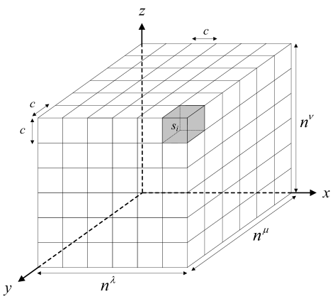
Figure 1: The tessellation of a cuboid network.

III-B Highway System

Let us introduce a highway system in our 3D network. As illustrated in Fig. 1, the cuboid is partitioned into subcubes $s_{i}$ of constant side length $c>0$, independent of $n$. Let $X(s_{i})$ denote the number of nodes inside $s_{i}$, which follows the binomial distribution with parameters $n$ and $\frac{c^{3}}{n}$. For the situation in which $n$ is large, the binomial distribution can be well-approximated by a Poisson distribution with parameter $c^{3}$. Thus, similarly as in [4, 8, 10, 24], the probability that a subcube contains at least one node is given by

$$p:=\Pr\{X(s_{i})\geq 1\}\mathop{\approx}\limits_{n\to\infty}1-e^{-c^{3}}.$$

We call that a subcube is open if it contains at least one node, and is closed otherwise. Then, the subcube is open with probability $p$, or is closed with probability $1-p$.

Let us consider a cuboid of side length $n^{\lambda}\times c\times n^{\nu}$, where a $y$-coordinate lies between $(i-1)c$ and $ic$ for an integer $i$ (refer to the left-hand side of Fig. 2). A vertical section $V_{xz}$ that cuts $\frac{n^{\lambda}}{c}\times\frac{n^{\nu}}{c}$ subcubes in the cuboid along the $x$-$z$ plane is depicted in the right-hand side of Fig. 2. The section $V_{xz}$ is tessellated into subsquares formed by projecting these subcubes onto $V_{xz}$. We associate an edge to each square, traversing it diagonally. An associated edge in the square lattice is called open if the corresponding subcube contains at least one node, and is closed otherwise. Each edge is open with probability $p$, independently of each other. A path is formed by connecting open edges, which are associated to subcubes that contain at least one node.

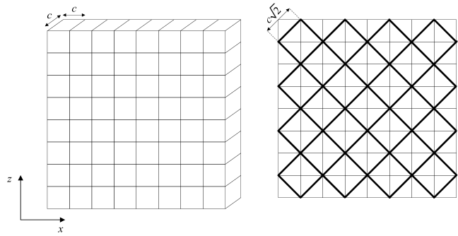
Figure 2: The construction of the percolation model along the $x$-$z$ plane.

Let us denote the number of subcubes in $x$, $y$, and $z$ directions by $m_{x}$, $m_{y}$, and $m_{z}$, respectively. Then, it follows that $m_{x}=\frac{n^{\lambda}}{c}$, $m_{y}=\frac{n^{\mu}}{c}$, and $m_{z}=\frac{n^{\nu}}{c}$. Now, as illustrated in Fig. 3, let us partition $V_{xz}$ into rectangles $R_{xz,x}^{j}$ of sides $m_{x}c\times c(\kappa\operatorname{log}m_{z}-\epsilon_{m})$, where $\kappa>0$ is an arbitrary constant and $\epsilon_{m}>0$ is chosen as the smallest value such that the number of rectangles in $V_{xz}$, $\frac{m_{z}}{\kappa\operatorname{log}m_{z}-\epsilon_{m}}$, is a positive integer. Similarly, $V_{xz}$ can be partitioned into rectangles $R_{xz,z}^{j}$ of sides $c(\kappa\operatorname{log}m_{x}-\epsilon_{m})\times m_{z}c$, where $\epsilon_{m}>0$ is chosen as the smallest value such that the number of rectangles in $V_{xz}$, $\frac{m_{x}}{\kappa\operatorname{log}m_{x}-\epsilon_{m}}$, is a positive integer. In the following lemma, it is shown that there are at least $\delta\operatorname{log}m_{z}$ paths crossing each rectangle $R_{xz,x}^{j}$ from left to right. It is also shown that there are at least $\delta\operatorname{log}m_{x}$ paths crossing each rectangle $R_{xz,z}^{j}$ from bottom to top.

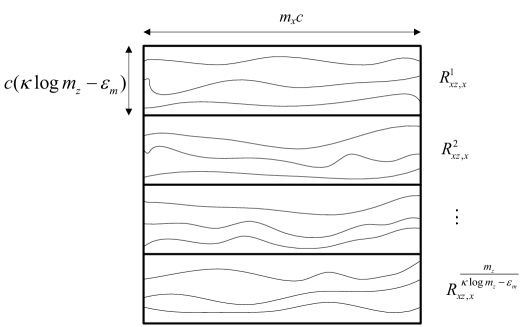
Figure 3: Many crossing paths that behave almost as straight lines from left to right.

Lemma 1

For all $\kappa>0$ and $\frac{5}{6}<p<1$ satisfying $1+\frac{\lambda}{\nu}+\kappa\operatorname{log}(6(1-p))<0$, there exists a $\delta>0$ such that

$$\lim_{n\rightarrow\infty}\Pr\{N_{xz,x}\leq\delta\operatorname{log}m_{z}\}=0,$$

where $N_{xz,x}=\operatornamewithlimits{min}_{j}C_{xz,x}^{j}$, $C_{xz,x}^{j}$ is the maximal number of edge-disjoint left-to-right crossings of rectangle $R_{xz,x}^{j}$, $j=1,\ldots,\frac{m_{z}}{\kappa\operatorname{log}m_{z}-\epsilon_{m}}$, and $m_{z}=\frac{n^{\nu}}{c}$. For all $\kappa>0$ and $\frac{5}{6}<p<1$ satisfying $1+\frac{\nu}{\lambda}+\kappa\operatorname{log}(6(1-p))<0$, there exists a $\delta>0$ such that

$$\lim_{n\rightarrow\infty}\Pr\{N_{xz,z}\leq\delta\operatorname{log}m_{x}\}=0,$$

where $N_{xz,z}=\operatornamewithlimits{min}_{j}C_{xz,z}^{j}$, $C_{xz,z}^{j}$ is the maximal number of edge-disjoint bottom-to-top crossings of rectangle $R_{xz,z}^{j}$, $j=1,\ldots,\frac{m_{x}}{\kappa\operatorname{log}m_{x}-\epsilon_{m}}$, and $m_{x}=\frac{n^{\lambda}}{c}$.

Proof:

Refer to Appendix A. ∎

Hence, if we select $p$ sufficiently large, then the percolation highways can be formed along $x$ and $z$ directions. The highways in $y$ direction can be formed by either the section $V_{xy}$ or $V_{yz}$. In what follows, it is assumed that the highways in $y$ direction are formed using horizontal paths in $V_{yz}$. Due to the symmetry of the $x$, $y$, and $z$ coordinates, as in Lemma 1, one can show that there also exist highways along $y$ direction. This constitutes our highway system in our cuboid network.

III-C Overall Procedure

Similarly as in  [30], the overall procedure of the routing protocol in our 3D network is described. Using the highway system in the network, the data packets can be delivered towards any direction in 3D space. The routing protocol under the 3D extended network consists of three phases and is explained as follows:

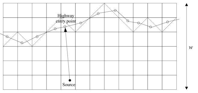
Figure 4: An illustration of the draining phase of the routing protocol.

• (Draining phase) The section $V_{xz}$ perpendicular to $y$-axis is sliced into horizontal strips of constant width $w$, independent of $n$, where we choose $w>0$ appropriately such that there are at least as many paths as slices inside each rectangle and thus $w=\Theta(1)$. By imposing that nodes in the $i$th slice use the $i$th horizontal path for packet delivery, the traffic can evenly be distributed into all highways in a rectangle. Each source in the $i$th slice transmits its data packets to the entry point on the $i$th path in $x$ direction, where the entry point is the node on the path closest to the vertical line drawn from the source node, as illustrated in Fig. 4.

• ($x$-highway phase) The packets are delivered along the highways in $x$ direction using MH routing until they reach the interchange point closest to the target highway in $y$ direction.

• (First highway interchange step) The packets are then delivered from the interchange point on the path in $x$ direction to another interchange point on a path in $y$ direction using single-hop, which is referred to as the first highway interchange step as illustrated in Fig. 5.

• ($y$-highway phase) The packets are delivered along the highways in $y$ direction using MH routing until they reach the interchange point closest to the target highway in $z$ direction.

• (Second highway interchange step) The packets are then delivered from the interchange point on the path in $y$ direction to another interchange point on a path in $z$ direction using single-hop, which is referred to as the second highway interchange step as illustrated in Fig. 5.

• ($z$-highway phase) The packets are delivered along the highways in $z$ direction using MH routing until they reach the exit point to the destination.

• (Delivery phase) The section $V_{xz}$ perpendicular to $y$-axis is sliced into vertical strips of constant width $w>0$ as in the draining phase. The packets are delivered from the exit point to the destination, where the exit point is the node on the path in $z$ direction closest to the horizontal line drawn from the destination.

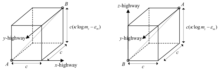
Figure 5: An illustration of the highway interchange phase of the routing protocol. In the left figure, the packets on the highway in $x$ direction are delivered to the highway in $y$ direction. In the right figure, the packets on the highway in $y$ direction are delivered to the highway in $z$ direction. The length of the dotted line from $A$ to $B$ is the farthest distance during each interchange step.

IV Achievability Results

In this section, for two fundamental path-loss attenuation models (i.e., exponential and polynomial decay models), the achievable throughput scaling laws are analyzed in the 3D erasure network of unit node density. For each decay model, the achievability proof is provided according to the following steps. The transmission rate $R(d)$ at which a node transmits to any destination located within given distance $d>0$ is shown first. Using this rate, the transmission rates achieved in the draining and delivery phases are then derived. The transmission rate achievable along the 3D highways is also shown. Based on the transmission rate in each phase of the percolation-based highway routing, we finally present the achievable throughput scaling.

We now establish several important binning lemmas that will be conveniently used in the following two subsections to show our achievability results.

Lemma 2

If we partition the cuboid into an integer number $l^{3}=\frac{n}{c^{3}}$ of subcubes $s_{i}$ of constant side length $c$, then there are less than $\operatorname{log}l$ nodes in each subcube with high probability (whp).

Proof:

Let $A_{n}$ be the event that there is at least one subcube with more than $\operatorname{log}l$ nodes. Since the number of nodes in each subcube, $|s_{i}|$, is a Poisson random variable of parameter $c^{3}$, by the union and Chernoff bounds, we have

$$\Pr\{A_{n}\} \leq l^{3}\Pr\{|s_{i}|>\operatorname{log}l\}$$

$$\leq l^{3}\frac{e^{-c^{3}}(c^{3}e)^{\operatorname{log}l}}{\operatorname{log}l^{\operatorname{log}l}}$$

$$=l^{3}e^{-c^{3}}\left(\frac{c^{3}e}{\operatorname{log}l}\right)^{\operatorname{log}l}$$

$$=e^{-c^{3}}\left(\frac{c^{3}e^{4}}{\operatorname{log}l}\right)^{\operatorname{log}l},$$

which approaches zero as $l$ tend to infinity. This completes the proof of this lemma. ∎

Lemma 3

If we partition the cuboid of side length $n^{\lambda}\times c\times n^{\nu}$ into an integer number $\frac{n^{\nu}}{w}$ of cuboids $C_{i}$ of side length $n^{\lambda}\times c\times w$, then there are less than $2cwn^{\lambda}$ nodes in each cuboid $C_{i}$ whp.

Proof:

Let $B_{n}$ be the event that there is at least one cuboid with more than $2cwn^{\lambda}$ nodes. Since the number of nodes in each cuboid, $|C_{i}|$, is a Poisson random variable of parameter $cwn^{\lambda}$, by the union and Chernoff bounds, we have

$$\Pr\{B_{n}\} \leq\frac{n^{\nu}}{w}\Pr\{|C_{i}|>2cwn^{\lambda}\}$$

$$\leq\frac{n^{\nu}}{w}e^{-cwn^{\lambda}}\frac{(ecwn^{\lambda})^{2cwn^{\lambda}}}{(2cwn^{\lambda})^{2cwn^{\lambda}}}$$

$$=\frac{n^{\nu}}{w}e^{-cwn^{\lambda}}\left(\frac{e}{2}\right)^{2cwn^{\lambda}}$$

$$=\frac{n^{\nu}}{w}\left(\frac{\sqrt{e}}{2}\right)^{2cwn^{\lambda}},$$

which approaches zero as $n$ tends to infinity. This completes the proof of this lemma. ∎

IV-A Achievable Throughput Scaling Under the Exponential Decay Model

Under the exponential decay model, as shown in (1), the probability of successful transmission decays exponentially with a distance between two nodes. The transmission rate $R(d)$ at which a node transmits to any destination located within given distance $d>0$ is first derived by using a TDMA operation, which is applied to avoid causing any huge interference. In our work, the TDMA scheme that finds the appropriate number of required time slots plays a key role in obtaining the optimal scaling result.

Lemma 4

Under the decay exponential model, there exists an $R(d)>0$ for any integer $d>0$, such that, in each cube, there is a node that can transmit at rate $R(d)$ to any destination located within distance $d$ whp. Furthermore, as $d$ tends to infinity, we have

$$R(d)=\Omega(d^{-3}\gamma^{\sqrt{2}cd}),$$

where $c>0$ is the side length of subcubes (see Fig. 1).

Proof:

Suppose that, based on the $t$-TDMA scheme, the time is divided into a sequence of $t$ successive slots with $t=(k(d+1))^{3}$, where $k>0$ is a constant (which will be specified later). Then, at each time slot, multiple nodes that are at least distance $(t^{1/3}-1)c$ away from each other transmit simultaneously, where $c$ is the side length of each subcube $s_{i}$. A symbol transmitted from one node can be decoded successfully if the symbol is not erased and the other symbols from interfering nodes are all erased. Since there are $(2i+1)^{3}-(2i-1)^{3}=2(12i^{2}+1)$ interfering nodes whose distance from the intended receiver is given by $(ki-1)(d+1)c$ in the $i$th layer, the probability $P_{I}$ that the symbol from at least one of the simultaneously interfering nodes is not erased is given by

$$P_{I} \leq\sum_{i=1}^{\infty}2(12i^{2}+1)\gamma^{(ki-1)(d+1)c}$$

$$\leq\sum_{i=1}^{\infty}2(12i^{2}+i^{2})\gamma^{(ki-i)(d+1)c}$$

$$=26\sum_{i=1}^{\infty}i^{2}\gamma^{(k-1)c(d+1)i}$$

$$=\frac{26x(1+x)}{(1-x)^{3}}\leq 1,$$ (3)

where

$$x=\gamma^{(k-1)c(d+1)}.$$ (4)

Using (IV-A), we have

$$x^{3}+23x^{2}+29x-1\leq 0.$$

Hence, from (IV-A) and (4), it follows that the probability $P_{I}$ is less than one if

$$k\geq 1+\frac{\operatorname{log}_{2}y}{c(d+1)\operatorname{log}_{2}\gamma},$$

where $y>0$ is the greatest root of the equation $x^{3}+23x^{2}+29x-1=0$. From the fact that the distance between the transmitter and the receiver is at most $c\sqrt{2(d+1)^{2}+1}$, the probability that a symbol from the intended transmitter is not erased is given by

$$\gamma^{c\sqrt{2(d+1)^{2}+1}}.$$

Finally, using the $t$-TDMA with $t=\Theta(d^{3})$ time slots leads to the achievable transmission rate $\Omega(d^{-3}\gamma^{\sqrt{2}cd})$ in each cube, which completes the proof of this lemma. ∎

Now, the achievable transmission rate in the draining and delivery phases of the routing protocol is derived in the following lemma.

Lemma 5

Suppose a 3D erasure network of size length $n^{\lambda}\times n^{\mu}\times n^{\nu}$ under the exponential decay model. In the draining phase, every node in a cube can achieve a transmission rate of $\Omega\left((\operatorname{log}n)^{-4}n^{-\frac{\sqrt{2}c\kappa\nu}{d^{*}}}\right)$ to a certain node on the highway system whp, where $d^{*}>0$ is the critical distance such that $\gamma^{d}=e^{-d/d^{*}}$. In the delivery phase, every destination node can successfully receive information from the highway with rate $\Omega\left((\operatorname{log}n)^{-4}n^{-\frac{\sqrt{2}c\kappa\lambda}{d^{*}}}\right)$ whp.

Proof:

Let us first focus on analyzing the transmission rate in the draining phase. We note that the distance between sources and entry points is never greater than $c(\kappa\operatorname{log}m_{z}+\sqrt{2})$ from Lemma 1 and the triangle inequality. From Lemma 4, we obtain that one node per cube can communicate with its entry point at rate

$$R(\kappa\operatorname{log}m_{z}+\sqrt{2}) =R\left(\kappa\operatorname{log}\frac{n^{\nu}}{c}+\sqrt{2}\right),$$

which is further lower-bounded by

$$\Omega\left(\frac{\gamma^{\sqrt{2}c\kappa\operatorname{log}\frac{n^{\nu}}{c}}}{\left(\kappa\operatorname{log}\frac{n^{\nu}}{c}\right)^{3}}\right) =\Omega\left(\frac{e^{-\frac{\sqrt{2}c\kappa}{d^{*}}\operatorname{log}\frac{n^{\nu}}{c}}}{\left(\kappa\operatorname{log}\frac{n^{\nu}}{c}\right)^{3}}\right)$$

$$=\Omega\left(\frac{n^{-\frac{\sqrt{2}c\kappa\nu}{d^{*}}}}{\left(\operatorname{log}n\right)^{3}}\right).$$

Now we note that, as there are possibly many nodes in the subcubes, the nodes have to share their assigned bandwidth. Hence, using Lemma 2, we finally obtain that the transmission rate of each node in the draining phase of our protocol is at least $R(d)/\operatorname{log}\left(\frac{n^{1/3}}{c}\right)$. The achievable transmission rate in the delivery phase can be derived in a similar way, which completes the proof of this lemma. ∎

Next, we establish the two lemmas below, which show the transmission rate along the highways in three Cartesian directions and the transmission rate during the interchange steps.

Lemma 6

Suppose a 3D erasure network of size length $n^{\lambda}\times n^{\mu}\times n^{\nu}$ under the exponential decay model. The nodes along the highways in $x$, $y$, and $z$ directions can achieve per-node transmission rate of $\Omega\left(n^{-\lambda}\right)$, $\Omega\left(n^{-\mu}\right)$, $\Omega\left(n^{-\nu}\right)$, respectively, whp.

Proof:

We divide the whole highway into three routes according to $x$, $y$, and $z$ directions. Let us start by considering the traffic flow in $x$ direction. Let a node be sitting on the $i$th $x$-directional highway and compute the traffic that goes through it. Notice that, at most, the node will relay all the traffic generated in the $i$th cuboid of side length $n^{\lambda}\times c\times w$. According to Lemma 3, a node on the $x$-directional highway must relay the traffic for at most $2cwn^{\lambda}$ nodes. As the maximal distance between hops is constant, i.e., $\Theta(1)$, by Lemma 4, an achievable transmission rate along the highways is $\Omega(n^{-\lambda})$ whp.

The problem of the traffic flow in $y$ and $z$ directions is the dual of the previous one. Thus, we can apply the same argument to compute the transmission rate achieved by each node on the $y$- and $z$-directional highways. This completes the proof of this lemma. ∎

Lemma 7

Suppose a 3D erasure network of size length $n^{\lambda}\times n^{\mu}\times n^{\nu}$ under the exponential decay model. During the first interchange step, every node on the highway in $x$ direction can achieve a transmission rate of $\Omega\left((\operatorname{log}n)^{-4}n^{-\frac{\sqrt{2}c\kappa\nu}{d^{*}}}\right)$ to a certain node on the highway in $y$ direction whp, where $d^{*}>0$ is the critical distance such that $\gamma^{d}=e^{-d/d^{*}}$. During the second interchange step, every node on the highway in $y$ direction can achieve a transmission rate of $\Omega\left((\operatorname{log}n)^{-4}n^{-\frac{\sqrt{2}c\kappa\nu}{d^{*}}}\right)$ to a certain node on the highway in $z$ direction whp.

Proof:

Let us first focus on the case where the packet is delivered from one interchange point on the highway in $x$ direction to another interchange point on the highway in $y$ direction (i.e., the fist interchange step). We note that the distance between interchange points is never greater than $c(\kappa\operatorname{log}m_{z}+\sqrt{2})$ from Lemma 1 and the triangle inequality, as illustrated in Fig. 5. From Lemma 4, we obtain that one node per cube can communicate with its entry point at rate

$$R(\kappa\operatorname{log}m_{z}+1) =R\left(\kappa\operatorname{log}\frac{n^{\nu}}{c}+1\right)$$

$$=\Omega\left(\frac{\gamma^{\sqrt{2}c\kappa\operatorname{log}\frac{n^{\nu}}{c}}}{\left(\kappa\operatorname{log}\frac{n^{\nu}}{c}\right)^{3}}\right)$$

$$=\Omega\left(\frac{e^{-\frac{\sqrt{2}c\kappa}{d^{*}}\operatorname{log}\frac{n^{\nu}}{c}}}{\left(\kappa\operatorname{log}\frac{n^{\nu}}{c}\right)^{3}}\right)$$

$$=\Omega\left(\frac{n^{-\frac{\sqrt{2}c\kappa\nu}{d^{*}}}}{\left(\nu\operatorname{log}n\right)^{3}}\right).$$

From the fact that there are possibly many nodes in the subcubes, using Lemma 2, we finally obtain that the transmission rate of each node in the first exchange step of the 3D highway phase is at least $R(d)/\operatorname{log}(\frac{n^{1/3}}{c})$. The achievable transmission rate in the second interchange step can be derived in a similar way. This completes the proof of this lemma. ∎

Using the aforementioned lemmas, we finally present the achievable throughput scaling for the exponential decay model in the 3D erasure network in the following theorem.

Theorem 1

Suppose a 3D erasure network of size length $n^{\lambda}\times n^{\mu}\times n^{\nu}$ with unit node density under the exponential decay model, where the probability of successful transmission decays exponentially as in (1). Then, the aggregate throughput $T_{n}$ is lower-bounded by

$$T_{n}=\Omega(n^{\operatornamewithlimits{min}\{1-\lambda,1-\mu,1-\nu\}}).$$

Proof:

From Lemmas 5–7, the overall per-node transmission rate is limited by the highway phase only if

$$\frac{\sqrt{2}c\kappa\operatorname{max}\{\lambda,\nu\}}{d^{*}}<\operatornamewithlimits{min}\{\lambda,\mu,\nu\},$$ (5)

where $c>0$ is the side length of subcubes (refer to Fig. 1). We can choose $c$ and $\kappa$ such that the highways are formed as in Lemma 1 and (5) is satisfied. Therefore, the aggregate throughput is given by $\Omega\left(n^{\operatornamewithlimits{min}\{1-\lambda,1-\mu,1-\nu\}}\right)$ since the minimum rate along the highways is $\Omega\left(n^{-\operatorname{max}\{\lambda,\mu,\nu\}}\right)$, which completes the proof of Theorem 1. ∎

From the achievability result for the exponential decay model, the following interesting observations can be made.

Remark 1

Under the exponential decay model, if we use the nearest-neighbor MH routing [2] instead of the percolation-based highway routing, then we cannot achieve a constant throughput scaling $\Omega(1)$ for each hop. This is because, under the nearest-neighbor MH routing protocol, the probability of successful transmission decays exponentially with the distance while per-hop distance increases in logarithmic scale.

Remark 2

For a cubic network where $\lambda=\mu=\nu=\frac{1}{3}$, it is shown under the exponential decay model that the achievable throughput scaling $\Omega(n^{2/3})$ is higher than the throughput scaling $\Omega(\sqrt{n})$ in 2D square erasure networks [36]. As in the 2D network topology, a bottleneck of data transmission in the 3D network is the transmission along the highways. Since there are additional orthogonal directions in 3D space compared to the 2D network case, the burden of packet forwarding can be significantly reduced in 3D space, thereby resulting in a higher performance on the throughput. In other words, compared to 2D space, more geographic diversity can be exploited via 3D geolocation while generating more simultaneous end-to-end percolation highways is possible.

Remark 3

Let us consider a 3D network configuration whose height is constant, i.e. does not scale with $n$, by setting $\lambda=\mu=\frac{1}{2}$ and $\nu=0$. From Theorem 1, the aggregate throughput is given by $T_{n}=\Omega(\sqrt{n})$, which is essentially the same as the 2D network case. Thus, our result is general in the sense that it includes the existing achievability result obtained from 2D space.

IV-B Achievable Throughput Scaling Under the Polynomial Decay Model

Besides the exponential decay model, in which the probability of successful transmission decays exponentially with a distance between two nodes, another fundamental path-loss attenuation model is the polynomial decay model, where the probability of successful transmission decays polynomially with a distance between two nodes, as shown in (2). We first derive the transmission rate $R(d)$ for a given distance $d$ based on the TDMA operation.

Lemma 8

Under the polynomial decay model, there exists an $R(d)>0$ for any integer $d>0$, such that, in each cube, there is a node that can transmit at rate $R(d)$ to any destination located within distance $d$ whp. Furthermore, as $d$ tends to infinity, we have

$$R(d)=\Omega(d^{-\alpha-3}),$$

where $\alpha>3$.

Proof:

Similarly as in the exponential decay model, suppose that the time is divided into a sequence of $t$ successive slots with $t=(k(d+1))^{3}$. According to the same argument as the proof of Lemma 4, we obtain that there are $2(12i^{2}+1)$ interfering nodes whose distance from the intended receiver is given by $(ki-1)(d+1)c$ in the $i$th layer, where $c>0$ is the side length of subcubes (refer to Fig. 1). Thus, the probability $P_{I}$ that the symbol from at least one of the simultaneously interfering nodes is not erased is given by

$$P_{I}$$

$$\leq\sum_{i=1}^{\infty}\frac{2(12i^{2}+1)}{((ki-1)(d+1)c)^{\alpha}}$$

$$=\frac{1}{(c(d+1))^{\alpha}}\sum_{i=1}^{\infty}\frac{2(12i^{2}+1)}{(ki-1)^{\alpha}}$$

$$=\frac{1}{(c(d+1))^{\alpha}}$$

$$~{}~{}~{}\cdot\left(\frac{2(12\cdot 1^{2}+1)}{(k\cdot 1-1)^{\alpha}}\!+\!\frac{2(12\cdot 2^{2}+1)}{(k\cdot 2-1)^{\alpha}}+\frac{2(12\cdot 3^{2}+1)}{(k\cdot 3-1)^{\alpha}}\!+\!\cdots\!\right)$$

$$\leq\frac{1}{(c(d+1))^{\alpha}}\cdot$$

$$~{}~{}\left(\frac{2(12\cdot 1^{2}+1)}{(k-1)^{\alpha}}+\frac{2(12\cdot 2^{2}+1)}{k^{\alpha}}+\frac{2(12\cdot 3^{2}+1)}{(2k)^{\alpha}}+\cdots\right)$$

$$=\frac{2(12\cdot 1^{2}+1)}{(c(d+1))^{\alpha}(k-1)^{\alpha}}+\frac{1}{(c(d+1))^{\alpha}}\sum_{i=1}^{\infty}\frac{2(12(i+1)^{2}+1)}{(ki)^{\alpha}}$$

$$=\frac{26}{((k-1)c(d+1))^{\alpha}}$$

$$~{}~{}+\frac{2}{(kc(d+1))^{\alpha}}\sum_{i=1}^{\infty}\left(\frac{12}{i^{\alpha-2}}+\frac{24}{i^{\alpha-1}}+\frac{13}{i^{\alpha}}\right)$$

$$\leq\frac{26}{((k-1)c(d+1))^{\alpha}}$$

$$~{}~{}+\frac{2}{((k-1)c(d+1))^{\alpha}}\sum_{i=1}^{\infty}\left(\frac{12}{i^{\alpha-2}}+\frac{24}{i^{\alpha-1}}+\frac{13}{i^{\alpha}}\right)$$

$$=\frac{2}{((k-1)c(d+1))^{\alpha}}\left(13+\sum_{i=1}^{\infty}\left(\frac{12}{i^{\alpha-2}}+\frac{24}{i^{\alpha-1}}+\frac{13}{i^{\alpha}}\right)\right),$$

where $k>1$ and the sum in the last equality converges when $\alpha>3$. Let $K_{\alpha}$ denote the term $\sum_{i=1}^{\infty}\left(\frac{12}{i^{\alpha-2}}+\frac{24}{i^{\alpha-1}}+\frac{13}{i^{\alpha}}\right)$. Then, given the value of $\alpha>3$, the probability $P_{I}$ is shown to be less than one when the value of $k$ is set to

$$k>1+\frac{(2(13+K_{\alpha}))^{1/\alpha}}{c(d+1)}.$$

Hence, it follows that

$$t>\left(d+1+\frac{(2(13+K_{\alpha}))^{1/\alpha}}{c}\right)^{3}.$$

Due to the fact that the distance between the transmitter and the receiver is at most $c\sqrt{2(d+1)^{2}+1}$, the probability that a transmitted symbol is not erased is given by $\left(c\sqrt{2(d+1)^{2}+1}\right)^{-\alpha}$. Finally, using the $t$-TDMA with $t=\Theta(d^{3})$ time slots, we have that the transmission rate available in each cube is $\Omega(d^{-\alpha-3})$, which completes the proof of this lemma. ∎

In the following lemma, the achievable transmission rate in the draining and delivery phases of the routing protocol is derived for the polynomial decay model.

Lemma 9

Suppose a 3D erasure network of size length $n^{\lambda}\times n^{\mu}\times n^{\nu}$ under the polynomial decay model. In the draining phase, when $\alpha>3$, every node in a cube can achieve a transmission rate of $\Omega\left((\operatorname{log}n)^{-4-\alpha}\right)$ to a certain node on the highway system whp. In the delivery phase, when $\alpha>3$, every destination node can successfully receive information from the highway with rate $\Omega\left((\operatorname{log}n)^{-4-\alpha}\right)$ whp.

Proof:

Let us focus on analyzing the transmission rate in the draining phase. From Lemma 8 and the fact that the distance between sources and entry points is never greater than $c(\kappa\operatorname{log}m_{z}+\sqrt{2})$, one node per cube can communicate with its entry point at rate

$$R(\kappa\operatorname{log}m_{z}+\sqrt{2}) =R\left(\kappa\operatorname{log}\frac{n^{\nu}}{\sqrt{2}c}+\sqrt{2}\right)$$

$$=\Omega\left(\frac{1}{\left(\kappa\operatorname{log}\frac{n^{\nu}}{\sqrt{2}c}\right)^{3+\alpha}}\right)$$

$$=\Omega\left(\frac{1}{\left(\operatorname{log}n\right)^{3+\alpha}}\right).$$

Hence, using Lemma 2, we conclude that the transmission rate of each node in the draining phase of our protocol is at least $R(d)/\operatorname{log}(\frac{n^{1/3}}{c})$. The achievable transmission rate in the delivery phase can be similarly derived, which completes the proof of this lemma. ∎

Next, we establish the following two lemmas, which show the transmission rate along the highways in three Cartesian directions and the transmission rate during the interchange steps.

Lemma 10

Suppose a 3D erasure network of size length $n^{\lambda}\times n^{\mu}\times n^{\nu}$ under the polynomial decay model. The nodes along the highways in $x$, $y$, and $z$ directions can achieve per-node transmission rate of $\Omega\left(n^{-\lambda}\right)$, $\Omega\left(n^{-\mu}\right)$, $\Omega\left(n^{-\nu}\right)$, respectively, whp.

The proof of this lemma essentially follows the same line as that of Lemma 6 and thus is omitted for brevity.

Lemma 11

Suppose a 3D erasure network of size length $n^{\lambda}\times n^{\mu}\times n^{\nu}$ under the polynomial decay model. During each interchange step, when $\alpha>3$, every node on the highway in one direction ($x$ or $y$ direction) can achieve a transmission rate of $\Omega\left((\operatorname{log}n)^{-4-\alpha}\right)$ to a certain node on the highway in other direction ($y$ or $z$ direction) whp.

Proof:

Let us focus on the fist interchange step. The distance between these two interchange points is never greater than $c(\kappa\operatorname{log}m_{z}+\sqrt{2})$ from Lemma 1 and the triangle inequality, as illustrated in Fig. 5. From Lemma 4, one node per cube can communicate with its entry point at rate

$$R(\kappa\operatorname{log}m_{z}+\sqrt{2}) =R\left(\kappa\operatorname{log}\frac{n^{\nu}}{\sqrt{2}c}+\sqrt{2}\right)$$

$$=\Omega\left(\frac{1}{\left(\kappa\operatorname{log}\frac{n^{\nu}}{\sqrt{2}c}\right)^{3+\alpha}}\right)$$

$$=\Omega\left(\frac{1}{\left(\operatorname{log}n\right)^{3+\alpha}}\right).$$

As in the proof of Lemma 7, the transmission rate of each node in the first exchange step of the 3D highway phase is lower-bounded by $R(d)/\operatorname{log}(\frac{n^{1/3}}{c})$. The achievable transmission rate in the second exchange step can be derived in a similar way, which completes the proof of this lemma. ∎

Finally, we are ready to analyze the achievable throughput scaling for the polynomial decay model in the 3D erasure network.

Theorem 2

Suppose a 3D erasure network of size length $n^{\lambda}\times n^{\mu}\times n^{\nu}$ with unit node density under the polynomial decay model, where the probability of successful transmission decays polynomially as in (2). Then, when $\alpha>3$, the aggregate throughput $T_{n}$ is lower-bounded by

$$T_{n}=\Omega\left(n^{\operatornamewithlimits{min}\{1-\lambda,1-\mu,1-\nu\}}\right).$$

Proof:

From Lemmas 9–11, the overall per-node transmission rate is limited by the highway phase. As in Lemma 1, one can determine $c$ and $\kappa$ such that the highways are formed. Therefore, the aggregate throughput is given by $\Omega\left(n^{\operatornamewithlimits{min}\{1-\lambda,1-\mu,1-\nu\}}\right)$ since the minimum rate along the highways is $\Omega\left(n^{-\operatorname{max}\{\lambda,\mu,\nu\}}\right)$, which completes the proof of Theorem 2. ∎

From the achievability result for the polynomial decay model, the following interesting observations can be made.

Remark 4

Unlike the case of the exponential decay model, it can be shown that, under the polynomial decay model, using the nearest-neighbor MH routing leads to the same throughput scaling behavior as that of the percolation-based highway routing within a polylogarithmic factor.

Remark 5

Let us recall the scaling results for wireless Gaussian channels, in which the received signal power decays polynomially with distance. When a cubic network is assumed, i.e., $\lambda=\mu=\nu=\frac{1}{3}$, under the polynomial decay model in the 3D erasure network, the same achievable throughput scaling is achieved as in the 3D Gaussian network scenario [30] using a routing protocol based on the percolation theory. We remark that, in 2D networks, using a percolation-based highway routing in the erasure network model [39] achieves the same throughput scaling law as that of the Gaussian network model based on the percolation theory [4], which is consistent with the achievability result in 3D space.

V Cut-Set Upper Bounds

In this section, to verify the order optimality of our achievability in Section IV, information-theoretic cut-set upper bounds [42] are derived for a 3D erasure network of unit node density. We consider three cut planes $L_{x}$, $L_{y}$, and $L_{z}$ that are perpendicular to $x$-, $y$-, and $z$-axes, respectively. Upper bounds under the cut planes $L_{x}$, $L_{y}$, and $L_{z}$ are denoted by ${T}_{n,x}$, ${T}_{n,y}$, and ${T}_{n,z}$. By the max-flow min-cut theorem, the aggregate throughput $T_{n}$ is then bounded by

$${T}_{n}\leq\operatornamewithlimits{min}\{{T}_{n,x},{T}_{n,y},{T}_{n,z}\}.$$

In what follows, we focus only on an analysis obtained from the cut plane $L_{x}$. The other results from $L_{y}$ and $L_{z}$ can be similarly derived.

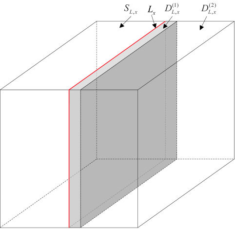
Figure 6: The sources and the partition of destinations with cut $L_{x}$.

Consider a cut plane $L_{x}$ that divides the 3D network into two equal halves, each of which contains $n/2$ nodes, as illustrated in Fig. 6. The set of destinations, $D_{L,x}$, is further partitioned into two groups $D_{L,x}^{(1)}$ and $D_{L,x}^{(2)}$ according to their locations. Here, $D_{L,x}^{(1)}$ denote the sets of destinations located on the cuboid with width one immediately to the right of the cut plane, and $D_{L,x}^{(2)}$ is given by $D_{L,x}\setminus D_{L,x}^{(1)}$. Note that the set $D_{L,x}^{(1)}$ of destinations located very close to the cut plane $L_{x}$ are taken into account separately since, otherwise, their contribution to the aggregate throughput will be excessive, resulting in a loose bound. We start from the following lemma, in which the cut-set bound for erasure networks is characterized assuming no interference, leading to an upper bound on the performance.

Lemma 12 ([31])

For an erasure network divided into two sets $S_{L,x}$ and $D_{L,x}$, the cut-set bound on the aggregate throughput $T_{n}$ is given by

$$T_{n}\leq\sum_{i\in S_{L,x}}\left(1-\prod_{k\in D_{L,x}}\epsilon_{ki}\right),$$ (6)

where $\epsilon_{ki}$ is the erasure probability between source $i\in S_{L,x}$ and destination $k\in D_{L,x}$.

Using the characteristics of random node distribution establishes the following binning lemma.

Lemma 13

Let the 3D network volume be divided into $n$ cubes of unit volume. Then, there are less than $\operatorname{log}n$ nodes inside all cubes whp.

Proof:

This lemma can be proved by slightly modifying the proof of [4, Lemma 1]. ∎

The cut-set upper bound on the aggregate throughput $T_{n}$ is given by

$$T_{n}\leq T_{n}^{(1)}+T_{n}^{(2)},$$

where $T_{n}^{(1)}$ and $T_{n}^{(2)}$ denote the throughputs from the set of sources, $S_{L,x}$, to the sets of corresponding destinations, $D_{L,x}^{(1)}$ and $D_{L,x}^{(2)}$, respectively. The contribution to $T_{n}^{(1)}$ from nodes in $D_{L,x}^{(1)}$ is no greater than one for each node. Since there are no more than $n^{\mu+\nu}\operatorname{log}n$ nodes in $D_{L,x}^{(1)}$ from Lemma 13, the throughput for the set $D_{L,x}^{(1)}$ is upper-bounded by

$$T_{n}^{(1)}=O(n^{\mu+\nu}\operatorname{log}n).$$

Hence, from (6), an upper bound on $T_{n}$ is given by

$$T_{n} \leq a_{0}n^{\mu+\nu}\operatorname{log}n+\sum_{i\in S_{L,x}}\left(1-\prod_{k\in D_{L,x}^{(2)}}\epsilon_{ki}\right)$$

$$\leq a_{0}n^{\mu+\nu}\operatorname{log}n+\sum_{i\in S_{L,x}}\sum_{k\in D_{L,x}^{(2)}}(1-\epsilon_{ki}),$$

where $a_{0}>0$ is some constant independent of $n$. In order to derive an upper bound on $T_{n}^{(2)}$, we would like to consider the network transformation resulting in a regular network with at most $\operatorname{log}n$ nodes in each subcube of unit volume, similarly as in [10, 24]. In this case, we can construct the resulting regular network in which two neighboring nodes are regularly 1 unit of distance apart from each other. Let us divide the left half of the network into $n^{\mu+\nu}$ cuboids of side length $\frac{1}{2}n^{\lambda}\times 1\times 1$. Let $J_{u}$ denote the $u$th cuboid of $S_{L,x}$, i.e., $S_{L,x}=\bigcup_{u=1}^{n^{\mu+\nu}}J_{u}$. Then, $T_{n}^{(2)}$ is bounded by

$$T_{n}^{(2)}\leq\sum_{u=1}^{n^{\mu+\nu}}\sum_{i\in J_{u}}\sum_{k\in D_{L,x}^{(2)}}(1-\epsilon_{ki}).$$ (7)

As depicted in Fig. 7, as we move the nodes that lie in each cube of $J_{m}$ together with the nodes in the cubes of $D_{L,x}^{(2)}$ onto the vertex indicated by the arrows, $T_{n}^{(2)}$ increases since this node displacement leads to a decrement of the Euclidean distance between the associated nodes. Since there are no more than $\operatorname{log}n$ nodes in each unit cube, the modification results in a regular network with at most $\operatorname{log}n$ nodes at each cube vertex on the left and at most $4\operatorname{log}n$ nodes at each cube vertex on the right. Thus, the throughput $T_{n}^{(2)}$ is less than the quantity achieved for a regular network with $\operatorname{log}n$ nodes at each left-hand side vertex and $4\operatorname{log}n$ nodes at each right-hand side vertex. In the following two subsections, we derive upper bounds on the aggregate capacity according to the two path-loss attenuation models.

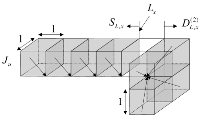
Figure 7: The displacement of the nodes inside the cubes to vertices, indicated by arrows.

V-A Upper Bound Under the Exponential Decay Model

In this subsection, we present a cut-set upper bound on the capacity for the exponential decay model by considering the network transformation to a regular network.

Theorem 3

Suppose a 3D erasure network of size length $n^{\lambda}\times n^{\mu}\times n^{\nu}$ with unit node density under the exponential decay model, where the probability of successful transmission decays exponentially as in (1). Then, the aggregate throughput is upper-bounded by

$$T_{n}=O(n^{\operatornamewithlimits{min}\{1-\lambda,1-\mu,1-\nu\}}(\operatorname{log}n)^{2}).$$

Proof:

We start by assuming a regular network having one node at each unit cube vertex. We first consider the cut plane $L_{x}$. Suppose that the left-hand side nodes are located at positions $(-i_{l}+1,j_{l},k_{l})$ and those on the right-hand side are located at positions $(i_{r},j_{r},k_{r})$. Substituting (1) into (7), $T_{n}^{(2)}$ is bounded by

$$T_{n}^{(2)}$$

$$\leq\sum_{i\in S_{L}}\sum_{k\in D_{L}}\gamma^{d_{ki}}$$

$$\leq\!\!\!\sum_{i_{l}=1,i_{r}=1}^{n^{\lambda}/2}\!\sum_{j_{l}=1,j_{r}=1}^{n^{\mu}}\!\sum_{k_{l}=1,k_{r}=1}^{n^{\nu}}\!\!\!\gamma^{((i_{l}+i_{r}-1)^{2}+(j_{l}-j_{r})^{2}+(k_{l}-k_{r})^{2})^{1/2}}$$

$$=\sum_{i_{r}=1}^{n^{\lambda}/2}\sum_{j_{r}=1}^{n^{\mu}}\sum_{k_{r}=1}^{n^{\nu}}$$

$$~{}~{}~{}\left(\sum_{i_{l}=1}^{n^{\lambda}/2}\sum_{j_{l}=1}^{n^{\mu}}\sum_{k_{l}=1}^{n^{\nu}}\gamma^{((i_{l}+i_{r}-1)^{2}+(j_{l}-j_{r})^{2}+(k_{l}-k_{r})^{2})^{1/2}}\right)$$

$$\leq\sum_{i_{r}=1}^{n^{\lambda}/2}\sum_{j_{r}=1}^{n^{\mu}}\sum_{k_{r}=1}^{n^{\nu}}$$

$$~{}~{}~{}\left(\sum_{v=1}^{\infty}a_{1}(3i_{r}^{2}+6i_{r}v-3i_{r}+3v^{2}-3v+1)\gamma^{i_{r}+v-1}\right)$$

$$\leq\sum_{i_{r}=1}^{n^{\lambda}/2}\sum_{j_{r}=1}^{n^{\mu}}\sum_{k_{r}=1}^{n^{\nu}}\left(\sum_{v=1}^{\infty}a_{1}(3i_{r}^{2}+6i_{r}v+4v^{2})\gamma^{i_{r}+v-1}\right)$$

$$=\sum_{i_{r}=1}^{n^{\lambda}/2}\sum_{j_{r}=1}^{n^{\mu}}\sum_{k_{r}=1}^{n^{\nu}}\left(a_{2}i_{r}^{2}\gamma^{i_{r}}\frac{1}{1-\gamma}+a_{3}i_{r}\gamma^{i_{r}}\frac{1}{(1-\gamma)^{2}}\right.$$

$$~{}~{}~{}\left.+a_{4}\gamma^{i_{r}}\frac{(1+\gamma)}{(1-\gamma)^{3}}\right)$$

$$=\sum_{i_{r}=1}^{n^{\lambda}/2}\sum_{j_{r}=1}^{n^{\mu}}\sum_{k_{r}=1}^{n^{\nu}}\left(a_{5}i_{r}^{2}\gamma^{i_{r}}+a_{6}i_{r}\gamma^{i_{r}}+a_{7}\gamma^{i_{r}}\right)$$

$$=\sum_{i_{r}=1}^{n^{\lambda}/2}n^{\mu+\nu}\left(a_{5}i_{r}^{2}\gamma^{i_{r}}+a_{6}i_{r}\gamma^{i_{r}}+a_{7}\gamma^{i_{r}}\right)$$

$$\leq\sum_{i_{r}=1}^{\infty}n^{\mu+\nu}\left(a_{5}i_{r}^{2}\gamma^{i_{r}}+a_{6}i_{r}\gamma^{i_{r}}+a_{7}\gamma^{i_{r}}\right)$$

$$\leq n^{\mu+\nu}\left(a_{5}\frac{\gamma(1+\gamma)}{(1-\gamma)^{3}}+a_{6}\frac{\gamma}{(1-\gamma)^{2}}+a_{7}\frac{\gamma}{1-\gamma}\right),$$ (8)

where $\{a_{i}\}_{i=1}^{7}$ are positive constants, independent of $n$.

Next, using the fact that our 3D random network is transformed to the regular network with $\operatorname{log}n$ nodes at each left-hand side vertex and $4\operatorname{log}n$ nodes at each right-hand side vertex, $T_{n}^{(2)}$ is finally upper-bounded by

$$T_{n}^{(2)} \leq 4(\operatorname{log}n)^{2}n^{\mu+\nu}$$

$$~{}~{}~{}\cdot\left(a_{5}\frac{\gamma(1+\gamma)}{(1-\gamma)^{3}}+a_{6}\frac{\gamma}{(1-\gamma)^{2}}+a_{7}\frac{\gamma}{1-\gamma}\right),$$

resulting in $T_{n}^{(2)}=O(n^{\mu+\nu}(\operatorname{log}n)^{2})$. Since $T_{n}\leq T_{n}^{(1)}+T_{n}^{(2)}$ and $T_{n}^{(1)}=O(n^{\mu+\nu}\operatorname{log}n)$, it follows that $T_{n}=O(n^{\mu+\nu}(\operatorname{log}n)^{2})$.

If the cuboid is divided into two equal halves by other two cut planes $L_{y}$ and $L_{z}$, then the corresponding upper bounds on the aggregate throughput are given by $T_{n}=O(n^{\lambda+\nu}(\operatorname{log}n)^{2})$ and $T_{n}=O(n^{\lambda+\mu}(\operatorname{log}n)^{2})$, respectively, in a similar fashion. In consequence, by taking the minimum of three upper bound results, it follows that $T_{n}=O(n^{\operatornamewithlimits{min}\{\mu+\nu,\lambda+\nu,\lambda+\mu\}}(\operatorname{log}n)^{2})=O(n^{\operatornamewithlimits{min}\{1-\lambda,1-\mu,1-\nu\}}(\operatorname{log}n)^{2})$, which completes the proof of Theorem 3. ∎

From Theorems 1 and 3, the following discussion is made.

Remark 6

Under the exponential model in the 3D erasure network, the upper bound matches the achievable throughput scaling using the percolation-based 3D highway routing protocol within a polylogarithmic factor. We also remark that, unlike the case of Gaussian network models, the use of the hierarchical cooperation [10] or any sophisticated multiuser detection scheme is not needed to improve the achievable throughput scaling.

V-B Upper Bound Under the Polynomial Decay Model

In this subsection, we present a cut-set upper bound on the capacity for the polynomial decay model. The proof techniques are basically similar to those for the exponential decay model.

Theorem 4

Suppose a 3D erasure network of size length $n^{\lambda}\times n^{\mu}\times n^{\nu}$ with unit node density under the polynomial decay model, where the probability of successful transmission decays polynomially as in (2). Then, when $\alpha>3$, the total throughput $T_{n}$ is upper-bounded by

$$T_{n}=O(n^{\operatornamewithlimits{min}\{1-\lambda,1-\mu,1-\nu\}}(\operatorname{log}n)^{2}).$$

Proof:

Let us first assume a regular network having one node at each unit cube vertex. We start by considering the cut plane $L_{x}$. Suppose that the left-hand side nodes are located at positions $(-i_{l}+1,j_{l},k_{l})$ and those on the right-hand side are located at positions $(i_{r},j_{r},k_{r})$. Substituting (2) into (7), $T_{n}^{(2)}$ is then bounded by

$$T_{n}^{(2)}$$

$$\leq\sum_{i\in S_{L}}\sum_{k\in D_{L}}\frac{1}{d_{ki}^{\alpha}}$$

$$\leq\sum_{i_{l}=1,i_{r}=1}^{n^{\lambda}/2}\sum_{j_{l}=1,j_{r}=1}^{n^{\mu}}$$

$$~{}~{}~{}\sum_{k_{l}=1,k_{r}=1}^{n^{\nu}}\frac{1}{((i_{l}+i_{r}-1)^{2}+(j_{l}-j_{r})^{2}+(k_{l}-k_{r})^{2})^{\alpha/2}}$$

$$\leq\sum_{i_{r}=1}^{n^{\lambda}/2}\sum_{j_{r}=1}^{n^{\mu}}\sum_{k_{r}=1}^{n^{\nu}}$$

$$~{}\left(\!\sum_{i_{l}=1}^{n^{\lambda}/2}\sum_{j_{l}=1}^{n^{\mu}}\sum_{k_{l}=1}^{n^{\nu}}\frac{1}{((i_{l}+i_{r}-1)^{2}+(j_{l}-j_{r})^{2}+(k_{l}-k_{r})^{2})^{\alpha/2}}\!\!\right)$$

$$\leq\sum_{i_{r}=1}^{n^{\lambda}/2}\sum_{j_{r}=1}^{n^{\mu}}\sum_{k_{r}=1}^{n^{\nu}}\left(\sum_{v=1}^{\infty}\frac{a_{1}(3i_{r}^{2}+6i_{r}v-3i_{r}+3v^{2}-3v+1)}{(i_{r}+v-1)^{\alpha}}\right)$$

$$\leq\sum_{i_{r}=1}^{n^{\lambda}/2}\sum_{j_{r}=1}^{n^{\mu}}\sum_{k_{r}=1}^{n^{\nu}}\left(\sum_{v=1}^{\infty}\frac{a_{1}(3i_{r}^{2}+6i_{r}v+4v^{2})}{(i_{r}+v-1)^{\alpha}}\right)$$

$$\mathop{\leq}\limits^{(a)}\sum_{i_{r}=1}^{n^{\lambda}/2}\sum_{j_{r}=1}^{n^{\mu}}\sum_{k_{r}=1}^{n^{\nu}}\left(\sum_{v=1}^{\infty}\frac{a_{1}(3i_{r}^{2}+6i_{r}v+4v^{2})}{i_{r}^{\alpha}v^{\alpha}}\right)$$

$$=\sum_{i_{r}=1}^{n^{\lambda}/2}\sum_{j_{r}=1}^{n^{\mu}}\sum_{k_{r}=1}^{n^{\nu}}$$

$$~{}~{}~{}\left(\frac{3a_{1}}{i_{r}^{\alpha-2}}\sum_{v=1}^{\infty}\frac{1}{v^{\alpha}}+\frac{6a_{1}}{i_{r}^{\alpha-1}}\sum_{v=1}^{\infty}\frac{1}{v^{\alpha-1}}+\frac{4a_{1}}{i_{r}^{\alpha}}\sum_{v=1}^{\infty}\frac{1}{v^{\alpha-2}}\right)$$

$$\leq n^{\mu+\nu}\sum_{i_{r}=1}^{\infty}\left(\frac{a_{2}}{i_{r}^{\alpha-2}}+\frac{a_{3}}{i_{r}^{\alpha-1}}+\frac{a_{4}}{i_{r}^{\alpha}}\right),$$ (9)

where $\{a_{i}\}_{i=1}^{4}$ are positive constants, independent of $n$. Here, (a) follows from the fact that $i_{r}v\leq i_{r}+v-1$.

Next, by using the regular network with $\operatorname{log}n$ nodes at each left-hand side vertex and $4\operatorname{log}n$ nodes at each right-hand side vertex, $T_{n}^{(2)}$ is finally upper-bounded by

$$T_{n}^{(2)} \leq 4(\operatorname{log}n)^{2}n^{\mu+\nu}\sum_{i_{r}=1}^{\infty}\left(\frac{a_{2}}{i_{r}^{\alpha-2}}+\frac{a_{3}}{i_{r}^{\alpha-1}}+\frac{a_{4}}{i_{r}^{\alpha}}\right),$$

thus resulting in $T_{n}^{(2)}=O(n^{\mu+\nu}(\operatorname{log}n)^{2})$ when $\alpha>3$. Since $T_{n}\leq T_{n}^{(1)}+T_{n}^{(2)}$ and $T_{n}^{(1)}=O(n^{\mu+\nu}\operatorname{log}n)$, it follows that $T_{n}=O(n^{\mu+\nu}(\operatorname{log}n)^{2})$ when $\alpha>3$.

If the cuboid is divided into two equal halves by other two cut planes $L_{y}$ and $L_{z}$, then the corresponding upper bounds are given by $T_{n}=O(n^{\lambda+\nu}(\operatorname{log}n)^{2})$ and $T_{n}=O(n^{\lambda+\mu}(\operatorname{log}n)^{2})$, respectively, for $\alpha>3$. Therefore, by taking the minimum of three upper bound results, we have $T_{n}=O(n^{\operatornamewithlimits{min}\{\mu+\nu,\lambda+\nu,\lambda+\mu\}}(\operatorname{log}n)^{2})=O(n^{\operatornamewithlimits{min}\{1-\lambda,1-\mu,1-\nu\}}(\operatorname{log}n)^{2})$ for $\alpha>3$, which completes the proof of Theorem 4. ∎

By comparing the results in Theorems 1–4, we have the following observations.

Remark 7

It turns out that the upper bounds for both erasure channel models are of the same order. Moreover, it is shown that the upper bound for the polynomial decay model also matches the corresponding achievable throughput scaling within a polylogarithmic factor when $\alpha>3$; that is, the routing protocol based on the percolation theory is order-optimal for all operating regimes under the exponential decay model and for $\alpha>3$ under the polynomial decay model.

VI Extension to the Dense Network Scenario

So far, we have considered extended networks, where the density of nodes is fixed and the network volume scales as $n$. In this section, as another network configuration, we consider a dense erasure network, where $n$ nodes are uniformly and independently distributed in a cuboid of unit volume, and show its capacity scaling laws.

First, we would like to address the Gaussian channel setup. In extended 3D Gaussian networks, the Euclidean distance between nodes is increased by a factor of $n^{1/3}$, compared to the dense network case, and hence for the same transmit powers, the received powers are all decreased by a certain factor. Equivalently, by re-scaling space, an extended Gaussian network can be regarded as a dense Gaussian network with the average per-node power constraint reduced to a certain factor instead of full power while the received signal-to-interference-and-noise ratios are maintained as $\Omega(1)$ (refer to [10, Section V] for more details).

In the light of the above observation made in Gaussian networks, in the dense erasure network, the channel models in (1) and (2) need to be changed in such a way that the distance $d_{ki}$ between nodes $i$ and $k$ is scaled up to $d_{ki}n^{1/3}$, which results in the same erasure events at the receiver (i.e., the same received signal power) for both network configurations. More precisely, in the dense erasure network, we use the following erasure probabilities $\epsilon_{ki}=1-\gamma^{d_{ki}n^{1/3}}$ and $\epsilon_{ki}=1-\frac{1}{(d_{ki}n^{1/3})^{\alpha}}$ for the exponential and polynomial decay models, respectively.

Now, let us show the achievability result in the dense network. It is obvious to see that the achievable transmission rates $R(d)$ within distance $d$ are the same as Lemmas 4 and 8 since the number of required time slots in the $t$-TDMA scheme has still the same order. Therefore, the achievable throughput scaling laws for the dense network are the same as those for the extended network shown in Theorems 1 and 2. Let us turn to showing the upper bound results in the dense network. Since the distance between nodes is re-scaled by $\frac{1}{n^{1/3}}$, we can similarly use the bounding technique as in (8) and (9). Thus, the upper bounds for both exponential and polynomial decay models are the same as Theorems 3 and 4, respectively. In consequence, the capacity scaling laws for the extended erasure network still hold for the dense erasure network.

VII Concluding Remarks

The capacity scaling was completely characterized for a general 3D erasure random network using two fundamental path-loss attenuation models, i.e., the polynomial and exponential decay models for the erasure probability. For the two erasure models, achievable throughput scaling laws were derived by introducing the 3D percolation highway system, where packets are delivered through the highways in $x$, $y$, and $z$ directions. Our result indicated that the achievable throughput scaling in 3D space is much greater than that in 2D space since more geographic diversity can be exploited in 3D space. Cut-set upper bounds were also analyzed along with the network transformation argument. It turned out that the upper bounds match the achievable throughput scaling laws within a polylogarithmic factor for all operating regimes under the exponential decay model and for $\alpha>3$ under the polynomial decay model. Further investigation of the capacity scaling law for 3D erasure networks in the presence of node mobility remains for future work. Suggestions for further research also include characterizing the capacity scaling when $\alpha\leq 3$ under the polynomial decay model.

Appendix A Proof of Lemma 1

The proof of this lemma essentially follows that of [4, Theorem 5] with a slight modification. Since the event of having a left-to-right crossing of $R_{xz,x}^{j}$ is an increasing event (see [4, Appendix I] for the explanation of the increasing event), for all $0<p^{\prime}<p<1$, we have

$$1-\Pr\{C_{xz,x}^{j}>\delta\operatorname{log}m_{z}\} \leq\left(\frac{p}{p-p^{\prime}}\right)^{\delta\operatorname{log}m_{z}}$$

$$~{}~{}~{}\times(1-P_{p^{\prime}}(R_{xz,x}^{j\leftrightarrow})),$$

where $R_{xz,x}^{j\leftrightarrow}$ is the event that there exists a left-to-right crossing of rectangle $R_{xz,x}^{j}$ and $P_{p}(R_{xz,x}^{j\leftrightarrow})$ is the probability that the event $R_{xz,x}^{j\leftrightarrow}$ occurs when the probability of an open edge is given by $p$. For $p>\frac{2}{3}$, we have

$$P_{p}(R_{xz,x}^{i\leftrightarrow}) \geq 1-\frac{4}{3}(m_{x}+1)e^{-(\kappa\operatorname{log}m_{z}-\epsilon_{m})(-\operatorname{log}(3(1-p))))}$$

$$\geq 1-\frac{4}{3}(m_{x}+1)m_{z}^{\kappa\operatorname{log}(3(1-p))}(3(1-p))^{-\epsilon_{m}},$$

where the first inequality follows from the same argument as in the proof of [4, Proposition 2]. By letting $p^{\prime}=2p-1$, it is seen that $p^{\prime}>\frac{2}{3}$ due to $p>\frac{5}{6}$. From [4, Lemma 6], we thus have

$$\Pr\{C_{xz,x}^{i}\leq\delta\operatorname{log}m_{z}\}$$

$$\leq\left(\frac{p}{p-p^{\prime}}\right)^{\delta\operatorname{log}m_{z}}\frac{4}{3}(m_{x}+1)m_{z}^{\kappa\operatorname{log}(3(1-p^{\prime}))}(3(1-p^{\prime}))^{-\epsilon_{m}}$$

$$\leq\frac{4}{3}(m_{x}+1)m_{z}^{\delta\operatorname{log}\frac{p}{1-p}+\kappa\operatorname{log}(6(1-p))}(6(1-p))^{-\epsilon_{m}}.$$

The probability of having at most $\delta\operatorname{log}m_{z}$ edge-disjoint left-to-right crossings in every rectangle $R_{xz,x}^{i}$ is given by

$$\Pr\{N_{xz,x}\leq\delta\operatorname{log}m_{z}\}$$

$$=\left(\Pr\{C_{xz,x}^{i}\leq\delta\operatorname{log}m_{z}\}\right)^{\frac{m_{z}}{\kappa\operatorname{log}m_{z}-\epsilon_{m}}}$$

$$\leq\left(\frac{4}{3}(m_{x}+1)m_{z}^{\delta\operatorname{log}\frac{p}{1-p}+\kappa\operatorname{log}(6(1-p))}\right.$$

$$~{}~{}~{}\left.\times(6(1-p))^{-\epsilon_{m}}\right)^{\frac{m_{z}}{\kappa\operatorname{log}m_{z}-\epsilon_{m}}}$$

$$=\left(\frac{4}{3}((m_{z})^{\lambda/\nu}\frac{1}{c^{\nu/\lambda}}+1)m_{z}^{\delta\operatorname{log}\frac{p}{1-p}+\kappa\operatorname{log}(6(1-p))}\right.$$

$$~{}~{}~{}\left.\times(6(1-p))^{-\epsilon_{m}}\right)^{\frac{m_{z}}{\kappa\operatorname{log}m_{z}-\epsilon_{m}}}.$$ (A.1)

The right-hand side of (A) tends to zero if

$$\frac{\lambda}{\nu}+\delta\operatorname{log}\frac{p}{1-p}+\kappa\operatorname{log}(6(1-p))<-1$$ (A.2)

since $\lim_{x\rightarrow\infty}\left(\frac{1}{x}\right)^{x}=0$. If the following inequality is fulfilled, then we can choose sufficiently small $\delta$ such that (A.2) is satisfied:

$$1+\frac{\lambda}{\nu}+\kappa\operatorname{log}(6(1-p))<0.$$

In a similar way, if $1+\frac{\nu}{\lambda}+\kappa\operatorname{log}(6(1-p))<0$, then one can show that $\Pr\{N_{xz,z}\leq\delta\operatorname{log}m_{x}\}\rightarrow 0$ by choosing $\delta$ small enough to satisfy $\frac{\nu}{\lambda}+\delta\operatorname{log}\frac{p}{1-p}+\kappa\operatorname{log}(6(1-p))<-1$. This completes the proof of this lemma.

References

- [1] A. Lo, Y. W. Law, and M. Jacobsson, “A cellular-centric service architecture for machine-to-machine (M2M) communications,” IEEE Wireless Commun., vol. 20, no. 5, pp. 143–151, Oct. 2013.
- [2] P. Gupta and P. R. Kumar, “The capacity of wireless networks,” IEEE Trans. Inform. Theory, vol. 46, no. 2, pp. 388–404, Mar. 2000.
- [3] D. E. Knuth, “Big omicron and big omega and big theta,” ACM SIGACT News, vol. 8, no. 2, pp. 18–24, Apr.-Jun. 1976.
- [4] M. Franceschetti, O. Dousse, D. N. C. Tse, and P. Thiran, “Closing the gap in the capacity of wireless networks via percolation theory,” IEEE Trans. Inform. Theory, vol. 53, no. 3, pp. 1009–1018, Mar. 2007.
- [5] P. Gupta and P. R. Kumar, “Towards an information theory of large networks: an achievable rate region,” IEEE Trans. Inform. Theory, vol. 49, no. 8, pp. 1877–1894, Aug. 2003.
- [6] W.-Y. Shin, S.-Y. Chung, and Y. H. Lee, “Parallel opportunistic routing in wireless networks,” IEEE Trans. Inform. Theory, vol. 59, no. 10, pp. 6290–6300, Oct. 2013.
- [7] Y. Nebat, R. L. Cruz, and S. Bhardwaj, “The capacity of wireless networks in nonergodic random fading,” IEEE Trans. Inform. Theory, vol. 55, no. 6, pp. 2478–2493, June 2009.
- [8] A. El Gamal, J. Mammen, B. Prabhakar, and D. Shah, “Optimal throughput-delay scaling in wireless networks–Part I: The fluid model,” IEEE Trans. Inform. Theory, vol. 52, no. 6, pp. 2568–2592, June 2006.
- [9] M. J. Neely and E. Modiano, “Capacity and delay tradeoffs for ad hoc mobile networks,” IEEE Trans. Inform. Theory, vol. 51, no. 6, pp. 1917–1937, June 2005.
- [10] A. Özgür, O. Lévêque, and D. N. C. Tse, “Hierarchical cooperation achieves optimal capacity scaling in ad hoc networks,” IEEE Trans. Inform. Theory, vol. 53, no. 10, pp. 3549–3572, Oct. 2007.
- [11] J. Ghaderi, L.-L. Xie, and X. Shen, “Hierarchical cooperation in ad hoc networks: Optimal clustering and achievable throughput,” IEEE Trans. Inform. Theory, vol. 55, no. 8, pp. 3425–3436, Aug. 2009.
- [12] U. Niesen, P. Gupta, and D. Shah, “On capacity scaling in arbitrary wireless networks,” IEEE Trans. Inform. Theory, vol. 55, no. 9, pp. 3959–3982, Sept. 2009.
- [13] M. Grossglauser and D. N. C. Tse, “Mobility increases the capacity of ad hoc wireless networks,” IEEE/ACM Trans. Networking, vol. 10, no. 4, pp. 477–486, Aug. 2002.
- [14] V. R. Cadambe and S. A. Jafar, “Interference alignment and degrees of freedom of the -user interference channel,” IEEE Trans. Inform. Theory, vol. 54, no. 8, pp. 3425–3441, Aug. 2008.
- [15] G. Zhang, Y. Xu, X. Wang, and M. Guizani, “Capacity of hybrid wireless networks with directional antenna and delay constraint,” IEEE Trans. Commun., vol. 58, no. 7, pp. 2097–2106, July 2010.
- [16] P. Li, C. Zhang, and Y. Fang, “The capacity of wireless ad hoc networks using directional antennas,” IEEE Trans. Mobile Comput., vol. 10, no. 10, pp. 1374–1387, Oct. 2011.
- [17] J. Yoon, W.-Y. Shin, and S.-W. Jeon, “Elastic routing in wireless networks with directional antennas,” in Proc. IEEE Int. Symp. Inf. Theory (ISIT), Honolulu, HI, Jun./Jul. 2014, pp. 1001–1005.
- [18] O. Dousse, P. Thiran, and M. Hasler, “Connectivity in ad-hoc and hybrid networks,” in Proc. IEEE INFOCOM, New York, NY, June 2002, pp. 1079–1088.
- [19] S. R. Kulkarni and P. Viswanath, “Throughput scaling for heterogeneous networks,” in Proc. IEEE Int. Symp. Inf. Theory (ISIT), Yokohama, Japan, Jun./Jul. 2003, p. 452.
- [20] U. C. Kozat and L. Tassiulas, “Throughput capacity of random ad hoc networks with infrastructure support,” in Proc. ACM MobiCom, San Diego, CA, Sept. 2003, pp. 55–65.
- [21] B. Liu, Z. Liu, and D. Towsley, “On the capacity of hybrid wireless networks,” in Proc. IEEE INFOCOM, San Francisco, CA, Mar./Apr. 2003, pp. 1543–1552.
- [22] A. Zemlianov and G. de Veciana, “Capacity of ad hoc wireless networks with infrastructure support,” IEEE J. Select. Areas Commun., vol. 23, no. 3, pp. 657–667, Mar. 2005.
- [23] B. Liu, P. Thiran, and D. Towsley, “Capacity of a wireless ad hoc network with infrastructure,” in Proc. ACM MobiHoc, Montréal, Canada, Sept. 2007, pp. 239–246.
- [24] W.-Y. Shin, S.-W. Jeon, N. Devroye, M. H. Vu, S.-Y. Chung, Y. H. Lee, and V. Tarokh, “Improved capacity scaling in wireless networks with infrastructure,” IEEE Trans. Inform. Theory, vol. 57, no. 8, pp. 5088–5102, Aug. 2011.
- [25] M. Doddavenkatappa, M. C. Chan, and A. L. Ananda, “Indriya: A low-cost, 3d wireless sensor network testbed,” in Lecture Notes of the Institute for Computer Sciences, Social-Informatics and Telecommunications Engineering.
- [26] M.-S. Lin, J.-S. Leu, K.-H. Li, and J.-L. C. Wu, “Zigbee-based Internet of Things in 3D terrains,” Computers & Electrical Engineering, vol. 39, no. 6, pp. 1667–1683, Aug. 2013.
- [27] P. Gupta and P. Kumar, “Internets in the sky: The capacity of three dimensional wireless networks,” Commun. Inf. Syst., vol. 1, pp. 33–50, 2001.
- [28] P. Li, M. Pan, and Y. Fang, “Capacity bounds of three-dimensional wireless ad hoc networks,” IEEE/ACM Trans. Netw., vol. 20, no. 4, pp. 1304–1315, Aug. 2012.
- [29] M. Franceschetti, M. D. Migliore, and P. Minero, “The capacity of wireless networks: information-theoretic and physical limits,” IEEE Trans. Inform. Theory, vol. 55, no. 8, pp. 3413–3424, Aug. 2009.
- [30] C. Hu, X. Wang, Z. Yang, J. Zhang, Y. Xu, and X. Gao, “A geometry study on the capacity of wireless networks via percolation,” IEEE Trans. Commun., vol. 58, no. 10, pp. 2916–2925, Oct. 2010.
- [31] A. Dana, R. Gowaikar, and B. Hassibi, “Capacity of wireless erasure networks,” IEEE Trans. Inform. Theory, vol. 32, no. 3, pp. 789–804, Mar. 2006.
- [32] J. W. Lee, R. L. Urbanke, and R. E. Blahut, “Turbo codes in binary erasure channel,” IEEE Trans. Inf. Theory, vol. 54, no. 4, pp. 1765–1773, Apr. 2008.
- [33] R. G. Jabar and J. G. Andrews, “A lower bound on the capacity of wireless erasure networks,” IEEE Trans. Inf. Theory, vol. 57, no. 10, pp. 6502–6513, Oct. 2011.
- [34] A. Tulino, S. Verdú, G. Caire, and S. Shamai, “The Gaussian erasure channel,” in Proc. Int. Symp. Inf. Theory (ISIT), Nice, France, June/July 2007, pp. 1721–1725.
- [35] S. Verdú and T. Weissman, “The information lost in erasures,” IEEE Trans. Inform. Theory, vol. 54, no. 11, pp. 5030–5058, Nov. 2008.
- [36] B. Smith, P. Gupta, and S. Vishwanath, “Routing is order-optimal in broadcast erasure networks with interference,” in Proc. IEEE Int. Symp. Inf. Theory (ISIT), Nice, France, June 2007, pp. 141–145.
- [37] W.-Y. Shin and A. Kim, “Capacity scaling of infrastructure-supported erasure networks,” IEEE Commun. Lett., vol. 15, no. 5, pp. 485–487, May 2011.
- [38] B. Smith and S. Vishwanath, “Asymptotic transport capacity of wireless erasure networks,” in Proc. 44th Allerton Conf. on Commun., Control, and Computing, Monticello, Illinois, 2006, pp. 27–29.
- [39] B. Smith, P. Gupta, and S. Vishwanath, “Routing versus network coding in erasure networks with broadcast and interference constraints,” in Proc. IEEE Military Commun. Conf. (MILCOM), Orlando, FL, Oct. 2007, pp. 1–5.
- [40] C. Jeong and W.-Y. Shin, “Capacity scaling of hybrid erasure networks based on polynomial power-law,” IEEE Commun. Lett., vol. 17, no. 5, pp. 1024–1027, May 2013.
- [41] B. M. Smith, Capacities of Erasure Networks. US: ProQuest, 2008.
- [42] T. M. Cover and J. A. Thomas, Elements of Information Theory. New York: Wiley, 1991.