DESY 16-061, KA-TP-14-2016, TTK-16-14 SusHi Bento: Beyond NNLO and the heavy-top limit

Abstract

Version 1.6.0 of the code SusHi is presented. Concerning inclusive CP-even Higgs production in gluon fusion, the following new features with respect to previous versions have been implemented: expansion of the partonic cross section in the soft limit, i.e. around $x=M_{\text{H}}^{2}/\hat{s}\to 1$; N³LO QCD corrections in terms of the soft expansion; top-quark mass suppressed terms through NNLO; matching to the cross section at $x\to 0$ through N³LO. For CP-even and -odd scalars, an efficient evaluation of the renormalization-scale dependence is included, and effects of dimension-5 operators can be studied, which we demonstrate for the SM Higgs boson and for a CP-even scalar with a mass of $750$ GeV. In addition, as a generalization of the previously available $b\bar{b}\to H$ cross section, SusHi_1.6.0 provides the cross section for charged and neutral Higgs production in the annihilation of arbitrary heavy quarks. At fixed order in perturbation theory, SusHi thus allows to obtain Higgs cross-section predictions in different models to the highest precision known today. For the SM Higgs boson of $M_{\text{H}}=125$ GeV, SusHi yields $48.28$ pb for the gluon-fusion cross section at the LHC at $13$ TeV. Simultaneously, SusHi provides the renormalization-scale uncertainty of $\pm 1.97$ pb.

PROGRAM SUMMARY
Program title: SusHi.
Licensing provisions: GNU General Public License 3 (GPL).
Programming language: Fortran 77.
Reference of previous version:
http://dx.doi.org/10.1016/j.cpc.2013.02.006 .
Does the new version supersede the previous version?: Yes. The new version also includes all features of previous versions.
Reasons for the new version:
Compared to version 1.0.0 the newest SusHi version 1.6.0 now supports the 2-Higgs-Doublet-Model (2HDM) and the next-to-minimal supersymmetric standard model (NMSSM). The effects of dimension-5 operators in the calculation of the gluon-fusion cross section can be studied. It allows to calculate the Higgs production cross section from the annihilation of heavy quarks and includes various new features which improve the gluon-fusion cross-section prediction and the associated uncertainty estimate. Links to external codes 2HDMC, MoRe-SusHi and MadGraph5_aMC@NLO can be established.
Summary of revisions:
Inclusion of 2HDM, NMSSM; Improvements in the prediction of the gluon-fusion cross section: Top-quark mass terms up to next-to-next-to leading order, soft expansion and next-to-next-to-next-to leading order corrections in the heavy top-quark effective theory, top squark corrections up to next-to-next-to leading order; dimension-5 operators; analytic determination of the renormalization scale dependence. Inclusion of heavy-quark annihilation cross sections. Link to MoRe-SusHi for the calculation of resummed transverse-momentum distributions.
Nature of problem:
Calculation of inclusive and exclusive Higgs production cross sections in gluon fusion and heavy-quark annihilation in the SM and extended Higgs sectors through next-to-leading order QCD, including (next-to-)next-to-next-to-leading order top-(s)quark contributions and electroweak effects.
Solution method: Numerical Monte Carlo integration.
References: http://sushi.hepforge.org

1 Introduction

Since the year 2012, an important task of particle physics is to fully measure the properties of the Higgs boson with mass $M_{\text{H}}\approx 125$ GeV discovered at the Large Hadron Collider (LHC) [1, 2]. At the same time, the search for additional Higgs bosons, which are predicted in many extended theories, is among the main missions of the LHC experiments. For this purpose, the knowledge of the corresponding production cross sections with high precision is of great relevance. The latest efforts in this direction are regularly summarized in the reports of the “LHC Higgs cross section working group”[3, 4, 5, 6].

In this paper, we describe the new features that have been implemented in version 1.6.0 of the program SusHi [7, 8]. SusHi is a Fortran code which calculates Higgs-boson production cross sections through gluon fusion and bottom-quark annihilation in the Standard Model (SM), general Two-Higgs-Doublet Models (2HDM), the Minimal Supersymmetric Standard Model (MSSM) as well as its next-to-minimal extension (NMSSM), see Ref. [9]. Some of these additions to SusHi directly improve the theoretical predictions of the cross section; others are provided to allow for more sophisticated uncertainty estimates of these predictions. The new features are the following:

• SusHi now includes the next-to-next-to-next-to-leading order (N³LO) terms for the gluon-fusion cross section of a CP-even Higgs boson in the heavy-top limit as described in Refs. [19, 20, 21, 22].

• It provides the so-called soft expansion of the gluon-fusion cross section around the threshold of Higgs-boson production at $x\equiv M_{\phi}^{2}/\hat{s}=1$, where $\hat{s}$ denotes the partonic center-of-mass energy and $M_{\phi}$ the Higgs-boson mass. This expansion is available for the cross sections in the heavy-top limit up to N³LO for CP-even Higgs bosons. At next-to-leading order (NLO) and next-to-NLO (NNLO), the exact $x$-dependence is still available, of course, and remains the default.

• In addition, SusHi_1.6.0 includes top-quark mass effects to the gluon-fusion cross section of a CP-even Higgs boson in the heavy-top limit up to NNLO, implemented through an expansion in inverse powers of the top-quark mass as described in Refs. [23, 24, 25, 26, 27, 28, 29]. The exact top-mass dependence at lowest order can be factored out. We remark that this feature is most interesting at NNLO, of course, since at leading order (LO) and NLO, SusHi also provides the full quark-mass dependence.

• A matching of the soft expansion to the high-energy limit [23, 24, 25], i.e. $x\to 0$, is available through N³LO.

• The renormalization-scale dependence of the gluon-fusion cross section within an arbitrary interval is calculated in a single SusHi run.

• The effect of dimension-5 operators to the gluon-fusion cross section can be taken into account through N³LO QCD for the inclusive cross section, and at LO and NLO (i.e. $\alpha_{s}^{3}$) for the Higgs transverse momentum ($p_{T}$) distribution and (pseudo)rapidity distribution, respectively.

• Higgs-boson production cross sections through heavy-quark annihilation are implemented along the lines of Ref. [30], both for the NNLO QCD inclusive cross section, as well as for more exclusive cross sections up to NLO QCD.

All of the described features are applicable to Higgs-boson production in the theoretical models currently implemented in SusHi, even though some only work for low Higgs masses below the top-quark threshold $M_{\phi}<2M_{\text{t}}$ or for CP-even Higgs bosons.

Our paper is organized as follows: We start with a brief general overview of the code SusHi in Section 2, and subsequently present the new features implemented for the prediction of the gluon-fusion cross section in Section 3. This includes a theoretical description of the soft expansion, the inclusion of N³LO terms and the top-quark mass effects in Sections 3.1–3.3. We proceed with a description of the “RGE procedure” to determine the renormalization-scale dependence of the gluon-fusion cross section in Section 3.4, and finally describe the implementation of an effective Lagrangian including dimension-5 operators in Section 3.5. The implementation of heavy-quark annihilation cross sections is described in Section 4. Numerical results are presented in Section 5; they also include a comparison of our results with the most recent literature. In A we present a collection of example input blocks of SusHi, which contain example settings for the various input entries introduced in previous and the newest release.

2 The program SusHi

SusHi is a program originally designed to describe Higgs production in gluon fusion and bottom-quark annihilation in the MSSM. It collects a number of results from the literature valid through N³LO in the strong coupling constant, and combines them in a consistent way. We subsequently discuss the present theoretical knowledge of the calculation of the gluon fusion and bottom-quark annihilation cross sections and their inclusion in SusHi.

It is well-known that QCD corrections to the gluon-fusion process $gg\rightarrow\phi$ [31], mediated through heavy quarks in the SM, are very large. NLO QCD corrections are known for general quark masses [32, 33, 34, 35, 36, 37]. In the heavy-top limit, an effective theory can be constructed by integrating out the top quark. In this case, NNLO corrections have been calculated a long time ago [38, 39, 40]. The N³LO contributions were only recently obtained in Refs. [41, 42, 19, 20, 22], while various parts of the N³LO calculation have been calculated independently [43, 44, 45, 46, 47, 48, 49, 50, 21, 51, 52, 53, 54, 55, 56]. Approximate N³LO results were presented in Refs. [16, 17, 57]. Effects of a finite top-quark mass at NNLO were approximately taken into account in Refs. [24, 25, 26, 27, 28, 29, 23].

Many of these effects can be taken into account in the latest version of SusHi; this will be discussed in detail in Section 3. Electroweak corrections [58, 59, 60] can be included as well, either in terms of the full SM electroweak correction factor, or restricted to the corrections mediated by light quarks, the latter being a more conservative estimate in certain BSM scenarios. For completeness, we note that effects beyond fixed order have been addressed through soft-gluon resummation [61, 62, 63, 64, 65, 66, 67, 18], but those are not included in SusHi.

If requested in the input file, SusHi uses the SM results described above also for the 2HDM, the MSSM or the NMSSM through the proper rescaling of the Yukawa couplings. In supersymmetric models, also squarks induce an interaction of the Higgs boson to two gluons. In the MSSM, the corresponding NLO virtual contributions, involving squarks, quarks and gluinos, are either known in an expansion of inverse powers of heavy SUSY masses [68, 69, 70] or in the limit of a vanishing Higgs mass, see Refs. [71, 72, 73, 74]. In this limit, even NNLO corrections of stop-induced contributions are known, see Refs. [75, 76]; an approximation of these effects [77] is included in SusHi, see Ref. [78]. Whereas for the MSSM SusHi relies on both expansions, for the NMSSM the NLO virtual corrections are purely based on an expansion in heavy SUSY masses [9]. We note that numerical results for the exact NLO virtual contributions involving squarks, quarks, and gluinos were presented in Refs. [79, 80], and analytic results for the pure squark-induced contributions can be found in Refs. [36, 37, 81].

The associated production of a Higgs boson with bottom quarks, $pp\rightarrow b\bar{b}\phi$, is of particular relevance for Higgs bosons, where the Yukawa coupling to bottom quarks is enhanced. This happens in models with two Higgs doublets, for example, if $\tan\beta$, the ratio of the vacuum expectation values of the two neutral Higgs fields, is large. SusHi includes the cross section for this process in the so-called 5-flavor scheme, i.e. for the annihilation process $b\bar{b}\to\phi$. The inclusive cross section for this process is implemented at NNLO QCD [82, 83]; it is reweighted by effective Yukawa couplings in the model under consideration. SusHi_1.6.0 now also includes general heavy-quark annihilation cross sections [30] at NNLO QCD, which we will describe in Section 4.

For completeness we note that SusHi can be linked to FeynHiggs [84, 85, 86, 87] and 2HDMC [88] to obtain consistent sets of parameters in the MSSM or the 2HDM, respectively.

SusHi is controlled via an SLHA-style [89] input file. In the following, we will refer to the entries of a Block "NAME" and their possible values as NAME(ENTRY)=VALUE. If more than one value is required, we write NAME(ENTRY)={VALUE1,VALUE2,$\dots$} or, when referring only to one specific value, NAME(ENTRY,1)=VALUE1, etc. In A we include input blocks with example settings for the various new input entries.

3 Higgs production through gluon fusion

The hadronic cross section for Higgs production in gluon fusion can be written as

$$\begin{split}\sigma(pp\to H+X)=\sum_{i,j\in\{q,\bar{q},g\}}\tilde{\phi}_{i}\otimes\tilde{\phi}_{j}\otimes\hat{\sigma}_{ij}\,,\end{split}$$ (1)

where $\phi_{i}(x,\mu_{\text{F}})=\tilde{\phi}_{i}(x,\mu_{\text{F}})/x$ are parton densities, $q$ ($\bar{q}$) denotes the set of all (anti-)quarks ($q=t$ and $\bar{q}=\bar{t}$ can be neglected), and $\otimes$ is the convolution defined as

$$\begin{split}(f\otimes g)(z)\equiv\int_{0}^{1}{\rm d}x_{1}\int_{0}^{1}{\rm d}x_{2}f(x_{1})g(x_{2})\delta(z-x_{1}x_{2})\,.\end{split}$$ (2)

The perturbative expansion of the partonic cross section,

$$\begin{split}\hat{\sigma}_{ij,\text{{N${}^{n}$LO}}}&=\sum_{l=0}^{n}\hat{\sigma}^{(l)}_{ij}\,,\end{split}$$ (3)

can be represented in terms of Feynman diagrams where the external partons couple to the Higgs bosons through a top-, bottom-, or charm-quark loop (contributions from lighter quarks are negligible).

The first two terms in the perturbative expansion of $\hat{\sigma}_{ij}$ ($l=0,1$ in Eq. (3)) are known for general quark mass and included in SusHi_1.6.0. For the top-quark contribution, the NNLO term $\hat{\sigma}^{(2)}_{ij}$ has been evaluated on the basis of an effective Higgs-gluon interaction vertex which results from integrating out the top quark from the SM Lagrangian. At NLO, it has been checked that this results in an excellent approximation of the NLO QCD correction factor to the LO cross section, even for rather large Higgs-boson masses. At NNLO, the validity of the heavy-top limit for the QCD corrections factor was investigated through the calculation of a number of terms in an expansion around $M_{\text{t}}^{2}\gg\hat{s},M_{\phi}^{2}$, and matching it to the high-energy limit of $\hat{\sigma}^{(2)}_{ij}$ [24, 25, 26, 27, 28, 29, 23]. It was found that the mass effects to the QCD correction factor are at the sub-percent level.

Recently, also the N³LO-term $\hat{\sigma}_{ij}^{(3)}$ has become available in terms of a soft expansion and assuming the heavy-top limit. We will comment on its implementation in the latest release of SusHi in Section 3.2.

The exact NLO and the approximate higher order results for the cross section are combined in SusHi through the formula

$$\begin{split}\sigma_{\text{{X}}}&=\sigma_{\text{{NLO}}}+\Delta_{\text{{X}}}\sigma^{t}\,,\qquad\Delta_{\text{{X}}}\sigma^{t}\equiv(1+\delta_{\text{EW}})\sigma^{t}_{\text{{X}}}-\sigma_{\text{{NLO}}}^{t}\,,\end{split}$$ (4)

where $\sigma_{\text{{NLO}}}$ refers to the NLO cross section with exact top-, bottom- and charm-mass dependence, while $\sigma^{t}_{\text{{X}}}$ (X$=$NⁿLO, $n\geq 1$) is obtained in the limit of a large top-quark mass. Electroweak effects [58], encoded in $\delta_{\text{EW}}$, are included by assuming their full factorization from the QCD effects, as suggested by Ref. [90] for a SM Higgs boson. In BSM scenarios, this assumption may be no longer justified. SusHi therefore provides an alternative way to include electroweak effects which is based solely on the light-quark contributions to the electroweak correction factor; for details, we refer the reader to Refs. [78, 7]. For our purpose, it suffices to assume Eq. (4). The new release of SusHi provides various approximations to evaluate $\sigma^{t}_{\text{{X}}}$, in particular through expansions in $1/M_{\text{t}}$, and expansions around $\hat{s}=M_{\phi}^{2}$.

In addition to $\sigma_{\text{{X}}}$, which can be found in Block SUSHIggh, SusHi also outputs the individual terms of Eq. (4). The exact LO and NLO cross sections are collected in Block XSGGH, while the $\sigma^{t}_{\text{{X}}}$ are given in Block XSGGHEFF, which also contains the electroweak correction term $\delta_{\text{EW}}$, if requested.

It is understood that the NⁿLO terms in Eq. (4) are evaluated with NⁿLO PDFs. Note that this means that, for example, $\Delta_{\text{{NNLO}}}\sigma^{t}$ is not simply the convolution of $\hat{\sigma}^{t,(2)}$ with NNLO PDFs, but retains a sensitivity to $\hat{\sigma}^{t,(1)}$. Thus, the final result for the NNLO gluon-fusion cross section obtained from SusHi through Eq. (4) depends on the approximation applied to the evaluation of both $\hat{\sigma}^{t,(2)}$ and $\hat{\sigma}^{t,(1)}$. If electroweak effects are included, this even holds for SusHi’s final result for $\sigma_{\text{{NLO}}}$ due to the definition of $\Delta_{\text{X}}\sigma^{t}$ in Eq. (4).

In the remainder of this section, we first discuss the soft expansion around the threshold of Higgs production, $\hat{s}=M_{\phi}^{2}$, in Section 3.1. The implementation of N³LO contributions is described in Section 3.2, and top-quark mass effects through NNLO as well as the matching to the high-energy limit in Section 3.3. While these features are only available for CP-even Higgs bosons (partially in a certain range of Higgs-boson masses $M_{\phi}$ only), the analytic calculation of the $\mu_{\text{R}}$ dependence of the gluon-fusion cross section described in Section 3.4 is available for all Higgs bosons. The inclusion of dimension-5 operators is discussed in Section 3.5.

3.1 Soft expansion

The NLO and NNLO coefficients of $\sigma^{t}$ are approximated very well by the first few terms in an expansion around the “soft limit”, $x\to 1$. In fact, the gain of the full $\hat{s}$-dependence becomes doubtful anyway when working in the heavy-top limit, since the latter formally breaks down for $\hat{s}>4M_{\text{t}}^{2}$, meaning $x\lesssim 0.13$ for $M_{\text{H}}=125$ GeV. Apart from the exact $\hat{s}$-dependence at LO, NLO, and NNLO, SusHi_1.6.0 provides the soft expansion of the cross section for CP-even Higgs production through order $(1-x)^{16}$ at these perturbative orders, and also at N³LO (for more details on the latter, see Section 3.2).

The precise way in which the soft expansion is applied is governed by the new Block GGHSOFT. Each line in this block contains four integers:

⬇

Block GGHSOFT

<entry> <n1> <n2> <n3>

Following Section 2, we will refer to such a line as GGHSOFT(<entry>)={<n1>,<n2>,<n3>} in the text, and to the individual entries as GGHSOFT(<entry>,1)=<n1>, etc. The integer GGHSOFT($n$,1) determines whether the soft expansion is applied (=1) or not (=0) at order NⁿLO. Setting GGHSOFT($n$)={1,$N,a$} evaluates the soft expansion of $\hat{\sigma}^{t,(n)}_{ij}$ in the following way:

$$\begin{split}\hat{\sigma}^{t}_{ij}\to\hat{\sigma}^{t}_{ij,N}\equiv x^{a}{\cal T}^{x}_{N}\left(\frac{\Delta\hat{\sigma}^{t}_{ij}}{x^{a}}\right)\,,\end{split}$$ (5)

where ${\cal T}^{x}_{N}$ denotes the asymptotic expansion around $x=1$ through order $(1-x)^{N}$, and $a$ is a non-negative integer. Setting GGHSOFT($n$,2)=-1 will keep only the soft and collinear terms, whose $x$ dependence is given by

$$\begin{split}\delta(1-x)\quad\text{or}\quad\left(\frac{\ln^{k}(1-x)}{1-x}\right)_{+}\,,\quad k\geq 0\end{split}$$ (6)

by definition. Here $(\cdot)_{+}$ denotes the usual plus distribution, defined by

$$\begin{split}\int_{z}^{1}{\rm d}x\left(f(1-x)\right)_{+}g(x)=\int_{z}^{1}{\rm d}xf(x)\left[g(x)-g(1)\right]+g(1)\int_{0}^{z}{\rm d}xf(x)\,.\end{split}$$ (7)

The parameters GGHSOFT($n$) apply to all partonic subchannels at order NⁿLO, and to all terms in the $1/M_{\text{t}}$ expansion as requested by the input Block GGHMT, see Section 3.3 below.

The exact $x$-dependence is obtained by setting GGHSOFT($n$,1)=0 (only available for $n\leq 2$). The other two entries in GGHSOFT($n$) are then irrelevant. The default values for the block GGHSOFT through N³LO are

$${{\footnotesize\begin{split}\framebox{\it default:}\quad&\text{{\tt GGHSOFT(1,1)=0}}\,;\quad\text{{\tt GGHSOFT(2,1)=0}}\,;\quad\text{{\tt GGHSOFT(3)=\{1,16,0\}}}\,.\end{split}}}$$ (8)

Again, all terms of the soft expansion are available including the full $\mu_{\text{F}}$- and $\mu_{\text{R}}$-dependence.

A sample input block reads

⬇

Block GGHSOFT

1 0 0 0

2 1 16 1

3 1 16 1

which provides the result including the exact $x$-dependence at NLO, and the soft expansion through $(1-x)^{16}$ at NNLO and N³LO after factoring out a factor of $x$ ($a=1$ in Eq. (5)). We recall that these settings only affect the heavy-top results $\hat{\sigma}^{t}_{\text{{X}}}$ in Eq. (4); $\sigma_{\text{{NLO}}}$ is always calculated by taking into account the full quark-mass and $x$-dependence. The soft expansion is available for all CP-even Higgs bosons of arbitrary masses.

3.2 N³LO terms

Recently, the N³LO QCD corrections to the Higgs production cross section through gluon fusion have become available [19, 20, 21, 22]. More specifically, the result was provided in terms of the soft expansion through order $(1-x)^{37}$ of the leading term in $1/M_{\text{t}}$ for $\mu=\mu_{\text{R}}=\mu_{\text{F}}$. We implemented this expansion through $(1-x)^{16}$; higher order terms do not change the result within the associated uncertainty. In addition, we included the $\mu_{\text{F}}$- and $\mu_{\text{R}}$-dependent terms at the same order. Experience from NNLO lets one expect that these terms are sufficient to obtain an excellent approximation of the QCD correction factor to the LO cross section, at least for Higgs masses in the validity range of the effective theory description.

The N³LO result is accessible in SusHi_1.6.0 by setting the input parameter SUSHI(5)=3. This will evolve $\alpha_{s}(M_{Z})$ to $\alpha_{s}(\mu_{\text{R}})$ at 4-loop order when calculating the cross section, where $\mu_{\text{R}}/M_{\phi}$ is defined in SCALES(1). Note that with this setting, the hadronic cross section will formally still suffer from an inconsistency because N³LO PDF sets are not yet available. As described in Section 3.1, the depth of the soft expansion at N³LO, as well as the power $a$ in Eq. (5) can be controlled through the input variables GGHSOFT(3).

Finally, we remark that, also at N³LO, the full $\mu_{\text{R}}$- and $\mu_{\text{F}}$-dependence is available, again accessible through the variables SCALES(1) and SCALES(2), respectively. It follows from invariance of the hadronic result under these scales, and only requires the NNLO result as input, as well as the QCD $\beta$ function and the QCD splitting functions through three loops. The required convolutions can be evaluated with the help of the program MT.m [91], for example.

3.3 Top-quark mass effects

In versions before SusHi_1.6.0, only the formally leading terms in $1/M_{\text{t}}$ were available for $\hat{\sigma}^{t,(2)}_{ij}$. However, in order to allow for thorough studies of the theoretical uncertainty associated with the gluon-fusion cross section, SusHi_1.6.0 includes also subleading terms in $1/M_{\text{t}}$ for the production of a CP-even Higgs (SUSHI(2)$\in\{$11,12,13$\}$). There are a number of options provided by SusHi_1.6.0 associated with this; they are controlled by the new input Block GGHMT.

First of all, GGHMT($n$)=$P\in\{$0,1,$\ldots,P_{n}^{\text{max}}\}$ provides the expansion of $\hat{\sigma}^{t,(n)}_{ij}$ through $1/M_{\text{t}}^{P}$ (note that terms with odd $P$ vanish). In addition (or alternatively), one may define the depth of the expansion individually for each partonic channel $\hat{\sigma}^{t,(n)}_{ij}$ through the parameters GGHMT($nm$)=$P\in\{$0,1,$\ldots,P_{n}^{\text{max}}\}$, where $ij=(gg,qg,q\bar{q},qq,qq^{\prime})$ corresponds to $m=(1,2,3,4,5)$, respectively. Currently, the maximal available depths of expansion are $P_{0}^{\text{max}}=P_{1}^{\text{max}}=10$ and $P_{2}^{\text{max}}=6$.

The default settings are

$${\footnotesize\begin{split}\framebox{\text{\it default:}}\quad&\text{{\tt GGHMT(0)=-1}}\,;\quad\text{{\tt GGHMT(1)=0}}\,;\quad\text{{\tt GGHMT(2)=0}}\,;\\ &\text{{\tt GGHMT(1$i$)=GGHMT(1)}}\,,\ i=1,\ldots,3\,;\quad\text{{\tt GGHMT(2$i$)=GGHMT(2)}}\,,\ i=1,\ldots,5\,,\end{split}}$$ (9)

where GGHMT(0)=-1 means to keep the full top mass dependence. Let us recall that these settings only affect the heavy-top results $\hat{\sigma}^{t}_{\text{{X}}}$ in Eq. (4); $\sigma_{\text{{NLO}}}$ is always calculated by taking into account the full quark-mass dependence.

As an example, consider the input

⬇

Block GGHMT

1 10

13 0

2 6

23 0

24 0

25 0

which will cause SusHi_1.6.0 to

• keep the full top mass dependence at LO

• expand the NLO terms $\hat{\sigma}^{t,(1)}_{gg}$ and $\hat{\sigma}^{t,(1)}_{qg}$ through $1/M_{\text{t}}^{10}$

• expand the NNLO terms $\hat{\sigma}^{t,(2)}_{gg}$ and $\hat{\sigma}^{t,(2)}_{qg}$ through $1/M_{\text{t}}^{6}$

• keep only the terms of order $1/M_{\text{t}}^{0}$ for the pure quark channels at NLO and NNLO.

This also shows that the variables GGHMT($nm$) overrule the setting of GGHMT($n$) for the individual channels. This may be desirable as it is known that the pure quark channels show a rather bad convergence behavior [24, 25, 26, 27, 28, 29], so one may want to include only a small number of terms for them in the $1/M_{\text{t}}$ expansion. By convention, GGHMT($n$) must always be at least as large as the maximum of GGHMT($nm$); if this is not the case in the input file, SusHi will override the user’s definition of GGHMT($n$) and set it to the maximum of all GGHMT($nm$).

In the strict heavy-top limit (i.e., $P=0$), the quality of the approximation improves considerably if one factors out the LO mass dependence $\sigma^{t}_{0}$ [92, 34] before the expansion, given by

$$\begin{split}\sigma^{t}_{0}&=\frac{\pi\sqrt{2}G_{\rm F}}{256}\left(\frac{\alpha_{s}}{\pi}\right)^{2}\tau^{2}\left|1+(1-\tau)\arcsin^{2}\frac{1}{\sqrt{\tau}}\right|^{2}\,,\qquad\tau=\frac{4M_{\text{t}}^{2}}{M_{\phi}^{2}}\,,\end{split}$$ (10)

where $G_{\text{F}}\approx 1.16637\cdot 10^{-5}\,\text{GeV}^{-2}$ [93] is Fermi’s constant. The generalization to higher orders in $1/M_{\text{t}}$ corresponds to

$$\begin{split}\hat{\sigma}^{t,(n)}_{ij}=\sigma^{t}_{0}\frac{{\cal T}_{P_{n,ij}}\hat{\sigma}^{t,(n)}_{ij}}{{\cal T}_{P_{n}}\sigma^{t}_{0}}\,,\end{split}$$ (11)

where ${\cal T}_{P}$ denotes an operator that performs an asymptotic expansion through order $1/M_{\text{t}}^{P}$. In a strict sense, it should be $P_{n}=P_{n,ij}$; however, SusHi allows only for a global value of $P_{n}$ here, which applies to all sub-channels $ij$ and is set to GGHMT($n$).

Setting GGHMT(-1)=$n$ factors out the LO mass dependence through order $n$, i.e.

$$\begin{split}\hat{\sigma}^{t}_{ij}&=\sigma^{t}_{0}\,\sum_{k=0}^{n}\frac{{\cal T}_{P_{k,ij}}\hat{\sigma}^{t,(k)}_{ij}}{{\cal T}_{P_{k}}\sigma^{t}_{0}}+\sum_{k\geq n+1}{\cal T}_{P_{k,ij}}\hat{\sigma}^{t,(k)}_{ij}\,.\end{split}$$ (12)

This will affect all partonic channels. The default setting is

$${\footnotesize\begin{split}\framebox{\text{\it default:}}\quad&\text{\tt GGHMT(-1)=3}\end{split}}$$ (13)

which means that the LO $M_{\text{t}}$ dependence is factored out from all available orders.

It was observed that higher orders in $1/M_{\text{t}}$ in general spoil the validity of the expansion, since its radius of convergence is formally restricted to $\hat{s}<4M_{\text{t}}^{2}$. This manifests itself in the expansion coefficients containing positive powers of $\hat{s}/M_{\phi}^{2}$. In order to tame the corresponding divergence as $\hat{s}\to\infty$, it was suggested to match the result to the asymptotic behavior in this limit, which is known from Refs. [23, 24]. Whether or not such a matching is performed for $\hat{\sigma}^{t,(n)}_{ij}$ is governed by the parameter GGHMT($n\cdot$10) (i.e. GGHMT(10), GGHMT(20), …). By default,

$${\footnotesize\begin{split}\framebox{\text{\it default:}}\quad&\text{\tt GGHMT($n\cdot$10)=0}\,,\ n=1,\ldots,3\,,\end{split}}$$ (14)

meaning that no matching is done; setting GGHMT($n\cdot$10)=1 switches the matching on for all partonic subchannels at order NⁿLO.

As we will find in Section 5, the matching to $x\to 0$ is helpful in approximating the full cross section even at $1/M_{\text{t}}^{0}$. Thus, we provide the possibility to do this matching also at N³LO, even though top-mass suppressed terms are not yet known at this order. The form of the matching through NNLO has been introduced in Refs. [24, 25]; here we adopt the same strategy, generalized to N³LO:

$$\begin{split}\hat{\sigma}^{t,(n)}_{ij}(x)=\hat{\sigma}^{t,(n)}_{ij,N}(x)&+\,\sigma^{t}_{0}\sum_{l=1}^{n-1}A^{(n,l)}_{ij}\left[\ln\frac{1}{x}-\sum_{k=1}^{N}\frac{1}{k}(1-x)^{k}\right]^{l}\\ &+(1-x)^{N+1}\,\left[\sigma^{t}_{0}B_{ij}^{(n)}-\hat{\sigma}^{t,(n)}_{ij,N}(0)\right]\,,\end{split}$$ (15)

where $\sigma^{t}_{0}B^{(0)}_{ij}=\hat{\sigma}^{t,(0)}_{ij,N}(0)=0$, and $\hat{\sigma}^{t,(n)}_{ij,N}(x)$ denotes the soft expansion of the cross section through order $(1-x)^{N}$, see Eq. (5). The coefficients $B^{(1)}_{ij}$ and $A^{(2,1)}_{ij}$ are given in numerical form in Refs. [23, 94, 24], while $A^{(3,2)}_{gg}$ can be found in Ref. [94] (where it is called $C_{\text{A}}^{3}{\cal C}^{(3)}$). For the unknown coefficients through N³LO, we assume

$$\begin{split}\sigma^{t}_{0}B^{(n)}_{ij}&=\hat{\sigma}^{t,(n)}_{ij,N}(0)\quad\text{for}\quad n\geq 2\,,\qquad A^{(3,1)}_{ij}=0\,.\end{split}$$ (16)

The technical consequence of the matching procedure implemented in SusHi is that it requires the cross section to be expressed in terms of the soft expansion, i.e., one needs to set GGHSOFT($n$,1)=1 if the NⁿLO cross section is requested.

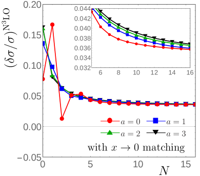
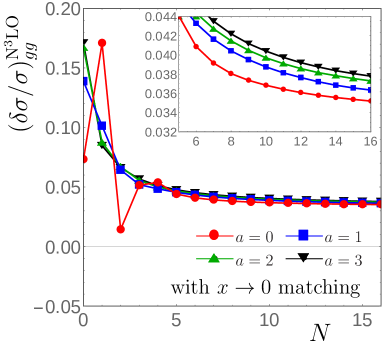
The effect of the matching at N³LO is shown in Fig. 1: the soft expansion tends to a constant towards $x\to 0$ by construction, and cannot reproduce the $\ln^{2}x$-behavior of the exact result. The merging of the two limits is very smooth and suggests that the matched curve is not too far from the full result. Of course, the fact that some coefficients in Eq. (15) are unknown introduces a theoretical uncertainty. However, we observe a change in the final cross section of only about 0.5% when setting $A^{(3,1)}_{gg}=A^{(3,2)}_{gg}$ for a SM Higgs, for example.

Figure 1: Partonic cross section $\hat{\sigma}_{gg}^{t,(3)}/\sigma^{t}_{0}$ in $10^{4}$ according to Eq. (15) as a function of $x=M_{\phi}^{2}/\hat{s}$ with and without matching to the high-energy limit. The order of the soft expansion applied in both cases is $(1-x)^{16}$.

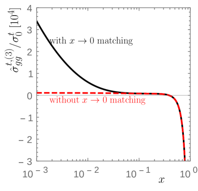
It remains to say that all terms in $1/M_{\text{t}}$ are available including the full $\mu_{\text{F}}$- and $\mu_{\text{R}}$-dependence. As in earlier versions of SusHi, these parameters are accessible through the input parameters SCALES(1) and SCALES(2). Since top-quark mass effects are not known for the N³LO cross section, all settings of GGHMT involving $n=3$ except from GGHMT(30) have no effect in the current version SusHi_1.6.0. The inclusion of $1/M_{\text{t}}$ terms is only available for $M_{\phi}<2M_{\text{t}}$ and the matching to the high-energy limit only in a mass range $M_{\phi}\in\left[100\,\text{GeV},300\,\text{GeV}\right]$.

3.4 Renormalization scale dependence

The renormalization scale ($\mu_{\text{R}}$) dependence of the partonic cross section can be written as

$$\begin{split}\hat{\sigma}_{ij}=\sum_{n\geq 0}\sum_{l=0}^{n}\left(\frac{\alpha_{s}(\mu_{\text{R}})}{\pi}\right)^{n+2}\hat{\kappa}^{(n,l)}_{ij}(\mu_{0})\,l_{\text{R0}}^{l}\,,\end{split}$$ (17)

where $l_{\text{R0}}=2\,\ln(\mu_{\text{R}}/\mu_{0})$, and $\mu_{0}$ is an arbitrary reference scale. The coefficients $\hat{\kappa}^{(n,l)}_{ij}(\mu_{0})$ are explicitly contained in SusHi (for $\mu_{0}=M_{\phi}$). The dependence of the cross section on $\mu_{\text{R}}$ can be studied with SusHi by varying the input parameter SCALES(1), which contains the numerical value for $\mu_{\text{R}}/M_{\phi}$. SusHi will then insert this value into Eq. (17) and convolve the resulting partonic cross section over the PDFs. A decent picture of the $\mu_{\text{R}}$ dependence may require to perform this “standard procedure” ten times or more.

SusHi_1.6.0 provides a considerably faster way to obtain the $\mu_{\text{R}}$ dependence of the cross section by convolving the $\hat{\kappa}^{(n,l)}_{ij}(\mu_{0})$ with the PDFs before varying $\mu_{\text{R}}$,

$$\begin{split}\kappa^{(n,l)}(\mu_{0})=\hat{\kappa}^{(n,l)}_{ij}(\mu_{0})\otimes\tilde{\phi}_{i}\otimes\tilde{\phi}_{j}\,.\end{split}$$ (18)

We will refer to this as the “RGE procedure”. Due to the renormalization group equation

$$\begin{split}\frac{{\rm d}}{{\rm d}\mu_{\text{R}}^{2}}\sigma_{\text{{N${}^{n}$LO}}}={\cal O}(\alpha_{s}^{n+3})=\frac{{\rm d}}{{\rm d}\mu_{\text{R}}^{2}}\hat{\sigma}_{ij,\text{{N${}^{n}$LO}}}\,,\end{split}$$ (19)

which holds both at the partonic and the hadronic level, it suffices to calculate the coefficients $\kappa^{(n,l)}(\mu_{0})$ for $l=0$ and $n\leq 2$ if the N³LO result is requested. SusHi_1.6.0 does this by initially assuming $\mu_{0}/M_{\phi}=\mu_{\text{R}}/M_{\phi}=$ SCALES(1) in Eq. (17). All other coefficients are then determined via the QCD $\beta$ function, defined through

$$\begin{split}\frac{{\rm d}}{{\rm d}\mu_{\text{R}}^{2}}\alpha_{s}(\mu_{\text{R}})=\alpha_{s}(\mu_{\text{R}})\beta(\alpha_{s})\,,\qquad\beta(\alpha_{s})=-\frac{\alpha_{s}}{\pi}\sum_{n\geq 0}\left(\frac{\alpha_{s}}{\pi}\right)^{n}\beta_{n}\,.\end{split}$$ (20)

Explicitly, one finds

$$\begin{split}\kappa^{(1,1)}&=2\,\beta_{0}\,\kappa^{(0,0)}\,,\qquad\kappa^{(2,2)}=\frac{3}{2}\,\beta_{0}\,\kappa^{(1,1)}\,,\qquad\kappa^{(2,1)}=2\,\beta_{1}\,\kappa^{(0,0)}+3\,\beta_{0}\,\kappa^{(1,0)}\,,\\ \kappa^{(3,3)}&=\frac{4}{3}\beta_{0}\,\kappa^{(2,2)}\,,\qquad\kappa^{(3,2)}=\frac{3}{2}\,\beta_{1}\,\kappa^{(1,1)}+2\,\beta_{0}\,\kappa^{(2,1)}\,,\\ \kappa^{(3,1)}&=2\,\beta_{2}\,\kappa^{(0,0)}+3\,\beta_{1}\,\kappa^{(1,0)}+4\,\beta_{0}\,\kappa^{(2,0)}\,.\end{split}$$ (21)

Inserting these coefficients into the hadronic analog of Eq. (17), it is possible to obtain the hadronic cross section at any value of $\mu_{\text{R}}$ without any further numerical integration. Since the $\mu_{\text{R}}$ dependence is typically much larger than the $\mu_{\text{F}}$ dependence for gluon fusion, this feature of SusHi saves a significant amount of computing time when aiming for an estimate of the theoretical uncertainty of the cross section.

Thus, in addition to the usual output file <outfile>, running SusHi_1.6.0 with the standard command

./bin/sushi <infile> <outfile>

will produce an additional file <outfile>_murdep which contains the gluon-fusion cross section for several values of $\mu_{\text{R}}$ in the form

$$\begin{array}[]{rrrrr}\mu_{\text{R}}\text{/GeV}&\sigma_{\text{{LO}}}\text{/pb}&\sigma_{\text{{NLO}}}\text{/pb}&\sigma_{\text{{NNLO}}}\text{/pb}&\sigma_{\text{{N${}^{3}$LO}}}\text{/pb}\end{array}$$ (22)

where all cross sections are evaluated following Eq. (4), i.e. they potentially contain quark-mass effects, SUSY corrections, and/or electroweak effects. The values of $\mu_{\text{R}}$ to be scanned over can be set in <infile> through

⬇

Block SCALES

1 <mu0mh>

102 <min0> <max0> <N>

which will cause SusHi_1.6.0 to evaluate the cross section at $N+1$ equidistant points for $\log\mu_{\text{R}}$ between $\log\mu_{\text{min}}$ and $\log\mu_{\text{max}}$, meaning

$$\begin{split}\mu_{\text{R}}&=\mu_{\text{min}}\left(\frac{\mu_{\text{max}}}{\mu_{\text{min}}}\right)^{i/N}\,,\qquad i\in\{0,1,\ldots,N\}\,.\end{split}$$ (23)

In addition, SusHi_1.6.0 includes a theoretical error estimate on the inclusive cross section into the standard output file <outfile>, given as the maximal and minimal deviation (in pb) within the interval $\mu_{\text{R}}\in[\mu_{1},\mu_{2}]$ from the value at $\mu_{\text{R}}=\mu_{0}$, using the sampled values of $\mu_{\text{R}}$ defined in Eq. (23), and the cross sections at the two boundaries $\mu_{\text{R}}=\mu_{1}$ and $\mu_{2}$. The interval is specified as SCALES(101)={$\mu_{1}/\mu_{0}$,$\mu_{2}/\mu_{0}$} (recall that $\mu_{0}/M_{\phi}=$SCALES(1)); it defaults to $[\mu_{1},\mu_{2}]=[\mu_{0}/2,2\mu_{0}]$.

We remark that this feature works at all perturbative orders through N³LO, for any settings in the blocks GGHMT or GGHSOFT, and for any model under consideration. The only restriction is that all parameters except for the strong coupling constant need to be defined on-shell. If this is not the case, SusHi_1.6.0 will not produce <outfile>_murdep. Note that, due to Eq. (4), the procedure implemented in SusHi_1.6.0 is a slightly refined version of the one described above. In particular, this implies that the NNLO $\mu_{\text{R}}$ dependence is exact, since it is fully determined by the exact NLO cross section $\sigma_{\text{{NLO}}}$. On the other hand, the renormalization-scale dependence at N³LO derived from the RGE procedure inherits whatever approximations were made (or not made) at NNLO. Thus, the results obtained through the standard and the RGE procedure are usually not identical. For example, if one keeps the full $x$-dependence at NNLO, one also obtains the full $x$-dependence of the $\mu_{\text{R}}$-terms at N³LO with the RGE procedure, while the standard procedure would only provide them in the soft expansion.

3.5 Effective Lagrangian - dimension-5 operators

Let us start from a particular well-defined theory TH; in the current version of SusHi, this could be the SM, a general 2HDM, the MSSM, or the NMSSM. We may now include additional gauge invariant dimension-5 operators to TH which couple the neutral Higgs bosons of TH to gluons in the following way:

$$\begin{split}{\cal L}&={\cal L}_{\text{{TH}}}+\sum_{i=1}^{N_{1}}\frac{\alpha_{s}}{12\pi v}c_{5,1i}\,H_{1i}G^{a}_{\mu\nu}G^{a,\mu\nu}+\sum_{i=1}^{N_{2}}\frac{\alpha_{s}}{8\pi v}c_{5,2i}\,H_{2i}G^{a}_{\mu\nu}\tilde{G}^{a,\mu\nu}\,.\end{split}$$ (24)

Here, ${\cal L}_{\text{{TH}}}$ is the Lagrangian of the initial theory TH, $G^{a}_{\mu\nu}$ is the gluonic field strength tensor with color index $a$ and Lorentz indices $\mu$ and $\nu$, and $\tilde{G}_{\mu\nu}^{a}\equiv\varepsilon_{\mu\nu\rho\sigma}G^{a,\rho\sigma}$ is its dual ($\varepsilon^{0123}=+1$). As usual, $\alpha_{s}$ is the strong coupling constant and $v$ the SM Higgs-boson vacuum expectation value, which we express in terms of Fermi’s constant $v=1/\sqrt{\sqrt{2}G_{F}}$. $N_{1}$ and $N_{2}$ are the numbers of CP-even and CP-odd Higgs bosons of the theory, respectively. The particles themselves are generically denoted by $H_{1i}$ and $H_{2i}$ (cf. also Table 1 below).

The $c_{5,ni}$ denote dimensionless Wilson coefficients which are understood as perturbative series in $\alpha_{s}$:

$$c_{5,ni}=\sum_{k=0}^{3}\left(\frac{\alpha_{s}}{\pi}\right)^{k}c_{5,ni}^{(k)}\,.$$ (25)

The normalization is such that $c_{5,ni}^{(0)}=1$ corresponds to the LO contribution of an infinitely heavy up-type quark $u^{\prime}$ with SM-like couplings. The NLO term for a CP-even Higgs in this case would be $c_{5,11}^{(1)}=\tfrac{11}{4}$, etc. In a theory that obeys naturalness, on the other hand, the order of magnitude of the Wilson coefficients would be $c_{5,ni}={\cal O}(v/\Lambda)$, where $\Lambda$ is a scale of physics beyond the SM.

The basic structures for the implementation of the effective Lagrangian in Eq. (24) have already been present in earlier versions of SusHi. The reason for this is that the very same operators result from integrating out the top quark or heavy squarks and gluinos from ${\cal L}_{\text{{TH}}}$. In fact, the NNLO corrections due to top quarks, as well as the NLO corrections due to top, stop, and gluino are evaluated on the basis of these dimension-5 operators.

Thus, SusHi_1.6.0 does not implement any new results; it simply re-uses previously available functions and subroutines in order to extend the gluon-fusion amplitudes to take into account the effect of the additional terms in Eq. (24). The numerical values for the coefficients $c_{5,ni}$ in Eq. (24) are specified through the newly introduced Block DIM5.

<htype>	SM	2HDM/MSSM	NMSSM
11	$H$	$h$	$H_{1}$
12	$-$	$H$	$H_{2}$
13	$-$	$-$	$H_{3}$
21	$A$	$A$	$A_{1}$
22	$-$	$-$	$A_{2}$

Table 1: Assignment of the SusHi input parameter SUSHI(2)=<htype> to the type of Higgs boson in the various models. A dash ($-$) means that the assignment is not meaningful; it will lead to a fatal error in SusHi.

For example, within the MSSM,

⬇

Block DIM5

11 1.00000000E-04 # c5h0

12 4.00000000E-05 # c5H0

21 -3.00000000E-07 # c5A0

corresponds to $c_{5,11}^{(0)}\equiv c_{5,h}^{(0)}=10^{-4}$, $c_{5,12}^{(0)}\equiv c_{5,H}^{(0)}=4\cdot 10^{-5}$, and $c_{5,21}^{(0)}\equiv c_{5,A}^{(0)}=-3\cdot 10^{-7}$. Note that SusHi calculates the cross section of only one particular type of Higgs boson per run (defined in SUSHI(2)), see Ref. [7]. Correspondingly, only the pertinent entry in Block DIM5 will have an effect on the result, the other entries will be ignored. The corrections at higher orders are specified by setting DIM5(<k><ni>) for coefficients $c_{5,ni}^{(k)}$ with $k\geq 1$. At NLO the contribution of an infinitely heavy up-type quark $u^{\prime}$ is thus reproduced by setting DIM5(11)=1 and DIM5(111)=2.75.

The scale dependence of the dimension-5 Wilson coefficient can be derived from the non-renormalization of the trace anomaly term [95, 96, 97, 98],

$$\begin{split}\mu^{2}\frac{{\rm d}}{{\rm d}\mu^{2}}\beta(\alpha_{s})G_{\mu\nu}G^{\mu\nu}\equiv 0\,,\end{split}$$ (26)

where $\beta(\alpha_{s})$ is given in Eq. (20). Since also $\alpha_{s}c_{5,1i}G_{\mu\nu}G^{\mu\nu}$ must be scale invariant, this immediately leads to [10, 99]

$$\begin{split}c_{5,1i}(\mu_{\text{R}})=c_{5,1i}(\mu_{\phi})\frac{(\beta/\alpha_{s})|_{\mu_{\text{R}}}}{(\beta/\alpha_{s})|_{\mu_{\phi}}}\,.\end{split}$$ (27)

Perturbatively, we can write this as

$$c_{5,1i}(\mu_{\text{R}})=\sum_{n\geq 0}\sum_{l=0}^{n}\left(\frac{\alpha_{s}(\mu_{\text{R}})}{\pi}\right)^{n}c_{5,1i}^{(n,l)}(\mu_{\phi})l_{R\phi}^{l}\,,$$ (28)

with $l_{R\phi}=2\ln(\mu_{\text{R}}/\mu_{\phi})$,

$$c_{5,1i}^{(n,0)}=c_{5,1i}^{(n)}(\mu_{\phi})\,,\quad c_{5,1i}^{(n,n)}=0\qquad\forall\ n$$ (29)

and, through NNLO,

$$\begin{split}&c_{5,1i}^{(2,1)}=\beta_{0}c_{5,1i}^{(1,0)}-\beta_{1}c_{5,1i}^{(0,0)}\,,\\ &c_{5,1i}^{(3,2)}=\beta_{0}(\beta_{0}c_{5,1i}^{(1,0)}-\beta_{1}c_{5,1i}^{(0,0)})\,,\quad c_{5,1i}^{(3,1)}=2(\beta_{0}c_{5,1i}^{(2,0)}-\beta_{2}c_{5,1i}^{(0,0)})\,.\end{split}$$ (30)

Setting DIM5(0)=1 makes SusHi evolve the Wilson coefficient perturbatively, i.e. according to Eq. (28); this is the default. On the other hand, one can also employ Eq. (27) for the evolution by setting DIM5(0)=2, similar to the implementation in HIGLU [10]. The evolution can also be switched off (i.e. $c_{5,1i}(\mu_{\text{R}})=c_{5,1i}(\mu_{\phi})$) by setting DIM5(0)=0. The RGE procedure described in the previous section is only applicable for DIM5(0)=1. SusHi will assume the Wilson coefficient provided in the input Block DIM5 to be renormalized at $\mu_{\phi}=M_{\phi}$. The corresponding values at $\mu_{\text{R}}$ (where $\mu_{\text{R}}$ is given in SCALES(1)) are output in Block DIM5OUT.

Moreover, the inclusion of dimension-5 operators is not compatible with the inclusion of $1/M_{\text{t}}$ terms, i.e. SusHi stops if GGHMT(1)$\neq$0 or GGHMT(2)$\neq$0. The LO dependence including quark-mass effects must not be factored out, i.e. SusHi only accepts the setting GGHMT(-1)=-1, in order not to reweight the dimension-5 operator contributions with top-quark mass effects.

We note that through the Block FACTORS, which existed also in earlier versions, SusHi allows to alter the couplings of the Higgs boson to quarks and squarks. Thus, for example additional factors $\kappa_{t}$ and $\kappa_{b}$ for the Higgs-boson coupling to top and bottom quarks can be chosen. In case of the SM the corresponding Lagrangian then takes the following form for the CP-even Higgs boson $H_{11}=H$

$$\mathcal{L}_{\text{{TH}}}\ni-\kappa_{t}\sqrt{2}\frac{M_{\text{t}}}{v}t\bar{t}H-\kappa_{b}\sqrt{2}\frac{M_{\text{b}}}{v}b\bar{b}H\,.$$ (31)

It is therefore easily possible to perform an analysis as presented in Ref. [100] in SusHi, where the dependence of the gluon-fusion cross section on $\kappa_{t}$ and $c_{5,1i}$ is discussed. We will later also focus on this dependence for a very boosted Higgs taking into account the bottom-quark induced contribution in addition. Moreover, by setting the couplings to quarks and gauge bosons to zero through the settings in Block FACTORS and SUSHI(7)=0, respectively, also CP-even or -odd scalars beyond the implemented models can be studied. We will demonstrate this option by providing inclusive cross sections for a scalar with a mass of $750$ GeV at the $13$ TeV LHC in Section 5.4.

4 Heavy-quark annihilation

In this section we shortly comment on the implementation of the total inclusive NNLO Higgs-production cross sections through heavy-quark annihilation, ${\scriptstyle Q}^{\prime}\bar{\scriptstyle Q}\to\phi$, as described in Ref. [30]. Its activation is through the presence of the Block QQH in the input file, which has the following form:

⬇

Block QQH

1 <parton1>

2 <parton2>

11 <v*y>

12 <mu>

Here, <parton1>$\in\{1,\dots,5\}$ denotes the initial-state quark flavor ${\scriptstyle Q}^{\prime}$, and <parton2>$\in\{-1,\dots,-5\}$ the initial-state anti-quark flavor $\bar{\scriptstyle Q}$. <v*y> is the ${\scriptstyle Q}^{\prime}\bar{\scriptstyle Q}\phi$ coupling in the $\overline{\mbox{MS}}$ scheme at scale <mu>$=\mu$/GeV, normalized such that the SM value of the $q\bar{q}H$ coupling is <v*y>$=m_{q}(\mu)$/GeV. For further details regarding the implementation in SusHi_1.6.0 and results we refer to Ref. [30].

If the Block QQH is provided, SusHi will not calculate the gluon-fusion cross section. The calculation of heavy-quark annihilation cross sections is also compatible with cuts on the (pseudo)rapidity or transverse momentum of the Higgs boson up to $\mathcal{O}(\alpha_{s}^{3})$, controlled through the settings in Block DISTRIB. Also $p_{T}$ distributions (DISTRIB(1)=1) can be requested. Since all quarks are assumed massless in this approach, the underlying theory is chirally symmetric. Therefore the results for a scalar and a pseudo-scalar Higgs are identical and the setting of SUSHI(2) is irrelevant. Note also that the collision of an up-type quark with a down-type anti-quark (or vice versa) implies that $\phi$ carries an electric charge. The only model dependence of the ${\scriptstyle Q}^{\prime}\bar{\scriptstyle Q}\phi$ cross section as calculated by SusHi is through the setting of the Yukawa coupling in QQH(11), such that a calculation in the SM-mode is sufficient (SUSHI(1)=0), unless the Higgs mass should be obtained from some external code like FeynHiggs.

Other parameters of the ${\scriptstyle Q}^{\prime}\bar{\scriptstyle Q}\phi$ calculation are determined by the same input values as they are used for the $b\bar{b}\phi$ cross section when no input Block QQH is present. In particular, the perturbative order of ${\scriptstyle Q}^{\prime}\bar{\scriptstyle Q}\phi$ is controlled through SUSHI(6)=$n$, where $n=1,2,3$ results in the LO, NLO, or NNLO prediction, respectively, and the renormalization and factorization scales (relative to $M_{\phi}$) are defined through SCALES(11) and SCALES(12), respectively.

5 Numerical results

This section demonstrates the newly implemented features of SusHi_1.6.0 with the help of exemplary numerical results. We start with a discussion of the convergence of the soft expansion at individual perturbative orders up to N³LO, proceed with top-quark mass effects in the effective field-theory approach, move to the RGE procedure to determine the renormalization-scale dependence, before we use these features to provide a prediction for the cross section of the SM Higgs boson. Finally, we study the effect of higher dimensional operators to the transverse momentum $p_{T}$ of the SM Higgs boson and provide inclusive cross sections for a CP-even scalar with a mass of $750$ GeV. For numerical results concerning heavy-quark annihilation, we refer the reader to Ref. [30].

If not stated otherwise, the setup for the numerical evaluations is as follows: The LHC center-of-mass energy is set to $\sqrt{s}=13$ TeV, and the SM Higgs mass to $M_{\text{H}}=125$ GeV. We employ PDF4LHC15 [101, 102, 103, 104, 105, 106, 107] as parton distribution functions (PDF), where the (n)nlo_mc Monte Carlo is used by default, and the (n)nlo_100 Hessian sets if noted. Since N³LO PDF sets are not available, we use the NNLO set also for the evaluation of the N³LO terms. Nevertheless, in the N³LO calculation, we evolve $\alpha_{s}$ at $4$-loop level; using 3-loop running of $\alpha_{s}$ instead, the final prediction of the cross section for a SM Higgs boson changes at the level of $10^{-5}$. The remaining input follows the recommendation of the LHC Higgs cross section working group, see Ref. [108]. The on-shell charm-quark mass is set to $m_{c}^{\rm OS}=1.64$ GeV, which is the upper edge of the range given in Ref. [108]. The central scale choice for the renormalization and factorization scale is $\mu_{\text{R}}=\mu_{\text{F}}=M_{\text{H}}/2$.

Note that the results of Sections 5.1–5.3 are obtained for a SM Higgs boson. However, SusHi_1.6.0 allows to take into account the effects of N³LO contributions in the heavy-top limit and $1/M_{\text{t}}$ terms to the NNLO contributions for any CP-even Higgs boson in the implemented models, as long as the mass of the Higgs boson under consideration is sufficiently light, i.e. below $2M_{\text{t}}{}$. Effects of dimension-5 operators (see Section 3.5 and 5.4), on the other hand, can be taken into account for any of the neutral Higgs bosons of the implemented models and CP-even and -odd scalars, which couple through dimension-5 operators only.

5.1 Soft expansion up to N³LO

In this section, we study the behavior of the expansion around the “soft limit”, $x\rightarrow 1$, for the gluon-fusion cross section, see also Section 3.1. For the sake of clarity, top-quark mass effects beyond LO will be neglected in this section, although the LO cross section including the full top-quark mass dependence is factored out to all orders (i.e. we set GGHMT(-1)=3, see Section 3.3). In order to discuss the convergence of the soft expansion, we define the quantity

$$\left(\frac{\delta\sigma}{\sigma}\right)^{\text{{N${}^{n}$LO}}}=\frac{\sigma^{t}_{\text{{N${}^{n}$LO}},N,a}}{\sigma^{t}_{\text{{N${}^{n-1}$LO}}}}-1\quad\text{ with }n\geq 1\,,$$ (32)

where $\sigma^{t}_{\text{{N${}^{n}$LO}}}$ has been introduced in Eq. (5). Through ${\cal O}(\alpha_{s}^{n+1})$, the exact $x$-dependence is taken into account. In the highest-order terms, i.e. the terms of order ${\cal O}(\alpha_{s}^{n+2})$ in $\sigma^{t}_{\text{{N${}^{n}$LO}},N,a}$, the soft expansion is applied according to Eq. (5) up to order $(1-x)^{N}$ with $N\leq 16$. All studies in this subsection were performed without matching the cross section to the result at $x\to 0$, i.e., we set GGHMT($n\cdot$10)=0 for $n=1,2,3$.

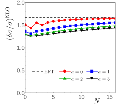
At infinite order of the soft expansion, the value of the parameter $a$ in Eq. (5) is obviously irrelevant. If only a finite number of terms in the expansion is available, the dependence of the result on the parameter $a$ has been studied in detail in Ref. [22]. It was shown that the soft expansion seems to converge particularly well for small, non-negative values of $a$. The differences among the final results for different values of $a$ are smaller at higher orders, as we demonstrate subsequently. One observes that the $\mu_{\text{F}}$-dependent terms of $\hat{\sigma}$ at NLO are polynomial in $x$, which means that they are identical to their soft expansion for $a=0$ once it is taken to sufficiently high order ($N=3$, to be specific). This is no longer true with the choice $a>0$. Let us add that, since the $\mu_{\text{R}}$-dependent terms at NLO are proportional to $\delta(1-x)$, they are the same whether the soft expansion is applied or not.

(a)	(b)

Figure 2: (a) Convergence of the NLO cross section as a function of $N$ for $a=0,1,2,3$ in Eq. (5); (b) Convergence of the NNLO cross section as a function of $N$ for $a=0,1,2,3$ in Eq. (5). In both figures the colors depict $a=0$ (red), $a=1$ (blue), $a=2$ (green), $a=3$ (black). The black, dashed line corresponds to the exact result in the heavy-top limit. The results are obtained for a SM Higgs with $M_{\text{H}}=125$ GeV at the $\sqrt{s}=13$ TeV LHC.

(a)	(b)

Figure 3: (a) Convergence of the N³LO cross section as a function of $N$ for $a=0,1,2,3$ in Eq. (5); (b) Convergence of the gg channel of the N³LO as a function of $N$ for $a=0,1,2,3$ in Eq. (5). A zoom for larger values of $N$ is provided in the upper right corner of the figures. In both figures the colors depict $a=0$ (red), $a=1$ (blue), $a=2$ (green), $a=3$ (black). The results are obtained for a SM Higgs with $M_{\text{H}}=125$ GeV at the $\sqrt{s}=13$ TeV LHC.

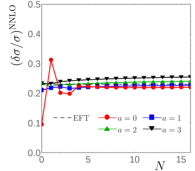
Figs. 2 (a) and (b) show the convergence of the soft expansion at NLO and NNLO, respectively. Both figures also include the result without soft expansion as dashed black line, i.e. where $\sigma^{t}_{\text{{N${}^{n}$LO}},N,a}$ is replaced by $\sigma^{t}_{\text{{N${}^{n}$LO}}}$ in Eq. (32). At NLO, the case $a=0$ appears to be clearly preferable; for larger value of $a$, the soft expansion is further away from the exact $x$-dependence. For $N\geq 9$, the deviation for $a=0$ is less than $2.5$%. It decreases down to $1.3$% at $N=16$, while the result for $a=1$ is still more than $7$% off.

At NNLO, convergence of the soft expansion appears to be a bit faster, with no significant impact of the terms higher than $(1-x)^{6}$ both for $a=0$ and $a=1$. For $N\geq 9$, the result for $a=0$ ($a=1$) approximates the exact $x$-dependence of the correction term to better than $5$% ($2$%) (translating into about $0.9$% ($0.3$%) for the total cross section).

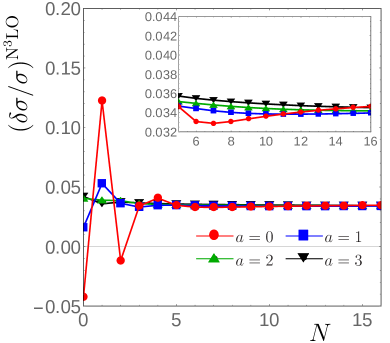
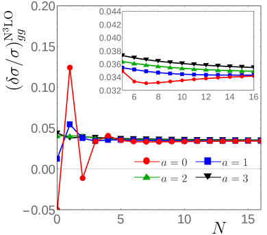
Fig. 3 (a) depicts the convergence of the soft expansion for the cross section at N³LO. Above $N=11$, the spread among the curves for $a=0,1,2,3$ is of the order of $3$% of $\delta\sigma/\sigma$, which means about $0.1$% of the total cross section. For completeness, the same plot for the dominant $gg$ channel alone is shown in Fig. 3 (b). Note that in this case, we only include the $gg$ channel also in the denominator of Eq. (32). At lower orders of the soft expansion, the curve for $a=0$ behaves less smoothly compared to $a\geq 1$; at sufficiently high orders though, all results can be considered consistent with each other at the level of accuracy indicated above.

5.2 Top-quark mass effects through NNLO and matching to the high-energy limit

In this section we comment on top-quark mass effects beyond the heavy-top limit, which can be taken into account in SusHi up to $1/M_{\text{t}}^{10}$ at LO and NLO and up to $1/M_{\text{t}}^{6}$ at NNLO. As already pointed out in Section 3.3, a naive expansion of the partonic cross section in $1/M_{\text{t}}$ breaks down. Thus, in this section, we apply the matching to the high-energy limit as described in Section 3.3, i.e. we set GGHMT($n\cdot$10)=1 for $n=1,2,3$.

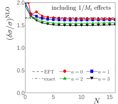
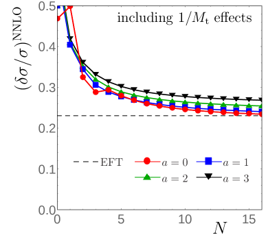
Recall that the matching procedure of Refs. [25, 24] requires the soft expansion of the partonic cross section. Thus before discussing the relevance of the top-quark mass effects, it is necessary to study the convergence of the soft expansion also for these terms. For the result at NLO we can compare to the result in the heavy-top limit, but also to the exact top-quark mass dependence; the difference between these two results is about $1$%. At NNLO, on the other hand, only a comparison to the heavy-top limit is possible. The results are shown in Fig. 4, including terms through $1/M_{\text{t}}^{8}$ at NLO, and through $1/M_{\text{t}}^{4}$ at NNLO (for the $gg$ and the $qg$ channels also $1/M_{\text{t}}^{6}$ terms are implemented in SusHi but provide a negligible contribution, see Fig. 6 below). Following Eq. (32), we keep the exact $x$-dependence one order below to allow for a better comparison with the figures of Section 5.1. At NLO, one observes a nice convergence of the soft expansion to the exact result, provided $a=0$. Terms beyond $(1-x)^{10}$ have only negligible effects on the final result in this case. At NNLO, convergence of the soft expansion is significantly slower, but the available number of terms in this expansion seems sufficient for a prediction of the mass effects with permille level accuracy, provided that $a=0$ is indeed the most reliable choice for the parameter defined in Eq. (5). Fig. 5 shows the N³LO result with matching to the high-energy limit as described in Section 3.3. The convergence of the soft expansion as a function of $N$ is slightly worse compared to the result without matching, but shows a similar behavior as the results at NLO and NNLO depicted in Fig. 4. The correction at $N=16$ is comparable to the result without matching, see Fig. 3.

(a)	(b)

Figure 4: (a) Convergence of the NLO cross section as a function of $N$ for $a=0,1,2,3$ in Eq. (5) with top-quark mass effects up to $1/M_{\text{t}}^{8}$; (b) Convergence of the NNLO cross section as a function of $N$ for $a=0,1,2,3$ in Eq. (5) with top-quark mass effects up to $1/M_{\text{t}}^{4}$. In both figures the colors depict $a=0$ (red), $a=1$ (blue), $a=2$ (green), $a=3$ (black). The black, dashed line corresponds to the exact result in the heavy-top limit, the black, dot-dashed line to the exact result with full top-quark mass dependence (only known at NLO). The results are obtained for a SM Higgs with $M_{\text{H}}=125$ GeV at the $\sqrt{s}=13$ TeV LHC.

(a)	(b)

Figure 5: (a) Convergence of the N³LO cross section as a function of $N$ for $a=0,1,2,3$ in Eq. (5); (b) Convergence of the $gg$ channel of the N³LO as a function of $N$ for $a=0,1,2,3$ in Eq. (5). A zoom for larger values of $N$ is provided in the upper right corner of the figures. In both figures the colors depict $a=0$ (red), $a=1$ (blue), $a=2$ (green), $a=3$ (black). In contrast to Fig. 3 the N³LO result is matched to the high-energy limit. The results are obtained for a SM Higgs with $M_{\text{H}}=125$ GeV at the $\sqrt{s}=13$ TeV LHC.

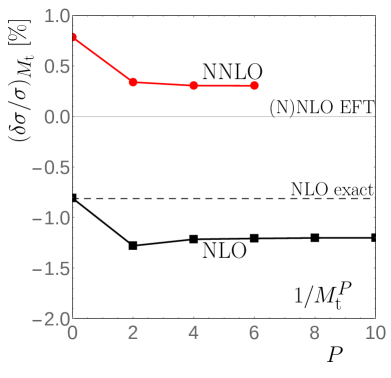
Let us now discuss the top-quark mass effects at different orders $1/M_{\text{t}}^{P}$ in more detail, while applying the soft expansion through $(1-x)^{16}$ with $a=0$ (see Eq. (5)). The result is presented in Fig. 6, where the relative difference

$$\begin{split}\left(\frac{\delta\sigma}{\sigma}\right)_{M_{\text{t}}}=\frac{\sigma_{P}}{\sigma_{\text{htl}}}-1\end{split}$$ (33)

to the heavy-top limit at the corresponding perturbative order is shown. At NLO, $\sigma_{P}$ is obtained by including terms of order $1/M_{\text{t}}^{P}$ in the partonic cross section and matching it to the $x\to 0$ limit (i.e. GGHMT(1)=$P$, GGHMT(10)=1, GGHSOFT(1)={1,16,0}), while $\sigma_{\text{htl}}$ is the heavy-top limit at NLO (i.e. GGHMT(1)=GGHMT(10)=0, GGHSOFT(1)={0,0,0}). In both cases, the value for the cross section provided by SusHi in XSGGHEFF(1) is used.

At NNLO, we use Eq. (4) which corresponds to the SusHi output SUSHIggh(1), neglecting bottom- and charm-quark, and electroweak effects (FACTORS(1)=FACTORS(3)=SUSHI(7)=0). Furthermore, we make sure that only the genuine NNLO effects of the $1/M_{\text{t}}$ terms are shown, by fixing the approximation used at ${\cal O}(\alpha_{s}^{3})$; specifically, we set GGHMT(1)=6, GGHMT(10)=1, and GGHSOFT(1)={1,16,0}, both for $\sigma_{P}$ and $\sigma_{\text{htl}}$. For the $\mathcal{O}(\alpha_{s}^{4})$-terms, we apply the analogous settings of the NLO case described above. I.e., we include terms of order $1/M_{\text{t}}^{P}$ in $\sigma_{P}$ (modulo the restriction to $1/M_{\text{t}}^{4}$ for the pure quark channels, see above), and match them to the $x\to 0$ limit, while we apply the usual heavy-top limit for $\sigma_{\text{htl}}$.

The results are shown in Fig. 6, together with the relative difference of the exact NLO cross section to its heavy-top limit (black dashed). The points at $P=0$ illustrate the effect of using the soft expansion combined with matching to the result at $x=0$, as opposed to keeping the full $x$ dependence (without matching). Both at NLO and NNLO, this effect is obviously larger than the genuine $1/M_{\text{t}}$-terms. This underlines that, as long as one works in a heavy-top approximation, which is strictly valid only for $x>M_{\phi}^{2}/(4M_{\text{t}}^{2})$, the full $x$-dependence is not necessarily an improvement w.r.t. the soft expansion, in particular if additional information like the $x\to 0$ limit is available.

Both at NLO and NNLO, the $1/M_{\text{t}}$ terms exhibit a nice convergence behavior. However, the observation at NLO is that, while the $1/M_{\text{t}}^{0}$ result almost exactly reproduces the full mass dependence after matching to the high-energy limit and employing the soft expansion, including higher-order mass effects moves the approximation away from the exact result. Thus, we cannot expect that their inclusion at NNLO leads to an improved result w.r.t. the heavy-top limit. Nevertheless, we believe that their overall behavior allows to derive an upper bound on the top-mass effects to the heavy-top limit of the order of $1$% [24, 25, 27].

Figure 6: Relevance of $1/M_{\text{t}}^{P}$ terms to the cross section in the heavy-top limit in percent at NLO (black) up to $P=10$ and at NNLO (red) up to $P=6$ with respect to the exact heavy-top limit at the corresponding order. The black, dashed line corresponds to the exact NLO result. The results are obtained for a SM Higgs with $M_{\text{H}}=125$ GeV at the $\sqrt{s}=13$ TeV LHC.

5.3 Cross section prediction for the SM Higgs boson and scale dependence

Having discussed the top-quark mass terms to the NLO and NNLO cross section in the heavy-top limit and the convergence of the soft expansion, we can finally provide a prediction for the cross section of the SM Higgs boson including its scale uncertainty. In this section we make use of the Hessian PDF sets PDF4LHC15_(n)nlo_100. Following the arguments of the preceding sections, the best prediction of SusHi is obtained with the following settings: use the perturbative result through N³LO, i.e. set SUSHI(5)=3; at each order of the effective-theory result, apply the soft expansion through $(1-x)^{16}$ with $a=0$, i.e. set GGHSOFT($n$)={1,16,0} for $n\in\{1,2,3\}$; take into account top-quark mass terms to the predictions of the NLO and NNLO cross sections in the heavy-top limit through the settings GGHMT($n$)=4 for $n\in\{1,2\}$, i.e. $1/M_{\text{t}}^{4}$ terms are taken into account at NLO and NNLO; match to the high-energy limit $x\rightarrow 0$ at NLO, NNLO, and N³LO, i.e. set GGHMT($n\cdot$10)=1 for $n=1,2,3$. The choice of $a=0$ is motivated through the reproduction of the correct scale dependence at NLO and the observations in Section 5. Also note that for all predictions in the effective field-theory approach, we factor out the full top-quark mass dependence, i.e. GGHMT(-1)=3. Finally, we include the electroweak correction factor according to Eq. (4), i.e. we set SUSHI(7)=2. The exact NLO cross section of Eq. (4) contains the contributions from the three heaviest quarks: top, bottom, and charm. The numbers can be reproduced with the input file SM-N3LO_best.in in the example-folder of the SusHi_1.6.0 distribution.

With this setup, we obtain

$$\begin{split}\text{{NNLO}{}}:&\qquad\sigma=43.55\,\text{pb}\pm 4.44\,\text{pb}(\mu_{\text{R}})\,,\\ +\text{{N${}^{3}$LO}}:&\qquad\sigma=45.20\,\text{pb}\pm 1.61\,\text{pb}(\mu_{\text{R}})\,,\\ +\text{$1/M_{\text{t}}$ effects at {NLO}{} and {NNLO}{}}\,\,&\\ +\text{matching ($x\to 0$) at {NLO}{}, {NNLO}{} and {N${}^{3}$LO}}:&\qquad\sigma=45.80\,\text{pb}\pm 1.87\,\text{pb}(\mu_{\text{R}})\,,\\ +\text{electroweak corrections}:&\qquad\sigma=48.28\,\text{pb}\pm 1.97\,\text{pb}(\mu_{\text{R}})\,,\end{split}$$ (34)

where the uncertainty $\pm\Delta(\mu_{\text{R}})$ only takes into account the renormalization-scale dependence. Here, $\Delta(\mu_{\text{R}})$ is the maximum deviation of the cross section within the interval $\mu_{\text{R}}/M_{\text{H}}\in[1/4,1]$ from the value at $\mu_{\text{R}}=M_{\text{H}}/2$. Each line of Eq. (34), including the uncertainty, has been obtained in a single run of SusHi, which takes a few seconds on a modern desktop computer. The final result is perfectly consistent within its uncertainties with the prediction $48.58\,\text{pb}\pm 1$ pb($\mu_{\text{R}}$) given in Ref. [22] and the result $48.1\,\text{pb}\pm 2.0$ pb (without resummation) employing the Cacciari-Houdeau Bayesian approach [109] to estimate higher unknown orders presented in Ref. [18]. We note that the result of Ref. [22] was computed with the NNLO PDF set at all orders, whereas we employ the NLO PDF set for the NLO terms in Eq. (4). If we employ PDF4LHC15_nnlo_100 instead at all orders, we obtain $48.37$ pb. Other uncertainties need to be added as described in Refs. [6, 22].

(a)	(b)

Figure 7: (a) LO (red, dotted), NLO (green, dashed), NNLO (blue, dot-dashed) and N³LO (black, solid) gluon-fusion cross section in pb (see Eq. (4)) as a function of $\mu_{\text{R}}/M_{\text{H}}$ (obtained in a single run); (b) Best prediction cross section in pb as a function of $\mu_{\text{F}}/M_{\text{H}}$ (together with $\mu_{\text{R}}=M_{\text{H}}/2$) (blue) and $\mu_{\text{F}}/M_{\text{H}}=\mu_{\text{R}}/M_{\text{H}}$ (red) and $\mu_{\text{R}}/M_{\text{H}}$ (together with $\mu_{\text{F}}=M_{\text{H}}/2$) (black). Each curve is shown twice, once for $a=0$ (solid) and $a=1$ (dashed) in the soft expansion at N³LO. The dotted, thin black line depicts the N³LO result from (a). Both figures are obtained for a SM Higgs with $M_{\text{H}}=125$ GeV at the $\sqrt{s}=13$ TeV LHC.

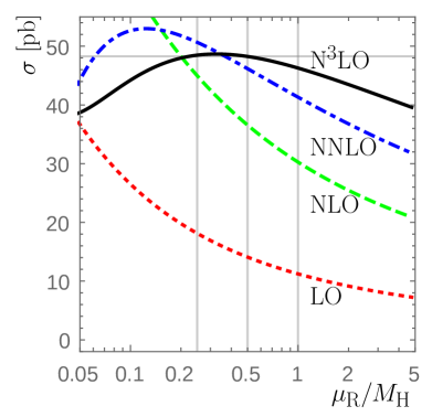
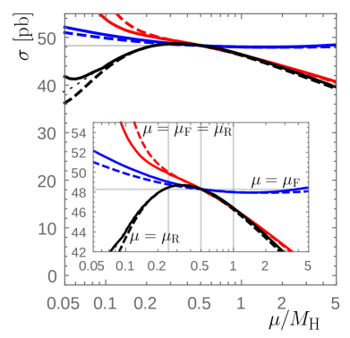
Running the input file SM-N3LO_best.in also generates a file including the renormalization-scale dependence. Its content is shown in Fig. 7 (a). The dependence clearly reduces successively from NLO to N³LO. Note that at each order we follow Eq. (4) and thus include the electroweak correction factor beyond LO. The flat behavior around $\mu_{\text{R}}=M_{\text{H}}/2$ leads to a highly asymmetric scale variation around the central value, suggesting a symmetrization of the corresponding uncertainty band as done in Eq. (34). As explained in Section 3.4, the $\mu_{\text{R}}$ dependence obtained through the RGE procedure at NⁿLO is as precise as the calculation at N^n-1LO, while in the standard procedure (by manually varying SCALES(1)), its precision is determined by the NⁿLO calculation. We show the result of the standard procedure in Fig. 7 (b) (black lines). In addition, the $\mu=\mu_{\text{F}}$ dependence for $\mu_{\text{R}}=M_{\text{H}}/2$ (blue) and the combined $\mu=\mu_{\text{F}}=\mu_{\text{R}}$ dependence (red) are shown. In each case, the solid and dashed line corresponds to setting $a=0$ and $a=1$ in Eq. (5), respectively. The differences between these two cases, as well as between the standard and the RGE procedure are small, except for small values of $\mu$. We also observe that the behavior at low values of $\mu$ in Fig. 7 (b) is dependent on the soft expansion and the matching performed at NLO and NNLO. However, within the interval $\mu\in\left[M_{\text{H}}/4,M_{\text{H}}\right]$ which we use for the uncertainty determination, the agreement is good.

5.4 Dimension $5$ operators

In order to study the effect of the dimension-5 operators, it is helpful to consider the fraction of events where the SM Higgs boson is produced at transverse momenta above a certain value $p_{T}^{\text{cut}}$. We define

$$\begin{split}R(p_{T}^{\text{cut}})=\frac{1}{\sigma^{\text{tot}}}\sigma(p_{T}^{\text{cut}})\quad\text{with}\quad\sigma(p_{T}^{\text{cut}})=\int_{p_{T}>p_{T}^{\text{cut}}}{\rm d}p_{T}\frac{{\rm d}\sigma}{{\rm d}p_{T}}\,,\end{split}$$ (35)

where $\sigma\equiv\sigma_{ni}(c_{5,ni})$ denotes the cross section for the production of a Higgs boson $H_{ni}$ within the theory defined by Eq. (24), and follow the numerical setup described at the beginning of Section 5. However, we do not take into account charm-quark and electroweak contributions and choose a $p_{T}$-dependent renormalization and factorization scale for the result presented in Fig. 10. If not stated otherwise, the relative Yukawa couplings to top- and bottom quarks are set to one, i.e. we discuss the specific model TH with additional dimension-5 operator. In the subsequent NLO analysis, we set $c_{5}^{(1)}=\tfrac{11}{4}c_{5}^{(0)}$, i.e. our dimension-5 operator assumes the same (rescaled) NLO correction as for the top-quark induced Wilson coefficient.

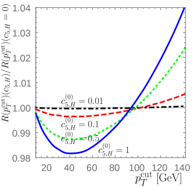
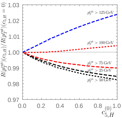
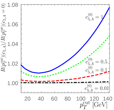
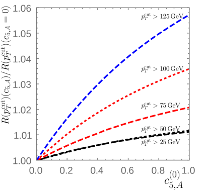
The ratio $R(p_{T}^{\text{cut}})$ of Eq. (35) is shown in Fig. 8 for the SM Higgs boson as a function of (a) $p_{T}^{\text{cut}}$ for various values of $c_{5,H}^{(0)}$, and (b) $c_{5,H}^{(0)}$ for various values of $p_{T}^{\text{cut}}$. Similarly, Fig. 9 shows the ratio for a CP-odd Higgs boson with mass $125$ GeV. For Fig. 8 (a) and Fig. 9 (a), $\sigma^{\text{tot}}$ is chosen such that each $R(p_{T}^{\text{cut}})$ is normalized to its NLO inclusive cross section. For Fig. 8 (b) and Fig. 9 (b), $\sigma^{\text{tot}}=\sigma(p_{T}^{\text{cut}})$ for $c_{5}=0$ to ensure that all curves start at one. The minima, which are clearly visible around $p_{T}^{\text{cut}}=50$ GeV, are induced by the negative interference with the bottom-quark induced contributions to gluon fusion, which turns into a positive interference for higher values of $p_{T}^{\text{cut}}$. Accordingly, these minima affect also the dependence on $c_{5}$ in Fig. 8 (b) and Fig. 9 (b), i.e. the lowest curve is obtained for a value of $p_{T}^{\text{cut}}$ around $40$ GeV. Apart from the impact on the inclusive cross section, the point-like interaction encoded in the coefficient $c_{5}$ thus distorts the shape of the $p_{T}$ distributions with respect to the loop-induced massive top- and bottom-quark contributions, as expected.

(a)	(b)

Figure 8: (a) Ratio of $R(p_{T}^{\text{cut}})$ with different $c_{5,H}^{(0)}$ (see figure) and $R(p_{T}^{\text{cut}})$ with $c_{5,H}=0$ as a function of $p_{T}^{\text{cut}}$ in GeV; (b) Ratio of $R(p_{T}^{\text{cut}})$ and $R(p_{T}^{\text{cut}})$ with $c_{5,H}=0$ as a function of $c_{5,H}^{(0)}$ for different $p_{T}^{\text{cut}}$ (see figure). In both figures we set $c_{5,A}^{(1)}=\tfrac{11}{4}c_{5,A}^{(0)}$. Both figures are obtained for a CP-even SM Higgs with $M_{\text{H}}=125$ GeV at the $\sqrt{s}=13$ TeV LHC.

(a)	(b)

Figure 9: (a) Ratio of $R(p_{T}^{\text{cut}})$ with different $c_{5,A}^{(0)}$ (see figure) and $R(p_{T}^{\text{cut}})$ with $c_{5,A}=0$ as a function of $p_{T}^{\text{cut}}$ in GeV; (b) Ratio of $R(p_{T}^{\text{cut}})$ and $R(p_{T}^{\text{cut}})$ with $c_{5,A}=0$ as a function of $c_{5,A}^{(0)}$ for different $p_{T}^{\text{cut}}$ (see figure). In both figures we set $c_{5,A}^{(1)}=\tfrac{11}{4}c_{5,A}^{(0)}$. Both figures are obtained for a CP-odd Higgs with $m_{A}=125$ GeV at the $\sqrt{s}=13$ TeV LHC.

Following the study performed in Ref. [100], we now work out the dependence of the cross section with a minimal cut on $p_{T}$ on the factors $\kappa_{t}$ and $c_{5,H}^{(0)}$ for the SM Higgs boson. In addition, we include the dependence on the bottom-quark induced contribution through the factor $\kappa_{b}$, since the latter is non-negligible for $p_{T}^{\text{cut}}<200$ GeV. For this study we also choose $p_{T}$-dependent renormalization and factorization scales $\mu_{\text{R}}=\mu_{\text{F}}=\sqrt{M_{\text{H}}^{2}+p_{T}^{2}}/2$, which is possible through the setting SCALES(3)=1. We define $\tilde{\sigma}(p_{T}^{\text{cut}})$, which just includes the top-quark induced contribution, i.e. we set $\kappa_{t}=1$ and $c_{5,H}=\kappa_{b}=0$, and then perform a fit of

$$\frac{\sigma(p_{T}^{\text{cut}})}{\tilde{\sigma}(p_{T}^{\text{cut}})}=(\kappa_{t}+c_{5,H}^{(0)})^{2}+\delta\kappa_{t}c_{5,H}^{(0)}+\epsilon(c_{5,H}^{(0)})^{2}+\delta_{bt}\kappa_{b}\kappa_{t}+\delta_{bg}\kappa_{b}c_{5,H}^{(0)}+\epsilon_{b}\kappa_{b}^{2}\,,$$ (36)

where we set $c_{5,H}^{(1)}=\tfrac{11}{4}c_{5,H}^{(0)}$ and $\delta$ and $\epsilon$ are defined identically to Ref. [100]. In addition, however, we include the bottom-quark induced contribution, which is understood as pure correction entering through $\delta_{bg}$, $\delta_{bt}$, and $\epsilon_{b}$. The values for $\delta$ and $\epsilon$ coincide at the percent level with the values of Table $1$ in Ref. [100], where for completeness we note that our calculation also includes the $qq$ induced contribution to gluon fusion. For our numerical setup we show the dependence of the five correction factors on the lower cut $p_{T}^{\text{cut}}$ in Fig. 10.

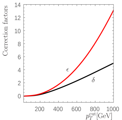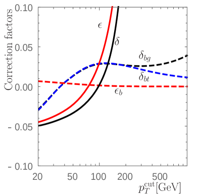(a)	(b)

Figure 10: (a) Correction factors $\delta$, $\epsilon$ as a function of the lower cut $p_{T}^{\text{cut}}$ in GeV and in addition (b) $\delta_{bg}$, $\delta_{bt}$ and $\epsilon_{b}$ as a function of $p_{T}^{\text{cut}}$. Both figures are obtained for a SM Higgs with $M_{\text{H}}=125$ GeV at the $\sqrt{s}=13$ TeV LHC.

As can be seen in Fig. 10 (a), the larger the lower cut $p_{T}^{\text{cut}}$, the more the degeneracy between $\kappa_{t}$ and $c_{5,H}$, which are indistinguishable in the inclusive cross section, is broken. On the other hand Fig. 10 (b) points out that for low $p_{T}^{\text{cut}}<200$ GeV bottom-quark induced contributions should also be taken into account. The interferences of the latter with the top-quark induced contributions on the one hand and with the effective coupling $c_{5,H}$ on the other hand, encoded in $\delta_{bt}$ and $\delta_{bg}$, are identical only for low $p_{T}^{\text{cut}}$. We note that the cross section prediction for the SM Higgs boson of course should include the full correction by bottom quarks given by $\delta_{bt}$ and $\epsilon_{b}$. For completeness we partially also reproduced Fig. $2$ of Ref. [100], which illustrates the disentanglement of the degeneracy between $\kappa_{t}$ and $c_{5,H}$.

As a last example we discuss the calculation of the gluon-fusion cross section for an arbitrary scalar, which couples to gluons through an effective operator $c_{5}^{(0)}=1$ only. Motivated by the background deviation in the diphoton channel at $750$ GeV in both LHC experiments [110, 111], we choose the mass of the scalar to be $m_{X}=750$ GeV. We pick an input file for the SM, set the SM Higgs-boson mass to $M_{\text{H}}{}=750$ GeV, include a dimension-5 operator through DIM5(11)=1, but set the SM Higgs-boson couplings to quarks and gauge bosons to zero in Block FACTORS and through SUSHI(7)=0. The results are shown in Tab. 2. We include the renormalization scale uncertainty $\pm\Delta(\mu_{\text{R}})$, which was obtained simultaneously. Again $\Delta(\mu_{\text{R}})$ is the maximum deviation of the cross section within the interval $\mu_{\text{R}}\in[1/4,1]m_{X}$ and $\mu_{\text{R}}\in[1/2,2]m_{X}$ for the central scale choices $\mu_{\text{R}}=\mu_{\text{F}}=m_{X}/2$ and $\mu_{\text{R}}=\mu_{\text{F}}=m_{X}$, respectively. For this purpose the Wilson coefficient is evolved perturbatively, i.e. DIM5(0)=1. At N³LO the soft expansion is performed up to $(1-x)^{16}$ with $a=0$. The matching to the high-energy limit, $x\to 0$, is not applied. Similar to the SM Higgs boson we observe a good convergence of the perturbative series with a renormalization scale uncertainty of less than $\pm 1.3$ and $\pm 2.9$% at N³LO QCD for the central scale choices $\mu_{\text{R}}=\mu_{\text{F}}=m_{X}/2$ and $\mu_{\text{R}}=\mu_{\text{F}}=m_{X}$, respectively.

$\sigma(gg\to X)$ [fb]	$\mu_{\text{R}}=\mu_{\text{F}}=m_{X}/2$	$\mu_{\text{R}}=\mu_{\text{F}}=m_{X}$
LO	$246.2\pm 52.8$	$185.8\pm 36.0$
NLO	$368.7\pm 43.1$	$316.3\pm 39.1$
NNLO	$410.0\pm 19.1$	$384.9\pm 24.0$
N3LO	$414.6\pm 5.4$	$407.2\pm 11.7$

Table 2: Inclusive gluon-fusion cross section in fb for a CP-even scalar with mass $m_{X}=750$ GeV, which couples to gluons through $c_{5}^{(0)}=1$ only. The results are given at different orders N^kLO, $k=0,1,2,3$, in QCD for the $\sqrt{s}=13$ TeV LHC for two renormalization and factorization scale choices. The depicted uncertainty is the renormalization-scale uncertainty $\pm\Delta(\mu_{\text{R}})$.

6 Conclusions

We presented the new features implemented in version 1.6.0 of the code SusHi. Aside from the implementation of heavy-quark annihilation, many new features aim at the improvement of the gluon-fusion cross-section prediction and its associated uncertainty estimate. In particular, SusHi now provides the soft expansion around the threshold of Higgs production and the matching to the high-energy limit for CP-even Higgs bosons, at NLO, NNLO and N³LO QCD. Top-quark mass effects beyond the usual infinite top-mass limit can be taken into account at NLO and NNLO. We investigated the relevance of these effects for a SM-like Higgs boson with a mass of $125$ GeV and provide a prediction of the corresponding gluon-fusion cross section at the LHC with a center-of-mass energy of $13$ TeV. Both for CP-even and -odd Higgs bosons, SusHi now calculates the renormalization-scale uncertainty simultaneously to the calculation of the gluon-fusion cross section at the central scale. Moreover, the effects of dimension-5 operators can be studied in any model currently supported by SusHi. We showed how the degeneracy between the top-quark mass contribution and a point-like dimension-5 operator contribution can be broken at large values of the transverse momentum of a Higgs boson with mass $125$ GeV. The implementation of arbitrary dimension-5 operators is also particularly suited for the study of new CP-even and -odd scalars beyond the implemented models. We showed the convergence of the perturbative series for the inclusive gluon-fusion cross section of a scalar with mass $750$ GeV at the $13$ TeV LHC.

Our description and the subsequent appendix include examples how the user can control the new features through the setting of blocks in the input file of SusHi. Example input files are contained in the example-folder of the current SusHi release to be found at [8].

Appendix A Example input

In this appendix we present exemplary input blocks, which control features that have been added to SusHi since its original release described in Ref. [7] (version 1.0.0). This includes the features described in the main text of this paper, but also others like the introduction of the NMSSM [9] and the 2HDM, or the calculation of the Higgs cross section in general heavy-quark annihilation through NNLO [30]. For a complete up-to-date manual of SusHi, we refer the reader to Ref. [112].

We begin with the main Block SUSHI which may look as follows:

⬇

Block SUSHI

1 0 # Chosen model: 0=SM, 1=MSSM, 2=2HDM, 3=NMSSM

2 11 # 11/12/13=scalar, 21/22=pseudo-scalar

3 0 # Particle collider: 0=pp, 1=ppbar

4 1.3E+04 # center-of-mass energy in GeV

5 3 # Order for ggh

6 2 # Order for bbh

7 2 # Electroweak contributions to ggh

19 1 # 0 = silent mode of SusHi, 1 = normal output

20 10 # ggh@nnlo subprocesses: 0=all, 10=ind. contributions

21 0 # bbh@nnlo subprocesses: 0=all

SUSHI(1) controls the physics model, SUSHI(2) the Higgs boson under consideration. In contrast to the original release with the 2HDM-adapted options SUSHI(2)$\in${0,1,2} for the light, the pseudo-scalar and the heavy Higgs boson, respectively, the Higgs bosons are now defined in the more general NMSSM-framework, where SUSHI(2)$\in\{$11,12,13$\}$ denote the CP-even Higgs bosons $\{H_{1},H_{2},H_{3}\}$, and SUSHI(2)$\in\{$21,22$\}$ the CP-odd Higgs bosons $\{A_{1},A_{2}\}$. If SUSHI(1)=0, $H_{1}$ assumes the role of the SM Higgs boson, while $A_{1}$ is a hypothetical pseudo-scalar with “SM-like” couplings (see, e.g., Ref. [113] for details). If SUSHI(1)$\in\{$1,2$\}$, then $H_{1}=h$ and $H_{2}=H$ are the light and the heavy CP-even Higgs boson, and $A_{1}=A$ is the CP-odd Higgs boson of the MSSM or the 2HDM.

SUSHI(5) now allows for the settings SUSHI(5)=3, activating the N³LO QCD top-quark contributions as discussed in this paper, and SUSHI(5)=12 for the inclusion of approximate NNLO stop contributions as described in Ref. [78] (see also Ref. [77]). Other new options are set in SUSHI($n$) with $n\geq 10$: SUSHI(19) controls the screen output verbosity of SusHi, while SUSHI(20) and SUSHI(21) allow to display the individual subchannels in the calculations of gluon-fusion and bottom-quark annihilation, respectively.

We continue with a description of the input blocks to control the effects described in this paper. For this purpose we consider the input file SM-N3LO_best.in, which contains new input entries in Block GGHMT, Block GGHSOFT, and Block SCALES. The Block GGHMT controls top-quark mass effects in the calculation of the gluon fusion cross section and has the following entries:

⬇

Block GGHMT

-1 3 # factor out exact LO result at LO(=0)/NLO(=1)/etc.

0 -1 # expand through 1/mt^n at LO [-1=exact]

1 4 # expand through 1/mt^n at NLO

11 4 # expand gg through 1/mt^n at NLO

12 4 # expand qg through 1/mt^n at NLO

13 4 # expand qqbar through 1/mt^n at NLO

2 4 # expand through 1/mt^n at NNLO

21 4 # expand gg through 1/mt^n at NNLO

22 4 # expand qg through 1/mt^n at NNLO

23 4 # expand qqbar through 1/mt^n at NNLO

24 4 # expand qq through 1/mt^n at NNLO

25 4 # expand qqprime through 1/mt^n at NNLO

3 0 # expand through 1/mt^n at N3LO (more not implemented)

10 1 # [0/1]: do not/match to high energy limit at NLO

20 1 # [0/1]: do not/match to high energy limit at NNLO

30 1 # [0/1]: do not/match to high energy limit at N3LO

In this example, we factor out the the LO top-quark mass dependence through the first setting. The parameter GGHMT(0) is only of relevance for GGHMT(-1)=-1 (meaning that the LO top-quark mass dependence is not factored out) and allows to control the top-quark mass terms in the LO contribution in this case. Beyond LO, we take into account the first four terms in the expansion in $1/M_{\text{t}}$ in all channels. Finally, through GGHMT($n\cdot 10$)=1 with $n\geq 1$, we match to the high-energy limit at each order beyond LO.

The block Block GGHSOFT activates the soft expansion around the threshold of Higgs production through GGHSOFT(n,1)=1 with $n\in\{1,2,3\}$ and performs it up to $(1-x)^{16}$ with $a=0$, see Eq. (5):

⬇

Block GGHSOFT # parameters for soft expansion

1 1 16 0 # NLO [0/1=n/y] [order] sig(x)/x^[n]

2 1 16 0 # NNLO [0/1=n/y] [order] sig(x)/x^[n]

3 1 16 0 # N3LO [0/1=n/y] [order] sig(x)/x^[n]

Let us next consider the new settings in Block SCALES:

⬇

Block SCALES

1 5.00000000E-01 # Renormalization scale muR/mh for ggh

2 5.00000000E-01 # Factorization scale muF/mh for ggh

101 5.00E-01 2.00E+00 # min and max for muR uncertainty around SCALES(1)

102 1.00E-01 1.00E+01 100 # min/max/steps for table of muR variation

11 1.00000000E+00 # Renormalization scale muR/mh for bbh

12 2.50000000E-01 # Factorization scale muF/mh for bbh

Entry SCALES(101) defines the interval of $\mu_{\text{R}}$ relative to the central scale given in SCALES(1), which SusHi uses to determine the renormalization scale uncertainty of the gluon fusion cross section following Section 3.4. Thus, in this example, the $\mu_{\text{R}}$ uncertainty is obtained from a variation of $\mu_{\text{R}}$ within the interval $\mu_{\text{R}}\in[0.5,2]\cdot 0.5\cdot M_{\text{H}}$. The minimal and maximal values of $\mu_{\text{R}}$ with respect to the central scale choice relevant for the output file <outfile>_murdep are specified in SCALES(102). In the example, the cross sections at 100 $\mu_{\text{R}}$ values within $[1/10,10]\cdot 0.5\cdot M_{\text{H}}$ will be printed in the additional output file. Finally, note that the renormalization and factorization scales for bottom-quark annihilation can be set independently in SCALES(11) and (12), which is possible since SusHi release 1.2.0.

For the discussion of dimension-5 operators we add an example of an arbitrary scalar $\phi$ coupling to gluons, similar to the one in the last paragraph of Section 5.4.

⬇

Block DIM5

0 1 # Running of DIM5 operators 0=off/1=pert./2=res.

11 1.00000000E+00 # LO coeff of dim-5 operator

111 0.00000000E+00 # NLO coeff of dim-5 operator

211 0.00000000E+00 # NNLO coeff of dim-5 operator

311 0.00000000E+00 # N3LO coeff of dim-5 operator

We thus consider a CP-even Higgs boson through SUSHI(2)=11 and control its coupling to gluons through DIM5($n\cdot$100$+$11) with $n\in\{0,1,2,3\}$. The setting DIM5(0)=1 evolves the dimension-5 operator perturbatively, and through DIM5(11)=1 we only fix the lowest order contribution of the dimension-5 operator at the scale $M_{\phi}$ to a non-vanishing value. Higher order contributions will be generated through the perturbative running and can be taken from the output Block DIM5OUT in the output file.

Next we display an example of the calculation of the cross section $c\bar{c}\to H$ in the SM through the settings in Block QQH, where apart from the incoming parton types also the Yukawa coupling in GeV and the input scale of the Yukawa coupling in GeV have to be specified:

⬇

Block QQH

1 4 # parton 1 = c

2 -4 # parton 2 = cbar

11 1.27500000E+00 # Yukawa coupling

12 1.27500000E+00 # renorm.-scale for input Yuk.-coupl.

Let us next discuss the access to new physics models within SusHi. Since SusHi_1.0.2, calculations in the CP-conserving 2HDM can be performed. Release 1.1.1 introduced a link to the external code 2HDMC [88]. The input of the 2HDM closely resembles the SM input. The user has to specify the Higgs under consideration using SUSHI(2)$\in\{$11,12,21$\}$ for the light, the heavy, and the pseudo-scalar Higgs, respectively. Moreover, the corresponding Higgs mass has to be given in Block MASS together with the Higgs mixing angle $\alpha$ in Block ALPHA and the ratio of the vacuum expectation values $\tan\beta$ in Block MINPAR. The different types of the 2HDM as discussed in Ref. [114] can be distinguished in Block 2HDM:

⬇

Block 2HDM # 2HDM version according to Ref. [114]

2 # (1=Type I,2=Type II,3=Flipped,4=Lepton Specific)

Block MINPAR

3 5.00000000E+00 # tanb

Block ALPHA

-5.00000000E-01 # mixing in CP-conserving Higgs sector

Block MASS

25 1.25000000E+02 # Higgs mass h

35 1.50000000E+02 # Higgs mass H

36 3.00000000E+02 # Pseudoscalar Higgs mass A

The link to 2HDMC allows the user to provide the 2HDM input parameters in Block 2HDMC either in the $\lambda$ basis, the physical basis, or the H2 basis. For details we refer to the 2HDMC manual. Block 2HDMC makes the blocks 2HDM, MINPAR, ALPHA and MASS obsolete. Example input files are provided in the example-folder of the current SusHi distribution. For example, in case of the $\lambda$ basis, the relevant block takes the form:

⬇

Block 2HDMC # 2HDMC (Ref. [88])

1 1 # 2HDMC key, 1=lambda basis, 2=physical basis, 3=H2 basis

2 2 # 2HDM version type

3 1.00000000E+01 # tan(beta)

4 1.00000000E+02 # m12

11 1.00000000E-01 # lambda1

12 2.00000000E-01 # lambda2

13 3.00000000E-01 # lambda3

14 4.00000000E-01 # lambda4

15 5.00000000E-01 # lambda5

16 0.00000000E-01 # lambda6

17 0.00000000E-01 # lambda7

Since version 1.5.0, SusHi includes also the NMSSM [115]. For the corresponding input blocks we refer to Ref. [9] (note, however, a change in the convention for Block NMAMIX [115]). Contrary to the MSSM and the 2HDM, no link to an external code is provided, such that the NMSSM Higgs sector has to be specified completely in the input file. This involves the Higgs masses in Block MASS as well as the Higgs mixing in the CP-even sector in Block NMHMIX and the CP-odd sector in Block NMAMIX.

SusHi_1.5.0 also introduced the Block FEYNHIGGSFLAGS, which allows to control the various options of a FeynHiggs [84, 85, 86, 87] run in the MSSM. The number of arguments depends on the FeynHiggs version, please consider the MSSM input and output files in the example-folder of each SusHi release. We generally provide input files for all models and links to external codes in the folder example, which is part of each SusHi release. We thus encourage the user to start his/her considerations with an example input file.

References

- [1] G. Aad et al. [ATLAS Collaboration], Phys. Lett. B 716 (2012) 1 [arXiv:1207.7214].
- [2] S. Chatrchyan et al. [CMS Collaboration], Phys. Lett. B 716 (2012) 30 [arXiv:1207.7235].
- [3] S. Dittmaier et al. [LHC Higgs Cross Section Working Group Collaboration], “Handbook of LHC Higgs Cross Sections: 1. Inclusive Observables,” arXiv:1101.0593.
- [4] S. Dittmaier et al. [LHC Higgs Cross Section Working Group Collaboration], “Handbook of LHC Higgs Cross Sections: 2. Differential Distributions,” arXiv:1201.3084.
- [5] S. Heinemeyer et al. [LHC Higgs Cross Section Working Group Collaboration], “Handbook of LHC Higgs Cross Sections: 3. Higgs Properties,” arXiv:1307.1347.
- [6] D. de Florian et al. [LHC Higgs Cross Section Working Group Collaboration], “Handbook of LHC Higgs Cross Sections: 4. Deciphering the Nature of the Higgs Sector,” arXiv:1610.07922.
- [7] R. V. Harlander, S. Liebler and H. Mantler, Comput. Phys. Commun. 184 (2013) 1605 [arXiv:1212.3249].
- [8] Webpage of SusHi: http://sushi.hepforge.org.
- [9] S. Liebler, Eur. Phys. J. C 75 (2015) 5, 210 [arXiv:1502.07972].
- [10] M. Spira, hep-ph/9510347.
- [11] E. Bagnaschi, G. Degrassi, P. Slavich and A. Vicini, JHEP 1202 (2012) 088 [arXiv:1111.2854].
- [12] C. Anastasiou, S. Buehler, F. Herzog and A. Lazopoulos, JHEP 1112 (2011) 058 [arXiv:1107.0683].
- [13] C. Anastasiou, S. Bucherer and Z. Kunszt, JHEP 0910 (2009) 068 [arXiv:0907.2362].
- [14] S. Catani and M. Grazzini, Phys. Rev. Lett. 98 (2007) 222002 [hep-ph/0703012].
- [15] S. Catani and M. Grazzini, PoS RADCOR 2007 (2007) 046 [arXiv:0802.1410].
- [16] R. D. Ball, M. Bonvini, S. Forte, S. Marzani and G. Ridolfi, Nucl. Phys. B 874 (2013) 746 [arXiv:1303.3590].
- [17] M. Bonvini, R. D. Ball, S. Forte, S. Marzani and G. Ridolfi, J. Phys. G 41 (2014) 095002 [arXiv:1404.3204].
- [18] M. Bonvini, S. Marzani, C. Muselli and L. Rottoli, JHEP 1608 (2016) 105 [arXiv:1603.08000].
- [19] C. Anastasiou, C. Duhr, F. Dulat, E. Furlan, T. Gehrmann, F. Herzog and B. Mistlberger, JHEP 1503 (2015) 091 [arXiv:1411.3584].
- [20] C. Anastasiou, C. Duhr, F. Dulat, F. Herzog and B. Mistlberger, Phys. Rev. Lett. 114 (2015) 212001 [arXiv:1503.06056].
- [21] C. Anastasiou, C. Duhr, F. Dulat, E. Furlan, F. Herzog and B. Mistlberger, JHEP 1508 (2015) 051 [arXiv:1505.04110].
- [22] C. Anastasiou, C. Duhr, F. Dulat, E. Furlan, T. Gehrmann, F. Herzog, A. Lazopoulos and B. Mistlberger, JHEP 1605 (2016) 058 [arXiv:1602.00695].
- [23] S. Marzani, R. D. Ball, V. Del Duca, S. Forte and A. Vicini, Nucl. Phys. B 800 (2008) 127 [arXiv:0801.2544].
- [24] R. V. Harlander, H. Mantler, S. Marzani and K. J. Ozeren, Eur. Phys. J. C 66 (2010) 359 [arXiv:0912.2104].
- [25] R. V. Harlander and K. J. Ozeren, JHEP 0911 (2009) 088 [arXiv:0909.3420].
- [26] R. V. Harlander and K. J. Ozeren, Phys. Lett. B 679 (2009) 467 [arXiv:0907.2997].
- [27] A. Pak, M. Rogal and M. Steinhauser, JHEP 1002 (2010) 025 [arXiv:0911.4662].
- [28] A. Pak, M. Rogal and M. Steinhauser, Phys. Lett. B 679 (2009) 473 [arXiv:0907.2998].
- [29] A. Pak, M. Rogal and M. Steinhauser, JHEP 1109 (2011) 088 [arXiv:1107.3391].
- [30] R. V. Harlander, Eur. Phys. J. C 76 (2016) 252 [arXiv:1512.04901].
- [31] H. M. Georgi, S. L. Glashow, M. E. Machacek and D. V. Nanopoulos, Phys. Rev. Lett. 40 (1978) 692.
- [32] A. Djouadi, M. Spira and P. M. Zerwas, Phys. Lett. B 264 (1991) 440.
- [33] S. Dawson, Nucl. Phys. B 359 (1991) 283.
- [34] M. Spira, A. Djouadi, D. Graudenz and P. M. Zerwas, Nucl. Phys. B 453 (1995) 17 [hep-ph/9504378].
- [35] R. Harlander and P. Kant, JHEP 0512 (2005) 015 [hep-ph/0509189].
- [36] C. Anastasiou, S. Beerli, S. Bucherer, A. Daleo and Z. Kunszt, JHEP 0701 (2007) 082 [hep-ph/0611236].
- [37] U. Aglietti, R. Bonciani, G. Degrassi and A. Vicini, JHEP 0701 (2007) 021 [hep-ph/0611266].
- [38] R. V. Harlander and W. B. Kilgore, Phys. Rev. Lett. 88 (2002) 201801 [hep-ph/0201206].
- [39] C. Anastasiou and K. Melnikov, Nucl. Phys. B 646 (2002) 220 [hep-ph/0207004].
- [40] V. Ravindran, J. Smith and W. L. van Neerven, Nucl. Phys. B 665 (2003) 325 [hep-ph/0302135].
- [41] C. Anastasiou, C. Duhr, F. Dulat, E. Furlan, T. Gehrmann, F. Herzog and B. Mistlberger, Phys. Lett. B 737 (2014) 325 [arXiv:1403.4616].
- [42] Y. Li, A. von Manteuffel, R. M. Schabinger and H. X. Zhu, Phys. Rev. D 91 (2015) 036008 [arXiv:1412.2771].
- [43] M. Höschele, J. Hoff, A. Pak, M. Steinhauser and T. Ueda, Phys. Lett. B 721 (2013) 244 [arXiv:1211.6559].
- [44] P. A. Baikov, K. G. Chetyrkin, A. V. Smirnov, V. A. Smirnov and M. Steinhauser, Phys. Rev. Lett. 102 (2009) 212002 [arXiv:0902.3519].
- [45] R. N. Lee, A. V. Smirnov and V. A. Smirnov, JHEP 1004 (2010) 020 [arXiv:1001.2887].
- [46] T. Gehrmann, E. W. N. Glover, T. Huber, N. Ikizlerli and C. Studerus, JHEP 1006 (2010) 094 [arXiv:1004.3653].
- [47] T. Gehrmann, E. W. N. Glover, T. Huber, N. Ikizlerli and C. Studerus, JHEP 1011 (2010) 102 [arXiv:1010.4478].
- [48] T. Gehrmann, M. Jaquier, E. W. N. Glover and A. Koukoutsakis, JHEP 1202 (2012) 056 [arXiv:1112.3554].
- [49] W. B. Kilgore, Phys. Rev. D 89 (2014) 073008 [arXiv:1312.1296].
- [50] C. Duhr, T. Gehrmann and M. Jaquier, JHEP 1502 (2015) 077 [arXiv:1411.3587].
- [51] C. Duhr and T. Gehrmann, Phys. Lett. B 727 (2013) 452 [arXiv:1309.4393].
- [52] C. Anastasiou, C. Duhr, F. Dulat and B. Mistlberger, JHEP 1307 (2013) 003 [arXiv:1302.4379].
- [53] M. Höschele, J. Hoff and T. Ueda, JHEP 1409 (2014) 116 [arXiv:1407.4049].
- [54] F. Dulat and B. Mistlberger, arXiv:1411.3586.
- [55] C. Anzai, A. Hasselhuhn, M. Höschele, J. Hoff, W. Kilgore, M. Steinhauser and T. Ueda, JHEP 1507 (2015) 140 [arXiv:1506.02674].
- [56] Y. Li, A. von Manteuffel, R. M. Schabinger and H. X. Zhu, Phys. Rev. D 90 (2014) 053006 [arXiv:1404.5839].
- [57] D. de Florian, J. Mazzitelli, S. Moch and A. Vogt, JHEP 1410 (2014) 176 [arXiv:1408.6277].
- [58] S. Actis, G. Passarino, C. Sturm and S. Uccirati, Phys. Lett. B 670 (2008) 12 [arXiv:0809.1301].
- [59] U. Aglietti, R. Bonciani, G. Degrassi and A. Vicini, Phys. Lett. B 595 (2004) 432 [hep-ph/0404071].
- [60] R. Bonciani, G. Degrassi and A. Vicini, Comput. Phys. Commun. 182 (2011) 1253 [arXiv:1007.1891].
- [61] S. Catani, D. de Florian, M. Grazzini and P. Nason, JHEP 0307 (2003) 028 [hep-ph/0306211].
- [62] S. Moch and A. Vogt, Phys. Lett. B 631 (2005) 48 [hep-ph/0508265].
- [63] A. Idilbi, X. d. Ji, J. P. Ma and F. Yuan, Phys. Rev. D 73 (2006) 077501 [hep-ph/0509294].
- [64] A. Idilbi, X. d. Ji and F. Yuan, Nucl. Phys. B 753 (2006) 42 [hep-ph/0605068].
- [65] V. Ravindran, Nucl. Phys. B 752 (2006) 173 [hep-ph/0603041].
- [66] V. Ahrens, T. Becher, M. Neubert and L. L. Yang, Eur. Phys. J. C 62 (2009) 333 [arXiv:0809.4283].
- [67] T. Schmidt and M. Spira, Phys. Rev. D 93 (2016) 014022 [arXiv:1509.00195].
- [68] G. Degrassi and P. Slavich, JHEP 1011 (2010) 044 [arXiv:1007.3465].
- [69] G. Degrassi, S. Di Vita and P. Slavich, JHEP 1108 (2011) 128 [arXiv:1107.0914].
- [70] G. Degrassi, S. Di Vita and P. Slavich, Eur. Phys. J. C 72 (2012) 2032 [arXiv:1204.1016].
- [71] R. V. Harlander and M. Steinhauser, Phys. Lett. B 574 (2003) 258 [hep-ph/0307346].
- [72] R. V. Harlander and M. Steinhauser, JHEP 0409 (2004) 066 [hep-ph/0409010].
- [73] R. V. Harlander and F. Hofmann, JHEP 0603 (2006) 050 [hep-ph/0507041].
- [74] G. Degrassi and P. Slavich, Nucl. Phys. B 805 (2008) 267 [arXiv:0806.1495].
- [75] A. Pak, M. Steinhauser and N. Zerf, Eur. Phys. J. C 71 (2011) 1602 [Eur. Phys. J. C 72 (2012) 2182] [arXiv:1012.0639].
- [76] A. Pak, M. Steinhauser and N. Zerf, JHEP 1209 (2012) 118 [arXiv:1208.1588].
- [77] R. Harlander and M. Steinhauser, Phys. Rev. D 68 (2003) 111701 [hep-ph/0308210].
- [78] E. Bagnaschi, R. V. Harlander, S. Liebler, H. Mantler, P. Slavich and A. Vicini, JHEP 1406 (2014) 167 [arXiv:1404.0327].
- [79] C. Anastasiou, S. Beerli and A. Daleo, Phys. Rev. Lett. 100 (2008) 241806 [arXiv:0803.3065].
- [80] M. Mühlleitner, H. Rzehak and M. Spira, PoS RADCOR 2009 (2010) 043 [arXiv:1001.3214].
- [81] M. Mühlleitner and M. Spira, Nucl. Phys. B 790 (2008) 1 [hep-ph/0612254].
- [82] F. Maltoni, Z. Sullivan and S. Willenbrock, Phys. Rev. D 67 (2003) 093005 [hep-ph/0301033].
- [83] R. V. Harlander and W. B. Kilgore, Phys. Rev. D 68 (2003) 013001 [hep-ph/0304035].
- [84] S. Heinemeyer, W. Hollik and G. Weiglein, Comput. Phys. Commun. 124 (2000) 76 [hep-ph/9812320].
- [85] S. Heinemeyer, W. Hollik and G. Weiglein, Eur. Phys. J. C 9 (1999) 343 [hep-ph/9812472].
- [86] G. Degrassi, S. Heinemeyer, W. Hollik, P. Slavich and G. Weiglein, Eur. Phys. J. C 28 (2003) 133 [hep-ph/0212020].
- [87] M. Frank, T. Hahn, S. Heinemeyer, W. Hollik, H. Rzehak and G. Weiglein, JHEP 0702 (2007) 047 [hep-ph/0611326].
- [88] D. Eriksson, J. Rathsman and O. Stål, Comput. Phys. Commun. 181 (2010) 189 [arXiv:0902.0851].
- [89] P. Z. Skands et al., JHEP 0407 (2004) 036 [hep-ph/0311123].
- [90] C. Anastasiou, R. Boughezal and F. Petriello, JHEP 0904 (2009) 003 [arXiv:0811.3458].
- [91] M. Höschele, J. Hoff, A. Pak, M. Steinhauser and T. Ueda, Comput. Phys. Commun. 185 (2014) 528 [arXiv:1307.6925].
- [92] D. Graudenz, M. Spira and P. M. Zerwas, Phys. Rev. Lett. 70 (1993) 1372.
- [93] K. A. Olive et al. [Particle Data Group Collaboration], Chin. Phys. C 38 (2014) 090001.
- [94] S. Marzani, PhD thesis 2008, University of Edinburgh, [http://hdl.handle.net/1842/3156].
- [95] R. J. Crewther, Phys. Rev. Lett. 28 (1972) 1421.
- [96] M. S. Chanowitz and J. R. Ellis, Phys. Lett. B 40 (1972) 397.
- [97] M. S. Chanowitz and J. R. Ellis, Phys. Rev. D 7 (1973) 2490.
- [98] J. C. Collins, A. Duncan and S. D. Joglekar, Phys. Rev. D 16 (1977) 438.
- [99] G. Brooijmans et al., arXiv:1605.02684.
- [100] C. Grojean, E. Salvioni, M. Schlaffer and A. Weiler, JHEP 1405 (2014) 022 [arXiv:1312.3317].
- [101] J. Butterworth et al., J. Phys. G 43 (2016) 023001 [arXiv:1510.03865].
- [102] S. Dulat et al., Phys. Rev. D 93 (2016) 033006 [arXiv:1506.07443].
- [103] L. A. Harland-Lang, A. D. Martin, P. Motylinski and R. S. Thorne, Eur. Phys. J. C 75 (2015) 204 [arXiv:1412.3989].
- [104] R. D. Ball et al. [NNPDF Collaboration], JHEP 1504 (2015) 040 [arXiv:1410.8849].
- [105] J. Gao and P. Nadolsky, JHEP 1407 (2014) 035 [arXiv:1401.0013].
- [106] S. Carrazza, S. Forte, Z. Kassabov, J. I. Latorre and J. Rojo, Eur. Phys. J. C 75 (2015) 369 [arXiv:1505.06736].
- [107] S. Carrazza, J. I. Latorre, J. Rojo and G. Watt, Eur. Phys. J. C 75 (2015) 474 [arXiv:1504.06469].
- [108] A. Denner et al., LHCHXSWG-INT-2015-006.
- [109] M. Cacciari and N. Houdeau, JHEP 1109 (2011) 039 [arXiv:1105.5152].
- [110] CMS Collaboration, CMS-PAS-EXO-16-018.
- [111] ATLAS Collaboration, ATLAS-CONF-2016-018.
- [112] Manual of SusHi: http://sushi.hepforge.org/manual.html.
- [113] R. V. Harlander and W. B. Kilgore, JHEP 0210 (2002) 017 [hep-ph/0208096].
- [114] G. C. Branco, P. M. Ferreira, L. Lavoura, M. N. Rebelo, M. Sher and J. P. Silva, Phys. Rept. 516 (2012) 1 [arXiv:1106.0034].
- [115] S. Liebler, H. Mantler and M. Wiesemann, arXiv:1608.02949.