Simulating the timescale dependent color variation in quasars
with a revised inhomogeneous disk model

Abstract

The UV/optical variability of active galactic nuclei and quasars is useful for understanding the physics of the accretion disk and is gradually attributed to the stochastic fluctuations over the accretion disk. Quasars generally appear bluer when they brighten in the UV/optical, the nature of which remains controversial. Recently Sun et al. discovered that the color variation of quasars is timescale dependent, in the way that faster variations are even bluer than longer term ones. While this discovery can directly rule out models that simply attribute the color variation to contamination from the host galaxies, or to changes in the global accretion rates, it favors the stochastic disk fluctuation model as fluctuations in the innermost hotter disk could dominate the short-term variations. In this work, we show that a revised inhomogeneous disk model, where the characteristic timescales of thermal fluctuations in the disk are radius-dependent (i.e., $\tau\sim r$; based on the one originally proposed by Dexter & Agol), can well reproduce a timescale dependent color variation pattern, similar to the observed one and unaffected by the un-even sampling and photometric error. This demonstrates that one may statistically use variation emission at different timescales to spatially resolve the accretion disk in quasars, thus opens a new window to probe and test the accretion disk physics in the era of time domain astronomy. Caveats of the current model, which ought to be addressed in future simulations, are discussed.

1. Introduction

Since they were discovered (Matthews & Sandage 1963), quasars have been found to be aperiodically variable from radio to X-ray and gamma-ray (Ulrich et al. 1997), whose UV/optical emissions vary in flux on an order of $\sim 10$-20 % and on characteristic timescales ranging from days to years (Hook et al. 1994; Vanden Berk et al. 2004; Sesar et al. 2007). Currently, the studies of quasar variability are generally based on long-term monitoring of individual sources (Sesar et al. 2007; Kelly et al. 2009; Kozłowski et al. 2010; MacLeod et al. 2010; Sun et al. 2014), such as the Optical Gravitational Lensing Experiment (OGLE, Udalski et al. 1997) and the Sloan Digital Sky Survey Stripe 82 (SDSS, York et al. 2000; Sesar et al. 2007), and/or on the ensemble properties of quasars (Vanden Berk et al. 2004; de Vries et al. 2005; Wilhite et al. 2005, 2008; Sesar et al. 2006; Bauer et al. 2009; MacLeod et al. 2011). On one hand, the former approach mainly employing spectral techniques, e.g., power density spectra, structure functions, etc., has revealed that the power density spectra of quasar optical light curves are of form of $P(\nu)\propto\nu^{-2}$, where $\nu$ is the frequency, on timescales of 100 to 1000 days (Giveon et al. 1999; Collier & Peterson 2001) and could become flattened on longer timescales (Czerny et al. 1999). Motivated by these results and the similar power density spectrum implied by the damped random walk (DRW) process, Kelly et al. (2009, see also Kozłowski et al. 2010; MacLeod et al. 2010; Zu et al. 2013) have demonstrated that the optical variations in AGNs could be well modeled with the DRW process on timescales of weeks to years, though the power density spectra of some Kepler AGNs appear much steeper, with slope of -2.6 to -3.3, on shorter timescales (Mushotzky et al. 2011; Chen & Wang 2015). On the other hand, the ensemble studies have uncovered several relationships between the optical variability amplitude and the physical properties of AGNs, including the anti-correlations with the observed wavelength, the bolometric luminosity, and the Eddington ratio, the positive correlation with the BH mass, as well as no significant correlation with the redshift, etc. (Hook et al. 1994; Cristiani et al. 1996; Garcia et al. 1999; Vanden Berk et al. 2004; Wold et al. 2007; Wilhite et al. 2008; Bauer et al. 2009; MacLeod et al. 2010; Zuo et al. 2012; Meusinger & Weiss 2013).

In addition, the amplitudes of UV/optical variations are larger in bluer bands, which is also coined as the so-called bluer-when-brighter trend, that is, AGNs normally appear bluer when they get brighter (Cutri et al. 1985; Wamsteker et al. 1990; Clavel et al. 1991; Giveon et al. 1999; Webb & Malkan 2000; Trèvese et al. 2001; Trèvese & Vagnetti 2002; Vanden Berk et al. 2004; Wilhite et al. 2005; Meusinger et al. 2011; Sakata et al. 2011; Schmidt et al. 2012; Zuo et al. 2012; Bian et al. 2012; Ruan et al. 2014; Sun et al. 2014; Guo & Gu 2016). More strikingly, the variations across the UV/optical continuum almost simultaneously occur in phase, with a time lag less than 1-2 days inferred from local Seyfert galaxies (Krolik et al. 1991; Clavel et al. 1991; Korista et al. 1995; Edelson et al. 1996, 2000; Crenshaw et al. 1996; Wanders et al. 1997; Collier et al. 1998, 2001; Peterson et al. 1998; Kriss et al. 2000; Doroshenko et al. 2005; Sergeev et al. 2005; Breedt et al. 2009) and more luminous quasars (Giveon et al. 1999; Hawkins 2003).

Although the physical origin for quasar variability and then the aforementioned observations are still unclear, it is widely accepted that the variations are generally intrinsic, thanks to the results from reverberation mapping showing that the variation of broad emission lines closely responds to that of the continuum just after some time lag (e.g., Peterson et al. 2004, 2005). Despite the changes of global accretion rate or the global temperature fluctuations could account for many aforementioned correlations and the bluer-when-brighter trend (e.g., Pereyra et al. 2006; Li & Cao 2008; Sakata et al. 2011; Zuo et al. 2012; Gu & Li 2013), the hint that the characteristic timescale of quasar optical light curves could be identified with the thermal timescales of accretion disk is found by Kelly et al. (2009), when modeling the light curves as DRW process. This stimulates Dexter & Agol (2011) to consider a simple inhomogeneous disk model with localized temperature fluctuations undergoing DRW process to simultaneously explain the observed larger size of accretion disk than that predicted by the standard thin disk, and the amplitudes of the optical variability. Later on, Ruan et al. (2014) demonstrated that, rather than changing the global accretion rate in the thin disk, the inhomogeneous disk model can better account for the bluer-when-brighter trend constructed from a sample of 604 variable quasars.

Recently, an interesting timescale dependence of the color variability in quasars, that is, short-term variations are even bluer than longer term ones at all redshifts up to $z\sim 3.5$, was discovered by Sun et al. (2014), using the SDSS $g$- and $r$-band photometric monitoring data for quasars in Stripe 82. Such timescale dependency of the color variation can rule out the models that simply attribute the color variations to mixture of a variable disk emission with blue but constant color and a redder stable emission such as from the host galaxy (e.g., Hawkins 2003). It can not either simply be explained by changes in the global accretion rate.

A natural mechanism to the observed timescale dependent color variations, as Sun et al. (2014) already pointed out, is that short-term variations could be dominated by thermal fluctuations in the inner most region of the accretions disk where the disk is hotter and the disk emission is bluer, while longer term variations are produced over larger scales with lower effective disk temperatures. This yields an interesting consequence that quasar variations at different timescales correspond to different disk regions, and one could possibly utilize this effect to spatially resolve the otherwise un-resolvable accretion disk.

It is therefore essential to numerically testify whether localized disk temperature fluctuations can reproduce a timescale dependent color variation pattern in quasars as observed. In the present work, starting from the inhomogeneous disk model of Dexter & Agol (2011) we simulate localized disk temperature fluctuations and investigate the yielded color variations and the timescale dependency. The inhomogeneous disk models (and necessary revisions) and their implications are completely demonstrated in Sections 2 and 3, respectively, and discussed in Section 4. Finally, a brief summary is presented in Section 5.

2. Inhomogeneous accretion disk model

The disk fluctuation has been proposed to be responsible for the UV/optical quasar variability, which has been shown to be sufficiently described by the DRW process (Kelly et al. 2009; Zu et al. 2013). Besides directly describing the optical light curves, the DRW model has also been assumed for the temperature fluctuation of independent zones on the accretion disk to depict the optical quasar variability (Dexter & Agol 2011; Ruan et al. 2014). Following Dexter & Agol (2011), we construct similar inhomogeneous disk models to test whether they can present the timescale dependent color variability of quasars recently discovered by Sun et al. (2014).

As reference, we consider a standard thin disk surrounding a Schwarzschild black hole (BH) with mass $M_{\bullet}$, whose innermost radius, $r_{\rm in}$, is assumed to be the same as the innermost stable circular orbit, $r_{\rm ms}=6r_{\rm g}$, where $r_{\rm g}\equiv GM_{\bullet}/c^{2}$ is the gravitational radius. The temperature profile of the standard thin disk as a function of radius, $r$, is given by

$$T_{\rm d}(r) =\left\{\frac{3GM_{\bullet}\dot{M}}{8\pi r^{3}\sigma_{\rm SB}}\left[1-\left(\frac{r_{\rm in}}{r}\right)^{1/2}\right]\right\}^{1/4}~{}{\rm K},$$ (1)

where $\sigma_{\rm SB}$ is the Stefan-Boltzmann constant and $\dot{M}$ the accretion rate. Unless otherwise stated, we will consider our reference models with typical BH mass $M_{\bullet}=5\times 10^{8}\,M_{\odot}$ and accretion rate $\dot{M}=1\,M_{\odot}\,{\rm yr}^{-1}$, corresponding to the Eddington ratio $\lambda_{\rm Edd}=0.075$ for radiation efficiency $\eta=1/12$. Note that our main results on the timescale dependent color variations do not depend on these selections (see Section 4.2 for discussion).

To avoid the fluctuating regions being stretched along the radial direction, the accretion disk is split into totally $N$ square-like zones in $r$ and $\phi$ with $N_{\rm r}$ layers and $N_{\phi}$ zones per each layer from the inner boundary $r_{\rm in}$ to a given outer boundary $r_{\rm out}\simeq 10^{4}r_{\rm g}$. The number of layer $N_{\rm r}$ equals the integral part of $1+\log_{f_{\rm rbr}}(r_{\rm out}/r_{\rm in})$, where $f_{\rm rbr}$ is the radial boundary ratio of each layer. The number of zones per each layer $N_{\phi}$ equals the nearest integer of $\pi(f_{\rm rbr}+1)/(f_{\rm rbr}-1)$. The final adopted $r_{\rm out}$ is then updated with $N_{\rm r}$ and $f_{\rm rbr}$, but the exact value is not so relevant once it is set to be large enough. Note that given the inner and outer radial boundaries the only free parameter $f_{\rm rbr}$ characterizes the extent of disk inhomogeneity. An example of splitting disk is illustrated in Figure 1. Dexter & Agol (2011) divided the disk into $n$ evenly spaced zones in $\log r$ and $\phi$ per factor of two in radius and found that $n\simeq 10^{2}-10^{3}$ is preferred by the data. Equivalently, $n\simeq N_{\phi}\log_{f_{\rm rbr}}(2)\simeq 64$ if $f_{\rm rbr}=1.3$. Although our reference equivalent number of zones is marginally smaller than that suggested by Dexter & Agol (2011), we do not expect that our conclusions would be altered (see Section 4.2 for discussion).

Figure 1.— Splitting accretion disk into totally $N=696$ square-like zones in $r$ and $\phi$ with $N_{\rm r}=29$ layers and $N_{\phi}=24$ zones per each layer, according to the given inner boundary $r_{\rm in}=6\,r_{\rm g}$, the outer boundary $r_{\rm out}\sim 10^{4}\,r_{\rm g}$, and the radial boundary ratio of each layer $f_{\rm rbr}=1.3$. Damped random walk process is adopted to generate the fluctuations of $\log T$ of each zone once the mean logarithmic temperature, $\log T_{\rm mid}$, the characteristic timescale for the fluctuations to return to $\log T_{\rm mid}$, $\tau$, and the characteristic amplitude of variations on long timescales ($\gg\tau$), $\sigma_{\rm l}$, are provided.

Applying the DRW process to the temperature fluctuation of any zone on the accretion disk, the expected value and variance of logarithmic temperature, $\log T(t)$, of the zone at an epoch $t$ given $\log T(s)$ at a previous epoch $s$ ($s<t$) are, respectively (Kelly et al. 2009),

$$E[\log T(t)|\log T(s)] =\log T_{\rm mid}+\mbox{e}^{-\Delta t/\tau}[\log T(s)-\log T_{\rm mid}]$$

$$\mbox{Var}[\log T(t)|\log T(s)] =\frac{\tau\sigma^{2}_{\rm s}}{2}(1-\mbox{e}^{-2\Delta t/\tau}),$$ (2)

where $\Delta t=t-s$, $\log T_{\rm mid}$ is the mean logarithmic temperature to which the fluctuation of $\log T$ would return at a characteristic timescale $\tau$, and $\sigma_{\rm s}$ the characteristic amplitude of variations per day^1/2 (the variances on short timescales $\approx\sigma^{2}_{\rm s}\Delta t$ for $\Delta t\ll\tau$ and on long timescales $\sigma^{2}_{\rm l}\simeq\tau\sigma^{2}_{\rm s}/2$ for $\Delta t\gg\tau$). Since the temperature fluctuations have been simulated under the DRW process, which is only one of the vast array of autoregressive models, one may worry about that the results discussed in this work may depend on the assumed specific autoregressive model. However, this simple DRW process has been shown to be able to provide significant good description of quasar light curves on timescales of days to years at the level of data quality of the OGLE and Stripe 82 surveys (Kozłowski et al. 2010; MacLeod et al. 2010; Zu et al. 2013; Andrae et al. 2013; however, see Mushotzky et al. 2011; Graham et al. 2014). Especially, Andrae et al. (2013) have shown that the simple DRW process is by far the best model for quasar light curves from Stripe 82 and is favored over many other deterministic and stochastic models, including multiple DRW process, higher order continuous autoregressive processes, composite models, etc. Complementing that the structure functions of the simulated light curves in all considered models are generally consistent with that of a singel DRW process (see Section 3.2), we do not expect that the following results would be significantly sensitive to the assumed proper stochastic process.

To set up the relationship between $T_{\rm mid}$ and $T_{\rm d}$, we assume that the energy of each zone undergoing temperature fluctuations is separately conserved over a sufficient period. Therefore, the optimized mean temperature $\log T_{\rm mid}$ of a zone spanning from $r_{\rm min}$ to $r_{\rm max}$, is chosen such that $\langle T^{4}\rangle_{t}=T^{4}_{\rm eff}$, where $T_{\rm eff}=T_{\rm d}(r_{\rm eff})$ is the effective temperature of that zone at the effective radius $r_{\rm eff}$ given by $T^{4}_{\rm d}(r_{\rm eff})\equiv\int^{r_{\rm max}}_{r_{\rm min}}T^{4}_{\rm d}(r)r\mathrm{d}r/\int^{r_{\rm max}}_{r_{\rm min}}r\mathrm{d}r$. Furthermore, according to the DRW model, the temperature distribution of a long enough series of $\log T(t)$ satisfies a normal distribution with mean temperature, $\log T_{\rm mid}$, and variance on long timescales, $\sigma^{2}_{\rm l}=\tau\sigma^{2}_{\rm s}/2$, that is,

$$P[\log T|\log T_{\rm mid}]\,\mathrm{d}\log T=\frac{\exp[-\log^{2}(T/T_{\rm mid})/2\sigma^{2}_{\rm l}]}{\sqrt{2\pi\sigma^{2}_{\rm l}}}\,\mathrm{d}\log T.$$ (3)

Consequently, we have

$$\langle T^{4}\rangle_{t} =\int^{\infty}_{\log T=-\infty}T^{4}P[\log T|\log T_{\rm mid}]\,\mathrm{d}\log T$$

$$=T^{4}_{\rm mid}\int^{\infty}_{\ln w=-\infty}\frac{\mathrm{d}\ln w}{\sqrt{2\pi(\sigma_{\rm l}\ln 10)^{2}}}\times$$

$$\,\,\,\,\,\,\,\,\mbox{e}^{-\{[\ln w-4(\sigma_{\rm l}\ln 10)^{2}]^{2}-[4(\sigma_{\rm l}\ln 10)^{2}]^{2}\}/2(\sigma_{\rm l}\ln 10)^{2}}$$

$$=T^{4}_{\rm mid}\mbox{e}^{8(\sigma_{\rm l}\ln 10)^{2}},$$ (4)

where $w\equiv T/T_{\rm mid}$, or $\log T_{\rm mid}=\log T_{\rm eff}-2\sigma^{2}_{\rm l}\ln 10$. This energy conservation is applied to every zone of the disk over time under the assumption that the temperature of each zone fluctuates independently.

To obtain the spectrum energy distribution (SED) and the monochromatic luminosity of the fluctuating disk, we simply assume the disk emission is locally blackbody and viewed face-on. At this stage we neglect relativistic effects and disk atmosphere radiative transfer (see Section 4.5 for discussion). The specific monochromatic luminosity with temperature fluctuations, emitted by one side of a disk zone in an annulus at $r\sim r+\Delta r$ with the effective radius $r_{\rm eff}(r,\Delta r)\in(r,r+\Delta r)$, is

$$\Delta\tilde{L}_{\nu}(\nu,t|r,N_{\phi})=\sum^{N_{\phi}}_{i=1}\pi B_{\nu}[\nu,T_{i}(t,r)]\frac{2\pi}{N_{\phi}}r\Delta r,$$ (5)

where $B_{\nu}(\nu,T)$ is the blackbody radiation intensity. When $N_{\phi}\rightarrow\infty$, the distribution of temperature fluctuations of this annulus at an epoch is equivalent to that of a single zone of the same annulus over a long enough period. Therefore, the specific monochromatic luminosity emitted from this annulus with temperature fluctuations is independent of time but only of the amplitude of variations, e.g., $\sigma_{\rm l}$, as

$$\frac{\Delta\tilde{L}_{\nu}(\nu|r)}{2\pi r\Delta r}=\frac{1}{2\pi r\Delta r}\lim_{N_{\phi}\rightarrow\infty}\Delta\tilde{L}_{\nu}(\nu,t|r,N_{\phi})$$

$$=\int^{\infty}_{\log T=-\infty}\pi B_{\nu}(\nu,T)P[\log T|\log T_{\rm mid}]\,\mathrm{d}\log T$$

$$=\int^{\infty}_{\log T=-\infty}\frac{2\pi h_{\rm P}\nu^{3}}{c^{2}}\frac{\mbox{e}^{-\log^{2}(T/T_{\rm mid})/2\sigma^{2}_{\rm l}}}{\mbox{e}^{h_{\rm P}\nu/k_{\rm B}T}-1}\frac{\mathrm{d}\log T}{\sqrt{2\pi\sigma^{2}_{\rm l}}}$$

$$=\frac{2\pi h_{\rm P}\nu^{3}}{c^{2}}\int^{\infty}_{w=0}\frac{\mathrm{d}w}{\sqrt{2\pi}\sigma_{\rm l}\ln 10\,w}\frac{\mbox{e}^{-\frac{[\ln w+2(\sigma_{\rm l}\ln 10)^{2}]^{2}}{2(\sigma_{\rm l}\ln 10)^{2}}}}{\mbox{e}^{x/w}-1}$$ (6)

where $x\equiv h_{\rm P}\nu/k_{\rm B}T_{\rm eff}$, $w\equiv T/T_{\rm eff}$, frequency $\nu$, Planck constant $h_{\rm P}$, and Boltzmann constant $k_{\rm B}$. Comparing the above equations to that of Equation (2) of Dexter & Agol (2011), we would get $\sigma_{\rm T}=\sqrt{2}\sigma_{\rm l}$, where the quantity $\sigma_{\rm T}$ quoted by them means the value of structure function of $\log T$ when the time separating two observations is much larger than the damping timescale $\tau$ of DRW process. For the characteristic $\sigma_{\rm T}=0.35$ and $\tau=200$ days suggested by Dexter & Agol (2011) and Kelly et al. (2009), respectively, we have $\sigma_{\rm l}\simeq 0.25$ dex and $\sigma_{\rm s}=\sigma_{\rm T}/\sqrt{\tau}\simeq 0.025$ dex day^1/2.

At any epoch $t$, summing up all the assumed blackbody emissions of each zone under the fluctuations of $\log T(t)$, we will obtain the corresponding fluctuated SED as well as the fluctuated specific monochromatic luminosity, $\tilde{L}_{\nu}(\nu,t|N)$, emitted by one side of the disk.

Figure 2.— An illustration of the fluctuations of $\log T$, simulated with Equation (2) in steps of $\Delta t=1$ day up to $t_{\rm max}=10^{5}$ days, for two zones at different effective radii, $r_{\rm eff}$. The left panels show the fluctuations of the reference model A with radius-independent $\tau=200\,{\rm days}$ and long-term fluctuation amplitude $\sigma_{\rm l}=0.2\,{\rm dex}$, while the right ones for the reference model B with radius-dependent $\tau=\tau_{0}(r/r_{\rm in})^{\alpha}$, where $\tau_{0}=10$ days, $\alpha=1$, and constant $\sigma_{\rm l}=0.2\,\rm dex$. The horizontal lines represent the effective temperatures, $T_{\rm eff}$, given by the standard thin disk at the corresponding effective radii, $r_{\rm eff}$, while the black filled squares and orange filled circles represent the average, over time and all zones per layer, of the whole fluctuations of $\log T(t,\phi|r_{\rm eff})$ and $T^{4}(t,\phi|r_{\rm eff})$, i.e., ${\langle\log T\rangle_{t,\phi}}$ and $[\langle T^{4}\rangle_{t,\phi}]^{1/4}$, approaching $\log T_{\rm mid}$ and $T_{\rm eff}$, respectively. It is clear that model A yields disk temperature fluctuations (relative to the mean value) independent to radius, while model B yields much faster variations at smaller radius and slower variations at larger radius, which is more natural as the physical size of the individual disk zone (see Figure 1) is proportional to the radius. Consistence between the simulated temperature fluctuation and the assumed DRW process is checked by fitting the structure function of DRW process with two parameters, i.e., the long-term fluctuation amplitude, $\sigma^{*}_{\rm l}$, and the characteristic timescale, $\tau^{*}$, to that of $\log T$ averaged over $\phi$ at given effective radius.

3. Results

In the following shown are the results, consisting of the simulated temperature fluctuations (Figure 2), the luminosity fluctuations (Figures 3-4), the simulated light curves and structure functions (Figures 5-6), the blue-when-brighter trend (Figures 8-9), and the color variation versus timescale (Figure 10), implied by our two reference models with typical BH mass $M_{\bullet}=5\times 10^{8}\,M_{\odot}$, accretion rate $\dot{M}=1\,M_{\odot}\,{\rm yr}^{-1}$ (or Eddington ratio $\lambda_{\rm Edd}=0.075$), and $f_{\rm rbr}=1.3$. To be more specific, the timescale dependent color variability of quasars is considered within two distinguishable inhomogeneous disk models: one (thereafter, model A) analogous to that of Dexter & Agol (2011) is parameterized with radius-independent $\tau=200$ days and $\sigma_{\rm l}=0.2$ dex, the other revised one (thereafter, model B) is of radius-dependent $\tau=\tau_{0}(r/r_{\rm in})^{\alpha}$, where $\tau_{0}=10$ days, $\alpha=1$, and constant $\sigma_{\rm l}=0.2$ dex. Adjusting these parametric values would not cast down our conclusion, although they are selected to be, as much as possible, consistent with those suggested by Dexter & Agol (2011) when comparing with observational data. We raise model B as the physical size of the individual disk zone is not constant but proportion to the radius, and simply set the characteristic timescale of the variation in each zone correlates linearly with its physical size (see Section 4.5 for more discussion). Thereafter, we will focus on comparing these two models as reference in this section since they exhibit distinguishable difference on timescale dependent UV/optical color variabilities and the reader is referred to Section 4.2 for more discussions on these parameters.

Firstly, Figure 2 illustrates several fluctuations of $\log T$, simulated with Equation (2) in steps of $\Delta t=1$ day up to $t_{\rm max}=10^{5}$ days, at inner and outer radii for the two reference models to demonstrate the simulation conditions considered in Section 2. The temperature fluctuations of the zones are considered independently and all the following properties are examined from the fluctuations after an initial “burn-in” time of $t_{\rm skip}=500$ days (larger than the selected characteristic $\tau$) to allow the disk to become inhomogeneous (cf. Ruan et al. 2014).

3.1. Fluctuations of luminosities

Figure 3.— An ideal example of the simulated SEDs, $\nu\tilde{L}_{\nu}(\nu,t)$, the fluctuation of the bolometric luminosity, $\tilde{L}_{\rm bol}(t)$, and the fluctuations of the UV/optical-band luminosities, $\tilde{L}_{\rm band}(t)$, from upper to bottom panel, respectively, for model A (left panels) and model B (right panels) with BH mass of $5\times 10^{8}\,M_{\odot}$ and Eddington ratio of $\lambda_{\rm Edd}=0.075$. The luminosities are normalized by the corresponding ones given by the thin disk without temperature fluctuations. In the top panels, the fluctuated SEDs averaged within three luminosity ranges, corresponding to the over-, mid-, and under-luminous states (blue dotted ($>75\%$), light-gray dashed ($25-75\%$), and red dot-dashed ($<25\%$) lines, respectively) as indicated by the same color dots in the middle panels, are illustrated to demonstrate that the mean fluctuated SED becomes bluer with increasing luminosity. The arithmetic mean SED (thick black solid line) over all luminosities is compared to the one predicted by the standard thin disk without temperature fluctuations (thick magenta long-dashed line). The orange triple-dot-dashed line indicates the SED for the case of $N_{\phi}\rightarrow\infty$ directly calculated from the Equation (2) with $\sigma_{\rm l}=0.2$ dex and almost overlaps the mean one. In the middle panels, the black cross symbol represents the mean bolometric luminosity over time, compared to the bolometric luminosity given by the standard thin disk (horizontal blue line). In the bottom panels, three band luminosities of SDSS $r(z=0)$, $g(z=0)$, and $g(z=3)$, with effective rest-frame wavelengths of $\sim 6122\,{\rm\mathring{A}}$, $\sim 4640\,{\rm\mathring{A}}$, and $\sim 1160\,{\rm\mathring{A}}$, are illustrated as red dashed, blue solid, and orange dotted lines, respectively. The normalization factors, $L_{\rm band}$, are estimated in the corresponding bands from the standard thin disk. The normalized luminosities, $\tilde{L}_{\rm band}/L_{\rm band}$, are systematically lower than 1 at these considered bands because the temperature fluctuation results in more emission at shorter wavelengths, and, consequently, $\tilde{L}_{\rm band}/L_{\rm band}$ would be larger than 1 at short enough wavelengths (cf. the wavelength range of $<1000\,{\rm\mathring{A}}$ in the top panels of this figure). The right scale gives the magnitude scale: $M_{\lambda}=-2.5\log L_{\rm band}+\,\rm const.$ The distributions of these fluctuating $\log L$ are shown in the inserted figures within the lower panels, together with their standard deviations, $\sigma_{\rm sd}$, and the skewness, $s$.

Figure 4.— Here shows the dependences of mean simulated SEDs implied by model B on two model parameters, i.e., $f_{\rm rbr}$ (top panel) and $\sigma_{\rm l}$ (bottom panel). All the simulated SEDs are normalized to that of the thin disk model without thermal fluctuation at $10^{4}\,{\rm\mathring{A}}$ (black filled circle), to highlight the difference in the slopes. The mean simulated SEDs (black lines in the top panel) appear insensitive to $f_{\rm rbr}$, meanwhile larger $f_{\rm rbr}$ yields slightly stronger difference between the mean SEDs from over-luminous and under-luminous states.

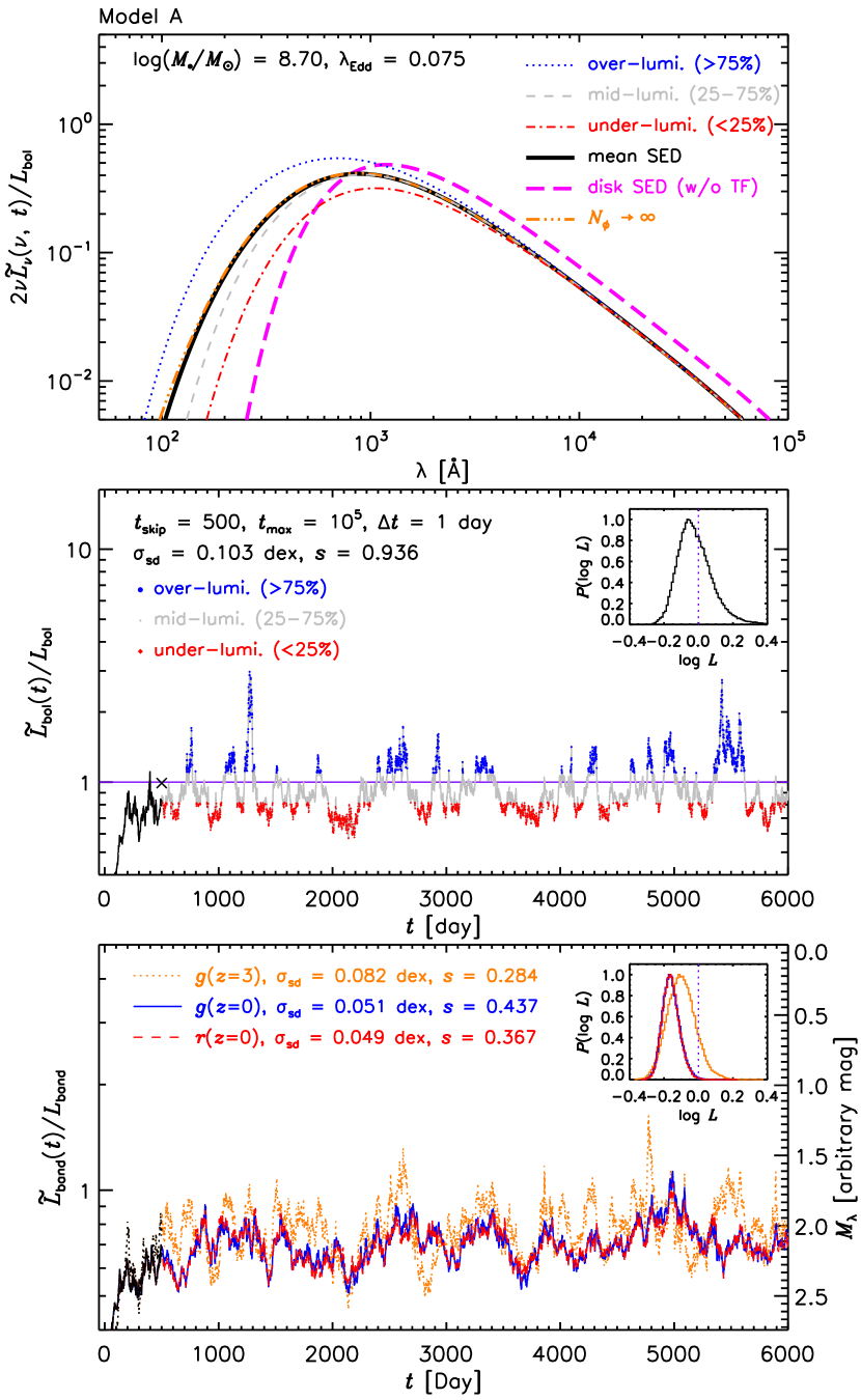
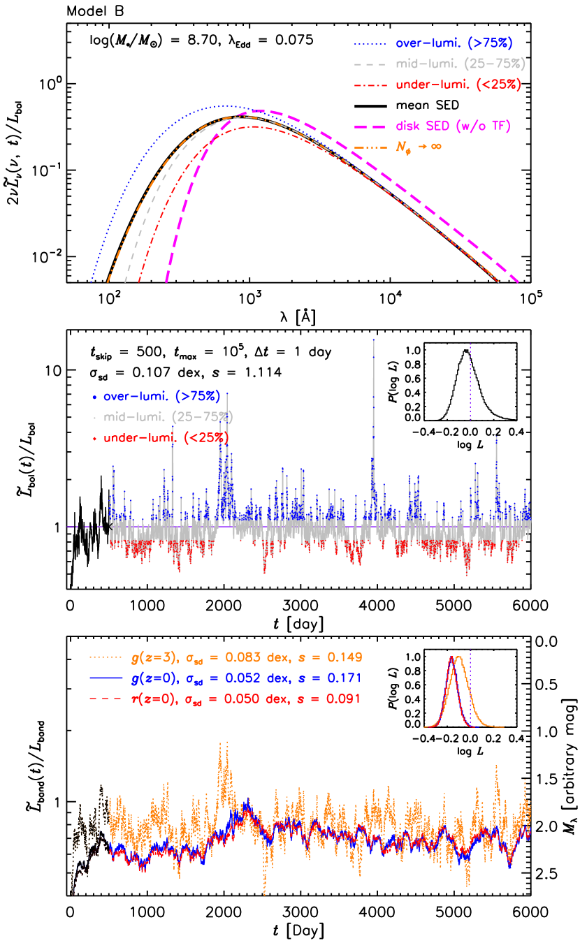
From upper to bottom panels, Figure 3 shows, respectively, an ideal example of the simulated SEDs, the light curves of the bolometric luminosity, and the light curves of the UV/optical luminosities at three different bands, for the two reference models. These light curves are ideal owing to their properties of long-enough (up to $\simeq 10^{5}$ days), no-error, and even-sampling ($\Delta t=1$ day).

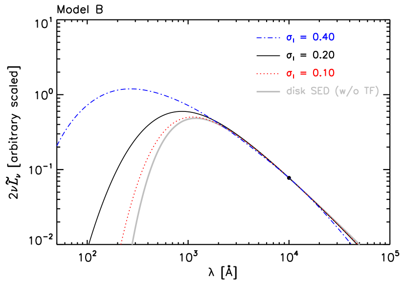
In the top panels of Figure 3, the time-averaged SEDs for both models, which are solely determined by $\sigma_{\rm l}$, appear identical to that of $N_{\phi}\rightarrow\infty$. The averaged SEDs from simulations are blued at short wavelength compared to the standard thin disk model without temperature fluctuations, and get bluer with increasing $\sigma_{\rm l}$ (cf. the bottom panel of Figure 4 and also the Figure 4 of Dexter & Agol 2011). In fact the mean SEDs averaged over different luminosity ranges, i.e., the over-luminous ($>75\%$ of luminosity distribution), mid-luminous ($25-75\%$), and the under-luminous states ($<25\%$), are almost always blued at shorter wavelength, comparing with the standard thin disk model. Meanwhile the under-luminous states ($<25\%$) could be slightly redder at $\sim$ 2000Å, particularly with larger $f_{\rm rbr}$ (thus smaller $N_{\phi}$; cf. the top panel of Figure 4). At longer wavelengths, all the simulated SEDs show little difference in the slope comparing with the thin disk model. Therefore, firstly determining the time-averaged SED would help constraining $\sigma_{\rm l}$ and then the scatter around the time-averaged SED would be able to provide further constraint on $f_{\rm rbr}$ and/or $N_{\phi}$.

In the middle panels of Figure 3, the requirement of energy conservation over time is justified by the agreement between the mean fluctuated bolometric luminosities averaged from $t_{\rm skip}$ up to $t_{\rm max}$ (black cross symbols) and those given by the standard thin disk (blue horizontal lines). The other color symbols represent the three typical epochs considered previously. Although there are rare extremely over-luminous epochs in the bolometric luminosity light curve, the radiation at these epochs exclusively concentrates at the very short wavelengths, leaving mild variations of luminosity on the other side (cf. the top panels of the same figure). The distributions of the fluctuating bolometric luminosity, $\log\tilde{L}_{\rm bol}$, are asymmetric and possesses a higher tail toward over-luminous states with skewness $s\sim 1$ for both models. Here, this skewness is estimated using the distribution constructed from 100 ideal simulations to take the scatter of skewness among simulations into account, while those nominated values in Figure 3 are solely based on that single ideal simulation. The result that the distribution of $\log\tilde{L}_{\rm bol}\sim\log\sum^{N}_{i=1}T^{4}_{i}(r,\phi)$ is not gaussian is because the distributions of $\log T_{i}$ are assumed to be gaussian but $T_{i}(r)$ spans a wide range over the whole disk (see Section 3.2 for further discussion).

The bottom panels of Figure 3 show the light curves of three UV/optical bands, $\tilde{L}_{\rm band}$, corresponding to the SDSS $r(z=0)$ (red dashed lines), $g(z=0)$ (blue solid lines), and $g(z=3)$ (orange dotted lines) bands with rest-frame effective wavelengths of $\sim 6122\,{\rm\mathring{A}}$, $\sim 4640\,{\rm\mathring{A}}$, and $\sim 1160\,{\rm\mathring{A}}$, respectively. The larger fluctuations of band luminosities at shorter effective wavelengths are intuitively illustrated and quantified by the corresponding standard deviations $\sigma_{\rm sd}$ of the fluctuating luminosities in logarithm. This result is qualitatively consistent with the observed anti-correlation between variation amplitude and wavelength. Furthermore, the other observed correlations between the UV/optical variation amplitude and the physical properties of AGNs, such as bolometric luminosity, accretion rate, BH mass, etc., can also be qualitatively argued. Particularly, for sources with smaller SMBHs and/or higher Eddington ratios, the peak of the disk SED should move toward shorter wavelength, and the resulted variation amplitude at given wavelengths longer than the peak would decrease. This would yield clear mass and/or Eddington ratio dependence of the variation amplitude at given wavelengths. However, quantitative comparison with observational data is out of the scope of this paper and will be exhaustively discussed in another upcoming paper (see Section 4.5 for further discussion).

By the way, owing to that the band luminosity at a given effective wavelength, $\lambda_{\rm eff}$, is approximately contributed by the emission from a specific narrow ring at $r_{\lambda_{\rm eff}}$ of the disk with similar $T(r_{\lambda_{\rm eff}})$, the amount of the skewness of the distributions of $\log\tilde{L}_{\rm band}$ reduces to $\sim 0.3$ for both models at those bands illustrated in the bottom panels of Figure 3, when averaging over 100 ideal simulations. We note that in Figure 3 the nominated skewness of light curves implied by model B superficially tends to be smaller by coincidence (see Section 3.2 for further discussion).

Comparing the two reference models, when their temperature fluctuation amplitudes on long timescale are identical, their overall mean SEDs are almost identical, but there would be few extraordinarily luminous epoch in the model B with radius-dependent $\tau$, due to the relatively large temperature fluctuation amplitudes on short timescales resulting from the inner regions.

3.2. Comparison with DRW

Figure 5.— The simulated bolometric, $g(z=3)$, and $r(z=0)$ band light curves (colored symbol lines from up to down; see the middle and bottom panels of Figure 3), implied by model A (top panel) and model B (bottom panel), are superimposed by the corresponding fitted ones (thin black lines), using the recipe of Kelly et al. (2009). The retrieved $\tau^{*}$ (with 1 $\sigma$ error), $\sigma^{*}_{\rm l}$, and the distributions of the standardized residuals (color symbols) of these light curves are presented with insets from left to right in the same colors. The accuracy of the fit is assessed through comparison between the distributions of the residuals (color symbols in insets) and a standard normal distribution (black curves in insets; Kelly et al. 2009).

Figure 6.— The mean simulated structure functions of bolometric, $g(z=3)$, and $r(z=0)$ band light curves (colored solid lines; see the middle and bottom panels of Figure 3 for the corresponding light curve whose structure function is one of the thin light-gray lines), implied by model A (top panel) and model B (bottom panel) through averaging over $N_{\rm sim}=10$ times of ideal simulation (thin light-gray lines), are fitted to that of a single DRW process, with $\sigma^{*}_{\rm l}$ and $\tau^{*}$ nominated in the corresponding panel (colored broken lines).

Figure 7.— The skewness distribution of 9110 Stripe 82 quasars possessing 10 or more good epochs with photometric errors in $g$- and $r$-bands $\leqslant 0.1$ mag, selected from the original sample of 9258 quasars presented by MacLeod et al. (2012). Those for 8000 simulated “real” light curves are over plotted for comparison (see Section 4.1 for their construction).

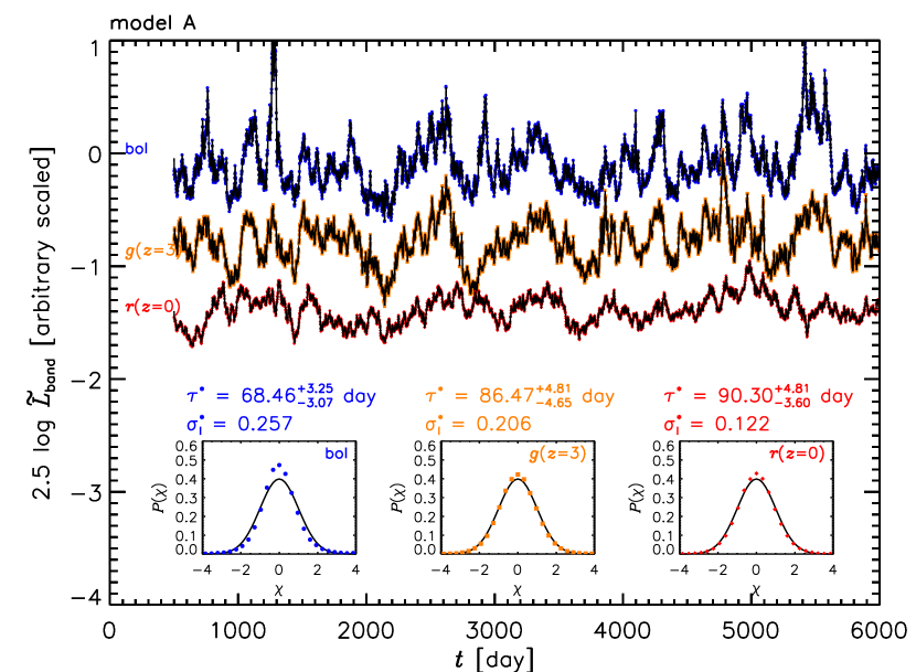
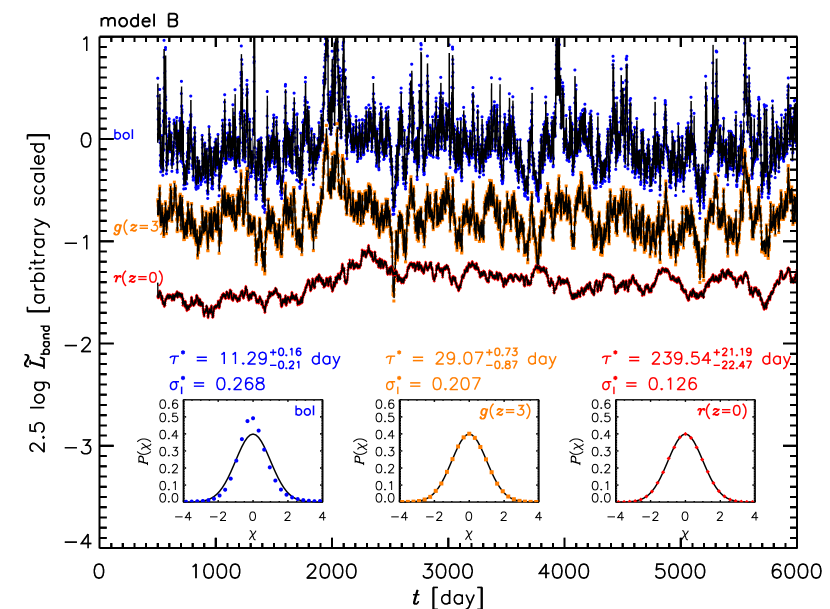
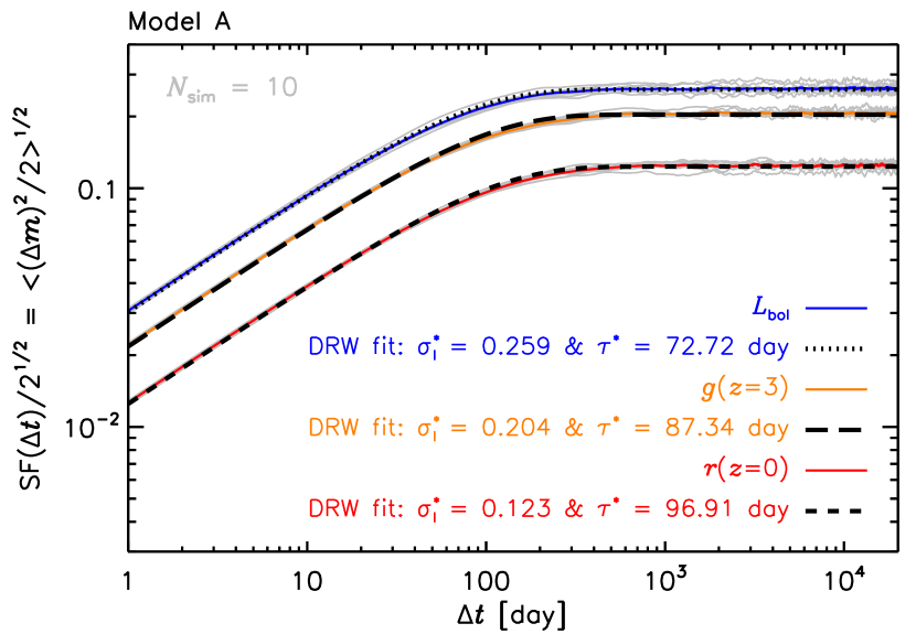
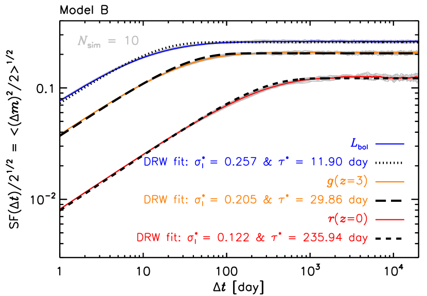
Following Dexter & Agol (2011), we have assumed $\log T$ of spatially independent zones undergoing DRW process. The thermal emission from each single disk zone therefore also follows DRW process in logarithm form ($\log L\sim 4\log T$). Although the bolometric or monochromatic emission integrated throughout the entire disk is no longer strict DRW mathematically, we show below they can be approximately modeled with DRW, by analyzing the simulated light curves (Figure 5), and the corresponding structure functions (Figure 6).

Considering the recipe of Kelly et al. (2009), we fit the simulated light curves implied by both models to retrieve the corresponding characteristic timescales, $\tau^{*}$, and the long-term fluctuation amplitudes, $\sigma^{*}_{\rm l}$ (Figure 5). For band light curves, good agreement with DRW model is reached according to the consistence between the distribution of the standardized residuals and a standard normal distribution, while for the bolometric light curves minor departures are found for both models.

Figure 6 plots the structure functions of the simulated light curves of bolometric and band (at different effective wavelength) luminosities, together with the best-fitted DRW models, i.e., $\mbox{SF}(\Delta t)=\sqrt{2}\sigma^{*}_{\rm l}\sqrt{1-\exp(-|\Delta t|/\tau^{*})}$, with long-term fluctuation amplitude, $\sigma^{*}_{\rm l}$, and the characteristic timescale, $\tau^{*}$. The structure functions are generally consistent with that of a single DRW process in shape, with only a minor departure of $\lesssim 2-4\%$ for model A and $\lesssim 4-6\%$ for model B. The slightly larger departure in shape implied in model B is attributed to the addition of fluctuations of different characteristic timescales.

We note for model A, the best DRW fits yield $\tau^{*}$ significantly smaller than the input $\tau$ for $\log T$ (200 days), and emission at shorter wavelength tends to have lower $\tau^{*}$. For the structure function of bolometric light curve, $\tau^{*}$ is even smaller owing to fact that the major contributions are dominated by the most inner regions. For model B, the difference in $\tau^{*}$ at different wavelength is more significant, due to different input $\tau$ at different disk radii, and the retrieved $\tau^{*}$ are also smaller than that of the temperature fluctuation around those radii from which the radiations dominate. For example, the characteristic timescale of the temperature fluctuation, $\sim 260$ days at $\sim 150\,r_{\rm g}$ which dominantly contribute to $r(z=0)$ band emission, is larger than the retrieved $\tau^{*}\simeq 230$ days. The difference in the characteristic timescale between the temperature fluctuations and the simulated light curves can be attributed to the complicated transformation from $\log T$ in individual disk zones to integrated luminosities. This suggests that the timescale of temperature fluctuation should be re-calibrated, instead of being simply assumed to be the same as that inferred from the observed light curves of quasars.

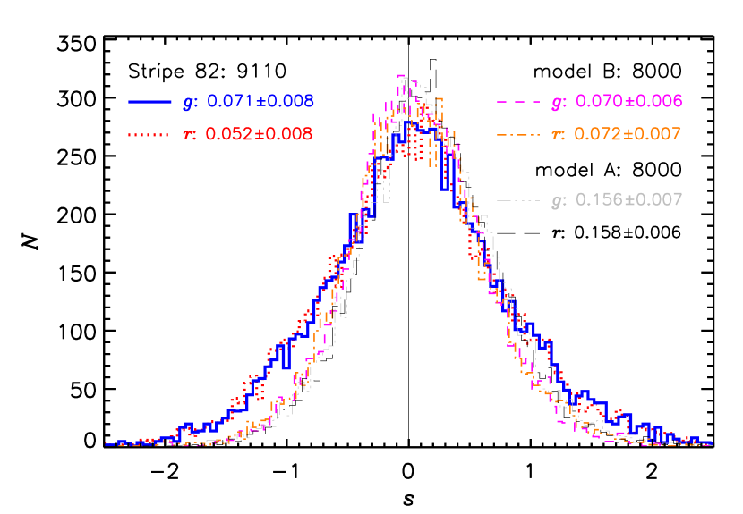
Weak deviation from DRW can also be seen through the skewness in the luminosity distributions of the simulated light curves (see Figure 3 and Section 3.1), as the luminosity distributions of perfect DRW light curves are symmetric. While the simulated ideal bolometric luminosity distributions show obvious skewness ($s$ $\sim$ 1), the skewness in the $\log L_{\rm band}$ distribution is much weaker ($s$ $\sim 0.3$ for both models).

We calculate the skewness for real $g$- and $r$-band light curves of quasars in Stripe 82, possessing 10 or more epochs with photometric errors in both bands $\leqslant 0.1$ mag (Figure 7). The observed values span a wide range for individual sources, with mean values of 0.071 and 0.052 for $g$- and $r$-bands respectively, showing weak but statistically significant positive skewness. Note the observed skewness is affected by the photometric errors and un-even sampling of SDSS Stripe 82 data. Applying the same sampling and photometric uncertainties to the simulated light curves (see Section 4.1 for details), we build a large sample of “real” $g$- and $r$-band light curves for both models and obtain the corresponding skewness (Figure 7). The simulated “real” light curves produce weaker skewness in $\log L$ distribution comparing with the ideal light curves, and the decrease of skewness is primarily due to the introduction of un-even sampling. The mean value from model B appears to be well consistent with observations (although with slightly narrow distribution), while model A yields a slightly larger value.

3.3. Bluer-when-brighter trend

Figure 8.— From top to bottom panels, shown are the arithmetic mean composite spectra, the arithmetic mean composite difference spectra, and the composite relative variability spectra, for model A (left panels) and model B (right panels), respectively. In the top panels, the composite spectra are compared to the one predicted by the standard thin disk without temperature fluctuation (red dashed line), which has been normalized to the composite one at 5000 ${\rm\mathring{A}}$ to highlight the difference at shorter wavelengths. The middle and bottom panels show the composite difference spectra and the composite relative variability spectra, constructed from pair spectra selected from the simulated ones (see Figure 3) by an interval of $\Delta t=50$ days and the total luminosity within 1300-5800 ${\rm\mathring{A}}$ changed by more than $\Delta L/L_{1300-5800{\rm\mathring{A}}}=5$% (blue dashed line), 10% (black solid line), and 20% (orange triple-dot-dashed line), respectively. The thick lines are results of averaging over $N_{\rm sim}=10$ times of ideal simulations, while results of each ideal simulation are also presented as the bundles of light-gray lines around the corresponding averaged ones. For two given wavelengths, say $\lambda_{1}<\lambda_{2}$, the bluer-when-brighter trend is indicated by the ratio of $\Delta L_{\lambda}/L_{\lambda}(\lambda_{1})$ to $\Delta L_{\lambda}/L_{\lambda}(\lambda_{2})$ larger than 1.

Figure 9.— Same as the bottom panels of Figure 8 for model A (left panel) and model B (right panel) with $\Delta t=50$ days, but for different luminosity criteria larger than 10% with broader (panchromatism; blue dashed lines) and narrower (3000-5800 ${\rm\mathring{A}}$; orange triple-dot-dashed lines) wavelength ranges to illustrate that whether or not there is a broken or bump in the composite relative variability spectrum depends on the adopted wavelength range of luminosity criterion.

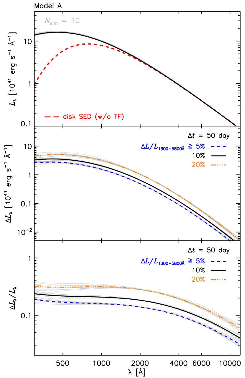
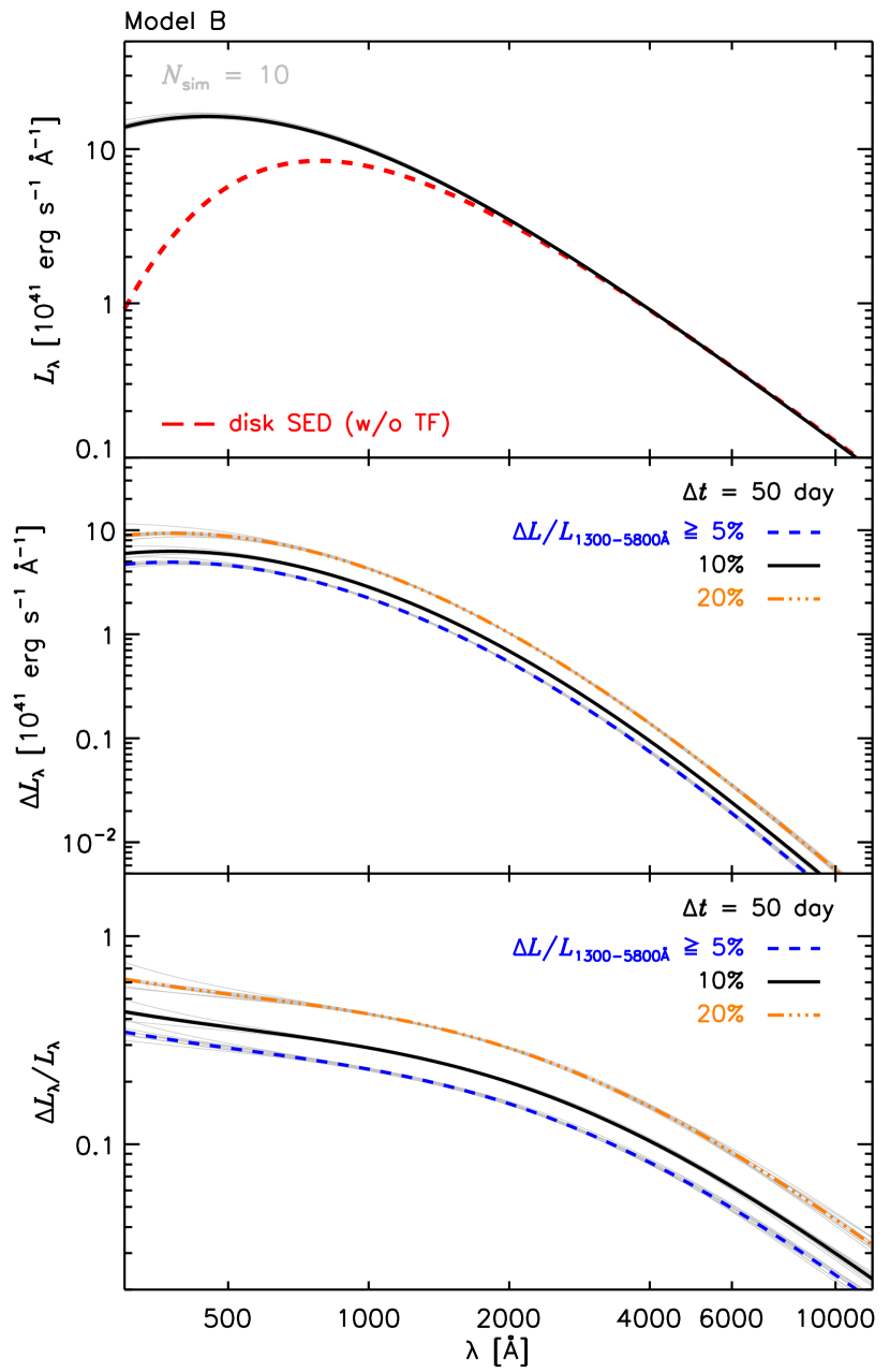
To demonstrate the well-known bluer-when-brighter trend observed in quasar variability using the ideal simulations, Figure 8 shows, from top to bottom panels, the arithmetic mean composite spectra, the arithmetic mean composite difference spectra, and the arithmetic relative variability spectra, for the two reference models, respectively. We select spectral pairs by an interval of 50 days and the total luminosity in the wavelength range of 1300-5800 ${\rm\mathring{A}}$ changed by more than 5%, 10%, and 20% from our simulated spectra (cf. Ruan et al. 2014, for the selections of time interval and wavelength range). The relative change in luminosity between $t_{1}$ and $t_{2}$ is defined as $\Delta L/L_{1300-5800{\rm\mathring{A}}}(\Delta t=|t_{1}-t_{2}|)\equiv 2|L_{1}-L_{2}|/(L_{1}+L_{2})$, where $L_{1}$ and $L_{2}$ are the integrated luminosities in the wavelength range of 1300-5800 ${\rm\mathring{A}}$ at $t_{1}$ and $t_{2}$, respectively. If $L_{2}>L_{1}$, the $t_{2}$ epoch is defined as the brighter one and the difference spectrum of the two epochs is $\Delta L_{\lambda}\equiv L_{\lambda}(t_{2})-L_{\lambda}(t_{1})$. The illustrated results are further arithmetically averaged over $N_{\rm sim}$ times of ideal simulations, while results of each ideal simulation are also presented as the bundles of light-gray lines around the corresponding averaged ones.

In the top panels of Figure 8, the composite spectra (black lines) are bluer than the spectrum predicted by the standard thin disk (red dashed line), owing to the introduction of temperature fluctuations. In the reference model B with radius-dependent $\tau$, the composite spectrum is almost identical to that implied by the reference model A with radius-independent $\tau$, because the average has been done over all epochs and the same $\sigma_{\rm l}$ has been assumed for both models.

For each model, requiring larger $\Delta L/L_{1300-5800{\rm\mathring{A}}}$ yields difference spectra with larger amplitudes, but the shapes of the difference spectra as well as the relative variability spectra, in the middle and bottom panels of Figure 8, respectively, are all analogous. The bluer-when-brighter trend is represented by the result that the relative variability continuum monotonically increases with decreasing wavelength. At short time interval, e.g., the shown $\Delta t=50$ days, model B implies bluer relative variability spectra than model A, because in model B the larger temperature fluctuations happen at inner regions than outer ones for given short time interval (e.g., 50 days). For sufficiently long time interval or when the temperature fluctuations at all radii saturate, the two models would present the same difference and relative variability spectra as long as $\sigma_{\rm l}$ is identical (see further discussion at the end of Section 4.3).

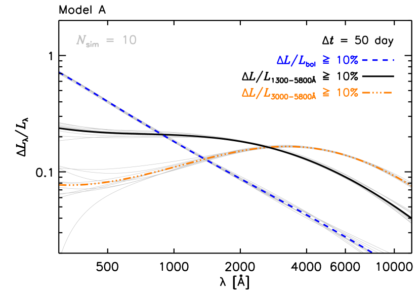
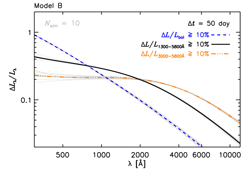
The relative variability spectra exhibit a shape of broken power-laws with characteristic broken wavelengths of $\sim$ 2000 Å. This in fact is a selection effect since these spectra are constructed requiring the luminosity in the wavelength range of 1300-5800 ${\rm\mathring{A}}$ changed by more than some percentages. Figure 9 better demonstrates such bias, in which we see that the characteristic broken wavelength in the relative variability spectrum changes after we adopt different wavelength ranges to calculate luminosity variations. The prominence of the broken, or even a bump, becomes more significant with narrower wavelength range (i.e., 3000-5800 Å), and disappears if we adopt bolometric luminosity to determine the brighter epoch. Therefore, the shapes of both the difference spectrum and the relative variability spectrum depend on the wavelength ranges adopted to determine the relative change in luminosity. One has to be cautious of such bias while comparing observed difference spectra or relative variability spectra with theoretical calculations. Note that a redder-when-brighter trend could even be observed at the bluer part of the bump if the luminosity change is determined in a narrow enough wavelength range, such as 3000-5800 Å (cf. Figure 9).

For both models, the shapes of the relative variability spectrum are broadly consistent with that presented in the explored wavelength range by Ruan et al. (2014, cf. their Figure 6), in which a narrow wavelength range 1300-5800 Å was explored using a sample of 602 variable quasars.

3.4. Timescale-dependent color variation

Figure 10.— Top panels: Amplitudes of color variation, estimated at SDSS $g$- and $r$-bands for ideal quasars at $z=0$ (black solid line), 1 (red dotted line), 2 (blue dashed line), and 3 (orange dot-dashed line), as a function of the rest-frame timescale, $\Delta t$, for the reference model A with radius-independent $\tau$ (left panel) and model B with radius-dependent $\tau$ (right panel). The shown color variations require $[(\Delta L/L_{\rm g})^{2}+(\Delta L/L_{\rm r})^{2}]^{1/2}\geqslant 10\%$, which only induces tiny timescale dependence on $\theta$ such as shown in the left panel. $\theta<45^{\circ}$ stands for a bluer-when-brighter trend and $\langle\theta\rangle$ results from averaging over $N_{\rm sim}=10$ times of ideal simulations (light-gray lines). Bottom panels: Amplitudes of color variation, estimated at SDSS $g$- and $r$-bands for three samples of simulated “real” quasars at $z=2$ with un-even sampling interval and photometric errors borrowed from the SDSS Stripe 82 data, as a function of the rest-frame timescale, $\Delta t$, for the reference model A with radius-independent $\tau$ (left panel) and model B with radius-dependent $\tau$ (right panel). One sample contains 100 sources (light-gray open squares), while the other two containing completely different 1000 sources (blue filled squares and red filled circles) are considered in order to demonstrate the possible variation between samples with the same source size. Within each $\Delta t$-bin, the averaged $\theta$ is obtained after applying the “$3\sigma$” criterion on the variation and its “$1\sigma$” error is estimated through bootstrap. For both models, regardless of real un-even sampling interval and photometric errors, the global dependence of $\langle\theta\rangle$ to timescale $\Delta t$ is guaranteed after sample averaging and is consistent with that estimated using the ideal quasars. For smaller sample size, the similar dependence still exists but with larger scatter.

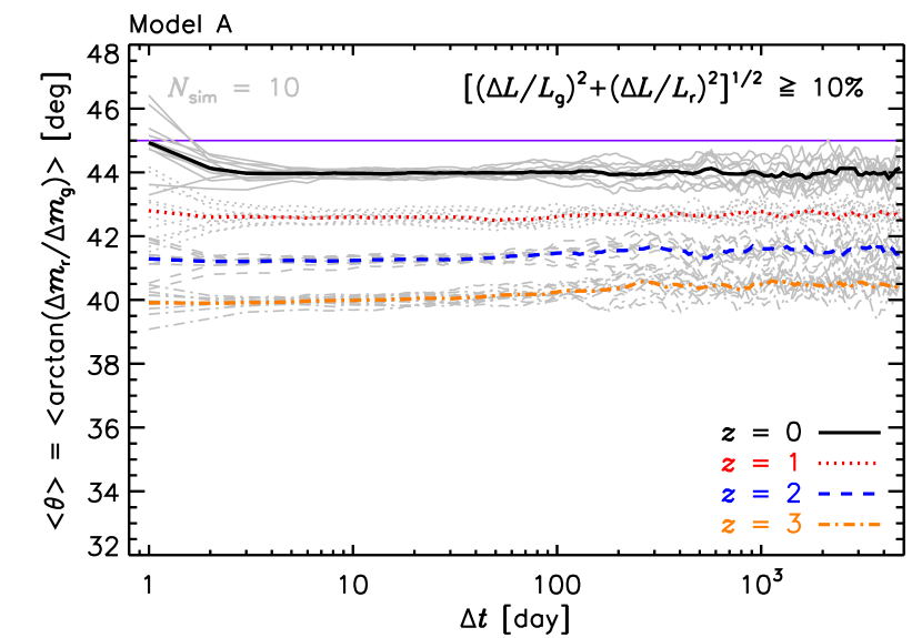
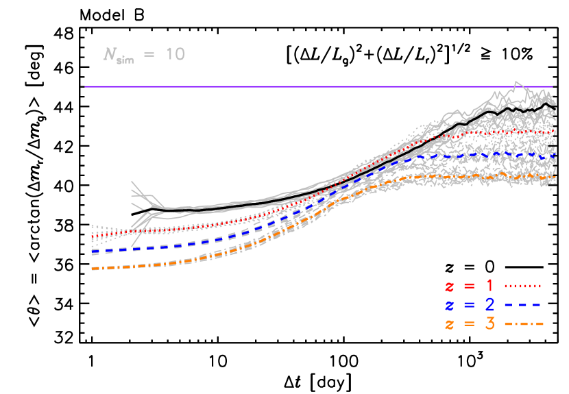
The top panels of Figure 10 shows the color variations, estimated at SDSS $g$- and $r$-bands for quasars at $z=0$ (black solid line), 1 (red dotted line), 2 (blue dashed line), and 3 (orange dot-dashed line), as a function of the rest-frame timescale for the two reference models, requiring the square root of the quadratic sum of the relative changes of successive luminosities in the two bands, i.e., $[(\Delta L/L_{\rm g})^{2}+(\Delta L/L_{\rm r})^{2}]^{1/2}$ , larger than 10%, and averaging over $N_{\rm sim}$ times of ideal simulations to reduce the fluctuations of color variation at given timescale. Following Sun et al. (2014), the amplitude of the color variation between two epochs separated by timescale $\Delta t$ is represented by a parameter $\theta$ defined as $\theta(\Delta t)\equiv\arctan(\Delta m_{\rm r}/\Delta m_{\rm g})$, where $\Delta m_{\rm g}$ and $\Delta m_{\rm r}$ are the differences of apparent magnitudes between successive epochs separated by $\Delta t$ in $g$- and $r$-bands, respectively. Accordingly, $\theta<45^{\circ}$ and $\theta>45^{\circ}$ stand for bluer-when-brighter and redder-when-brighter, respectively.

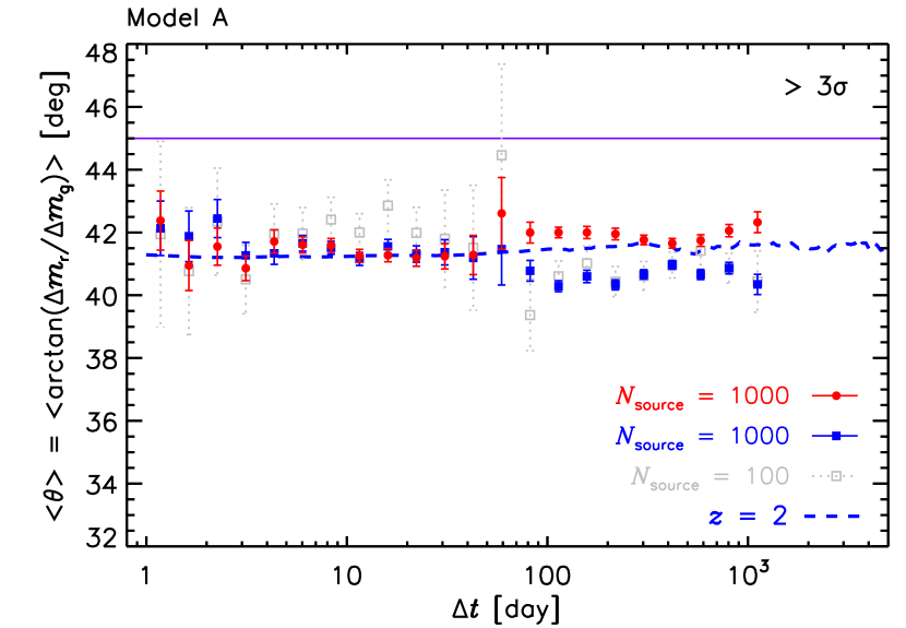
For the reference model A with radius-independent $\tau$, the averaged $\theta$ over all epoch pairs separated by the timescale $\Delta t$ does not exhibit statistically significant dependence on $\Delta t$ as expected (see the top-left panel of Figure 10). The tiny timescale dependence results from the requirement of $[(\Delta L/L_{\rm g})^{2}+(\Delta L/L_{\rm r})^{2}]^{1/2}\geqslant 10\%$, because the relative change of luminosity at shorter wavelength, e.g., $\Delta L/L_{\rm g}$, is generally larger than that at longer one, e.g., $\Delta L/L_{\rm r}$, and therefore the smaller $\theta$ is preferred under the requirement, especially at shorter timescales. In short, considering this kind reference models with radius-independent $\tau$, there is no significant timescale dependent color variations and they are hard to explain the timescale dependent color variations of quasars recently discovered by Sun et al. (2014).

For given observed wavelength pair, model A, as well as model B, imply smaller $\theta$ with increasing the source redshift (see the upper panels of Figure 10). Interesting, Figure 4 of Schmidt et al. (2012) may have presented a similar trend, where Schmidt et al. demonstrated that the observed color variance of Stripe 82 quasars is strongly redshift-dependent. They show such redshift dependence can be largely contributed to contaminations from the broad emission lines which do not respond to the continuum variations. Nevertheless, in their Figure 4 we can still see the observed color variation more prominent than their model at $z>1$, while at $z<1$ the model and the observed values are generally consistent. This may hint that the observed intrinsic color variation of continuum is stronger at higher redshift (i.e., smaller Schmidt et al.’s $s_{\rm gr}$ or our $\theta$), similar to the pattern shown in the upper panels of our Figure 10. However, cautions should be kept in mind that both the neglected reverberation time delays between the continuum and the lines in the simple spectral variability model of Schmidt et al. (2012) and the likely significant contributions of the variability of Balmer continuum from the broad line region in the quasar near-UV spectra (e.g., Edelson et al. 2015) may all be responsible for the discrepancy between the observed redshift dependence of color variability and the simulated one by Schmidt et al. (2012).

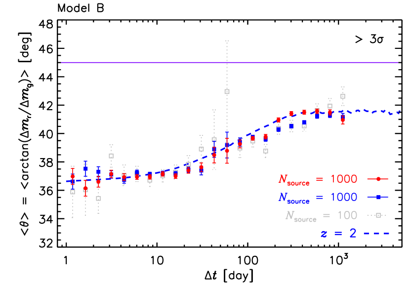
Obviously, the reference model B with radius-dependent $\tau$ (the top-right panel of Figure 10) possesses qualitatively similar timescale dependent color variations as found by Sun et al. (2014). Moreover, we see that the expected dependence of $\langle\theta\rangle$ to timescale $\Delta t$ is more prominent at intermediate timescales, and is obviously weaker toward much shorter or longer timescales.

4. Discussion

4.1. Constructing simulated “real” sample

Figure 11.— An illustration for constructing the simulated “real” light curves. The top panel shows the probability distribution of sampling in the observed frame with a time bin of one day, constructed using all the Stripe 82 sources considered by Sun et al. (2014) and the first observing epoch of each source is shifted to be the same. The middle and bottom panels show examples of the simulated “real” $g$- (blue points) and $r$-band (red points) light curves, by convolving the probability distribution of sampling with the corresponding ideal light curves (light-gray points, in steps of one day in the observed frame).

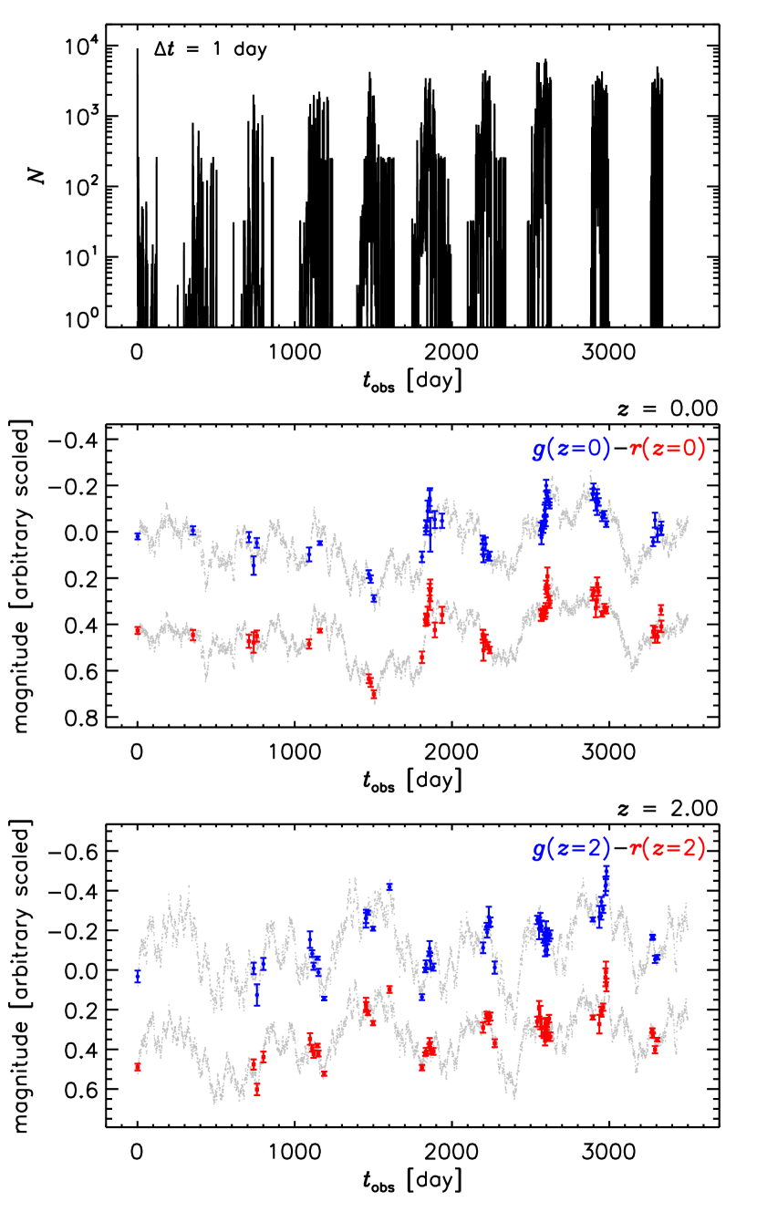
Although a qualitatively similar timescale dependent color variation as found by Sun et al. (2014) has been discussed using the ideal light curves implied by model B in the previous section, some other observational facts, such as photometric errors and un-even sampling (e.g., Palanque-Delabrouille et al. 2011, for SDSS photometries), should be properly taken into account before the delicate comparison with real data can be made and to assess their effects on the measured $\langle\theta\rangle$ – $\Delta t$ relation.

To be compared with the data by Sun et al. (2014), we use all the sources considered by Sun et al. (2014) to get the $\langle\theta\rangle$ – $\Delta t$ relation averaged over all redshifts, to derive a probability distribution of sampling in the observed frame with a time bin of one day (cf. the top panel of Figure 11). For a source at redshift $z$ observed at SDSS $g$- and $r$-bands, we first simulate the ideal $g(z)$ and $r(z)$ light curves in steps of one day in the observed frame, which are randomly convolved with the probability distribution of sampling. Random photometric uncertainties are added to every pair of both light curves of each simulated source, with a pair of photometric errors of $g$- and $r$-bands taken randomly from real quasars in the same redshift bin, and furthermore, Gaussian deviates with zero mean and standard deviation equal to the randomly selected photometric uncertainty of each point are added to mimic the measurement errors (cf. the middle and bottom panels of Figure 11 for examples of $g$- and $r$-band light curves of sources at $z=0$ and 2, respectively). We consider the same redshift bins as explored by Sun et al. (2014) in order to compare the $\langle\theta\rangle$ – $\Delta t$ relation averaged over quasars within different redshift bins. This sample of $N$ sources at redshift $z$ is then used to calculate the $\langle\theta\rangle$ – $\Delta t$ relation at $z$ after applying the “$3\sigma$” criterion on the variation as done by Sun et al. (2014), and bootstrapped to estimate its “$1\sigma$” errors.

In the bottom panels of Figure 10 , we show that the simulated “real” light curves, after applying photometric errors and un-even sampling borrowed from the SDSS Stripe 82 data and the “$3\sigma$” criterion on the variation, yield $\langle\theta\rangle$ – $\Delta t$ relations well consistent with those from the ideal light curves. This also demonstrates that the observed timescale dependent color variation by Sun et al. (2014) can not be attributed to such observational effects.

4.2. Dependence on model parameters

Figure 12.— Amplitudes of color variation, estimated at SDSS $g$- and $r$-bands for a sample of 1000 simulated “real” quasars at $z=2$ (symbols) with un-even sampling interval and photometric errors borrowed from the SDSS Stripe 82 data, as a function of the rest-frame timescale, $\Delta t$, implied by model A (left panels) and model B (right panels) with different parameters. The adjusted parameters for both models are the BH mass, $M_{\bullet}$, the Eddington ratio, $\lambda_{\rm Edd}$, the long-term temperature fluctuation amplitude, $\sigma_{\rm l}$, and the radial boundary ratio of split zones, $f_{\rm rbr}$, respectively, compared to the reference model with $M_{\bullet}=5\times 10^{8}\,M_{\odot}$, $\lambda_{\rm Edd}=0.075$, $\sigma_{\rm l}=0.2$, and $f_{\rm rbr}=1.3$ (black filled circles). The lines, indicating the relations implied by the corresponding 1000 simulated “real” quasars with photometric errors borrowed from the SDSS Stripe 82 data but with even sampling of one day in the observed frame, are shown in order to better demonstrate the dependence of the relation on these parameters.

Figure 13.— Same as Figure 12, except that the adjusted parameters are two unique ones of model B, i.e., $\tau_{0}$ (left panel) and $\alpha$ (right panel).

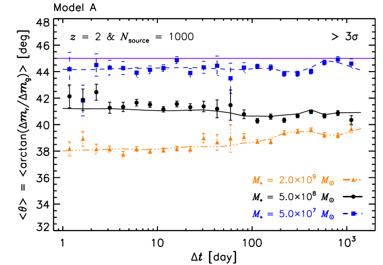
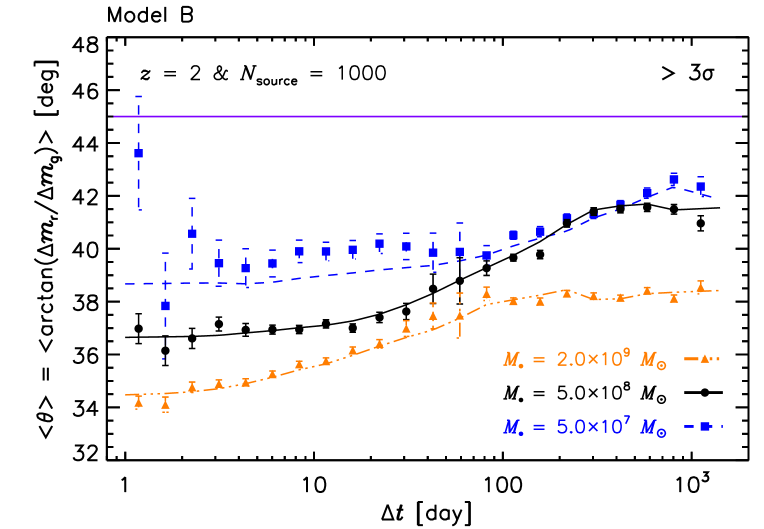
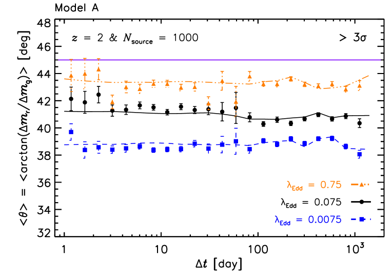
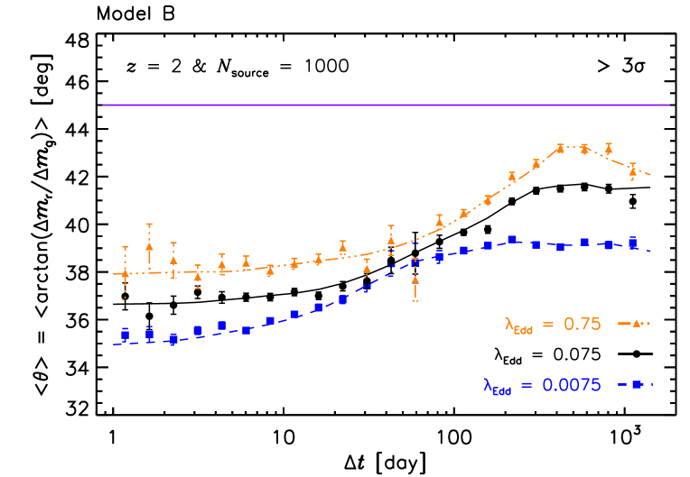
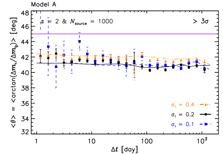
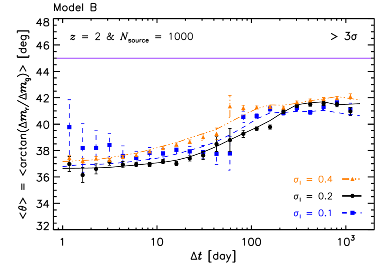
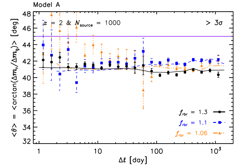
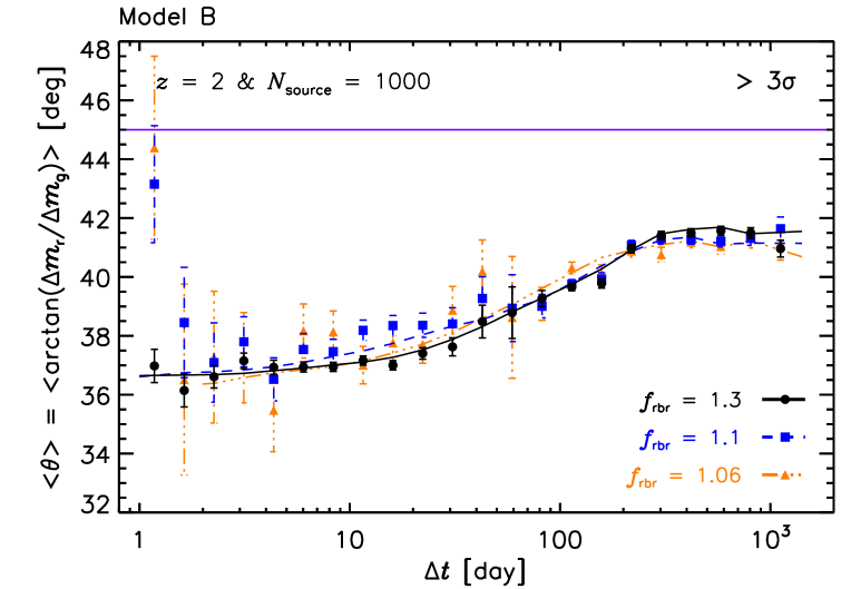
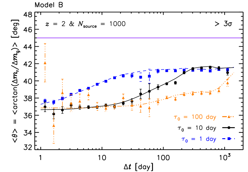
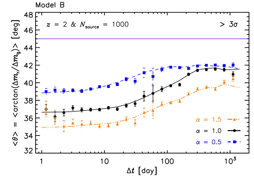
Up to now, we have mainly focused on the reference models with a single set of fixed parameters. Instead, Dexter & Agol (2011) and Ruan et al. (2014) have explored a range of parameter space (i.e., the number of fluctuating zones per factor of two in radius, $n\simeq 300-1000$, the amplitude of long-term temperature fluctuation, $\sigma_{\rm T}\simeq 0.35-0.5$, the Eddington ratio, $\lambda_{\rm Edd}\simeq 0.07-0.16$, and the BH mass, $M_{\bullet}\simeq 3\times 10^{8}-3\times 10^{9}~{}M_{\odot}$) for the inhomogeneous disk model (analog to model A) to explain observations, including the disk size measurements, the optical variability amplitudes, the UV spectral slope, and the composite different spectrum of quasars.

In Figure 12 we explore the impacts of changes of these parameters on the $\langle\theta\rangle$ – $\Delta t$ relation (symbols), estimated at SDSS $g$- and $r$-bands for a sample of 1000 simulated “real” quasars at $z=2$ with un-even sampling interval and photometric errors borrowed from the SDSS Stripe 82 data, implied by both models. To better demonstrate the dependence of the relation on these parameters, the relations (lines) implied by the corresponding 1000 simulated “real” quasars with photometric errors borrowed from the SDSS Stripe 82 data but with even sampling of one day in the observed frame are illustrated as well.

From upper to bottom panels of Figure 12, shown are the results by changing $M_{\bullet}=5\times 10^{7}-2\times 10^{9}~{}M_{\odot}$, $\lambda_{\rm Edd}=0.0075-0.75$, $\sigma_{\rm l}=0.1-0.4$ (equivalent to $\sigma_{\rm T}=0.14-0.56$), and $f_{\rm rbr}=1.06-1.3$ (equivalent to $n=1284-64$), respectively. For both models, the effects of changing these parameters on the $\langle\theta\rangle$ – $\Delta t$ relation are qualitatively similar. Note that quasars at higher redshift generally possess smaller $\langle\theta\rangle$, estimated at SDSS $g$- and $r$-bands for all timescales, or at the shorter wavelength pair the smaller $\langle\theta\rangle$ (cf. Figure 10). Considering the $\langle\theta\rangle$ estimated at the same two bands for quasars with the same redshift but different other parameters as illustrated in Figure 12, it becomes larger with decreasing $M_{\bullet}$ or increasing $\dot{M}$ (or $\lambda_{\rm Edd}$ for a fixed BH mass). The dependence on $M_{\bullet}$ or $\dot{M}$ can be understood as follows. The lower $M_{\bullet}$ or higher $\dot{M}$ the hotter the disk at given radius, the emissions contributing to the $g$- and $r$-bands come from relatively outer radii, i.e., equivalent to longer wavelength pair, and therefore, larger $\langle\theta\rangle$. Meanwhile, for model B, the outer radii correspond to longer characteristic timescales of temperature fluctuation and, consequently, the saturation of $\langle\theta\rangle$ happens at longer timescales. Considering the dependence on $\sigma_{\rm l}$, since larger $\sigma_{\rm l}$ induces hotter mean SED (cf. the bottom panel of Figure 4) and equivalent emissions come from outer radii, the $\langle\theta\rangle$ becomes larger with increasing $\sigma_{\rm l}$. Finally, no dependence on $f_{\rm rbr}$ is found for both models. This suggests that the $\langle\theta\rangle$ – $\Delta t$ relation can not provide any constraint on the number of fluctuating zones.

Comparing with model A, model B introduces two extra parameters, i.e., the minimal timescale at the inner most radius, $\tau_{0}$, and the index of radius dependence, $\alpha$. The effect of $\tau_{0}$ on the relation is simply shifting the $\langle\theta\rangle$ – $\Delta t$ plot horizontally (cf. the left panel of Figure 13). The impact of changing $\alpha$ is however more complicated. While it is expected that smaller $\alpha$ (e.g., 0.5) produces weaker correlation between $\langle\theta\rangle$ and $\Delta t$, a larger $\alpha$ (e.g., 1.5) does not give a steeper slope comparing with $\alpha$ = 1.0 (cf. the right panel of Figure 13). Referring to explanations in last two paragraphs of Section 4.3, larger $\alpha$, which produces relatively stronger inner disk fluctuations comparing with outer disk at short timescales, yields bluer variable emission thus smaller $\langle\theta\rangle$ at small $\Delta t$. With increasing $\Delta t$, $\langle\theta\rangle$ starts to gradually increases to a saturation point when both inner and outer disk fluctuations do not grow anymore. While the value of saturated $\langle\theta\rangle$ is independent to $\alpha$, the saturation point moves to longer timescale for larger $\alpha$, thus further increasing $\alpha$ does not significantly alter the $\langle\theta\rangle$ – $\Delta t$ slope.

4.3. Comparison to the Stripe 82 data

Figure 14.— Amplitudes of color variation of Stripe 82 quasars (blue solid line plus filled circles for the considered redshift bins; pink dotted line for narrower redshift bins) and of model B (orange dashed line plus filled squares, inferred from the orange dashed lines in Figure 15), averaged over rest-frame $10^{2}<\Delta t<10^{3}$ days. The amplitude difference between blue filled circle and orange filled square is attributed to emission line contributions and adopted as the empirical factor for correction at each redshift.

Figure 15.— Comparison between the color variations of Stripe 82 quasars in different redshift bins (blue filled circles, Sun et al. 2014) and those implied by the model B with $\tau_{0}=10~{}(M_{\bullet}/10^{8.75}M_{\odot})$ days and $\alpha=1$, empirically corrected for emission line contributions (thick black lines; see also Figure 14). The model predictions prior to corrections are also plotted (orange dashed lines). The adopted model parameters are indicated at the lower-left corner of each panel. In each redshift bin, the adopted typical redshift is chosen close to the mean/median of the subsample of Stripe 82 quasars, while the adopted typical BH mass and Eddington ratio are respectively the peaks of BH mass and Eddington ratio distributions for those quasars with both BH mass and Eddington ratio measurements (small blue dots in the inserted plot, with the range of the redshift bin at the lower-left corner and the number ratio of quasars with both BH mass and Eddington ratio measurements to all sources in the bin at the upper-right corner; Shen et al. 2011). For comparisons, the similarly corrected relations implied by model A (light-gray thin triple-dot-dashed lines) and by model B but with $\alpha=1.5$ (red thin solid lines) are also shown.

As demonstrated in the previous sections, the timescale independent color variations implied by model A, similar to that of Dexter & Agol (2011), with radius-independent $\tau$ for temperature fluctuations conflict with the discovery of a timescale dependent color variations by Sun et al. (2014). Neither the selection of model parameters nor the observational defects, e.g., un-even sampling and/or photometric error, can alleviate the tension. Therefore, later on, we will mainly compare the predictions implied by model B with observations of Sun et al. (2014).

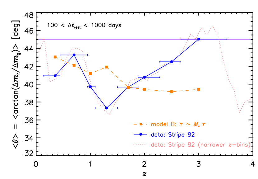
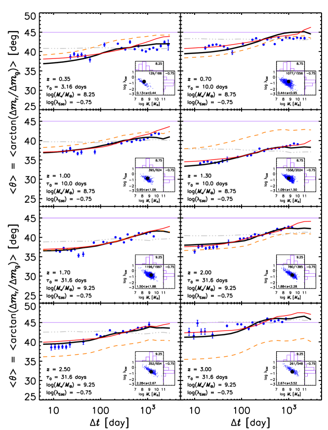
Since only the continuum emission of the accretion disk is considered in the current model, one needs to correct for emission line contributions on the $\langle\theta\rangle$ at different redshift bins. Schmidt et al. (2012) have shown the redshift dependence of the color variation amplitude of SDSS quasars (up to $z\sim 3$) is more consistent with the assumption that the emission lines in quasar spectra simply do not follow the continuum variation (cf. their Figure 4). Consequently, we estimate the $\langle\theta\rangle$ averaged over rest-frame $10^{2}<\Delta t<10^{3}$ days for both Stripe 82 quasars and simulated “real” quasars in model B with $\tau_{0}=10~{}(M_{\bullet}/10^{8.75}M_{\odot})$ days and $\alpha=1$, in several redshift bins as illustrated in Figure 14, and attribute their differences to the contaminations of emission lines to certain bands. The model predicted $\langle\theta\rangle$ – $\Delta t$ relation can then be empirically corrected for direct comparison with observations (Figure 15). Note that this procedure is somewhat arbitrary (see Section 4.5 for further discussion). The same procedure has been applied for model A to illustrate the completely different $\langle\theta\rangle$ – $\Delta t$ relation. Within each redshift bin, the model predictions are inferred with the typical values of redshift, $\tau_{0}$, BH mass, and Eddington ratio, nominated at the lower-left corner of each panel (see the legend of Figure 15 for the selection of these typical values).

After correction, the general consistence between the shapes of the $\langle\theta\rangle$ – $\Delta t$ relation implied by Stripe 82 quasars (blue filled circles) and by model B with $\tau_{0}=10~{}(M_{\bullet}/10^{8.75}M_{\odot})$ days and $\alpha=1$ (black thick solid lines in Figure 15) is encouraging, in consideration of the simplicity/caveats of the current model. In the two lowest redshift bins, the observed $\langle\theta\rangle$ – $\Delta t$ slopes however appear slightly flatter than the model prediction. One possibility is that X-ray reprocessing (e.g., Krolik et al. 1991) in quasars with lower luminosities, in which the X-ray to bolometric luminosity ratio is higher, could contribute more to optical/UV variation, and its color variation dependence to timescale could be different from thermal fluctuation in the disk. We will leave this issue to a future dedicated study.

Moreover, we also plot in Figure 15 the model prediction with $\alpha$ = 1.5, the agreement between which and the observation is also remarkable, but not as good as $\alpha$ = 1.0. Considering the model predicted slopes in $\langle\theta\rangle$ – $\Delta t$ rely on various parameters which we can not well constrain (see Figures 12 and 13), it is immature to conclude that which $\alpha$ is more favored by observations, and we are yet unable to pin down $\alpha$ and therefore possible physical mechanism responsible for the temperature fluctuations delineated by some characteristic timescales, e.g., the viscous timescale of $\tau\sim r^{5/4}$ (Alloin et al. 1985) or the thermal (cooling) timescale of $\tau\sim r^{3/2}$ (Collier & Peterson 2001; see also Lawrence 2012).

Figure 16.— The arithmetic mean composite difference spectra for model A (left panel) and model B (right panel), requiring $[(\Delta L/L_{\rm g})^{2}+(\Delta L/L_{\rm r})^{2}]^{1/2}\geqslant 10\%$ at different $\Delta t=5$ (blue dashed line), 50 (blue solid line), 500 (blue triple-dot-dashed line), and 5000 days (light-gray long-dashed line), and averaging over $N_{\rm sim}=10$ times of ideal simulations. The similar difference spectra at different timescales implies that the color variation is timescale independent, such as those given by model A. In model B with radius-dependent $\tau$, the difference spectrum is prominent timescale dependent, i.e., bluer at shorter timescales. At long timescales, both models present the same difference spectra as illustrated by the agreement between the light-gray thin solid line implied by model A and that by model B at $\Delta t=5000$ days in the right panel. For simplicity the plotted wavelength range has been limited to be close to $g$- and $r$-bands, to alleviate suffering from the same selection effect as shown in Figure 9.

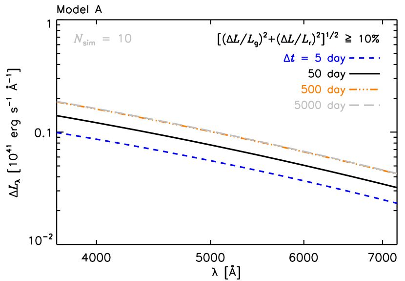
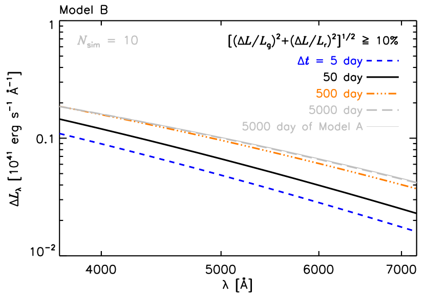
The timescale dependence of the color variation in Figures 10, 12-13, and 15 implied by model B can be interpreted as follows. At given wavelength, the radiation mainly comes from a certain range of disk radius. At very short timescales, the fluctuations at inner disk are stronger comparing with those at outer disk, thus the produced variation emission is rather blue (with $\langle\theta\rangle$ significantly smaller than $45^{\circ}$). The fluctuations in disk zones at smaller radii (such as those contribute significantly to $g$-band emission) and at larger radii (such as those contribute to $r$-band emission) both gradually increase towards larger timescales. This yields larger amplitude in flux variation in both $g$- and $r$-bands with increasing timescale, but the color of the variation remains constant. Therefore $\langle\theta\rangle$ appears insensitive to $\Delta t$, e.g., in the top-right panel of Figure 10 at small $\Delta t$. At intermediate timescales, however, the fluctuations in disk zones at smaller radii begin to saturate, while the fluctuations at larger radii still steadily increase. Disk emission at larger radii which is redder thus makes relatively stronger contribution to the output flux variation with increasing timescales, and increases $\langle\theta\rangle$ accordingly. At even larger $\Delta t$, the fluctuations in the outer disk zones also saturate, thus the color of the variation is again timescale independent. An interesting consequence is that for a single AGN one may not be able to detect the timescale dependency of the color variation at certain ranges of timescales.

There is an intimate connection between the color variations and the mean difference spectra at different timescales. The similar shapes of difference spectra at different timescales would imply color variations are timescale independent, such as those given by model A (the left panel of Figure 16). However, for model B with radius-dependent $\tau$, the difference spectrum is prominent timescale dependent, that is, it is steeper and corresponds to more significant bluer-when-brighter at shorter timescale. Instead, at very long timescales, both models present the same difference spectra as well as the averaged $\theta$, as at long enough timescales, the fluctuations of the inner and outer disk zones all saturate at the same amplitude for both models.

4.4. An artifact or not?

Using the $B$- and $V$-band monitoring on 3C 120, Ramolla et al. (2015) did not find strong timescale dependence in its color variability, analyzed in flux-flux space on two ranges of timescales, i.e., 0-120 days and 1600-2000 days. They proposed that the reported timescale dependence of the color variability by Sun et al. (2014) is likely an artifact caused by analyzing the data in magnitude space. Considering the host galaxy contamination (stronger in redder band) would reduce the variation amplitude in magnitude space, Ramolla et al. (2015) argued that, at longer timescales, as the flux variation amplitude is larger, the host contamination is reduced, and therefore, the color variation measured in mag-mag space appears weaker.

However, the host galaxy contamination (in magnitude space) only depends on the brightness of the nucleus at given epoch, but not the time lags between epochs. In other words, photometric data points with longer time lags between epochs although tend to have larger flux differences, these epochs do not correspond to brighter states on average in the nucleus emission. Therefore, the logic that the host contamination is weaker at longer timescales is incorrect, and analyzing the color variation in mag-mag space would not produce an artificial timescale dependence.

In fact, analyzing the Stripe 82 quasars in flux-flux space also produces clear timescale dependent color variation pattern, in agreement with the results in mag-mag space (see also discussions in Section 4.5). Monte Carlo simulations also confirm that host galaxy contamination does not produce artificial timescale dependence in the color variation. Furthermore, using the same data of 3C 120 from Ramolla et al. (2015), the timescale dependence in its color variation is found to be consistently weak in both mag-mag and flux-flux spaces. The absence of strong timescale dependence in the color variation in 3C 120 is likely due to 1) the light curve is not long enough to reveal the signal; 2) for AGNs with lower luminosities like 3C 120, X-ray reprocessing would be dominant and can yield timescale independent color variation (at timescales longer than the light travel time from corona to the corresponding disk radii); 3) 3C 120 contains a smaller SMBH with mass $\simeq 5\times 10^{7}~{}M_{\odot}$ (Nelson 2000; Peterson 2014) than quasars, thus the timescale dependence can only be detected at much shorter timescales (see the left panel of Figure 13 for instance); or 4) radio loud AGNs behave differently. Details on these issues will be presented in an upcoming paper (Sun et al. in prep).

4.5. Caveats

Sun et al. (2014) discussed that neither the contamination from the host galaxy nor the changes of the global accretion rate can address the timescale dependent color variation. They suggested that shorter term variations could be attributed to thermal fluctuations in the inner region of the accretion disk, while longer term variations to larger scales. We examine this explanation by simply considering another revised reference model B with radius-dependent $\tau$ for temperature fluctuations, which is in fact a natural assumption as the physical size of the disk cells is proportional to the radius. By doing so we achieve qualitatively similar timescale dependent color variations, as illustrated in the right panels of Figure 10, and further quantitative trends in shape, as illustrated in Figure 15, after empirically correcting for emission line contributions. We note that this revised reference model would also imply consistent microlensing disk sizes as in the original Dexter & Agol model since the time-averaged disk half-light radius is primarily determined by the long-term amplitude of temperature variance, $\sigma_{\rm l}$ or $\sigma_{\rm T}$ (see Equation 4 of Dexter & Agol 2011).

However, the contributions of emission lines to the broadband photometry at various redshifts have only been empirically taken in account in the present model (see Section 4.3). In principle, what is compared between observations and simulations in this work is the slope of $\langle\theta\rangle$ – $\Delta t$ relation from simulations with observations, but not the absolute values of $\langle\theta\rangle$ (or the absolute amplitude of color variation). As broadband photometry is affected by not only the accretion disk continuum emission, but also the broad/narrow emission lines, the Balmer continuum (e.g., Kokubo et al. 2014; Edelson et al. 2015), and the host galaxy emission, recovering the absolute value of $\theta$ and its dependence to redshift through simulations is not straightforward and beyond the scope of this work. Schmidt et al. (2012) have tried to construct a simple spectral variability model, including a single power-law (with variable slope and a pivot point in the IR) and an emission line template, to reproduce the observed color variability redshift dependence. However a single power-law, as assumed by Schmidt et al. (2012), may be not a good enough description of real quasar spectrum when extending to UV wavelengths, and therefore, may bias the estimated color variation amplitudes (i.e., Schmidt et al.’s $s_{\rm gr}$ or our $\theta$), especially at high redshifts. Furthermore, it is oversimplified to assume all quasars have the same emission line template spectrum, and these lines correspond or do not correspond to the continuum variation uniformly without lags. These factors may in fact be responsible for the discrepancy between the observed redshift dependence of color variation and the one simulated by Schmidt et al. (2012, see their Figure 4).

Figure 17.— Same as Figure 15, except that the $\theta$ is estimated in flux-flux space, rather than mag-mag space. The data points (blue circles) are re-derived in flux-flux space as well using the same sources with bootstrapping errors. The results implied by the model B with $\tau_{0}=10~{}(M_{\bullet}/10^{8.75}M_{\odot})$ days and $\alpha=1$, empirically corrected for emission line contributions, are illustrated as the thick black lines. The model predictions prior to corrections are also plotted (orange dashed lines). The adopted model parameters are indicated at the lower-right corner of each panel. For comparisons, the similarly corrected relations implied by model A (light-gray thin triple-dot-dashed lines) and by model B but with $\alpha=1.5$ (red thin solid lines) are also shown.

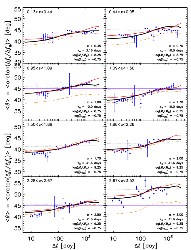
Alternatively, the analyses can be performed in flux-flux space to directly measure the color of difference spectrum, which is free from contamination of non-variable component. However, as shown in Kokubo et al. (2014), the color of difference spectrum of quasars shows also clear redshift dependence due to variable emission lines and Balmer continuum, indicating the effects of which can not be neglected either for analyses in flux-flux space. In Figure 17 we present plots similar to Figure 15, but with $\theta$ measured in flux-flux space, instead of in mag-mag space. As expected, arbitrary shifts are still required to match the absolute values of $\theta$ from simulations to observations. Nevertheless, the slope in the $\theta$ – $\tau$ relation is again nicely reproduced by our simulations.

The parameters of the inhomogeneous disk ($\tau$, $\sigma_{\rm l}$ and their possible radius dependence) could also depend on SMBH mass and accretion rate, for which the observed sample span considerably large ranges, instead of the single values we adopted in this work. More fundamentally, the inhomogeneous disk model still encounters two problems. One of them is that the thin accretion model predicts bluer UV spectra than observed (see review by Lawrence 2012). Once introducing temperature fluctuations, the time-averaged SED is even bluer than the one without (see the top panels of Figures 3 or 8). Therefore, the tension between the observed composite SED and the modeled one predicted by the thin disk would be further aggravated. On the other hand, dust extinction and/or disk outflow could yield redder disk SEDs (e.g., Capellupo et al. 2015).

Nevertheless it is complicated by the extensive debate on whether the origin of AGN SED can be attributed to a geometrically thin, optically thick accretion disk or not (see reviews by Koratkar & Blaes 1999; Davis & Laor 2011). To finally settle down the delicate dependence of $\tau$ and $\sigma_{\rm l}$ on radius for inhomogeneous disk model, we need to firstly work on a more realistic disk model. It is possible as demonstrated by Capellupo et al. (2015) that the thin accretion disks are indeed, if not all, responsible for the origin of AGN SEDs once included various improvements, such as general relativistic corrections, radiation transfer in the disc atmosphere, dust extinction, and/or disk winds (e.g., Hubeny et al. 2001; Davis & Laor 2011; Slone & Netzer 2012).

Figure 18.— Cross-correlation functions between simulated light curves at different wavelengths (labelled with SDSS $g$- and $r$-band at different redshifts) implied by model A (light-gray thin lines) and model B (colored thick lines). For both models, the correlations between $g$- and $r$-bands at all redshifts are strong and almost the same at zero lag, except that when the wavelength difference is larger, e.g., $g(z=3)$-$r(z=0)$. The widths in the cross-correlation functions reflect the characteristic timescales in the variation in corresponding light curves.

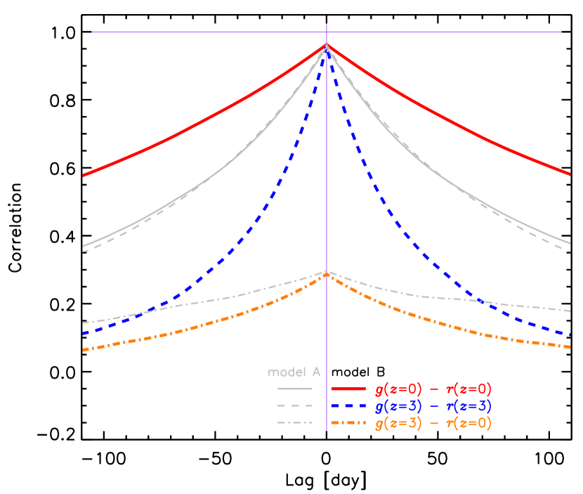
The second one is the so-called coordination problem. Observationally, the variations of several Seyfert galaxies and few quasar at different UV/optical wavelengths are found to be quite coordinate (Krolik et al. 1991; see review by Lawrence 2012 and references therein). Delicately comparing the simulated inter-band correlations with observed ones are useful to testify and further improve the inhomogeneous disk models. The bottom panel of Figure 3 shows the simulated light curves at three UV/optical bands from the inhomogeneous disk models. Both (radius-independent and radius-dependent $\tau$) models produce well correlated light curves at the effective wavelengths of $\sim$ 4640Å and $\sim$ 6122Å, consistent with observations. More quantitative assessments are presented in the Figure 18 showing that the cross-correlation functions of the simulated $g$- and $r$-band light curves at two redshifts for both inhomogeneous models are found to be highly correlated ($\simeq 0.95$ for $g(z=0)-r(z=0)$ and $g(z=3)-r(z=3)$) at zero time lag. Instead, Kokubo (2015) has shown the inhomogeneous disk model of Dexter & Agol (2011) produces weaker inter-band correlations comparing with light curves of Stripe 82 quasars, suggesting further revisions to the models are required. It seems that our results somewhat contradicts that stated by Kokubo (2015), yet showing that the inter-band correlations with smaller wavelength differences, e.g., $g(z=0)-r(z=0)$, are indeed better. However, as Kokubo (2015) adopted a different approach to assess the inter-band correlations, it is currently unclear that how good is the consistence both results even for the $g$-$r$ correlations and what is the reason for this potential difference, and we will leave this to a future work.

Notably, the inter-band correlations implied by both models indeed become less correlated with increasing the wavelength difference of the two bands, e.g., $g(z=3)-r(z=0)$ in Figure 18 or see Figure 3 for $\sim$ 1160Å and $\sim$ 4640Å/6122Å light curves (see also Kokubo 2015). In the current inhomogeneous disk models, the fluctuations at different disk regions were assumed to be totally independent to each other. The coordinate problem can be greatly alleviated if temperature fluctuations from different disk regions are somehow linked (such as through instability propagation, likely both inward and outward). With the propagation, the UV/optical variations could be more coordinated, at least at timescales longer than that for instability propagation. In upcoming papers, we will delicately consider this problem as well as those aforementioned previously.

5. Conclusion

We have demonstrated that the inhomogeneous accretion disk model, similar to that of Dexter & Agol (2011) with radius-independent characteristic timescale for temperature fluctuations, conflicts with the discovery of a timescale dependent color variation of quasars by Sun et al. (2014). The latter instead could be reproduced in an adjusted model whose characteristic timescales for temperature fluctuations are radius-dependent, unaffected by the un-even sampling and photometric error. This suggests that one may use quasar variations at different timescales to statistically probe accretion disk emission at different physical scales. We discuss further issues to be addressed in future simulations of inhomogeneous disks, including the discrepancy between the observed redder composite quasar SED and the modeled bluer one, and the coordination problem that variations at different UV/optical wavelengths occurs nicely in phase.

Interesting by-products of this work include:

1. Assuming individual zones in an inhomogeneous accretion disk fluctuate in logarithm temperature following DRW process, the light curves of disk radiation (both bolometric and broadband) are not strict DRW mathematically, but can be approximately fitted with DRW.

2. DRW fitting however yields smaller characteristic timescales than the input values for temperature fluctuations, thus the characteristic timescales measured from real quasar light curves can not be directly used as that of temperature fluctuations in the corresponding disk zones.

3. The inhomogeneous accretion disk models predict weak skewness in the magnitude (or $\log L$) distribution of quasar light curves, i.e., weak deviation from lognormal flux distribution. Such weak skewness, consistent with model prediction, is detected using quasar light curves in Stripe 82.

References

- Alloin et al. (1985) Alloin, D., Pelat, D., Phillips, M., & Whittle, M. 1985, ApJ, 288, 205
- Andrae et al. (2013) Andrae, R., Kim, D. W., & Bailer-Jones, C. A. L. 2013, Astronomy & Astrophysics, 554, A137
- Bauer et al. (2009) Bauer, A., Baltay, C., Coppi, P., et al. 2009, ApJ, 696, 1241
- Bian et al. (2012) Bian, W.-H., Zhang, L., Green, R., & Hu, C. 2012, ApJ, 759, 88
- Breedt et al. (2009) Breedt, E., Arévalo, P., McHardy, I. M., et al. 2009, MNRAS, 394, 427
- Capellupo et al. (2015) Capellupo, D. M., Netzer, H., Lira, P., Trakhtenbrot, B., & Mejía-Restrepo, J. 2015, MNRAS, 446, 3427
- Chen & Wang (2015) Chen, X.-Y., & Wang, J.-X. 2015, ApJ, 805, 80
- Clavel et al. (1991) Clavel, J., Reichert, G. A., Alloin, D., et al. 1991, ApJ, 366, 64
- Collier & Peterson (2001) Collier, S., & Peterson, B. M. 2001, ApJ, 555, 775
- Collier et al. (2001) Collier, S., Crenshaw, D. M., Peterson, B. M., et al. 2001, ApJ, 561, 146
- Collier et al. (1998) Collier, S. J., Horne, K., Kaspi, S., et al. 1998, ApJ, 500, 162
- Crenshaw et al. (1996) Crenshaw, D. M., Rodriguez-Pascual, P. M., Penton, S. V., et al. 1996, ApJ, 470, 322
- Cristiani et al. (1996) Cristiani, S., Trentini, S., La Franca, F., et al. 1996, A&A, 306, 395
- Cutri et al. (1985) Cutri, R. M., Wisniewski, W. Z., Rieke, G. H., & Lebofsky, M. J. 1985, ApJ, 296, 423
- Czerny et al. (1999) Czerny, B., Schwarzenberg-Czerny, A., & Loska, Z. 1999, MNRAS, 303, 148
- Davis & Laor (2011) Davis, S. W., & Laor, A. 2011, ApJ, 728, 98
- de Vries et al. (2005) de Vries, W. H., Becker, R. H., White, R. L., & Loomis, C. 2005, AJ, 129, 615
- Dexter & Agol (2011) Dexter, J., & Agol, E. 2011, ApJ, 727, L24
- Doroshenko et al. (2005) Doroshenko, V. T., Sergeev, S. G., Merkulova, N. I., Sergeeva, E. A., & Golubinsky, Y. V. 2005, A&A, 437, 87
- Edelson et al. (2000) Edelson, R., Koratkar, A., Nandra, K., et al. 2000, ApJ, 534, 180
- Edelson et al. (2015) Edelson, R., Gelbord, J. M., Horne, K., et al. 2015, The Astrophysical Journal, 806, 129
- Edelson et al. (1996) Edelson, R. A., Alexander, T., Crenshaw, D. M., et al. 1996, ApJ, 470, 364
- Garcia et al. (1999) Garcia, A., Sodré, L., Jablonski, F. J., & Terlevich, R. J. 1999, MNRAS, 309, 803
- Giveon et al. (1999) Giveon, U., Maoz, D., Kaspi, S., Netzer, H., & Smith, P. S. 1999, MNRAS, 306, 637
- Graham et al. (2014) Graham, M. J., Djorgovski, S. G., Drake, A. J., et al. 2014, Monthly Notices of the Royal Astronomical Society, 439, 703
- Gu & Li (2013) Gu, M. F., & Li, S.-L. 2013, A&A, 554, A51
- Guo & Gu (2016) Guo, H., & Gu, M. 2016, arXiv.org, 1603.06876v1
- Hawkins (2003) Hawkins, M. R. S. 2003, MNRAS, 344, 492
- Hook et al. (1994) Hook, I. M., McMahon, R. G., Boyle, B. J., & Irwin, M. J. 1994, MNRAS, 268, 305
- Hubeny et al. (2001) Hubeny, I., Blaes, O., Krolik, J. H., & Agol, E. 2001, ApJ, 559, 680
- Kelly et al. (2009) Kelly, B. C., Bechtold, J., & Siemiginowska, A. 2009, ApJ, 698, 895
- Kokubo (2015) Kokubo, M. 2015, MNRAS, 449, 94
- Kokubo et al. (2014) Kokubo, M., Morokuma, T., Minezaki, T., et al. 2014, The Astrophysical Journal, 783, 46
- Koratkar & Blaes (1999) Koratkar, A., & Blaes, O. 1999, PASP, 111, 1
- Korista et al. (1995) Korista, K. T., Alloin, D., Barr, P., et al. 1995, ApJS, 97, 285
- Kozłowski et al. (2010) Kozłowski, S., Kochanek, C. S., Udalski, A., et al. 2010, ApJ, 708, 927
- Kriss et al. (2000) Kriss, G. A., Peterson, B. M., Crenshaw, D. M., & Zheng, W. 2000, ApJ, 535, 58
- Krolik et al. (1991) Krolik, J. H., Horne, K., Kallman, T. R., et al. 1991, ApJ, 371, 541
- Lawrence (2012) Lawrence, A. 2012, MNRAS, 423, 451
- Li & Cao (2008) Li, S.-L., & Cao, X. 2008, MNRAS, 387, L41
- MacLeod et al. (2010) MacLeod, C. L., Ivezić, Ž., Kochanek, C. S., et al. 2010, ApJ, 721, 1014
- MacLeod et al. (2011) MacLeod, C. L., Brooks, K., Ivezić, Ž., et al. 2011, ApJ, 728, 26
- MacLeod et al. (2012) MacLeod, C. L., Ivezić, Ž., Sesar, B., et al. 2012, The Astrophysical Journal, 753, 106
- Matthews & Sandage (1963) Matthews, T. A., & Sandage, A. R. 1963, ApJ, 138, 30
- Meusinger et al. (2011) Meusinger, H., Hinze, A., & de Hoon, A. 2011, A&A, 525, A37
- Meusinger & Weiss (2013) Meusinger, H., & Weiss, V. 2013, A&A, 560, A104
- Mushotzky et al. (2011) Mushotzky, R. F., Edelson, R., Baumgartner, W., & Gandhi, P. 2011, ApJ, 743, L12
- Nelson (2000) Nelson, C. H. 2000, The Astrophysical Journal, 544, L91
- Palanque-Delabrouille et al. (2011) Palanque-Delabrouille, N., Yeche, C., Myers, A. D., et al. 2011, Astronomy & Astrophysics, 530, A122
- Pereyra et al. (2006) Pereyra, N. A., Vanden Berk, D. E., Turnshek, D. A., et al. 2006, ApJ, 642, 87
- Peterson (2014) Peterson, B. M. 2014, Space Science Reviews, 183, 253
- Peterson et al. (1998) Peterson, B. M., Wanders, I., Horne, K., et al. 1998, PASP, 110, 660
- Peterson et al. (2004) Peterson, B. M., Ferrarese, L., Gilbert, K. M., et al. 2004, ApJ, 613, 682
- Peterson et al. (2005) Peterson, B. M., Bentz, M. C., Desroches, L.-B., et al. 2005, ApJ, 632, 799
- Ramolla et al. (2015) Ramolla, M., Pozo Nuñez, F., Westhues, C., Haas, M., & Chini, R. 2015, Astronomy & Astrophysics, 581, A93
- Ruan et al. (2014) Ruan, J. J., Anderson, S. F., Dexter, J., & Agol, E. 2014, ApJ, 783, 105
- Sakata et al. (2011) Sakata, Y., Morokuma, T., Minezaki, T., et al. 2011, ApJ, 731, 50
- Schmidt et al. (2012) Schmidt, K. B., Rix, H.-W., Shields, J. C., et al. 2012, ApJ, 744, 147
- Sergeev et al. (2005) Sergeev, S. G., Doroshenko, V. T., Golubinskiy, Y. V., Merkulova, N. I., & Sergeeva, E. A. 2005, ApJ, 622, 129
- Sesar et al. (2006) Sesar, B., Svilković, D., Ivezić, Ž., et al. 2006, AJ, 131, 2801
- Sesar et al. (2007) Sesar, B., Ivezić, Ž., Lupton, R. H., et al. 2007, AJ, 134, 2236
- Shen et al. (2011) Shen, Y., Richards, G. T., Strauss, M. A., et al. 2011, The Astrophysical Journal Supplement Series, 194, 45
- Slone & Netzer (2012) Slone, O., & Netzer, H. 2012, MNRAS, 426, 656
- Sun et al. (2014) Sun, Y.-H., Wang, J.-X., Chen, X.-Y., & Zheng, Z.-Y. 2014, ApJ, 792, 54
- Trèvese et al. (2001) Trèvese, D., Kron, R. G., & Bunone, A. 2001, ApJ, 551, 103
- Trèvese & Vagnetti (2002) Trèvese, D., & Vagnetti, F. 2002, ApJ, 564, 624
- Udalski et al. (1997) Udalski, A., Kubiak, M., & Szymanski, M. 1997, Acta Astron., 47, 319
- Ulrich et al. (1997) Ulrich, M.-H., Maraschi, L., & Urry, C. M. 1997, ARA&A, 35, 445
- Vanden Berk et al. (2004) Vanden Berk, D. E., Wilhite, B. C., Kron, R. G., et al. 2004, ApJ, 601, 692
- Wamsteker et al. (1990) Wamsteker, W., Rodriguez-Pascual, P., Wills, B. J., et al. 1990, ApJ, 354, 446
- Wanders et al. (1997) Wanders, I., Peterson, B. M., Alloin, D., et al. 1997, ApJS, 113, 69
- Webb & Malkan (2000) Webb, W., & Malkan, M. 2000, ApJ, 540, 652
- Wilhite et al. (2008) Wilhite, B. C., Brunner, R. J., Grier, C. J., Schneider, D. P., & vanden Berk, D. E. 2008, MNRAS, 383, 1232
- Wilhite et al. (2005) Wilhite, B. C., Vanden Berk, D. E., Kron, R. G., et al. 2005, ApJ, 633, 638
- Wold et al. (2007) Wold, M., Brotherton, M. S., & Shang, Z. 2007, MNRAS, 375, 989
- York et al. (2000) York, D. G., Adelman, J., Anderson, Jr., J. E., et al. 2000, AJ, 120, 1579
- Zu et al. (2013) Zu, Y., Kochanek, C. S., Kozłowski, S., & Udalski, A. 2013, ApJ, 765, 106
- Zuo et al. (2012) Zuo, W., Wu, X.-B., Liu, Y.-Q., & Jiao, C.-L. 2012, ApJ, 758, 104