Reconstruction of electromagnetic field states by a probe qubit

Abstract

We propose a method to measure the quantum state of a single mode of the electromagnetic field. The method is based on the interaction of the field with a probe qubit. The qubit polarizations along coordinate axes are functions of the interaction time and from their Fourier transform we can in general fully reconstruct pure states of the field and obtain partial information in the case of mixed states. The method is illustrated by several examples, including the superposition of Fock states, coherent states, and exotic states generated by the dynamical Casimir effect.

I Introduction

The state $\rho$ of a quantum system encodes all information that can be obtained on the system, namely the probabilities of all measurement outcomes are inferred from the quantum state. Being a statistical concept, an a priori unknown quantum state cannot be obtained from a single measurement, but can instead be reconstructed through measurements on an ensemble of identically prepared copies of the same state $\rho$. Such state reconstruction is known as quantum state estimation or quantum tomography. The problem of determining a state $\rho$ of the system from measurements on multiple copies goes back to Fano Fano , who called quorum a set of observable sufficient to fully reconstruct the state. For a $d$-dimensional system, the density matrix is determined by $d^{2}-1$ independent parameters footnote and therefore $d-1$ projective measurements are necessary to determine such parameters, since measuring one observable can give only $d-1$ parameters Fano . For $d=2$ we can reconstruct the state of a qubit from the polarization measurements along three coordinate axes $x$, $y$, and $z$. For an electromagnetic field mode, the quorum consists of a collection of quadrature operators measured through balanced homodyne detection, $X_{\theta}=(\cos\theta)Q+(\sin\theta)P$, with $Q$ and $P$ position and momentum of the harmonic oscillator representing the field mode. Since a quantum harmonic oscillator has infinite dimension, strictly speaking and infinite quorum is needed (i.e., infinite values of the continuous parameter $\theta$), but a finite quorum is, under certain assumptions, in practice sufficient to reconstruct the density matrix Dariano1 ; Paris ; Dariano2 ; Lvovsky ; Manko . In spite of the fact that quantum state tomography is an old problem Fano , interest in the field is still growing, mainly due to the development of quantum technologies for precision measurements, quantum communications, quantum cryptography, and quantum computing, all applications for which a reliable state determination is crucial.

In this paper, we propose a new method for the partial reconstruction of the state of a single mode of the electromagnetic field. As usual in quantum tomography, we suppose that we can prepare repeatedly the system in the same state and we wish to obtain information about such target state by means of the measurement of the expectation values of a suitable set of observables. Our approach (see Fig. 1 for a schematic drawing) is based on the coherent interaction of the field with a probe qubit, supposed to be weak enough to be treated within the rotating wave approximation. Assuming that we know the dynamics of the overall field plus qubit state, then we can use a stroboscopic approach. That is, from the measurements at different times of the qubit polarizations along three coordinate axes and from the Fourier transform of the mean values of such measurements we can obtain partial information on the target field state. As we shall discuss in detail below, we can reconstruct the diagonal and the superdiagonal (or equivalently the subdiagonal) of the state. Such information is in general sufficient for a full reconstruction in the case of pure states, since from the diagonal elements we can reconstruct the populations of the state and from the superdiagonal the relative phases.

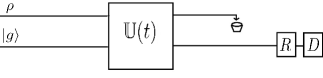
Figure 1: Schematic drawing of the stroboscopic tomographic method discussed in the text. After the field-qubit interaction up to time $t$, a rotation of the qubit state (represented by a box with a R inside) allows to detect the qubit polarization along a selected direction (measurement represented by a box with a D inside).

Our paper is organized as follows. In Sec. II we describe our tomographic method, which is illustrated in Sec. III by several examples: Fock states, superposition of Fock states, coherent states and states generated by the dynamical Casimir effect. Statistical errors due to finite number of measurements are discussed in Sec. IV. Our conclusions are drawn in Sec. V.

II Method

Our state reconstruction method is based on the interaction of a single-mode of the quantized electromagnetic field with a probe qubit. The overall field-qubit system is described by the Jaynes-Cummings hamiltonian micromaser

$$\begin{array}[]{c}{\displaystyle H=H_{0}+H_{I},}\\ \\ {\displaystyle H_{0}=\omega\left(a^{\dagger}a+\frac{1}{2}\right)-\frac{1}{2}\,\omega_{a}\sigma_{z},}\\ \\ {\displaystyle H_{I}=g\,\sigma_{+}a+g^{\star}\sigma_{-}a^{\dagger},}\end{array}$$ (1)

where we set the reduced Planck’s constant $\hbar=1$, $\sigma_{i}$ ($i=x,y,z$) are the Pauli matrices, $\sigma_{\pm}=\frac{1}{2}\,(\sigma_{x}\mp i\sigma_{y})$ are the rising and lowering operators for the qubit: $\sigma_{+}|g\rangle=|e\rangle$, $\sigma_{+}|e\rangle=0$, $\sigma_{-}|g\rangle=0$, $\sigma_{-}|e\rangle=|g\rangle$; the operators $a^{\dagger}$ and $a$ for the field create and annihilate a photon: $a^{\dagger}|n\rangle=\sqrt{n+1}|n+1\rangle$, $a|n\rangle=\sqrt{n}|n-1\rangle$, $|n\rangle$ being the Fock state with $n$ photons. For the sake of simplicity, we consider a real coupling strength, $g\in\mathbb{R}$, and the resonant case, $\omega=\omega_{a}$.

The Jaynes-Cummings model is exactly solvable: in the $\{|g,0\rangle,|e,0\rangle,|g,1\rangle,|e,1\rangle,|g,2\rangle,|e,2\rangle,...\}$ basis we can write the time evolution operator $\mathbb{U}(t)$ up to time $t$ in a block diagonal form:

$$\mathbb{U}(t)=\begin{pmatrix}1&0&0&0&\dots\\ 0&U^{(1)}(t)&0&0&\dots\\ 0&0&U^{(2)}(t)&0&\dots\\ 0&0&0&U^{(3)}(t)&\dots\\ \vdots&\vdots&\vdots&\vdots&\vdots\end{pmatrix}.$$ (2)

Here the interaction picture has been used, the top left matrix element equal to one indicates that the $|g,0\rangle$ state evolves trivially, while the $2\times 2$ matrices

$$U^{(n)}(t)=\begin{pmatrix}U_{11}^{(n)}(t)&U_{12}^{(n)}(t)\\ U_{21}^{(n)}(t)&U_{22}^{(n)}(t)\end{pmatrix}$$

$$=\begin{pmatrix}\cos(\Omega_{n}t)&-i\sin(\Omega_{n}t)\\ -i\sin(\Omega_{n}t)&\cos(\Omega_{n}t)\end{pmatrix}$$ (3)

describe coherent Rabi oscillations between the atom-field states $|g,n\rangle$ and $|e,n-1\rangle$, with the Rabi frequencies $\Omega_{n}=g\sqrt{n}$ ($n=1,2,3,...$).

Our purpose is to obtain information on a generic target state of the field $\rho=\sum_{i,j=0}^{\infty}\rho_{ij}|i\rangle\langle j|$. We assume that the qubit is prepared in its ground state: $\rho^{(q)}=|g\rangle\langle g|$, so that the overall field-qubit state reads $\rho_{\rm tot}=\rho^{(q)}\otimes\rho=|g\rangle\langle g|\otimes\rho$. By evolving such state up to time $t$ under the Jaynes-Cummings Hamiltonian, we have $\rho_{\rm tot}(t)=\mathbb{U}(t)\rho_{\rm tot}\mathbb{U}^{\dagger}$. Tracing over the field we obtain $\rho^{(q)}(t)={\rm Tr}_{f}[\rho_{\rm tot}(t)]$. By means of Eq. (2) we can easily write the matrix elements of $\rho^{(q)}(t)$ as follows:

$$\rho^{(q)}_{gg}(t)=\rho_{00}+\sum_{n=1}^{\infty}U_{22}^{(n)}(t)\rho_{nn}[U_{22}^{(n)}(t)]^{\star}$$

$$=\rho_{00}+\sum_{n=1}^{\infty}\rho_{nn}\cos^{2}(\Omega_{n}t),$$ (4)

$$\rho^{(q)}_{ge}(t)=\rho_{01}[U^{(1)}_{12}(t)]^{\star}+\sum_{n=1}^{\infty}U_{22}^{(n)}(t)\rho_{n,n+1}[U_{12}^{(n+1)}(t)]^{\star}$$

$$=i[\rho_{01}\sin(\Omega_{1}t)+\sum_{n=1}^{\infty}\rho_{n,n+1}\cos(\Omega_{n}t)\sin(\Omega_{n+1}t)].$$ (5)

From the polarization measurements of the probe qubit along the coordinate axes at time $t$ we obtain the Bloch sphere coordinates $x(t),y(t),z(t)$, simply related to the matrix elements of $\rho^{(q)}(t)$ qcbook :

$$\rho^{(q)}_{gg}(t)=\frac{1+z(t)}{2},\quad\rho^{(q)}_{ge}(t)=\frac{x(t)-iy(t)}{2}.$$ (6)

From Eqs. (4), (5), and (6) we obtain

$$z(t)=\rho_{00}+\sum_{n=1}^{\infty}\rho_{nn}\cos(2\Omega_{n}t),$$ (7)

$$x(t)=-\{2\,{\rm Im}(\rho_{01})\sin(\Omega_{1}t)+\sum_{n=1}^{\infty}{\rm Im}(\rho_{n,n+1})[\sin((\Omega_{n+1}+\Omega_{n})t)+\sin((\Omega_{n+1}-\Omega_{n})t)]\},$$ (8)

$$y(t)=-\{2\,{\rm Re}(\rho_{01})\sin(\Omega_{1}t)+\sum_{n=1}^{\infty}{\rm Re}(\rho_{n,n+1})[\sin((\Omega_{n+1}+\Omega_{n})t)+\sin((\Omega_{n+1}-\Omega_{n})t)i]\}.$$ (9)

Finally, the Fourier transforms noteFourier of $x(t)$, $y(t)$, and $z(t)$ are given by

$$\tilde{z}(\omega)=\rho_{00}\delta(\omega)+\frac{1}{2}\,\sum_{n=1}^{\infty}\rho_{nn}[\delta(\omega-2\Omega_{n})+\delta(\omega+2\Omega_{n})],$$ (10)

$$\tilde{x}(\omega)=i\{{\rm Im}(\rho_{01})[\delta(\omega+\Omega_{1})-\delta(\omega-\Omega_{1})]$$

$$+\frac{1}{2}\sum_{n=1}^{\infty}{\rm Im}(\rho_{n,n+1})[\delta(\omega+(\Omega_{n+1}+\Omega_{n}))-\delta(\omega-(\Omega_{n+1}+\Omega_{n}))+\delta(\omega+(\Omega_{n+1}-\Omega_{n}))-\delta(\omega-(\Omega_{n+1}-\Omega_{n}))]\},$$ (11)

$$\tilde{y}(\omega)=i\{{\rm Re}(\rho_{01})[\delta(\omega-\Omega_{1})+\delta(\omega+\Omega_{1})]$$

$$+\frac{1}{2}\sum_{n=1}^{\infty}{\rm Re}(\rho_{n,n+1})[\delta(\omega+(\Omega_{n+1}+\Omega_{n}))-\delta(\omega-(\Omega_{n+1}+\Omega_{n}))+\delta(\omega+(\Omega_{n+1}-\Omega_{n}))-\delta(\omega-(\Omega_{n+1}-\Omega_{n}))]\}.$$ (12)

Hence from the Fourier transform of $z(t)$ we can obtain the populations $\rho_{nn}$ of the target (initial) state of the field, while from the Fourier transform of $x(t)$ and $y(t)$ we can reconstruct the coherences $\rho_{n,n+1}$ ($n=0,1,...$). This information is in general sufficient to fully reconstruct a pure state

$$|\psi\rangle=\sum_{n=0}^{\infty}c_{n}|n\rangle=\sum_{n=0}^{\infty}|c_{n}|e^{i\phi_{n}}|n\rangle.$$ (13)

Indeed in this case $|c_{n}|=\sqrt{\rho_{nn}}$, while

$$\rho_{n,n+1}=c_{n}c_{n+1}^{\star}=|c_{n}||c_{n+1}|e^{i(\phi_{n}-\phi_{n+1})}.$$ (14)

Knowing $|c_{n}|$ and $|c_{n+1}|$ from the populations $\rho_{nn}$ and $\rho_{n+1,n+1}$ (i.e., from the measurements of the qubit polarization along $z$), we can derive the relative phase $\phi_{n,n+1}\equiv\phi_{n}-\phi_{n+1}$, and therefore fully reconstruct the state $|\psi\rangle$. This method for pure states only fails in the particular cases where there exist two coefficients $c_{j},c_{l}\neq 0$ and in between a vanishing coefficient $c_{k}=0$ ($j<k<l$), as, for instance, in a state like $|c_{0}||0\rangle+|c_{2}|e^{i\phi_{02}}|2\rangle$. In this case, our method only allows us to determine the populations $|c_{0}|,|c_{2}|$ but not the relative phase $\phi_{02}$.

III Examples

We illustrate the general method of Sec. II in a few examples ordered by growing complexity. Note that the equations reported below are instances of the general expressions (10)-(12).

III.1 Fock states

In this case $\rho=|n\rangle\langle n|$ and $\tilde{z}(\omega)=\frac{1}{2}\,[\delta(\omega-2\Omega_{n})+\delta(\omega+2\Omega_{n})]$ for $n\neq 0$, while $\tilde{z}(\omega)=\delta(\omega)$ for $n=0$. On the other hand, $\tilde{x}(\omega)=\tilde{y}(\omega)\equiv 0$ as coherences are zero for this state.

III.2 Superposition of Fock states

Let us consider two particular cases, showing that the method is useful to reproduce not only the populations but also the coherences of a state. We consider $\frac{1}{\sqrt{2}}\,(|1\rangle+|2\rangle)$ (state $1$) and $\frac{1}{\sqrt{2}}\,(|1\rangle+e^{i\pi/4}|2\rangle)$ (state $2$). Let $(x_{i},y_{i},z_{i})$ denote the Bloch vector for state $i$ ($i=1,2$). The two states have the same populations and

$$\tilde{z}_{1}(\omega)=\tilde{z}_{2}(\omega)=\frac{1}{4}\,[\delta(\omega-2\Omega_{1})+\delta(\omega+2\Omega_{1})$$

$$+\delta(\omega-2\Omega_{2})+\delta(\omega+2\Omega_{2})].$$ (15)

The first state is real and therefore $\tilde{x}_{1}(\omega)=0$, while

$$\tilde{y}_{1}(\omega)=\frac{i}{4}\,[\delta(\omega+(\Omega_{1}+\Omega_{2}))-\delta(\omega-(\Omega_{1}+\Omega_{2}))$$

$$+\delta(\omega+(\Omega_{2}-\Omega_{1}))-\delta(\omega-(\Omega_{2}-\Omega_{1}))].$$ (16)

On the other hand, for the second state ${\rm Re}(\rho_{12})={\rm Im}(\rho_{12})$ and we have $\tilde{x}_{2}(\omega)=\tilde{y}_{2}(\omega)=\frac{\sqrt{2}}{2}\,\tilde{y}_{1}(\omega)$.

These results are illustrated in Fig. 2, where we simulate an experiment repeated for $N_{t}=4096$ interaction times $t_{k}$, separated by a time step $\Delta t=0.075/\Omega_{1}$, assuming that for each time $t_{k}$ an ideally unlimited number of experimental runs is performed (the impact of statistical errors due to finite number of measurements will be discussed in Sec. IV). Due to the finite maximum interaction time $T=N_{t}(\Delta t)$, the delta functions of the above expressions are broadened. Nevertheless, by measuring the overall area below the peaks we can reconstruct with very good accuracy (three significant digits) the non-zero matrix elements of the density operator $\rho$ for the two states, see the table below. For instance, by adding the areas below the peaks at $\omega=2\Omega_{1}$ and $\omega=-2\Omega_{1}$ in $\tilde{z}_{1}=\tilde{z}_{2}$ we obtain $\rho_{11}=0.5004$, to be compared with the exact value $\rho_{11}=\frac{1}{2}$. For the state $\rho_{2}$, we obtain from $\tilde{x}_{2}$ and $\tilde{y}_{2}$ that ${\rm Re}[\rho_{12}]={\rm Im}[\rho_{12}]=0.3532$, to be compared with the exact value ${\rm Re}[\rho_{12}]={\rm Im}[\rho_{12}]=1/2\sqrt{2}\approx 0.3536$.

	state $1$	state $2$
$\rho_{11}$	0.5004	0.5004
$\rho_{22}$	0.4997	0.4997
Re$[\rho_{12}]$	0.4998	0.3532
Im$[\rho_{12}]$	0	0.3532

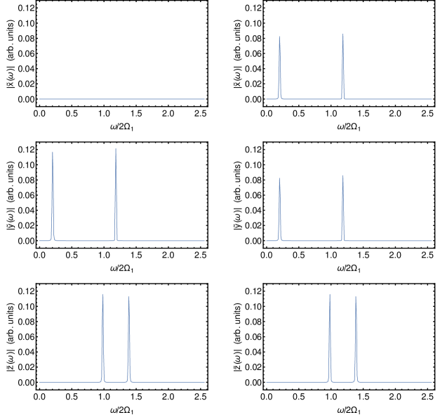
Figure 2: Fourier transforms $\tilde{x}(\omega)$, $\tilde{y}(\omega)$, and $\tilde{z}(\omega)$ of the Bloch sphere coordinates of the probe qubit, for the field input states $\frac{1}{\sqrt{2}}\,(|1\rangle+|2\rangle)$ (left) and $\frac{1}{\sqrt{2}}\,(|1\rangle+e^{i\pi/4}|2\rangle)$ (right). Note that we only show the Fourier transforms for $\omega>0$, since they are symmetric for $\omega\to-\omega$.

III.3 Coherent states

We now consider a coherent state, whose representation in the basis of Fock states reads $|\alpha\rangle=\sum_{n=0}^{\infty}c_{n}|n\rangle$, where $c_{n}=\exp\left(-\frac{|\alpha|^{2}}{2}\right)\frac{\alpha^{n}}{\sqrt{n!}}$, with $\alpha\in\mathbb{C}$. In the simulations reported below we use a complex value $\alpha=0.7e^{i\pi/3}$ to demonstrate that not only populations but also coherences of the field can be measured. In the bottom panel of Fig. 3 we can clearly see the peaks at $\omega=2\Omega_{n}$ for $n=0,1,2,3$, corresponding to $\omega/2\Omega_{1}=0,1,\sqrt{2},\sqrt{3}$, respectively. By integrating the areas below these peaks (and the symmetric peaks at $\omega=-2\Omega_{n}$ not shown here) we reconstruct the populations $\rho_{nn}$. The coherences $\rho_{n,n+1}$ are then obtained from the areas below the peaks in $\tilde{x}(\omega)$ and $\tilde{y}(\omega)$ in Fig. 3. The relative phases $\phi_{n}-\phi_{n+1}$ are then derived via Eq. (14). Finally, all the phases $\phi_{n}$ are obtained once the overall arbitrary phase is set, for instance we can choose $\phi_{0}=0$. Knowing $|c_{n}|=\sqrt{\rho_{nn}}$ and $\phi_{n}$, we have fully reconstructed the field state. The good agreement between the results obtained by means of our tomographic method and the exact field state is shown in Fig. 4.

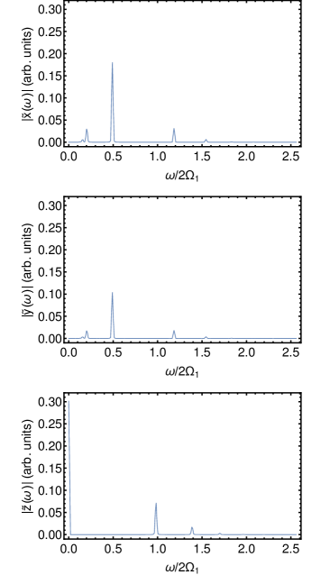
Figure 3: As in 2 but for a coherent state with $\alpha=0.7e^{i\pi/3}$.

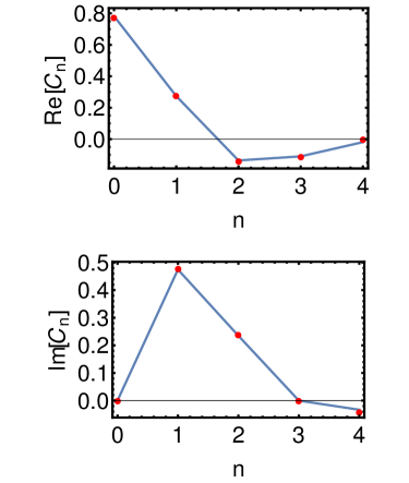
Figure 4: Real and imaginary part of a coherent state with $\alpha=0.7e^{i\pi/3}$ (line) and state reconstruction by means of the Fourier transforms $\tilde{x}(\omega)$, $\tilde{y}(\omega)$, and $\tilde{z}(\omega)$ of Fig. 3 (circles).

III.4 Exotic states from the dynamical Casimir effect

The Dynamical Casimir Effect (DCE) moore ; dodonov ; noriRMP is the generation of photons from the vacuum due to time-dependent boundary conditions for the electromagnetic field. Such quantum vacuum amplification effect has been observed in experiments with superconducting circuits norinature ; lahteenmaki , and also investigated in the context of Bose-Einstein condensates jaskula , in exciton-polariton condensates koghee , for multipartite entanglement generation in cavity networks solano2014 ; savasta , for quantum communication protocols casimirqip , for quantum technologies adesso and also in the context of finite-time quantum thermodynamics frigo .

The field state we want to reconstruct by means of our tomographic protocol is obtained from the interaction between a two-level system and a single mode of the quantized electromagnetic field, described by the time-dependent Rabi Hamiltonian micromaser

$$\begin{array}[]{c}{\displaystyle H(t)=H_{0}+H_{I}(t),}\\ \\ {\displaystyle H_{0}=\omega\left(a^{\dagger}a+\frac{1}{2}\right)-\frac{1}{2}\,\omega_{a}\sigma_{z},}\\ \\ {\displaystyle H_{I}(t)=f(t)\,[\,g\,\sigma_{+}\,(a^{\dagger}+a)+g^{\star}\sigma_{-}\,(a^{\dagger}+a)\,],}\end{array}$$ (17)

where we assume sudden switch on/off of the coupling: $f(t)=1$ for $0\leq t\leq\tau$, $f(t)=0$ otherwise footparametric . It is the non-adiabatic switching of the interaction that leads to the DCE, namely to the generation of photons even though initially both the field and the qubit are in their ground state. Hamiltonian (17) leads to the generation of exotic states of the field with negative components in their Wigner function exotic . Such states are very different from the squeezed states obtained in approximate descriptions of the DCE via quadratic Hamiltonians bastard ; noriRMP .

We consider as initial condition the state $|\Psi_{0}\rangle=|g,0\rangle$ and compute numerically the qubit-field state after the interaction time: $|\Psi(\tau)\rangle=c_{g}(\tau)|g\rangle|\phi_{g}(\tau)\rangle+c_{e}(\tau)|e\rangle|\phi_{e}(\tau)\rangle$, where $|\phi_{g}\rangle$ and $|\phi_{e}\rangle$ are normalized states of the field. Note that we define the initial state $|g,0\rangle$ before switching on the interaction and consider the final state $|\Psi(\tau)\rangle$ after the interaction has been switched off. By changing the interaction strength $g$ and the interaction time $\tau$ we can generate a great variety of states of the field exotic , both in the unconditional case and in the conditional case in which the final qubit state is measured, for instance in the $\{|g\rangle,|e\rangle\}$ basis. In the first case, the field state reads $\rho={\rm Tr}_{q}|\Psi\rangle\langle\Psi|=|c_{g}|^{2}|\phi_{g}\rangle\langle\phi_{g}|+|c_{e}|^{2}|\phi_{e}\rangle\langle\phi_{e}|$, where ${\rm Tr}_{q}$ denotes the trace over the qubit subsystem; in the latter case, we obtain the (pure) states $\rho_{g}=|\phi_{g}\rangle\langle\phi_{g}|$ or $\rho_{e}=|\phi_{e}\rangle\langle\phi_{e}|$.

As illustrated in Fig. 5, the states $\rho_{g}$ and $\rho_{e}$ can be reconstructed via the tomographic method introduced in this paper. There is, however, a catch: since the parity $\Pi=\sigma_{z}(-1)^{a^{\dagger}a}$ of the excitations is conserved by the Rabi Hamiltonian, for the conditional states $\rho_{g}$ and $\rho_{e}$ only the Fock states with respectively an even and an odd number of photons are populated. We are therefore in the situation in which in the expansions of $|\phi_{g}\rangle$ and $|\phi_{e}\rangle$ on the Fock basis there exist vanishing coefficients between non-zero coefficients and therefore our tomographic method would fail. However, this problem can be overcome if the conditional states are obtained after measuring in the $\{|+\rangle,|-\rangle\}$ basis, with $|\pm\rangle=\frac{1}{\sqrt{2}}\,(|g\rangle\pm|e\rangle)$, rather than in the $\{|g\rangle,|e\rangle\}$ basis. We first of all rewrite $|\Psi(\tau)\rangle$ as follows:

$$|\Psi(\tau)\rangle=\frac{1}{\sqrt{2}}\,(|\phi_{+}(\tau)\rangle|+\rangle+|\phi_{-}(\tau)\rangle|-\rangle),$$ (18)

where we have defined

$$|\phi_{\pm}(\tau)\rangle=c_{g}(\tau)|\phi_{g}(\tau)\rangle\pm c_{e}(\tau)|\phi_{e}(\tau)\rangle.$$ (19)

After the measurement of the qubit in the $\{|+\rangle,|-\rangle\}$ basis, we obtain with equal probability $p_{+}=p_{-}=\frac{1}{2}$ either the field state $\rho_{+}=|\phi_{+}\rangle\langle\phi_{+}|$ or $\rho_{-}=|\phi_{-}\rangle\langle\phi_{-}|$. These conditional pure states have non-zero components in the Fock basis both for even and odd number of photons and can therefore be reconstructed by our tomographic method. We finally obtain $|\phi_{g}\rangle=\frac{1}{2c_{g}}\,(|\phi_{+}\rangle+|\phi_{-}\rangle)$ and $|\phi_{e}\rangle=\frac{1}{2c_{e}}\,(|\phi_{+}\rangle-|\phi_{-}\rangle)$. An example of the reconstruction of the states $|\phi_{g}\rangle$ and $|\phi_{e}\rangle$ is shown in Fig. 6. We finally note that also the unconditional state $\rho=|c_{g}|^{2}|\phi_{g}\rangle\langle\phi_{g}|+|c_{e}|^{2}|\phi_{e}\rangle\langle\phi_{e}|$ can be reconstructed, with $p_{g}=|c_{g}|^{2}$ and $p_{e}=|c_{e}|^{2}$ probabilities of the outcomes $g$ and $e$ when the qubit is measured in the $\{|g\rangle,|e\rangle\}$ basis.

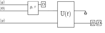
Figure 5: State reconstruction of field states generated by the dynamical Casimir effect, with field-qubit interaction strength $g$ and interaction time $\tau$. Pure states of the field are then obtained after measurement of the qubit polarization and analyzed via the state reconstruction method described in this paper, with $\mathbb{U}(t)$ time evolution operator corresponding to the Jaynes-Cummings interaction of the field with a probe qubit up to time $t$.

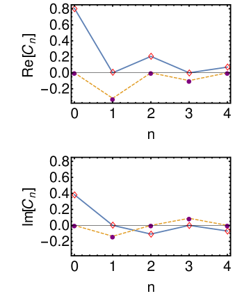
Figure 6: Real and imaginary part of the states $|\phi_{g}(\tau)\rangle$ (full line and diamonds) and $|\phi_{e}(\tau)\rangle$ (dashed line and circles) in the dynamical Casimir effect with $\omega=\omega_{a}$, $g/\omega=0.5$ and interaction time $\tau=\pi/2g$. Lines stand for the exact results, symbols for the data obtained by state reconstruction.

IV Statistical errors

We now consider the realistic situation where at each discrete time $t_{k}=k(\Delta t)$ ($k=1,2,...,N_{t}$) a finite number $N_{m}$ of measurements is performed and the average of the measurement outcomes is computed. For each measurement, the system is initially prepared in the same unknown targed state $\rho$ and evolves (interacting with the qubit) till time $t_{k}$, where the polarization of the qubit, say along the $z$-axis, is measured. As a result, for each experimental run we obtain either $+1$ or $-1$ from the polarization measurement, with the a priori probabilities set by the postulates of quantum mechanics. The actually measured polarization $z_{M}(t_{k})$ is then the sum of two parts, the polarization expectation value $z(t_{k})$ (recovered in the limit $N_{m}\to\infty$) and the “noise” $z_{N}(t_{k})$ (due to finite $N_{m}$), which can be modeled as a white noise of root mean square (RMS) amplitude $1/\sqrt{N_{m}}$. The Fourier transform of the white noise is flat and its RMS amplitude is given by $\xi\propto 1/\sqrt{N_{m}}$, independently of $N_{t}$. On the other hand, if we keep $\Delta t$ constant and increase both $N_{t}$ and $T=N_{t}(\Delta t)$, we expect that the signal (peak area in the Fourier transform) increases proportionally to the number of time intervals, while the noise, being random, increases as $\sqrt{N_{t}}$. Therefore the signal to noise ration $S/\xi$ increases as $\sqrt{N_{t}}$.

The above expectations are confirmed by the numerical simulation of the simplest instance of state reconstruction, namely a Fock state, here $\rho=|1\rangle\langle 1|$. The Fourier transform of $z_{M}(t)$ shows a peak corresponding to $\omega=\Omega_{1}$ and a flat noise, see Fig. 7 top panel (the symmetric peak at $\omega=-\Omega_{1}$ is not shown in the figure). Finally, in the bottom plots of Fig. 7 we show that the RMS noise amplitude $\xi\propto 1/\sqrt{N_{m}}$, while the signal over noise ratio $S/\xi\propto\sqrt{N_{t}}$. Note that in the above estimates we have assumed for the sake of simplicity the maximum statistical error. Such error can be smaller depending on the signal amplitude. For instance, for a signal such that $z=+1$ (or $z=-1$) the measurement has a constant value and statistical fluctuations vanish.

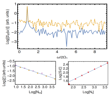
Figure 7: Top: Fourier transform of $z_{M}(t)$ for $T=20\pi/\Omega_{1}$, $N_{t}=512$, and $N_{m}=10$ (dashed curve) and $1000$ (solid curve). Bottom left: root mean square noise amplitude as a function of the number of measurements $N_{m}$, for $T=20\pi/\Omega_{1}$, $N_{t}=128$ (squares) and $N_{t}=1024$ (triangles). The straight line corresponds to $\xi\propto 1/\sqrt{N_{m}}$ Bottom right: signal over noise ratio $S/\xi$ as function of $N_{t}$, for $\Delta t=0.075/\Omega_{1}$, $N_{m}=1000$. The straight line gives the theoretical dependence $S/\xi\propto\sqrt{N_{t}}$. In all panels the logarithms are base 10.

In a real experiment, decoherence effects would damp the oscillations in the Bloch sphere coordinates. Assuming a simple exponential decay, $z(t)\propto e^{-\Gamma t}$, the peaks in the Fourier transform $\tilde{z}(\omega)$ broaden but can still be resolved, provided the decay rate $\Gamma$ is sufficiently smaller than the separation $\Delta\omega$ between nearby peaks footnote2 .

V Conclusions

In this paper, we have introduced a new tomographic method for state reconstruction of a single mode of the electromagnetic field by means of its interaction with a probe qubit. The qubit polarizations $x(t)$, $y(t)$, and $z(t)$ along three coordinate axes are then measured at different times $t$ and from their Fourier transforms $\tilde{x}(\omega)$, $\tilde{y}(\omega)$, and $\tilde{z}(\omega)$ one can in general fully reconstruct pure states of the field and obtain partial information in the case of mixed states. That is, one can reconstruct the diagonal and the superdiagonal of the density matrix $\rho$. The method could in principle be generalized, at the expense of a higher complexity but with a richer information of the state $\rho$, by using probe qudits rather than qubits coherently interacting with the field. Our method could also implement a simple instance of process state tomography. That is, assuming a field-qubit Jaynes-Cummings interaction with unknown interaction strength $g$, one could use the position of the peaks in the Fourier transforms $\tilde{x}(\omega)$, $\tilde{y}(\omega)$, and $\tilde{z}(\omega)$ to determine $g$. On a more general perspective, the method described in this paper has some similarities with the quantum algorithm proposed by Abrams and Lloyd Lloyd for finding eigenvalues and eigenvectors of an Hamiltonian operator. Both in the quantum algorithm of Ref. Lloyd and in the state reconstruction procedure described in this paper, the quantities of interest (the eigenvalues and the eigenvectors or the density matrix elements, respectively) are hidden in the time evolution of a suitable system and then extracted by means of the Fourier transform.

- (1) U. Fano, Rev. Mod. Phys. 29, 74 (1957).
- (2) An Hermitian matrix has independent elements, but the unit trace condition removes one of them.
- (3) G. M. D’Ariano, M. G. A. Paris, and M. F. Sacchi, in Advances in Imaging and Electron Physics, Vol. 128, p. 205-308 (2003).
- (4) M. G. A. Paris and J. Řeháček (Eds.), Quantum State Estimation, Lecture Notes in Physics, Vol. 649 (Springer, Berlin Heidelberg, 2004)
- (5) G. M. D’Ariano, L. Maccone, and M. F. Sacchi, in Quantum information with continuous variables of atoms and light, N. J. Cerf, G. Leuchs, and E. S. Polzik (Eds.) (World Scientific, Singapore, 2007)
- (6) A. I. Lvovsky and M. G. Raymer, Rev. Mod. Phys. 81, 299 (2009).
- (7) S. N. Filippov, V. I. Man’ko, Phys. Scr. 3, 058101 (2011).
- (8) P. Meystre and M. Sargent III, Elements of quantum optics (4th Ed.) (Springer–Verlag, Berlin, 2007).
- (9) G. Benenti, G. Casati, and G. Strini, Principles of Quantum Computation and Information, Vol. I: Basic concepts (World Scientific, Singapore, 2004); Vol. II: Basic tools and special topics (World Scientific, Singapore, 2007).
- (10) While for the sake of simplicity in what follows we shall write formulas for the Fourier transform of a continuous signal, one should more precisely consider the discrete Fourier transform, the measurements being performed only at discrete times up to a finite interaction time (see the examples of Secs. III and IV).
- (11) G. T. Moore, J. Math. Phys. (N.Y.) 11, 2679 (1970).
- (12) V. V. Dodonov, Phys. Scripta 82, 038105 (2010).
- (13) P. D. Nation, J. R. Johansson, M. P. Blencowe, and F. Nori, Rev. Mod. Phys. 84, 1 (2012).
- (14) C. M. Wilson, G. Johansson, A. Pourkabirian, M. Simoen, J. R. Johansson, T. Duty, F. Nori, and P. Delsing, Nature (London) 479, 376 (2011).
- (15) P. Lähteenmäki, G. S. Paraoanu, J. Hassel, and P. J. Hakonen, PNAS 110, 4234 (2013).
- (16) J.-C. Jaskula, G. B. Partridge, M. Bonneau, R. Lopes, J. Ruaudel, D. Boiron, and C. I. Westbrook, Phys. Rev. Lett. 109, 220401 (2012).
- (17) S. Koghee and M. Wouters, Phys. Rev. Lett. 112, 036406 (2014).
- (18) S. Felicetti, M. Sanz, L. Lamata, G. Romero, G. Johansson, P. Delsing, and E. Solano, Phys. Rev. Lett. 113, 093602 (2014).
- (19) R. Stassi, S. De Liberato, L. Garziano, B. Spagnolo, and S. Savasta, Phys. Rev. A 92, 013830 (2015).
- (20) G. Benenti, A. D’Arrigo, S. Siccardi, and G. Strini, Phys. Rev. A 90, 052313 (2014).
- (21) C. Sabín and G. Adesso, Phys. Rev. A 92, 042107 (2016).
- (22) G. Benenti and G. Strini, Phys. Rev. A 91, 020502(R) (2015).
- (23) Alternatively and with results analogous to those discussed in this paper, the time dependence can be considered in the detuning rather than in the coupling constant.
- (24) G. Benenti, S. Siccardi, and G. Strini, Eur. Phys. J. D 68, 139 (2014).
- (25) C. Ciuti, G. Bastard, and I. Carusotto, Phys. Rev. B 72, 115303 (2005).
- (26) A more detailed analysis is required when low-frequency non-Markovian noise is relevant, see for instance nmarkov1 ; nmarkov2 ; nmarkov3 .
- (27) G. Falci, A. D’Arrigo, A. Mastellone, and E. Paladino Phys. Rev. Lett. 94, 167002 (2005).
- (28) A. D’Arrigo, R. Lo Franco, G. Benenti, E. Paladino, and G. Falci, Ann. Phys. 350, 211 (2014).
- (29) A. Orieux, A. D’Arrigo, G. Ferranti, R. Lo Franco, G. Benenti, E. Paladino, G. Falci, F. Sciarrino, and P. Mataloni, Sci. Rep. 5, 8575 (2015).
- (30) D. S. Abrams and S. Lloyd, Phys. Rev. Lett. 83, 5162 (1999).