Grain size correlated rotatable magnetic anisotropy in polycrystalline exchange bias systems

Abstract

Angular resolved measurements of the exchange bias field and the coercive field are a powerful tool to distinguish between different competing magnetic anisotropies in polycrystalline exchange bias layer systems. No simple analytical model is as yet available, which considers time dependent effects like enhanced coercivity arising from the grain size distribution of the antiferromagnet.
In this work we expand an existing model class describing polycrystalline exchange bias systems by a rotatable magnetic anisotropy term to describe grain size correlated effects. Additionally, we performed angular resolved magnetization curve measurements using vectorial magnetooptic Kerr magnetometry. Comparison of the experimental data with the proposed model shows excellent agreement and reveals the ferromagnetic anisotropy and properties connected to the grain size distribution of the antiferromagnet. Therefore, a distinction between the different influences on coercivity and anisotropy becomes available.

I Introduction

Exchange bias (EB), firstly discovered by Meiklejohn and Bean in 1956Meiklejohn and Bean (1956, 1957), is a magnetic interface effect between a ferromagnetic (F) and an antiferromagnetic (AF) layerMeiklejohn and Bean (1956). The exchange interaction between individual magnetic moments of the F and the AF across the interface leads to unidirectionalMeiklejohn and Bean (1956) and rotatable magnetic anisotropyGeshev et al. (2002); Kim et al. (2003); Radu and Zabel (2008) in the F. EB is nowadays widely used in magnetic sensor heads to pin the magnetization direction of the magnetic reference electrodeNogu s and Schuller (1999). Recently, new interest in an improved description of the EB effect aroseEhresmann et al. (2015) as ion bombardment induced magnetic patterning of EB layer systems allows tailoring artificial magnetic stray field landscapesEhresmann et al. (2006) which are very likely to be a central part of magnetic particle transport in lab-on-chip applications for, e.g., biosensingEhresmann et al. (2011a); Holzinger et al. (2015); Ehresmann et al. (2015).
Although the EB effect was investigated for almost 60 years, a complete theoretical description is still not available. Recently, a promising modelO’Grady et al. (2010) for polycrystalline magnetic thin films was developed, which detailed similar earlier ideasSoeya et al. (1996); Ehresmann et al. (2005). This model takes into account the granular structure of a polycrystalline AFFulcomer and Charap (1972), dividing grains into categoriesSoeya et al. (1996) based on their individual relaxation times

$$\tau_{\mathrm{i}}=\frac{1}{f_{0}}\exp\left[-\frac{\Delta E}{k_{\mathrm{B}}T}\right],\Delta E=K_{\mathrm{AF,i}}V_{\mathrm{AF,i}}.$$ (1)

Here, $f_{0}$ is the characteristic frequency for spin reversalVallejo-Fernandez et al. (2010), $T$ is the temperature and $k_{\mathrm{B}}$ is Boltzmann’s constant. $\Delta E$ is the energy barrier between a local and a global energy minimum in the potential energy landscape as a function of angle between F and pinned AF momentEhresmann et al. (2005). In first order, it can be written as the product of magnetic anisotropy $K_{\mathrm{AF,i}}$ and volume $V_{\mathrm{AF,i}}$ of the respective grains. Polycrystalline layer systems typically show a distribution of grain sizesVallejo-Fernandez et al. (2008), resulting in a distribution of relaxation times over several orders of magnitudeO’Grady et al. (2010).
Thermal stability of grains may be defined by comparing the relaxation time to the measurement conditionsO’Grady et al. (2010), leading to a classification of grains into categoriesSoeya et al. (1996); Ehresmann et al. (2011b) as shown in figure 1.

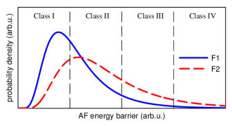
Figure 1: Schematic probability distribution of energy barriers in AF grains. F1 and F2 are lognormal functions related to systems with a different average energy barrier. AF grains may be divided into four categories (see text) depending on their energy barriers.

Grains with small energy barriers reorient during a magnetization curve cycle. They can be divided into superparamagnetic grainsEhresmann et al. (2011b) showing the smallest energy barriers (Class I) and coercivity mediating grainsO’Grady et al. (2010) (Class II). Only grains with higher energy barriers having a relaxation time longer than the measurement time are able to contribute to the EB field $H_{\mathrm{EB}}$O’Grady et al. (2010). The contribution of these thermally stable grains to the direction of $H_{\mathrm{EB}}$ is random, as long as they are not set by a magnetic field cooling processO’Grady et al. (2010) or a similar procedureEngel et al. (2005); Harres and Geshev (2012). They can be divided further into grains, which reorient during the field cooling process yielding a macroscopic contribution to $H_{\mathrm{EB}}$ (Class III) and the grains with the highest energy barrier (Class IV), which are even stable at the field cooling conditions.
In addition to the influence of the AF layer on the EB, the magnetic anisotropy of the F layer itself is another fundamental property defining the behavior of the system. For the characterization of EB samples the influences of the different magnetic anisotropy termsCamarero et al. (2005) have to be distinguished. Angular resolved measurementsAmbrose et al. (1997) of $H_{\mathrm{EB}}$ and the coercive field $H_{\mathrm{C}}$ (see figure 2) may be used to disentangle the influences of the distributions of the different magnetic anisotropiesHoffmann et al. (2003); Camarero et al. (2005), if these measurements are compared to numerical calculations, e.g., based on the model of Stoner and WohlfarthStoner and Wohlfarth (1947, 1948). With this approach material constants and the mutual direction of different magnetic anisotropy contributions are visualizedJiménez et al. (2009).
In none of these numerical models, however, the relaxation time distributionO’Grady et al. (2010) of the AF grains is considered. Although this may not be necessary at low temperature, where some of the fundamental experiments have been carried out, applications of the EB systems usually take place at room temperature (RT). A proper characterization, therefore, needs to be performed at RT, where thermal activation processes can not be neglectedO’Grady et al. (2010). To reveal the impact of Class II grains the typical procedure of measuring magnetic easy axis hysteresis loops is not sufficient for EB systems possessing non negligible magnetic anisotropy of the F layer, since the two sources of coercivity can not be distinguished.

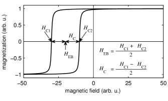
Figure 2: Schematic view of a magnetization curve of an EB layer system. The characteristic quantities exchange bias field $H_{\mathrm{EB}}$ (the curve shift) and coercive field $H_{\mathrm{C}}$ (the broadness of the hysteretic curve) are calculated with the two coercive fields $H_{\text{C1}}$ and $H_{\text{C2}}$, at which the magnetization along the measurement direction equals zero.

Our numerical calculations are based on the model of Stoner and WohlfarthStoner and Wohlfarth (1947, 1948). Thermal effectsFulcomer and Charap (1972); O’Grady et al. (2010) are introduced by taking into account a rotatable magnetic anisotropy term related to the grain size. Further, we apply angle-resolved magnetization curve measurements using the magnetooptic Kerr effect (MOKE) to determine $H_{\mathrm{EB}}$ and $H_{\mathrm{C}}$ as a function of angle for a model system consisting of an Ir₁₇Mn₈₃/Co₇₀Fe₃₀ bilayer. By comparing these results to the numerical model it is possible to reveal the magnetic properties of the system, including the effects arising from thermally unstable parts of the AF, by distinguishing the different sources of coercivity. Further we show the impact of the measurement time on $H_{\mathrm{EB}}$ and $H_{\mathrm{C}}$ as a function of angle to prove the validity of the proposed model.

II Experimental

II.1 Sample preparation

The EB bilayer system of Ir₁₇Mn₈₃${}^{30~{}\mathrm{nm}}$/Co₇₀Fe₃₀${}^{15~{}\mathrm{nm}}$ was deposited on a naturally oxidized Si(100) substrate using rf-sputter deposition at room temperature with an applied in-plane magnetic field of 60 kA/m, where the base pressure was $10^{-6}$ mbar and the working pressure $2\cdot 10^{-2}$ mbar. A 50 nm Cu buffer layer was used to induce the (111) texture in the Ir₁₇Mn₈₃Aley et al. (2008). For the AF a layer thickness of 30 nm was chosen to enhance the AF grain volume delivering high thermal stability O’Grady et al. (2010) with reduced thermal activation. A Si capping layer with a thickness of 20 nm was used to protect the EB bilayer from oxidation and for enhanced contrast in magnetooptic measurements Nakamura et al. (1985).
The EB system subsequently was annealed at 573.15 K for 60 min in an external in-plane magnetic field of 80 kA/m to maximize the macroscopic $H_{\mathrm{EB}}$. Afterwards the samples were cooled down in this field to room temperature at a rate of 5 K/min.

II.2 Magnetooptic Kerr effect measurements

Samples were investigated by vectorial magnetooptic Kerr magnetometry in an extended MOKE setup similar to the one described in Ref.Kuschel et al. (2011). $p$-polarized light from a laser operating at a central wavelength of 632 nm was used to illuminate the sample. The reflected light was analyzed by a detector system yielding the reflectivity and the Kerr angle of the sample. The Kerr angle, in case of an in-plane magnetized sample, refers to the longitudinal Kerr effect and, therefore, is directly proportional to the magnetization component parallel to the applied magnetic fieldHubert and Schäfer (1998). The reflectivity of the sample yields direct proportionality to the transverse magnetization component. Normalizing both components with respect to the saturation magnetization allows reconstruction of the magnetization vector Vavassori (2000).
The sample is mounted on a rotatable sample stage in order to perform angular resolved measurements within the sample plane. Magnetization curves were obtained over an external magnetic field angle range of 360^∘  with a resolution of 2^∘ applying an external magnetic field divided into 300 steps per branch with a maximum magnetic field of 80 kA/m. Due to enhanced magnetooptic effects arising from the silicon capping layer, no averaging of magnetization curves was necessary.
For the time dependent measurements one set of magnetization curve measurements was recorded for different measurement times $T_{\mathrm{H}}$ for one magnetization curve. In each set of measurements $T_{\mathrm{H}}$ was kept constant and the external magnetic field angle was varied in a range of 180^∘ with a resolution of 2^∘. $T_{\mathrm{H}}$ was selected between 17 seconds and 5 minutes. The sets were measured in a random order to make sure that the training effect is not the main reason for the observed changes in the magnetization curves.

III Model

For the numerical calculations of the magnetization curves a Stoner-Wohlfarth-like model was used, where the magnetization of the F $\vec{M}$ was assumed to be uniform Stoner and Wohlfarth (1947). This holds as long as the magnetization reversal of the systems occurs via coherent rotation. However, for magnetization curve measurements along the magnetic easy axis of the system the magnetization reversal takes place via nucleation and/or domain wall motion McCord et al. (2003), so deviations in this regime are expected. Due to strong shape anisotropy of thin film EB systems the magnetization was assumed to be parallel to the surface.
To determine the magnetization direction of the F layer a potential energy landscape is calculated as a function of $\beta_{\mathrm{F}}$, which is the angle between $\vec{M}$ and the x-axis of the coordinate system (see figure 3). The potential energy landscape per area $A$ is minimized with respect to $\beta_{\mathrm{F}}$. For the case of more than one minimum the magnetization direction is derived with the perfect delay convention Nieber and Kronmüller (1991). Therefore, only that energetic states are taken into consideration, which are reachable via rotation from the starting point of the $\beta_{\mathrm{F}}$  variation without overcoming an energy barrier.
The potential energy landscape consists of several magnetic anisotropy terms which define the behavior of the system (see figure 3 for a graphical illustration) and the Zeeman term $E_{\mathrm{Z}}$, describing the interaction of the magnetic layer with the external magnetic field with

$$E_{\mathrm{Z}}/A=\mu_{0}H_{\mathrm{ext}}M_{\mathrm{sat}}t_{\mathrm{F}}\cos{\left(\beta_{\mathrm{F}}-\varphi_{\mathrm{ext}}\right)}.$$ (2)

Here, $\mu_{0}$ is the magnetic permeability in vacuum, $M_{\mathrm{sat}}$ the saturation magnetization of the F and $t_{\mathrm{F}}$ its thickness, $H_{\mathrm{ext}}$ the strength of the external magnetic field and $\varphi_{\mathrm{ext}}$ the angle describing its in-plane direction.

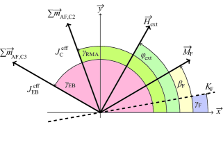
Figure 3: Graphical illustration of the angles and vectors used in the proposed model in a polar coordinate system. $\vec{M}_{\mathrm{F}}$ is the magnetization vector of the F layer and $\beta_{\mathrm{F}}$ its azimuth. $K_{\mathrm{F}}$ is the energy density per unit area of the uniaxial magnetic anisotropy (UMA) of the F and $\gamma_{\mathrm{F}}$ the azimuth of its magnetic easy direction. $\vec{H}_{\mathrm{ext}}$ is the external magnetic field vector with the azimuth $\varphi_{\mathrm{ext}}$. $\vec{m}_{\mathrm{AF,C2}}$ and $\vec{m}_{\mathrm{AF,C3}}$ are the surface magnetization moments associated to AF grains of Class II and III respectively. $\gamma_{\mathrm{RMA}}$ and $\gamma_{\mathrm{EB}}$ are the corresponding azimuths of the vector sums, which are connected to the rotatable and unidirectional magnetic anisotropies with the respective surface energy densities $J_{\mathrm{C}}^{\mathrm{eff}}$ and $J_{\mathrm{EB}}^{\mathrm{eff}}$.

The intrinsic magnetic anisotropy $E_{\mathrm{uni}}$ of the F layer was assumed to be uniaxialKim et al. (2006). This is valid, although the magneto-crystalline anisotropy of CoFe is biaxial Öksüzoğlu et al. (2011); Kuschel et al. (2012), because the uniaxial magnetic anisotropy (UMA) induced by the field cooling process is dominant. This was also confirmed in preparatory investigations (not shown), where angle-resolved vector MOKE measurements with a pure Co₇₀Fe₃₀ layer were performed. The energy area density of the UMA results in

$$E_{\mathrm{uni}}/A=K_{\mathrm{F}}t_{\mathrm{F}}\sin^{2}{\left(\beta_{\mathrm{F}}-\gamma_{\mathrm{F}}\right)}.$$ (3)

$K_{\mathrm{F}}$ is the energy volume density constant of the UMA and $\gamma_{\mathrm{F}}$ the angle between the magnetic easy direction of the UMA and the x-axis of coordinate system.
To accurately quantify the influence of the AF, the material parameters of each individual AF grain which define the interaction with the F (volume, shape or magnetic anisotropy) have to be known. Here the real situation is approximated by using one average magnetic anisotropy term for each of the above mentioned classes of grains. At first there is no magnetic anisotropy term needed for grains of Class IV, although each of these grains contributes an individual unidirectional magnetic anisotropy to the F. Due to the statistical orientation of the individual unidirectional anisotropies the sum of all of these energy terms becomes zero within the used coherent rotation model. Thus, no energy term needs to be included for these grains. Superparamagnetic grains (Class I) are also neglected for the same reason. The important magnetic anisotropy terms are of grains of Class II and III, which are described as follows:
Class III grains are modeled by a cosine term as in the original model of Meiklejohn and Bean Meiklejohn and Bean (1956), but with a different interpretation. It is

$$E_{\mathrm{EB}}/A=-J_{\mathrm{EB}}^{\mathrm{eff}}\cos{\left(\beta_{\mathrm{F}}-\gamma_{\mathrm{EB}}\right)}.$$ (4)

The effective exchange energy constant $J_{\mathrm{EB}}^{\mathrm{eff}}$ sums up the interactions of all thermally stable AF grainsEhresmann et al. (2005) and $\gamma_{\mathrm{EB}}$ describes the average direction. In a system, where there is no statistical orientation of the magnetic moments in the AF before field cooling, $J_{\mathrm{EB}}^{\mathrm{eff}}$ also takes the net contribution of that Class IV grains into account whose magnetic interactions are not compensated by other Class IV grains. In a system, where the individual contributions have different directions (e.g. IrMn with random in-plane magnetic easy axis distribution), the local exchange interaction constants between the individual grains and the F can be much higher Steenbeck et al. (2004). Thus, a comparison between $J_{\mathrm{EB}}^{\mathrm{eff}}$ and theoretical values for the exchange interaction of perfect interfaces usually fails.
The surface magnetization of Class II grains has its preferred direction close to the magnetization direction of the F layer and relaxes into its preferred state within the corresponding relaxation time. The resulting magnetic anisotropy contribution of these grains is, therefore, a rotatable magnetic anisotropy (RMA), which was described in several models beforeStiles and McMichael (1998); Geshev et al. (2002), although not all of these models are connected to polycrystallinityRadu and Zabel (2008). The RMA in these models is either considered as an energy term favoring the apparent magnetization directionStiles and McMichael (1998) or the actual axis of the external magnetic fieldGeshev et al. (2002). It is not considered in detail, however, on which timescale the reorientation of the RMA takes place. For thermally unstable grains, this timescale is the relaxation time which may be distributed over several orders of magnitude. For a typical grain size distribution O’Grady et al. (2010) there is coexistence of grains which reorientate almost immediately and of grains which do not remagnetize before a magnetization curve measurement has ended. The magnetic anisotropy $E_{\mathrm{RMA}}$ connected to Class II grains, therefore, energetically favors the former magnetization direction of the F $\gamma_{\mathrm{RMA}}$ at the time $t-\tau_{\mathrm{avg}}$, where $t$ is the time and $\tau_{\mathrm{avg}}$ the average relaxation time of the individual grains. The energy area density for the RMA is

$$E_{\mathrm{RMA}}/A =-J_{\mathrm{C}}^{\mathrm{eff}}\cos{\left(\beta_{\mathrm{F}}-\gamma_{\mathrm{RMA}}\right)}$$ (5)

$$\mathrm{with}~{}\gamma_{\mathrm{RMA}} =\beta_{\mathrm{F}}(t-\tau_{\mathrm{avg}}).$$ (6)

The energy surface density of this macroscopic magnetic anisotropy $J_{\mathrm{C}}^{\mathrm{eff}}$ arises from the sum of all individual contributions of Class II grains. Modeled in this way this energy term requires a random magnetic easy axis distribution as it is typical for IrMnSteenbeck et al. (2004). If this is not the case the direction of the RMA is biased and the exact distribution needs to be taken into account Harres and Geshev (2012).
Summing up all of the above mentioned energy contributions the total surface energy density writes as

$$E_{1}=E_{\mathrm{Z}}+E_{\mathrm{uni}}+E_{\mathrm{EB}}+E_{\mathrm{RMA}}.$$ (7)

Note, that due to equation (1) $J_{\mathrm{C}}^{\mathrm{eff}}$, $\tau_{\mathrm{avg}}$, and $J_{\mathrm{EB}}^{\mathrm{eff}}$ depend on temperature and measurement time, with $J_{\mathrm{EB}}^{\mathrm{eff}}$ also being affected by the field cooling conditions O’Grady et al. (2010); i.e. a comparison of experimental data is only useful if the measurement conditions are kept constant.

IV Results

IV.1 Impact of different magnetic anisotropies

Equation (7) yields two sources of coercivity: $E_{\mathrm{uni}}$ and $E_{\mathrm{RMA}}$. It is possible to distinguish between these two different sources by recording magnetization curves at different in-plane angles of the magnetic field axis. To show the impact of the different magnetic anisotropies on the angular resolved EB and coercive fields $H_{\mathrm{EB}}(\varphi_{\mathrm{ext}})$ and $H_{\mathrm{C}}(\varphi_{\mathrm{ext}})$, numerical simulations using the proposed model were performed by varying one source of coercivity at a time. Table 1 shows the parameters used in the calculations, where $\tau_{\mathrm{avg}}$ was defined in fractions of the time $T_{\mathrm{H}}$ needed for one magnetization curve.

Table 1: Parameters used for the numerical calculations in figures 4, 5 and 6. The calculations were carried out using steps of 0.5^∘ for $\beta_{\mathrm{F}}$  with 1000 field steps per magnetization curve.

Material Constant	Var $K_{\mathrm{F}}$	Var $J_{\mathrm{C}}^{\mathrm{eff}}$	Var $\tau_{\mathrm{avg}}$
$K_{\mathrm{F}}$ (J/m3)	500 - 4000	0; 2000	2000
$J_{\mathrm{C}}^{\mathrm{eff}}$ (mJ/m2)	0	0.05 - 0.2	0.1
$\tau_{\mathrm{avg}}$$/T_{\mathrm{H}}$	unused	$10^{-2}$	$10^{-3}$ - $10^{-2}$
$J_{\mathrm{EB}}^{\mathrm{eff}}$ (mJ/m2)	0.1
$t_{\mathrm{F}}$ (nm)	10
$M_{\mathrm{sat}}$ (kA/m)	1000
$\gamma_{\mathrm{F}}$ (∘)	0
$\gamma_{\mathrm{EB}}$ (∘)	0
$H_{\mathrm{ext}}$ (kA/m)	$\pm 40$

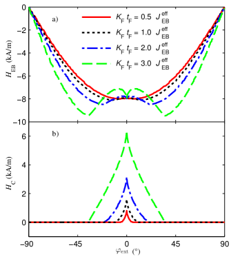
Figure 4: (a) $H_{\mathrm{EB}}$ and (b) $H_{\mathrm{C}}$ as a function of angle calculated using equation (7) for different $K_{\mathrm{F}}$. Material parameters used for the UMA were $K_{\mathrm{F}}=500$ J/m³ (red line), $K_{\mathrm{F}}=1000$ J/m³ (black dotted), $K_{\mathrm{F}}=2000$ J/m³ (blue dash-dotted) and $K_{\mathrm{F}}=4000$ J/m³ (green dashed). Other material parameters can be found in table 1.

From figure 4 it is evident, that the magnetic anisotropy of the F not only increases $H_{\mathrm{C}}$, but also has a big influence on the shape of $H_{\mathrm{EB}}$ as a function of $\varphi_{\mathrm{ext}}$. This is in accordance to previous calculations Camarero et al. (2005); Bai et al. (2010), where the angular dependence of EB and coercive fields was calculated for the classical model of Meiklejohn and Bean without using a RMA term. The most prominent characteristics are the triangular shape of the coercivity with a broadened base for higher UMA of the F and the maximum of $H_{\mathrm{EB}}(\varphi_{\mathrm{ext}})$ shifting away from the magnetic easy axis with increased magnetic anisotropy in the F. The principle shape of both characteristics is solely defined by the strengths of the exchange anisotropy and the F anisotropy.
However, the influence of the second source of coercivity, i.e. the RMA, is different. From figure 5 it is obvious that the general shape of $H_{\mathrm{EB}}(\varphi_{\mathrm{ext}})$ is almost not altered by the relative strength of the RMA. The dependence of $H_{\mathrm{EB}}(\varphi_{\mathrm{ext}})$ on the strength of the RMA decreases for EB systems possessing smaller UMA and vanishes for systems without F anisotropy. The shape of the coercivity mediated by $E_{\mathrm{RMA}}$ in general is not triangular but Lorentzian-like. For systems, which have RMA and UMA, the shape of the coercivity in first order is a superposition of both contributions.

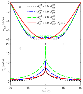
Figure 5: (a) $H_{\mathrm{EB}}$ and (b) $H_{\mathrm{C}}$ as a function of angle calculated using equation (7) for different $J_{\mathrm{C}}^{\mathrm{eff}}$. Material parameters used for the RMA were $J_{\mathrm{C}}^{\mathrm{eff}}=0.1$ mJ/m² (red line), $J_{\mathrm{C}}^{\mathrm{eff}}=0.05$ mJ/m² (black dotted), $J_{\mathrm{C}}^{\mathrm{eff}}=0.1$ mJ/m² (blue dash-dotted) and $J_{\mathrm{C}}^{\mathrm{eff}}=0.2$ mJ/m² (green dashed). For the UMA $K_{\mathrm{F}}=0$ J/m³ (red line) and $K_{\mathrm{F}}=2000$ J/m³ (others) was used. Other material parameters can be found in table 1.

From figure 6 it is evident, that $H_{\mathrm{EB}}$ and $H_{\mathrm{C}}(\varphi_{\mathrm{ext}})$ not only depend on the strength of the RMA but also on $\tau_{\mathrm{avg}}$. For an increased average relaxation time of the Class II grains the plateau of $H_{\mathrm{EB}}(\varphi_{\mathrm{ext}})$ close to the magnetic easy axis of the system flattens and the peak in $H_{\mathrm{C}}(\varphi_{\mathrm{ext}})$ becomes broader. For long $\tau_{\mathrm{avg}}$ the minimum of $H_{\mathrm{C}}(\varphi_{\mathrm{ext}})$ is increased leading to a non vanishing coercive field for $\varphi_{\mathrm{ext}}$ far away from the magnetic easy axis of the system.

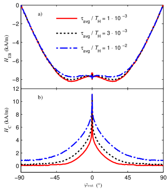
Figure 6: (a) $H_{\mathrm{EB}}$ and (b) $H_{\mathrm{C}}$ as a function of angle calculated using equation (7) for different $\tau_{\mathrm{avg}}$. Material parameters used for the RMA were $\tau_{\mathrm{avg}}/T_{\mathrm{H}}=10^{-3}$ (red line), $\tau_{\mathrm{avg}}/T_{\mathrm{H}}=3\cdot 10^{-2}$ (black dotted), $\tau_{\mathrm{avg}}/T_{\mathrm{H}}=1\cdot 10^{-2}$ (blue dash-dotted). Other material parameters can be found in table 1.

Looking at the angular dependencies of $H_{\mathrm{EB}}(\varphi_{\mathrm{ext}})$ and $H_{\mathrm{C}}(\varphi_{\mathrm{ext}})$, respectively, there is a clear difference in the influence of the two sources of coercivity. While $H_{\mathrm{EB}}(\varphi_{\mathrm{ext}})$ is strongly affected by the UMA, $H_{\mathrm{C}}(\varphi_{\mathrm{ext}})$ has different shapes for the two magnetic anisotropies mediating coercivity. Therefore, it is possible to determine the dominant magnetic anisotropy being responsible for the coercivity by measuring $H_{\mathrm{C}}$ as a function of $\varphi_{\mathrm{ext}}$.

IV.2 Comparison with experiment

The model was tested by comparing it to experimental data of $H_{\mathrm{EB}}(\varphi_{\mathrm{ext}})$ and $H_{\mathrm{C}}(\varphi_{\mathrm{ext}})$, obtained by vectorial magnetooptic Kerr magnetometry (figure 7). The experimentally determined relation of $H_{\mathrm{EB}}(\varphi_{\mathrm{ext}})$ is similar to one of the calculations of figure 4, indicating that the system possesses the assumed UMA (here with the magnetic easy axis at $\gamma_{\mathrm{F}}\approx 80^{\circ}$) of the Co₇₀Fe₃₀ layer. In contrast to the triangular shape of $H_{\mathrm{C}}(\varphi_{\mathrm{ext}})$ for the simulated system having UMA as the only source of coercivity, the experimentally detected shape of $H_{\mathrm{C}}(\varphi_{\mathrm{ext}})$ is curved. Therefore, elements of both coercivity mediating magnetic anisotropies are visible in the experiment.
Additionally, there is a Fano-like structureFano (1961) in $H_{\mathrm{EB}}(\varphi_{\mathrm{ext}})$ for measurements along the magnetic easy direction at an angle of about 80^∘ observable, which does not appear for the other magnetic easy direction around 260^∘ measured later. Such a curvature results, when $\gamma_{\mathrm{EB}}$ and $\gamma_{\mathrm{F}}$ are not aligned parallelJiménez et al. (2011), which is a result of a misalignment between the external magnetic fields during sample deposition and field cooling. In the present case this misalignment is very small and vanishes during the measurement. This may be connected to training effects, especially because it is well known that thermal activation can change the direction of EBvan der Heijden et al. (1998).

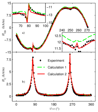
Figure 7: (a) $H_{\mathrm{EB}}$ and (b) $H_{\mathrm{C}}$  as a function of angle (black symbols) of a system of Cu${}^{50~{}\mathrm{nm}}$/Ir₁₇Mn₈₃${}^{30~{}\mathrm{nm}}$/Co₇₀Fe₃₀${}^{15~{}\mathrm{nm}}$/Si${}^{20~{}\mathrm{nm}}$. The dashed line (green) corresponds to numerical calculations based on equation (7) using a resolution of 0.5^∘ for $\beta_{\mathrm{F}}$. Material parameters used can be found in table 2. The red line corresponds to a numerical calculation based on equation (8) using the same parameters. For $H_{\mathrm{C}}$ there is almost no difference for both calculations.

A fit of the material properties by the model in equation 7 to the experimental data yields a numerically calculated dependency of $H_{\mathrm{EB}}(\varphi_{\mathrm{ext}})$ and $H_{\mathrm{C}}(\varphi_{\mathrm{ext}})$, which agrees almost perfectly with the experimental values (green line in figure 7). The normalized root-mean-square deviation $\sigma$ as a matching factor yields $\sigma_{\mathrm{EB}}=2.4~{}\%$ for the EB and $\sigma_{\mathrm{C}}=3.6~{}\%$ for the coercive field relation. Due to the change of $\gamma_{\mathrm{EB}}$ indicated by the curvature, different values for $\gamma_{\mathrm{EB}}$ where assumed for $\varphi_{\mathrm{ext}}<180^{\circ}$ and $\varphi_{\mathrm{ext}}>180^{\circ}$.
The calculated values for $H_{\mathrm{EB}}(\varphi_{\mathrm{ext}})$, however, are slightly bigger, because the absolute values in the experiment are not equal for the positive and the negative part of the relation. The discrepancy is not connected to the thermal training effect Schlenker (1968); Binek (2004), because the difference is reproducible in repetitive measurements. We, therefore, connect this phenomenon with the measurement procedure: Before each magnetization curve is recorded a calibration of the detector system was performed, allowing a larger number of AF grains to relax into the energetic state favored by the apparent magnetization direction. Therefore, the number of grains which contribute to the magnetization curve shift is increased (decreased), when the apparent magnetization direction of the F is parallel (antiparallel) to the magnetic easy direction of the unidirectional magnetic anisotropy. This effect can be accounted for by an additional magnetic anisotropy term $E_{\mathrm{add}}$, which energetically favors the direction of the initial magnetic field $\varphi_{\mathrm{ini}}$ of each magnetization curve leading to the total energy density

$$E_{2}=E_{1}+E_{\mathrm{add}},~{}\mathrm{with}~{}E_{\mathrm{add}}=-J_{\mathrm{eff}}^{\mathrm{add}}\cos{\left(\beta_{\mathrm{F}}-\varphi_{\mathrm{ini}}\right)}$$ (8)

Here, $J_{\mathrm{add}}^{\mathrm{eff}}$ is the effective exchange interaction connected to the additional grains relaxing at the beginning of each magnetization curve. Using equation (8) for the calculation (red line in figure 7), a very small value for $J_{\mathrm{add}}^{\mathrm{eff}}$ reduces the deviations further to $\sigma_{\mathrm{EB}}=1.9\%$ and $\sigma_{\mathrm{C}}=3.6\%$.

Table 2: Material constants obtained by fitting the numerical calculations to the experimental data in figure 7. The error corresponds to the uncertainty in the fit constants introduced by a variation of the starting conditions by a factor of 3.

Material Constant	Used value
$K_{\mathrm{F}}$	$(3300\pm 300)$ J/m3
$t_{\mathrm{F}}$	15 nm
$M_{\mathrm{sat}}$	1230 kA/m
$J_{\mathrm{EB}}^{\mathrm{eff}}$	$(0.285\pm 0.03)$ mJ/m2
$J_{\mathrm{C}}^{\mathrm{eff}}$	$(0.15\pm 0.2)$ mJ/m2
$J_{\mathrm{add}}^{\mathrm{eff}}$	$(0.011\pm 0.002)$ mJ/m2 ,
$\tau_{\mathrm{avg}}$	$(300\pm 100)$ ms
$\gamma_{\mathrm{EB}}-\gamma_{\mathrm{F}}(\varphi_{\mathrm{ext}}<180^{\circ})$	$(2.5\pm 1)$∘ ,
$\gamma_{\mathrm{EB}}-\gamma_{\mathrm{F}}(\varphi_{\mathrm{ext}}>180^{\circ})$	$(0\pm 1)$∘ ,

It is possible to use the model for revealing the important magnetic material properties of EB layer systems including effects related to the micro magnetic fine structure of the AF. We believe the error of most of the received material properties to be smaller than 10 %, because even strong variations in the starting conditions of the fit by a factor of 3 results in almost the same material constants. Especially $J_{\mathrm{EB}}^{\mathrm{eff}}$ and the misalignment between $\gamma_{\mathrm{EB}}$ and $\gamma_{\mathrm{F}}$ can be detected with great precision. The calculations are not so sensitive on $\tau_{\mathrm{avg}}$, where the uncertainty is about 30 %. This is not unexpected, because the relaxation times of the individual AF grains differ by several orders of magnitude Fulcomer and Charap (1972); Ehresmann et al. (2005).

IV.3 Influence of the measurement time

The proposed model and its precursors strongly focus on the impact of the relaxation times of the individual AF grains.Fulcomer and Charap (1972); Ehresmann et al. (2005); O’Grady et al. (2010) Thus, it is very important to take care of the experimental timescales, because they define how to classify the AF grains into the four different categories, i.e. the position of the borderlines in figure 1. To show the impact of the experimental timescales and to verify our approach on how to design the RMA, $H_{\mathrm{EB}}(\varphi_{\mathrm{ext}})$ and $H_{\mathrm{C}}(\varphi_{\mathrm{ext}})$ were measured in dependence of $T_{\mathrm{H}}$. The impact of the available timescales on this relations is undeniably small as depicted in figure 8.

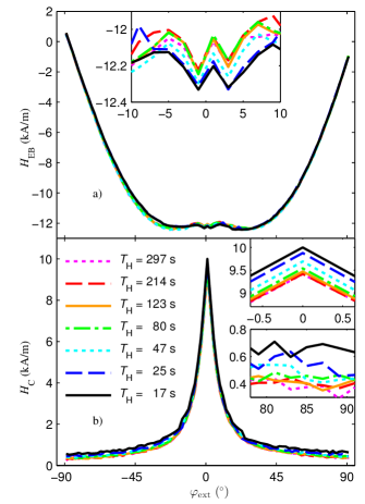
Figure 8: (a) $H_{\mathrm{EB}}$ and (b) $H_{\mathrm{C}}$  as a function of angle of a system of Cu${}^{50~{}\mathrm{nm}}$/Ir₁₇Mn₈₃${}^{30~{}\mathrm{nm}}$/Co₇₀Fe₃₀${}^{15~{}\mathrm{nm}}$/Si${}^{20~{}\mathrm{nm}}$ for different measurement times of the magnetization curves $T_{\mathrm{H}}$.

Nevertheless, it is possible to see the impact of the measurement time by looking at the extreme values. The impact of the measurement time is similar to the impact of temperature in general as the underlying mechanisms can be described by the Néel-Arrhenius law. Therefore, we do not want to focus on the behavior of the absolute maximum values of $H_{\mathrm{EB}}$ and $H_{\mathrm{C}}$, which were discussed several times before and are well described by the polycrystalline model.Fulcomer and Charap (1972); O’Grady et al. (2010) The situation is different for the minimal values $H_{\mathrm{C,min}}$ of the relation $H_{\mathrm{C}}(\varphi_{\mathrm{ext}})$ (see figure 9), which correspond to the heavy axis magnetization curves.

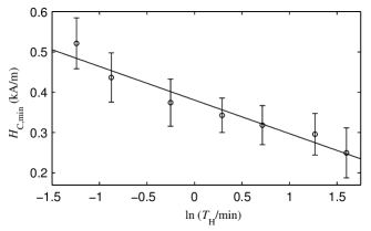
Figure 9: Minimum of the relation $H_{\mathrm{C}}(\varphi_{\mathrm{ext}})$ for different $T_{\mathrm{H}}$. The error corresponds to the uncertainty in the determination of $H_{\mathrm{C}}$. The line is a linear fit serving as a guide to the eye.

In first order $H_{\mathrm{C,min}}$ as a function of $T_{\mathrm{H}}$ shows a logarithmic decrease (linear decrease in the logarithmic presentation). In the calculations in figure 6 it was shown that $H_{\mathrm{C,min}}$ is nonzero if a RMA is used under consideration of the average relaxation time of the Class II grains. Further, $H_{\mathrm{C,min}}$ was increased for higher fractions of $\tau_{\mathrm{avg}}$/$T_{\mathrm{H}}$. Despite the fact that $\tau_{\mathrm{avg}}$ should strongly depend on $T_{\mathrm{H}}$ because changing the timescale dramatically changes the thermal stability of the AF grains, it is very reasonable that the fraction $\tau_{\mathrm{avg}}$/$T_{\mathrm{H}}$ is decreased for longer $T_{\mathrm{H}}$. Thus, the increase of $H_{\mathrm{C,min}}$ for faster measurements is expected by theory and, therefore, is another argument for the validity of the proposed model.

V Conclusion

In this study, we have shown a model based on the concepts of Stoner and Wohlfarth, which allows numerical calculations of $H_{\mathrm{EB}}$ and $H_{\mathrm{C}}$  in dependence of the external magnetic field angle including the thermal instabilities of the polycrystalline AF layer in a fast and simple approach. We were able to show, that the two main sources of coercivity, namely the F magnetic anisotropy and the RMA resulting from the exchange interaction of thermally unstable grains, can be disentangled via the angular dependency of $H_{\mathrm{EB}}$ and $H_{\mathrm{C}}$. Adjusting the calculations to the experimental data shows excellent agreement. For a Si/Cu${}^{50~{}\mathrm{nm}}$/Ir₁₇Mn₈₃${}^{30~{}\mathrm{nm}}$/Co₇₀Fe₃₀${}^{15~{}\mathrm{nm}}$/Si${}^{20~{}\mathrm{nm}}$ system F magnetic anisotropy with $K_{\mathrm{F}}=(3300\pm 300)~{}\mathrm{J~{}m^{-3}}$ and uniaxial anisotropy with $J_{\mathrm{EB}}^{\mathrm{eff}}=(0.285\pm 0.03)~{}\mathrm{J~{}m^{-2}}$ was determined. For the RMA an energy density of $J_{\mathrm{C}}^{\mathrm{eff}}=(0.15\pm 0.2)~{}\mathrm{J~{}m^{-2}}$ and an average relaxation time of $\tau_{\mathrm{avg}}=(300\pm 100)~{}\mathrm{ms}$ was found. Further, we were able to prove our model as it predicts the evolution of $H_{\mathrm{EB}}(\varphi_{\mathrm{ext}})$ and $H_{\mathrm{C}}(\varphi_{\mathrm{ext}})$ when the measurements are performed on different time scales.
We suggest using this technique for sample characterizations, for example to study the influence of ion bombardment on EB samples, when a complete characterization of a sample including its grain size distribution and temperature dependency is too intricate.

VI Acknowledgments

NDM thanks the University of Kassel for the Universität Kassel Promotionsstipendium.

References

- Meiklejohn and Bean (1956) W. H. Meiklejohn and C. P. Bean, Phys. Rev. 102, 1413 (1956).
- Meiklejohn and Bean (1957) W. H. Meiklejohn and C. P. Bean, Phys. Rev. 105, 904 (1957).
- Geshev et al. (2002) J. Geshev, L. G. Pereira, and J. E. Schmidt, Phys. Rev. B 66, 134432 (2002).
- Kim et al. (2003) J. Kim, S. Kim, K. Lee, B. Kim, J. Kim, S. Lee, D. Hwang, C. Kim, and C. Kim, J. Appl. Phys. 93, 7714 (2003).
- Radu and Zabel (2008) F. Radu and H. Zabel, in Magnetic heterostructures (Springer, 2008) p. 97.
- Nogu s and Schuller (1999) J. Nogu s and I. K. Schuller, J. Magn. Magn. Mater 192, 203 (1999).
- Ehresmann et al. (2015) A. Ehresmann, I. Koch, and D. Holzinger, Sensors 15, 28854 (2015).
- Ehresmann et al. (2006) A. Ehresmann, D. Engel, T. Weis, A. Schindler, D. Junk, J. Schmalhorst, V. Höink, M. Sacher, and G. Reiss, Phys. Status Solidi (b) 243, 29 (2006).
- Ehresmann et al. (2011a) A. Ehresmann, D. Lengemann, T. Weis, A. Albrecht, J. Langfahl-Klabes, F. Göllner, and D. Engel, Adv. Mater. 23, 5568 (2011a).
- Holzinger et al. (2015) D. Holzinger, I. Koch, S. Burgard, and A. Ehresmann, ACS Nano 9, 7323 (2015).
- O’Grady et al. (2010) K. O’Grady, L. Fernandez-Outon, and G. Vallejo-Fernandez, J. Magn. Magn. Mater 322, 883 (2010).
- Soeya et al. (1996) S. Soeya, M. Fuyama, S. Tadokoro, and T. Imagawa, J. Appl. Phys. 79, 1604 (1996).
- Ehresmann et al. (2005) A. Ehresmann, D. Junk, D. Engel, A. Paetzold, and K. Röll, J. Phys. D: Appl. Phys. 38, 801 (2005).
- Fulcomer and Charap (1972) E. Fulcomer and S. H. Charap, J. Appl. Phys. 43, 4190 (1972).
- Vallejo-Fernandez et al. (2010) G. Vallejo-Fernandez, N. Aley, J. Chapman, and K. O’Grady, Appl. Phys. Lett. 97, 2505 (2010).
- Vallejo-Fernandez et al. (2008) G. Vallejo-Fernandez, L. Fernandez-Outon, and K. O’Grady, J. Phys. D: Appl. Phys. 41, 112001 (2008).
- Ehresmann et al. (2011b) A. Ehresmann, C. Schmidt, T. Weis, and D. Engel, J. Appl. Phys. 109, 023910 (2011b).
- Engel et al. (2005) D. Engel, A. Ehresmann, J. Schmalhorst, M. Sacher, V. Höink, and G. Reiss, J. Magn. Magn. Mater 293, 849 (2005).
- Harres and Geshev (2012) A. Harres and J. Geshev, J. Phys.: Condens. Matter 24, 326004 (2012).
- Camarero et al. (2005) J. Camarero, J. Sort, A. Hoffmann, J. M. García-Martín, B. Dieny, R. Miranda, and J. Nogués, Phys. Rev. Lett. 95, 057204 (2005).
- Ambrose et al. (1997) T. Ambrose, R. Sommer, and C. Chien, Phys. Rev. B 56, 83 (1997).
- Hoffmann et al. (2003) A. Hoffmann, M. Grimsditch, J. Pearson, J. Nogués, W. Macedo, and I. K. Schuller, Phys. Rev. B 67, 220406 (2003).
- Stoner and Wohlfarth (1947) E. C. Stoner and E. Wohlfarth, Nature 160, 650 (1947).
- Stoner and Wohlfarth (1948) E. C. Stoner and E. P. Wohlfarth, Phil. Trans. R. Soc. Lond. 240, 599 (1948).
- Jiménez et al. (2009) E. Jiménez, J. Camarero, J. Sort, J. Nogués, A. Hoffmann, F. Teran, P. Perna, J. M. García-Martín, B. Dieny, and R. Miranda, Appl. Phys. Lett. 95, 122508 (2009).
- Aley et al. (2008) N. Aley, G. Vallejo-Fernandez, R. Kroeger, B. Lafferty, J. Agnew, Y. Lu, and K. O’Grady, IEEE Trans. Magn. 44, 2820 (2008).
- Nakamura et al. (1985) K. Nakamura, T. Asaka, S. Asari, Y. Ota, and A. Itoh, IEEE Trans. Magn. 21, 1654 (1985).
- Kuschel et al. (2011) T. Kuschel, H. Bardenhagen, H. Wilkens, R. Schubert, J. Hamrle, J. Pištora, and J. Wollschläger, J. Phys. D: Appl. Phys. 44, 265003 (2011).
- Hubert and Schäfer (1998) A. Hubert and R. Schäfer, Magnetic domains: the analysis of magnetic microstructures (Springer, 1998).
- Vavassori (2000) P. Vavassori, Appl. Phys. Lett. 77, 1605 (2000).
- McCord et al. (2003) J. McCord, R. Schäfer, R. Mattheis, and K.-U. Barholz, J. Appl. Phys. 93, 5491 (2003).
- Nieber and Kronmüller (1991) S. Nieber and H. Kronmüller, Phys. Status Solidi (b) 165, 503 (1991).
- Kim et al. (2006) D. Y. Kim, C. Kim, C.-O. Kim, M. Tsunoda, and M. Takahashi, J. Magn. Magn. Mater 304, 56 (2006).
- Öksüzoğlu et al. (2011) R. M. Öksüzoğlu, M. Yıldırım, H. Çınar, E. Hildebrandt, and L. Alff, J. Magn. Magn. Mater 323, 1827 (2011).
- Kuschel et al. (2012) T. Kuschel, J. Hamrle, J. Pištora, K. Saito, S. Bosu, Y. Sakuraba, K. Takanashi, and J. Wollschläger, J. Phys. D: Appl. Phys. 45, 495002 (2012).
- Steenbeck et al. (2004) K. Steenbeck, R. Mattheis, and M. Diegel, J. Magn. Magn. Mater 279, 317 (2004).
- Stiles and McMichael (1998) M. Stiles and R. D. McMichael, Phys. Rev. B 59, 3722 (1998).
- Bai et al. (2010) Y. Bai, G. Yun, and N. Bai, J. Appl. Phys. 107, 033905 (2010).
- Fano (1961) U. Fano, Phys. Rev. 124, 1866 (1961).
- Jiménez et al. (2011) E. Jiménez, J. Camarero, P. Perna, N. Mikuszeit, F. Terán, J. Sort, J. Nogués, J. M. García-Martín, A. Hoffmann, B. Dieny, et al., J. Appl. Phys. 109, 07D730 (2011).
- van der Heijden et al. (1998) P. A. A. van der Heijden, T. F. M. M. Maas, W. J. M. de Jonge, J. C. S. Kools, F. Roozeboom, and P. J. van der Zaag, Appl. Phys. Lett. 72, 492 (1998).
- Schlenker (1968) C. Schlenker, Phys. Status Solidi (b) 28, 507 (1968).
- Binek (2004) C. Binek, Phys. Rev. B 70, 014421 (2004).