Bell’s Inequalities for Continuous-Variable Systems in Generic Squeezed States

Abstract

Bell’s inequality for continuous-variable bipartite systems is studied. The inequality is expressed in terms of pseudo-spin operators and quantum expectation values are calculated for generic two-mode squeezed states characterized by a squeezing parameter $r$ and a squeezing angle $\varphi$. Allowing for generic values of the squeezing angle is especially relevant when $\varphi$ is not under experimental control, such as in cosmic inflation, where small quantum fluctuations in the early Universe are responsible for structures formation. Compared to previous studies restricted to $\varphi=0$ and to a fixed orientation of the pseudo-spin operators, allowing for $\varphi\neq 0$ and optimizing the angular configuration leads to a completely new and rich phenomenology. Two dual schemes of approximation are designed that allow for comprehensive exploration of the squeezing parameters space. In particular, it is found that Bell’s inequality can be violated when the squeezing parameter $r$ is large enough, $r\gtrsim 1.12$, and the squeezing angle $\varphi$ is small enough, $\varphi\lesssim 0.34\,e^{-r}$.

I Introduction

Bell’s inequalities Bell (1964) play a major role in Physics. Their experimental violation Aspect et al. (1982a, b); Weihs et al. (1998); Hensen et al. (2015) demonstrates that Nature cannot be described by a strongly local (no causal influence travels faster than light) and deterministic theory. Instead, it obeys the laws of Quantum Mechanics, where a violation can occur when the system is placed in an entangled state. Historically, this type of quantum states was considered for the first time by Einstein, Podolsky and Rosen (EPR) in LABEL:Einstein:1935rr. In that paper, they studied a system made of two particles with a quantum state entangled in position space. Subsequent works have rather formulated the problem in terms of discrete variables, typically spin variables for which the Bell inequalities usually takes the Clauser-Horne-Shimony-Holt (CHSH) form Clauser et al. (1969). Recently, however, in Ref. Larsson (2004), it was shown how (discrete) pseudo-spin operators can be constructed out of (continuous) position operators, thus opening the possibility to test the Bell inequalities in its CHSH form for continuous variable systems.

Testing Bell’s inequalities for continuous variable systems Chen et al. (2002); Yarnall et al. (2007); Larsson (2003); Brukner et al. (2003); Dorantes and Lucio M (2009) is interesting not only for investigating the EPR argument in its original formulation but also because it allows us to treat the case of quantum fields where the role of the continuous variable is played by the (Fourier) amplitude of the field. This is especially relevant because when a quantum field interacts with a classical source, particle creation occurs and, typically, the corresponding system is in a squeezed state, an example of entangled state. Such states contains genuine quantum correlations as can also be checked by computing their quantum discord Henderson and Vedral (2001); Ollivier and Zurek (2001); Martin and Vennin (2016a). The above mentioned situation arises, for instance, in the Schwinger effect Schwinger (1951) but also in the cosmic inflationary mechanism Starobinsky (1979, 1980); Sato (1981); Guth (1981); Linde (1982); Mukhanov and Chibisov (1981); Albrecht and Steinhardt (1982); Hawking (1982); Starobinsky (1982); Guth and Pi (1982); Bardeen et al. (1983); Linde (1983) (for reviews, see Refs. Martin (2005a, b, 2004, 2013); Vennin et al. (2015); Martin (2015)) for large scale structures growth and Cosmic Microwave Background Radiation (CMBR) anisotropies Grishchuk and Sidorov (1990); Martin (2008).

In this paper, we reconsider the work of Ref. Larsson (2004) and extend it in various directions, in order to be able to treat the case of quantum field theory and cosmology, topics that we plan to address in subsequent papers Martin and Vennin (2016b). Compared to Ref. Larsson (2004), we have obtained several new and important results that we now briefly describe. Firstly, we have treated the general case of a two-mode squeezed state with non-vanishing squeezing angle. In LABEL:2004PhRvA..70b2102L, the squeezing angle was set to zero since it is a controllable parameter in the laboratory and, hence, might be tuned to zero by working with specific experimental set-ups. However, in the case of e.g. cosmic inflation, the squeezing angle is “God-given” and, crucially, is non-vanishing and dynamical Martin et al. (2012); Martin (2012). This leads to a new and rich phenomenology. Secondly, we have numerically computed the pseudo-spin correlation functions and checked, when possible, our results with those of Ref. Larsson (2004). Global agreement is usually found even if we have also detected some slight differences. Thirdly, we have derived the optimal configuration leading to Bell’s inequality violation and have shown that very relevant differences can happen compared to the standard configuration used in Ref. Larsson (2004). For instance, we have exhibited squeezing parameters and angles such that a violation occurs for the optimal configuration but not for the standard one. Fourthly, we have obtained several approximated formulas regarding the pseudo-spin correlation functions and Bell’s operator expectation values which allowed us to better understand their dependence on the squeezing parameter and angle, and to interpret the numerical calculations. This also made possible studying violation of Bell’s inequality in regimes that would be impossible to reach numerically. Finally, for the first time to our knowledge, we have produced a map in the two-dimensional squeezing space (squeezing parameter and angle) of Bell’s inequality violation, see Fig. 5. This can serve as a useful guide to find the optimal squeezing parameter and angle given a specific experimental design.

The paper is organized as follows. In the next section, Sec. II, we introduce the pseudo-spin operators and study their properties. In Sec. III, we define the Bell operator and compute its expectation value for a two-mode squeezed state with arbitrary squeezing parameter and angle. We also pay special attention to the four angles involved in the definition of the Bell operator and derive the corresponding optimal configuration. In Sec. IV, we then investigate for which value of the squeezing parameter and angle Bell’s inequality is violated. Finally, in Sec. V, we present our conclusions. The technical aspects of the work are summarized in six appendices. In Sec. A, we numerically calculate the spin correlation functions. In Secs. B and C, we design generic approximation schemes allowing us to interpret the numerical computations and explore regions that cannot be accessed numerically. In Secs. D and E, we work out the large squeezing limit in the two dual cases where the squeezing angle is close to $0$ and $\pi/2$ respectively. In Sec. F finally, we show how different orientations of the pseudo-spin operators in phase space can be dealt with.

II Spin Operators for Continuous Variable Systems

The standard formulation of the Bell-CHSH inequality is written in term of spin variables. In this section, following LABEL:2004PhRvA..70b2102L, we explain how, in the case of a continuous variable system, one can define such quantities.

Let $Q$ be some continuous variable taking values in $\mathbb{R}$. It can be the position of a particle but also the (Fourier) amplitude of some quantum field. We divide the real axis in an infinite number of intervals $\left[n\ell,(n+1)\ell\right]$ of length $\ell$, where $n$ is an integer number running from $-\infty$ to $+\infty$. Then, we define the operator $\hat{P}(n,\ell)$ by

$$\hat{P}(n,\ell)\equiv\int_{n\ell}^{(n+1)\ell}{\rm d}Q\left|Q\rangle\langle Q\right|.$$ (1)

Clearly, $\hat{P}(n,\ell)$ is a projector since we have $\hat{P}(n,\ell)\hat{P}(m,\ell)=\delta_{nm}\hat{P}(n,\ell)$. Its eigenvectors can be written as (up to normalization) $\left[\hat{\mathbb{I}}-\hat{P}(n,\ell)\right]|\Psi\rangle$ and $\hat{P}(n,\ell)|\Psi\rangle$, where $|\Psi\rangle$ is any wavefunction, with corresponding eigenvalues $0$ and $1$ respectively. If one starts from a state $|\Psi\rangle$ which has support everywhere on $\mathbb{R}$, then the state $\hat{P}(n,\ell)|\Psi\rangle$ has support only in the interval $\left[n\ell,(n+1)\ell\right]$ and vanishes elsewhere. In some sense, it only retains the part of $|\Psi\rangle$ present in that interval. Moreover, the mean value of $\hat{P}(n,\ell)$ in the state $|\Psi\rangle$ gives the probability to find the system in the interval $\left[n\ell,(n+1)\ell\right]$.

The next step consists in introducing the following operator

$$\hat{S}_{z}(\ell) =\sum_{n=-\infty}^{+\infty}(-1)^{n}\hat{P}(n,\ell)$$ (2)

$$=\sum_{n=-\infty}^{\infty}(-1)^{n}\int_{n\ell}^{(n+1)\ell}{\rm d}Q|Q\rangle\langle Q|\,.$$ (3)

This defines a spin variable because the eigenvalues of this operator are $\pm 1$. This can be proven by noticing that $\hat{S}_{z}^{2}(\ell)=\hat{\mathbb{I}}$. Indeed, one has

$$\hat{S}_{z}^{2}(\ell) =\sum_{n=-\infty}^{+\infty}\sum_{m=-\infty}^{+\infty}(-1)^{n+m}$$

$$\times\int_{n\ell}^{(n+1)\ell}\int_{m\ell}^{(m+1)\ell}{\rm d}Q{\rm d}\overline{Q}\left|Q\rangle\langle Q\right|\overline{Q}\rangle\langle\overline{Q}|.$$ (4)

The scalar product $\langle Q|\overline{Q}\rangle$ gives a Dirac function $\delta(Q-\overline{Q})$ but only if $Q$ and $\overline{Q}$ belong to the same interval (otherwise they cannot be equal). This means that one must have $n=m$. As a consequence,

$$\hat{S}_{z}^{2}(\ell) =\sum_{n,m}(-1)^{n+m}\delta_{nm}\int_{n\ell}^{(n+1)\ell}{\rm d}Q\left|Q\rangle\langle Q\right|$$ (5)

$$=\sum_{n=-\infty}^{+\infty}\int_{n\ell}^{(n+1)\ell}{\rm d}Q\left|Q\rangle\langle Q\right|=\hat{\mathbb{I}},$$ (6)

since the probability to find the particle somewhere on the real axis is always one. The eigenvectors of $\hat{S}_{z}(\ell)$ are the wavefunctions having support within $\cup_{n}[2n\ell,(2n+1)\ell]$ (eigenvalue $+1$) and within $\cup_{n}[(2n-1)\ell,2n\ell]$ (eigenvalue $-1$). In particular, $\hat{P}(n,\ell)|\Psi\rangle$ is an eigenvector of $\hat{S}_{z}(\ell)$ with eigenvalue $(-1)^{n}$.

Having defined the spin operator along the $z$-axis, we now need to introduce the operators $\hat{S}_{x}(\ell)$ and $\hat{S}_{y}(\ell)$. To do this, we define an operator $\hat{T}(n,\ell)$ by the following expression

$$\hat{T}(n,\ell)=\int_{n\ell}^{(n+1)\ell}{\rm d}Q\left|Q\rangle\langle Q+\ell\right|.$$ (7)

Given the interval $\left[n\ell,(n+1)\ell\right]$, this operator takes the “translated” part (by $\ell$) of $|\Psi\rangle$ and restricts it to $\left[n\ell,(n+1)\ell\right]$. The fact that $\hat{T}(n,\ell)|\Psi\rangle$ has support only in this interval can be checked from the relation $\hat{P}(n,\ell)\hat{T}(n,\ell)=\hat{T}(n,\ell)$. In the same manner, one can show that the adjoint of $\hat{T}(n,\ell)$,

$$\hat{T}^{\dagger}(n,\ell)=\int_{n\ell+\ell}^{(n+2)\ell}{\rm d}Q\left|Q\rangle\langle Q-\ell\right|,$$ (8)

takes the translated part (by $-\ell$) of $|\Psi\rangle$ and restricts it to the interval $\left[(n+1)\ell,(n+2)\ell\right]$, as confirmed by the fact that $\hat{P}(n+1,\ell)\hat{T}^{\dagger}(n,\ell)=\hat{T}^{\dagger}(n,\ell)$.

One can then define the “spin step” operators $\hat{S}_{+}$ and $\hat{S}_{-}$ through the relations

$$\hat{S}_{+}(\ell)=\sum_{n=-\infty}^{\infty}\hat{T}(2n,\ell)=\sum_{n=-\infty}^{\infty}\int_{2n\ell}^{(2n+1)\ell}{\rm d}Q\left|Q\rangle\langle Q+\ell\right|$$ (9)

and $\hat{S}_{-}(\ell)=\hat{S}_{+}^{\dagger}(\ell)$. The operator $\hat{S}_{+}(\ell)$ takes an eigenstate of $\hat{S}_{z}(\ell)$ with eigenvalue $-1$ and transforms it into another eigenstate of $\hat{S}_{z}(\ell)$ but, this time, with eigenvalue $+1$. The proof goes as follows: an eigenstate of $\hat{S}_{z}(\ell)$ with eigenvalue $-1$ can be written as $\hat{P}(2n+1,\ell)|\Psi\rangle$. In order to check that $\hat{S}_{+}(\ell)\hat{P}(2n+1,\ell)|\Psi\rangle$ is also an eigenstate of $\hat{S}_{z}(\ell)$, one has to evaluate $\hat{S}_{z}(\ell)\hat{S}_{+}(\ell)\hat{P}(2n+1,\ell)|\Psi\rangle$. Using the relations $\hat{S}_{+}(\ell)\hat{P}(2n+1,\ell)=\hat{T}(2n,\ell)$ and $\hat{S}_{z}(\ell)\hat{T}(n,\ell)=(-1)^{n}\hat{T}(n,\ell)$, one obtains that $\hat{S}_{z}(\ell)\hat{S}_{+}(\ell)\hat{P}(2n+1,\ell)|\Psi\rangle=\hat{S}_{z}(\ell)\hat{T}(2n,\ell)|\Psi\rangle=(-1)^{2n}\hat{T}(2n,\ell)|\Psi\rangle=\hat{S}_{+}(\ell)\hat{P}(2n+1,\ell)|\Psi\rangle$, which demonstrates that, indeed, $\hat{S}_{+}(\ell)\hat{P}(2n+1,\ell)|\Psi\rangle$ is an eigenstate of $\hat{S}_{z}(\ell)$ with eigenvalue $+1$. A similar proof showing that $\hat{S}_{-}(\ell)$ takes an eigenstate of $\hat{S}_{z}(\ell)$ with eigenvalue $+1$ and transforms it into another eigenstate but with eigenvalue $-1$ can easily be constructed along the same lines.

One is now in a position to introduce the $x$ and $y$ components of the pseudo-spin system. They are defined in terms of the spin step operators by the usual expressions, namely

$$\hat{S}_{x}(\ell) =\hat{S}_{+}(\ell)+\hat{S}_{-}(\ell),$$ (10)

$$\hat{S}_{y}(\ell) =-i\left[\hat{S}_{+}(\ell)-\hat{S}_{-}(\ell)\right].$$ (11)

Using the result that $[\hat{S}_{z}(\ell),\hat{T}(n,\ell)]=2(-1)^{n}\hat{T}(n,\ell)$, one can verify that $[\hat{S}_{z}(\ell),\hat{S}_{x}(\ell)]=2i\hat{S}_{y}(\ell)$ and $[\hat{S}_{y}(\ell),\hat{S}_{z}(\ell)]=2i\hat{S}_{x}(\ell)$. Since one also has $[\hat{T}(2n,\ell),\hat{T}^{\dagger}(2m,\ell)]=\delta_{n,m}[\hat{P}(2n,\ell)-\hat{P}(2n+1,\ell)]$, one obtains $[\hat{S}_{x}(\ell),\hat{S}_{y}(\ell)]=2i[\hat{S}_{+}(\ell),\hat{S}_{-}(\ell)]=2i\hat{S}_{z}(\ell)$. Finally, one can check that $\hat{S}_{x}^{2}(\ell)=\hat{S}_{y}^{2}(\ell)=\hat{\mathbb{I}}$, which completes the construction of our spin operators. Notice that here, the choice of $\ell$ is entirely controllable by the observer.

III Bell’s Inequality

Having defined pseudo-spin operators in the last section, one can now proceed and introduce a Bell operator. Let us consider the case of a bipartite system $(1)\otimes(2)$. Since we want to study the Bell’s inequalities in their CHSH form, we define the following operator

$$\hat{B}(\ell) \equiv\left[{\bm{n}}\cdot\hat{{\bm{S}}}^{(1)}(\ell)\right]\otimes\left[{\bm{m}}\cdot\hat{{\bm{S}}}^{(2)}(\ell)\right]$$ (12)

$$+\left[{\bm{n}}\cdot\hat{{\bm{S}}}^{(1)}(\ell)\right]\otimes\left[{\bm{m}}^{\prime}\cdot\hat{{\bm{S}}}^{(2)}(\ell)\right]$$ (13)

$$+\left[{\bm{n}}^{\prime}\cdot\hat{{\bm{S}}}^{(1)}(\ell)\right]\otimes\left[{\bm{m}}\cdot\hat{{\bm{S}}}^{(2)}(\ell)\right]$$ (14)

$$-\left[{\bm{n}}^{\prime}\cdot\hat{{\bm{S}}}^{(1)}(\ell)\right]\otimes\left[{\bm{m}}^{\prime}\cdot\hat{{\bm{S}}}^{(2)}(\ell)\right],$$ (15)

where ${\bm{n}}$, ${\bm{n}}^{\prime}$, ${\bm{m}}$ and ${\bm{m}}^{\prime}$ are four arbitrary unit vectors that can be expanded in terms of their polar and azimuthal angles, ${\bm{n}}=\left(\sin\theta_{\bm{n}}\cos\phi_{\bm{n}},\sin\theta_{\bm{n}}\sin\phi_{\bm{n}},\cos\theta_{\bm{n}}\right)$ (and similar expressions for the three other vectors). From now on, without loss of generality, we set all azimuthal angles to zero. Let us then introduce the correlation function

$$E\left(\ell,{\bm{n}},{\bm{m}}\right)\equiv \left\langle\left[{\bm{n}}\cdot\hat{{\bm{S}}}^{(1)}(\ell)\right]\otimes\left[{\bm{m}}\cdot\hat{{\bm{S}}}^{(2)}(\ell)\right]\right\rangle$$ (16)

$$= \sin\theta_{\bm{n}}\sin\theta_{\bm{m}}\langle\hat{S}^{(1)}_{x}(\ell)\hat{S}^{(2)}_{x}(\ell)\rangle$$

$$+\cos\theta_{\bm{n}}\cos\theta_{\bm{m}}\langle\hat{S}^{(1)}_{z}(\ell)\hat{S}^{(2)}_{z}(\ell)\rangle\,,$$ (17)

where the expectation value is with respect to the quantum state of the system under scrutiny. In general, terms proportional to $\langle\hat{S}^{(1)}_{z}(\ell)\hat{S}^{(2)}_{x}(\ell)\rangle$ and $\langle\hat{S}^{(1)}_{x}(\ell)\hat{S}^{(2)}_{z}(\ell)\rangle$ are also present, but for the two-mode squeezed state we consider below, it is shown in Sec. A.4 that these correlators vanish. This expression allows us to calculate the expectation value of the Bell operator, namely

$$\langle\hat{B}(\ell)\rangle= E\left(\ell,\theta_{\bm{n}},\theta_{\bm{m}}\right)+E\left(\ell,\theta_{\bm{n}},\theta_{\bm{m}}^{\prime}\right)+E\left(\ell,\theta_{\bm{n}}^{\prime},\theta_{\bm{m}}\right)$$

$$-E\left(\ell,\theta_{\bm{n}}^{\prime},\theta_{\bm{m}}^{\prime}\right)\,.$$ (18)

Several remarks are in order here. Firstly, the correlation function does not involve the $y$-axis component of the spin and this is of course a consequence of the fact that we have taken vanishing azimuthal angles. Secondly, we notice that the expectation value of the Bell operator is entirely calculable in terms of the two-point correlation functions of the spin operators. This is the reason why we study them in detail in Sec. A. Thirdly, as is well-known, local realistic theories imply $|\langle\hat{B}(\ell)\rangle|\leq 2$ while quantum mechanics only imposes the so-called Cirel’son bound Cirel’Son (1980), namely $|\langle\hat{B}(\ell)\rangle|\leq 2\sqrt{2}$. Therefore, any situation such that $2<|\langle\hat{B}(\ell)\rangle|\leq 2\sqrt{2}$ will be referred to as violation of Bell’s inequalities.

Figure 1: Expectation value of the Bell operator $\hat{B}$ as a function of $\ell$, for different squeezing parameters $r$ and squeezing angle $\varphi=0$. Situations where $\langle\hat{B}\rangle>2$ indicate violation of Bell’s inequalities, and one can check that the Cirel’son bound $\langle\hat{B}\rangle<2\sqrt{2}$ is always satisfied.

Figure 2: Expectation value of the Bell operator $\hat{B}$ as a function of $\ell$, for $r=1$ (left panel) and $r=2$ (right panel), and different squeezing angles $\varphi$. As in Fig. 1, Bell’s inequality violation threshold $\langle\hat{B}\rangle=2$ and the Cirel’son bound $\langle\hat{B}\rangle<2\sqrt{2}$ are displayed, see the two horizontal black lines. One can see that, in general, increasing $\varphi$ from $0$ tends to make Bell’s inequalities violation more difficult to achieve. The situations where $\varphi=\pi/6$ and $\varphi=\pi/3$ give rise to exactly the same result (as a consequence of the invariance of $\langle\hat{B}\rangle$ under $\varphi\rightarrow\pi/2-\varphi$), which is why we have used a dashed line for $\varphi=\pi/3$.

Fourthly, the polar angles $\theta_{\bm{n}}$, $\theta_{\bm{m}}$, $\theta_{\bm{n}}^{\prime}$ and $\theta_{\bm{m}}^{\prime}$ need to be carefully chosen. The standard choice, made in LABEL:2004PhRvA..70b2102L, is to take $\theta_{\bm{n}}=0$, $\theta_{\bm{m}}=\pi/4$, $\theta_{\bm{n}}^{\prime}=\pi/2$ and $\theta_{\bm{m}}^{\prime}=-\pi/4$. However, this does not correspond to the optimal configuration. By varying Eq. (III) with respect to the four polar angles, one can show that the later is given by $\theta_{\bm{n}}=0$, $\theta_{\bm{n}}^{\prime}=\pi/2$ and $\theta_{\bm{m}}^{\prime}=-\theta_{\bm{m}}$ with

$$\theta_{\bm{m}}=\arctan\left[\frac{\langle\hat{S}^{(1)}_{x}(\ell)\hat{S}^{(2)}_{x}(\ell)\rangle}{\langle\hat{S}^{(1)}_{z}(\ell)\hat{S}^{(2)}_{z}(\ell)\rangle}\right].$$ (19)

In the following, we always work with this choice unless explicitly specified otherwise. With these angles, one has

$$\langle\hat{B}\rangle=2\sqrt{\langle\hat{S}^{(1)}_{z}(\ell)\hat{S}^{(2)}_{z}(\ell)\rangle^{2}+\langle\hat{S}^{(1)}_{x}(\ell)\hat{S}^{(2)}_{x}(\ell)\rangle^{2}}\,.$$ (20)

From this expression, the Cirel’son bound $\langle\hat{B}\rangle<2\sqrt{2}$ is easily obtained since the two-point correlators of the spin operators must be comprised between $-1$ and $1$ (having eigenvalues $-1$ and $1$).

In order to calculate concretely the expectation value of the Bell operator, see Eq. (III), we need to specify the quantum state in which the system is placed. In this paper, we consider the two-mode squeezed state

$$|\Psi_{2\,\mathrm{sq}}\rangle =\frac{1}{\cosh r}\sum_{n=0}^{\infty}e^{-2in\varphi}\tanh^{n}r|n_{1},n_{2}\rangle,$$ (21)

where $r>0$ is the squeezing parameter and $\varphi$ is the squeezing angle. So far only the case $\varphi=0$ was studied but, here, we treat the most general situation. The ket $|n_{1},n_{2}\rangle$ represents the state of the bipartite system such that the sub-systems $(1)$ and $(2)$ have the same number of quantas, namely $n$ (not to be confused with a situation where there would be $n_{1}$ quantas in the first system and $n_{2}$ quantas in the second one; in our notations, “$1$” and “$2$” are labels for the two sub-systems).

The quantum state (21) is exactly the state in which the cosmological fluctuations are placed at the end of inflation, see for instance Refs. Grishchuk and Sidorov (1990); Martin (2008). It is also worth noticing that, in this context, $r\simeq 100$, a much larger number than what can be achieved in the laboratory (typically a few). Since we have in mind applications to cosmology, this reinforces the motivation for deriving a large-squeezing limit as done in Sec. D. It is well-known that the CMBR is the best black body known in Nature Fixsen et al. (1996) since it is not possible to reproduce a thermal spectrum at this level of accuracy in the laboratory. In some sense, cosmological perturbations have a similar property, since they are placed in a quantum state the squeezing parameter of which is much larger than what can be obtained in the laboratory. As a final comment, let us also notice that, when $r$ goes to infinity, the state (21) exactly tends towards the EPR state.

It is also interesting to recall that the state (21) has a positive definite Wigner function Martin and Vennin (2016a). Bell suggested Bell (1987) that the non-negativity of the Wigner function, which can therefore be interpreted as a stochastic distribution, would prevent Bell’s inequality violation. However, in Refs. Gour et al. (2004); Revzen et al. (2005); Revzen (2006), it was shown that Bell’s inequalities violation can occur, in particular if the operators used are non-analytical in the dynamical variables, which is precisely the case of the pseudo-spin operators used in this work.

As mentioned before, calculating the expectation value of the Bell operator implies to evaluate the two-point correlation functions of the spin operators. Unfortunately, for the state (21), this cannot be done analytically and we have to rely on numerical calculations. The details of those computations are explained in Sec. A and, here, we just quote the results.

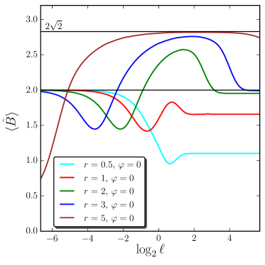
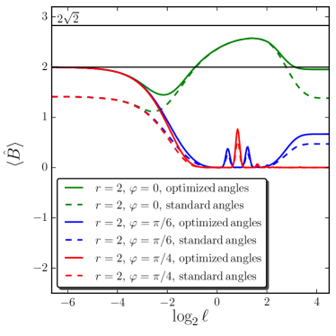
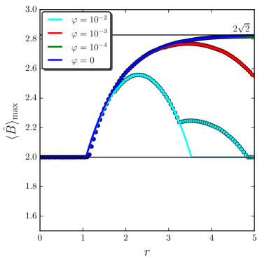
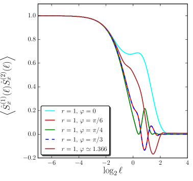
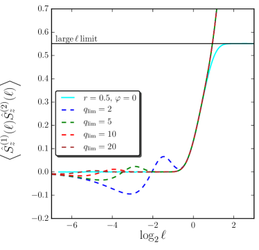
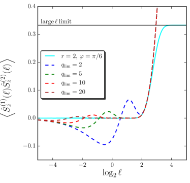
Let us first describe the case where the squeezing angle vanishes, see Fig. 1, where $\langle\hat{B}(\ell)\rangle$ is represented versus $\log_{2}\ell$ for different values of $r$. In the small $\ell$ limit, we have shown in Sec. B.2 that $\langle\hat{S}^{(1)}_{x}(\ell)\hat{S}^{(2)}_{x}(\ell)\rangle\rightarrow 1$ and $\langle\hat{S}^{(1)}_{y}(\ell)\hat{S}^{(2)}_{y}(\ell)\rangle=\langle\hat{S}^{(1)}_{z}(\ell)\hat{S}^{(2)}_{z}(\ell)\rangle\rightarrow 0$, hence $\langle\hat{B}(\ell)\rangle\rightarrow 2$ from Eq. (20) (in Fig. 1, this result is also valid for $r=5$ but, in that case, just happens for values of $\ell$ smaller than those plotted in the figure). In the large $\ell$ limit, we notice that we also have a plateau, the value of which depends on the squeezing parameter. It is shown in Sec. B.1 that, in this limit, $\langle\hat{S}^{(1)}_{x}(\ell)\hat{S}^{(2)}_{x}(\ell)\rangle=\langle\hat{S}^{(1)}_{y}(\ell)\hat{S}^{(2)}_{y}(\ell)\rangle\rightarrow 0$ and $\langle\hat{S}^{(1)}_{z}(\ell)\hat{S}^{(2)}_{z}(\ell)\rangle\rightarrow 2/\pi\arctan[\sinh(2r)]$, this last formula having already been obtained in LABEL:2004PhRvA..70b2102L. From Eq. (20), one then has

$$\langle\hat{B}(\ell)\rangle\rightarrow\frac{4}{\pi}\arctan\left[\sinh(2r)\right]$$ (22)

in this limit and one can check that this value fits very well the ones observed in the plot. Between the two plateaus, we observe a more complicated structure with a bump. In Sec. C, we develop an approximation scheme which is able to reproduce with very high accuracy the shape of this bump. Of course the most striking feature is that, for values such that $r\gtrsim 1.12$, one has violation of Bell’s inequality. One notices that, when $r$ becomes large, the Cirel’son bound is quickly saturated but never crossed, which further checks the consistency of our numerical computation. Let us also remark that the larger $r$, the wider the region where Bell’s inequality is violated.

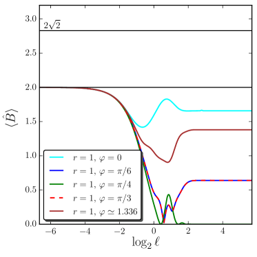
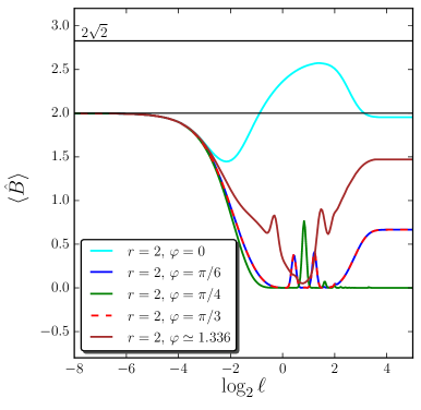
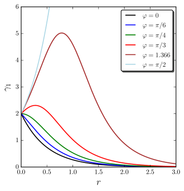
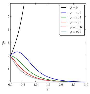
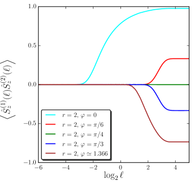
Let us now study the case of a non-vanishing squeezing angle. As already mentioned, this is the first time that this is done. The results are presented in Figs. 2 for $r=1$ and $\varphi=0$, $\pi/6$, $\pi/4$, $\pi/3$ and $1.366$ (left panel) and $r=2$ (right panel) for the same values of $\varphi$. As explained in Sec. A, the cases where $\varphi$ does not belong to $[0,\pi/4]$ can be easily deduced from the situations where $\varphi\in[0,\pi/4]$ applying straightforward transformation rules. In particular, it is shown that $\varphi$ and $\pi/2-\varphi$ give rise to the same expectation value of the Bell operator, and one can check that the curves for $\varphi=\pi/6$ and $\pi/3$ are indeed the same in Figs. 2.

Figure 3: Expectation value of the Bell operator $\hat{B}$ as a function of $\ell$, with the standard polar angles $\theta_{\bm{n}}=0$, $\theta_{\bm{m}}=\pi/4$, $\theta_{\bm{n}}^{\prime}=\pi/2$ and $\theta_{\bm{m}}^{\prime}=-\pi/4$ used in LABEL:2004PhRvA..70b2102L notably (dashed lines), and in the optimal configuration where $\theta_{\bm{n}}=0$, $\theta_{\bm{n}}^{\prime}=\pi/2$ and $\theta_{\bm{m}}^{\prime}=-\theta_{\bm{m}}$ is given by Eq. (19) (solid lines). The left panel presents the result for different values of $r$ and $\varphi=0$, while in the right panel, $r=2$ and different values of $\varphi$ are used.

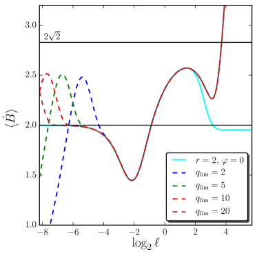
In the small $\ell$ limit, one still has the plateau at $\langle\hat{B}(\ell)\rangle\simeq 2$ in agreement with Sec. B.2 since this limit is independent of $\varphi$. In the large $\ell$ limit, a plateau is also present, the value of which depends this time both on $r$ and $\varphi$. In Sec. B.1, we shown that $\langle\hat{S}^{(1)}_{x}(\ell)\hat{S}^{(2)}_{x}(\ell)\rangle=\langle\hat{S}^{(1)}_{y}(\ell)\hat{S}^{(2)}_{y}(\ell)\rangle\rightarrow 0$ and that the limit of $\langle\hat{S}^{(1)}_{z}(\ell)\hat{S}^{(2)}_{z}(\ell)\rangle$ is given by Eq. (90). From Eq. (20), this gives rise to

$$\langle\hat{B}(\ell)\rangle {\rightarrow}\frac{4}{\pi}\arctan\left[\frac{\cos(2\varphi)\sinh(2r)}{\sqrt{\cosh^{2}(2r)-\cos^{2}(2\varphi)\sinh^{2}(2r)}}\right],$$ (23)

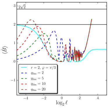
which directly generalizes Eq. (22). Between the two plateaus, one notices oscillatory patterns with various peaks and dips. This behavior is more complicated than for the case $\varphi=0$ where one just has a simple bump. But the most important difference between these configurations is of course that it seems more difficult to violate Bell’s inequalities when $\varphi\neq 0$. For instance, for $r=2$ and $\varphi=0$, there is a regime where $\langle\hat{B}(\ell)\rangle\geq 2$ while, for the other values of $\varphi\neq 0$ considered, this is not the case.

Figure 4: Expectation value of the Bell operator $\hat{B}$ as a function of $\ell$ for $r=3$ and $\varphi=0.03$, with the standard polar angles $\theta_{\bm{n}}=0$, $\theta_{\bm{m}}=\pi/4$, $\theta_{\bm{n}}^{\prime}=\pi/2$ and $\theta_{\bm{m}}^{\prime}=-\pi/4$ used in LABEL:2004PhRvA..70b2102L notably (dashed line), and in the optimal configuration where $\theta_{\bm{n}}=0$, $\theta_{\bm{n}}^{\prime}=\pi/2$ and $\theta_{\bm{m}}^{\prime}=-\theta_{\bm{m}}$ is given by Eq. (19) (solid line). Bell’s inequalities violation can be obtained in this state, but is detected only when working with the optimal angles.

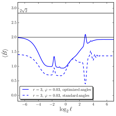
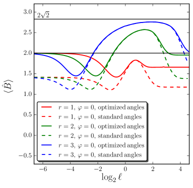
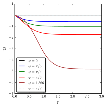
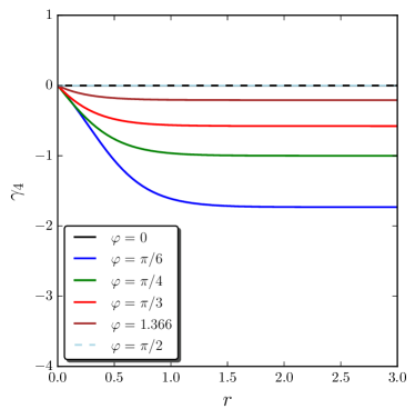
Finally, it is interesting to study the impact of working with optimized angles rather than with the standard choice, $\theta_{\bm{n}}=0$, $\theta_{\bm{m}}=\pi/4$, $\theta_{\bm{n}}^{\prime}=\pi/2$ and $\theta_{\bm{m}}^{\prime}=-\pi/4$. In Fig. 3, we have represented $\langle\hat{B}(\ell)\rangle$ for different values of $r$ and $\varphi=0$ (left panel) and $r=2$ and different values of $\varphi$ (right panel) in the cases of standard and optimized angles. One notices that, of course, the optimized result is always above the standard one. One also remarks that, although the two cases are similar in the vicinity of the bump, they strongly differ for the small and large $\ell$ plateaus. However, one could argue that working with optimized angles is, after all, not that important since around the region where Bell’s inequality is violated the standard angles approximately lead to the same result. But this is not always the case as revealed, for instance, in Fig. 4 where we have plotted $\langle\hat{B}(\ell)\rangle$ for $r=3$ and $\varphi=0.03$. We see that for the standard choice, no violation occurs while, for the optimized angles, the presence of a “feature” enables to cross the $\langle\hat{B}(\ell)\rangle=2$ threshold. Of course, this is only a specific case but, as a matter of fact, we have checked that it happens in many other situations.

IV Bell’s Inequality Violation in Squeezing Parameters Space

Figure 5: Maximum Bell’s operator expectation value $\langle\hat{B}\rangle_{\mathrm{max}}$ (where extremization has been performed over $\ell$ at the bump) as a function of the squeezing parameters $r$ and $\varphi$. The dashed white line stands for $\varphi\propto 0.34e^{-r}$, see Eq. (179), which delimits Bell’s inequality violation domain $\langle\hat{B}\rangle_{\mathrm{max}}>2$ in the large squeezing limit. The map is displayed for $\varphi\in[0,\pi/4]$ only, since any other value of $\varphi$ can be inferred from such configurations making use of Eqs. (71)-(73), and $r\in[0,5]$, since for larger values of $r$ the result is very accurately provided by Fig. 16.

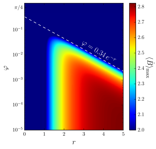
In the previous section, we have explicitly demonstrated that, for some values of $r$ and $\varphi$, the spin operators can lead to violation of Bell’s inequalities. The next obvious question is for which values of $r$ and $\varphi$ such a violation can be obtained. To answer it, in Fig. 5, we present a map of $\langle\hat{B}\rangle_{\mathrm{max}}$ in the $(r,\varphi)$ space. This map was obtained by constructing a grid of $300\times 300$ points in the $(r,\varphi)$ space and, for each value of $r$ and $\varphi$, determining the value of $\langle\hat{B}\rangle$ at the top of the bump (when this value was found to be smaller than $2$, we have put $\langle\hat{B}\rangle_{\mathrm{max}}=2$ since we know that, in the small $\ell$ limit, $\langle\hat{B}\rangle\rightarrow 2$).

Figure 6: Left panel: Expectation value of the Bell operator as a function of $\ell$ for $r=3$ and different values of $\varphi$. When $\varphi\neq 0$, on top of the usual bump, several features are present, that can lead to stronger Bell’s inequalities violation than in the bump only (see e.g. the case $r=3$ and $\varphi=0.015$ or $\varphi=0.02$). Right panel: Maximal expectation value of the Bell operator, where extremization has been performed over the bump making use of the approximation scheme developed in Sec. C (solid lines), and over the entire profile with the numerical results presented in Sec. A (circles). When a feature leads to stronger violation than the bump, as in the left panel for $r=3$ and $\varphi=0.015$ for instance, the two results are obviously different, otherwise the agreement is excellent.

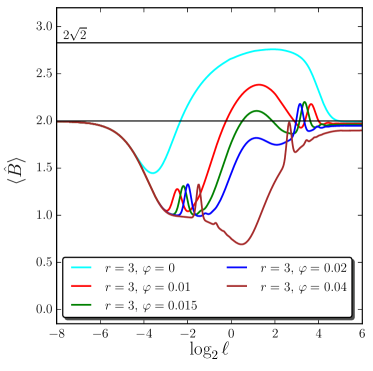
Exploring the squeezing parameter space can be, for some values of $r$ and $\varphi$, numerically very demanding. This is the reason why we have in fact determined the value of the Bell operator at the bump by means of the approximation developed in Sec. B. In that section, we have indeed shown that it always reproduces the bump very accurately. We have further checked that this method is efficient by comparing it with numerical results in the right panel of Fig. 6. In this plot, the solid lines correspond to the analytical approximation of Sec. B while the circles stand for the numerical results presented in Sec. A, where the maximum of $\langle\hat{B}\rangle$ is found in a given, sufficiently wide, range of $\log_{2}\ell$. For $\varphi=0$ for instance, they match very well and this validates our approach.

We notice, however, that for the case $\varphi=10^{-2}$ and $r\gtrsim 3.2$, the numerical method seems to predict results that strongly deviate from those obtained by means of the analytical approximation. The former clearly predicts $\langle\hat{B}\rangle_{\mathrm{max}}>2$ while the latter indicates that $\langle\hat{B}\rangle_{\mathrm{max}}=2$. This can be understood studying the left panel of Fig. 6 where we have represented $\langle\hat{B}\rangle$ for $r=3$ and $\varphi=0$, $0.01$, $0.015$, $0.02$ and $0.04$. For $\varphi=0$ and $\varphi=0.01$, we see that the maximum of $\langle\hat{B}\rangle$ is located at the bump. However, as soon as $\varphi\neq 0$, we notice the presence of features, i.e. secondary, smaller, bumps, located at smaller or larger values of $\log_{2}\ell$. For $\varphi\geq 0.015$, the first right feature actually corresponds to the maximum of $\langle\hat{B}\rangle$ which is, therefore, no longer given by the bump. For $\varphi=0.015$, the bump and this feature both correspond to situations where Bell’s inequality is violated but violation is stronger in the feature than in the bump. For $\varphi\geq 0.02$, Bell’s inequality is only violated at the feature and no longer at the bump. Clearly, when this happens, our analytical method breaks down and can no longer identify the maximum of $\langle\hat{B}\rangle$ over the full range of $\ell$. In this sense, the map in Fig. 5 only provides a sufficient, but not necessary, condition for violating Bell’s inequalities in the squeezing parameter space since only the maximal value of $\langle\hat{B}\rangle$ over the bump is displayed.

Let us now discuss the physical implications of the map given in Fig. 5. Firstly, in order to obtain violation of Bell’s inequalities, we see that there is a threshold in $r$, namely $r\gtrsim 1.12$. Of course, the larger $r$, the larger the violation. This is consistent with the fact Martin and Vennin (2016a) that the squeezing parameter $r$ measures the entanglement level of the state. Secondly, we notice that $\langle\hat{B}\rangle_{\mathrm{max}}$ decreases rapidly with $\varphi$. In other words, for a value of $r$ such that Bell’s inequality violation is obtained for $\varphi=0$, only very small non-vanishing squeezing angles still lead to violation. Moreover, the violation is always maximal for $\varphi=0$ and can only be less important for $\varphi\neq 0$. Thirdly, we clearly notice in Fig. 5 that the width of the $\varphi$ interval for which one has violation decreases with $r$. In fact, as shown in Sec. D, one can demonstrate that for sufficiently large $r$, $\langle\hat{B}\rangle_{\mathrm{max}}$ depends on $\varphi e^{r}$ only, and that Bell’s inequality violation occurs provided

$$\varphi<0.34e^{-r}.$$ (24)

This law is very important since it provides a simple criterion for Bell’s inequality violation in a regime (large squeezing) that cannot be reached numerically.

To summarize, Bell’s inequality violation is obtained if two conditions are met: firstly, $r$ must be large, quite an obvious conclusion indeed (and one notices that when $r\gtrsim 4$, the Cirel’son bound is completely saturated and there would be no point in going much further); secondly, $\varphi$ must be sufficiently small, and its fine-tuning close to $0$ increases with $r$ (in the most favorable case, namely close to the threshold $r\simeq 1.12$, one still must have $\varphi\lesssim 0.05$).

V Discussion and Conclusion

Let us now summarize our main results. Following the procedure of LABEL:2004PhRvA..70b2102L, we have introduced spin operators for continuous-variable systems, from which a Bell operator can be constructed. We have then calculated the expectation value of this Bell operator in a two-mode squeezed state, allowing for a non-vanishing squeezing angle $\varphi$.

This generalizes the previous results of LABEL:2004PhRvA..70b2102L in a direction that is necessary to follow if one wants to apply the present construction to situations where the role of the continuous variable is played by the (Fourier) amplitude of a quantum field, and where $\varphi$ is a non-vanishing quantity one does not have experimental control on. This is for instance the case of cosmic inflationary perturbations, which we plan to study in future publications Martin and Vennin (2016b). We have found that the observables involved in the present calculation are highly sensitive on $\varphi$ and that, compared to the situation $\varphi=0$, very different results can be obtained even for tiny, non-vanishing values of $\varphi$. Actually, if one needed to, this suggests that the spin operators discussed in this paper might provide a way to measure $\varphi$ very accurately. We have also optimized the polar angles defining the direction of the Bell operator, and showed that in some cases, this procedure is necessary to properly account for Bell’s inequalities violation.

Depending on the values of the squeezing parameters $r$ and $\varphi$, the numerical evaluation of the Bell operator expectation value can be numerically very expensive, if not impossible. For this reason, we have designed two dual schemes of approximation presented in Secs. A and E respectively, that allow one to explore the entire squeezing parameters space, and to gain some analytical insight on the results. In particular, a map of the maximal Bell’s operator expectation value was provided in Fig. 5, that can serve as a useful guide to find the optimal squeezing parameters values for a given experimental design. It was found that Bell’s inequalities violation occurs provided $r$ is sufficiently large and $\varphi$ sufficiently small. More precisely, it was shown that in the large squeezing limit, Bell’s inequalities violation is obtained if $\varphi\lesssim 0.34\,e^{-r}$.

At this stage, it is important to notice that although one does not necessarily have experimental control on $\varphi$, one is a priori free to choose the pseudo-spin operators with respect to another direction in phase space than the position $Q$ considered so far. In fact, in Sec. F, it is shown that if one performs a rotation in phase space with angle $\varphi$ and introduces $\overline{Q}_{i}=\cos\varphi\bar{Q}_{i}+\sin\varphi P_{i}$ and $\overline{P}_{i}=\cos\varphi P_{i}-\sin\varphi Q_{i}$, with $i=1,2$, then the squeezing angle of the resulting wavefunction $\Psi_{\rm 2\,sq}(\overline{Q}_{1},\overline{Q}_{2})$ vanishes. As a consequence, if one defines the pseudo-spin operators with respect to $\overline{Q}$ instead of $Q$ [that is to say, if one replaces $Q$ by $\overline{Q}$ in Eqs. (1)-(9)], one obtains the same results as the ones derived above for $\varphi=0$. Since we have shown that vanishing squeezing angles lead to maximal Bell’s inequalities violation, another important result of this work is therefore that the choice of pseudo-spin operators orientation that maximises Bell’s inequalities violation is the one aligned with the wavefunction squeezing angle. However, the squeezing angle is not necessarily known to the observer and it can even be a complicated time varying quantity, as is the case of cosmological perturbations during inflation Martin et al. (2012); Martin (2012).

Finally, let us quickly sketch the procedure one would have to follow to concretely measure the spin operators introduced in Sec. II, as it highlights another crucial difference coming from taking $\varphi\neq 0$. Since $[\hat{Q},\hat{S}_{z}]=0$, the measurement of $\hat{S}_{z}$ is rather straightforward and can be performed by measuring the position operator $\hat{Q}$ itself. In practice indeed, from a given realization $Q$ of $\hat{Q}$, one simply needs to identify in which interval $[n\ell,(n+1)\ell]$ the number $Q$ lies, and the result is given by $(-1)^{n}$. Another way of seeing that $\hat{S}_{z}$ can be measured by measuring $\hat{Q}$ only is to look at Eq. (30), where $\langle\hat{S}_{z}^{(1)}(\ell)\hat{S}_{z}^{(2)}(\ell)\rangle$ relies of the modulus of the wavefunction only, $|\Psi(Q_{1},Q_{2})|$. By repeating measurements of $(Q_{1},Q_{2})$, the squared modulus of the wavefunction can be inferred, hence $\langle\hat{S}_{z}^{(1)}(\ell)\hat{S}_{z}^{(2)}(\ell)\rangle$. Since $[\hat{Q},\hat{S}_{x}]\neq 0$, measuring $S_{x}$ is more involved and cannot, in general, be performed by measuring position only. This can be seen at the level of Eqs. (77) and (51) where $\langle\hat{S}_{x}^{(1)}(\ell)\hat{S}_{x}^{(2)}(\ell)\rangle$ does not only depend on the wavefunction modulus, but also relies on its relative phase between $(Q_{1},Q_{2})$ and $(Q_{1}\pm\ell,Q_{2}\pm\ell)$. In practice, this means that position measurements are not enough, and that phase information must be obtained by measuring e.g. the momentum, hence reconstructing the modulus of the wavefunction’s Fourier transform, or more generally using any state tomography protocol Lundeen et al. (2011). There is nonetheless one exception, namely the case $\varphi=0$. From Eq. (27), one can check that the phase of the wavefunction is a constant in (and only in) this situation. This shows that, if $\varphi=0$, all spin correlators can be obtained from position measurements only. In this case however, the wavefunction must be known to have a constant phase, and the practical verification of this assumption may not always be trivial.

This issue is important in situations where the information about the momentum is hidden from us, as is the case for cosmic inflationary perturbations for instance Martin and Vennin (2016a). The results presented in the present paper show that in such situations, the value taken by $\varphi$ is crucial for two reasons: first, it defines the possibility to carry out Bell-type experiments from position measurements only, and second, it determines whether Bell’s inequalities can be violated and at which level.

Appendix A Spin Operators Correlation Functions in a Two-Mode Squeezed State

In this first appendix, we explain how the correlation functions of the spin operators introduced in Sec. II can be evaluated in a two-mode squeezed state. As explained in Sec. III, we consider a bipartite system the Hilbert space ${\cal E}$ of which is of the form ${\cal E}={\cal E}_{1}\otimes{\cal E}_{2}$. Each subsystem is a continuous variable system and the corresponding continuous variables are noted $Q_{1}$ and $Q_{2}$. The quantum state in which this bipartite system is placed is taken to be a two-mode squeezed state, see Eq. (21). In position space, this can be expressed as

$$\Psi_{\rm 2\,sq}\left(Q_{1},Q_{2}\right) =\left\langle Q_{1},Q_{2}\left|\sum_{n=0}^{\infty}e^{-2in\varphi}\frac{\tanh^{n}r}{\cosh r}\right|n_{1},n_{2}\right\rangle=\frac{e^{-(Q_{1}^{2}+Q_{2}^{2})/2}}{\sqrt{\pi}\cosh r}\sum_{n=0}^{\infty}\frac{e^{-2in\varphi}}{2^{n}n!}\tanh^{n}(r){\rm H}_{n}(Q_{1}){\rm H}_{n}(Q_{2}),$$ (25)

where $r$ is the squeezing parameter, $\varphi$ the squeezing angle, and ${\rm H}_{n}$ is a Hermite polynomial of order $n$. This expression can be simplified, and one obtains

$$\Psi_{\rm 2\,sq}\left(Q_{1},Q_{2}\right)= \frac{e^{A\left(Q_{1}^{2}+Q_{2}^{2}\right)-BQ_{1}Q_{2}}}{\cosh r\sqrt{\pi}\sqrt{1-e^{-4i\varphi}\tanh^{2}r}},$$ (27)

where $A(r,\varphi)$ and $B(r,\varphi)$ are functions of $r$ and $\varphi$ only, explicitly

$$A(r,\varphi) \equiv\frac{e^{-4i\varphi}\tanh^{2}r+1}{2(e^{-4i\varphi}\tanh^{2}r-1)},\quad B(r,\varphi)\equiv\frac{2e^{-2i\varphi}\tanh r}{e^{-4i\varphi}\tanh^{2}r-1}.$$ (28)

When there is no squeezing, $r=0$, one has $A=-1/2$ and $B=0$. In that case, the state of the system becomes factorizable and the two subsystems evolve independently, each one being placed in a Gaussian state.

A.1 Correlation Function $\langle\Psi_{2\,{\rm sq}}|\hat{S}^{(1)}_{z}(\ell)\hat{S}^{(2)}_{z}(\ell)|\Psi_{2\,{\rm sq}}\rangle$

Figure 7: $\gamma_{1}$ (left panel) and $\gamma_{2}$ (right panel) defined in Eqs. (33) and (34), as a function of $r$, for $\varphi=0$, $\pi/6$, $\pi/4$, $\pi/3$, $\pi/2.3$ and $\pi/2$.

We now turn to the calculation of the spin correlation functions. Let us first consider the operator (3) and calculate its two-point correlation function in the two-mode squeezed state (26). Straightforward manipulations lead to the following expression

$$\langle\Psi_{2\,{\rm sq}}|\hat{S}^{(1)}_{z}(\ell)\hat{S}^{(2)}_{z}(\ell)|\Psi_{2\,{\rm sq}}\rangle =\sum_{n=-\infty}^{\infty}\sum_{m=-\infty}^{\infty}(-1)^{n+m}\int_{n\ell}^{(n+1)\ell}{\rm d}Q_{1}\int_{m\ell}^{(m+1)\ell}{\rm d}Q_{2}|\Psi_{\rm 2\,sq}\left(Q_{1},Q_{2}\right)|^{2}$$ (29)

$$=\frac{1}{\pi\cosh^{2}r}\frac{1}{\sqrt{\tanh^{4}r-2\tanh^{2}r\cos(4\varphi)+1}}\sum_{n=-\infty}^{\infty}\sum_{m=-\infty}^{\infty}(-1)^{n+m}Z_{n,m},$$ (30)

where the quantity $Z_{n,m}$ is defined by

$$Z_{n,m}\equiv\int_{n\ell}^{(n+1)\ell}{\rm d}Q_{1}\int_{m\ell}^{(m+1)\ell}{\rm d}Q_{2}e^{(A+A^{*})\left(Q_{1}^{2}+Q_{2}^{2}\right)-(B+B^{*})Q_{1}Q_{2}}\,.$$ (31)

Let us perform the change of integration variables: $Q_{1}=u+v$ and $Q_{2}=u-v$. In this way, the double integration can be expressed as the product of two one-dimensional integrals. It follows that the quantity $Z_{n,m}$ is now given by

$$Z_{n,m} =2\int_{(n+m)\ell/2}^{(n+m+1)\ell/2}{\rm d}ue^{-\gamma_{1}u^{2}}\int_{n\ell-u}^{u-m\ell}{\rm d}ve^{-\gamma_{2}v^{2}}+2\int_{(n+m+1)\ell/2}^{(n+m+2)\ell/2}{\rm d}ue^{-\gamma_{1}u^{2}}\int_{u-(m+1)\ell}^{(n+1)\ell-u}{\rm d}ve^{-\gamma_{2}v^{2}}\equiv Z_{n,m}^{(1)}+Z_{n,m}^{(2)},$$ (32)

with

$$\gamma_{1} \equiv-2\left(A+A^{*}\right)+\left(B+B^{*}\right)=\frac{2}{\cosh(2r)+\cos(2\varphi)\sinh(2r)},$$ (33)

$$\gamma_{2} \equiv-2\left(A+A^{*}\right)-\left(B+B^{*}\right)=\frac{2}{\cosh(2r)-\cos(2\varphi)\sinh(2r)}.$$ (34)

Let us notice that $\gamma_{1}(r,\varphi)$ and $\gamma_{2}(r,\varphi)$ are always positive definite. They are displayed in Fig. 7 as a function of $r$ and for different values of $\varphi$. One can check that $\gamma_{1,2}(r,\varphi)=\gamma_{1,2}(r,\varphi+\pi)$ but also that $\gamma_{1,2}(r,\pi/2+\varphi)=\gamma_{1,2}(r,\pi/2-\varphi)$. Since the two-point correlator of $\hat{S}_{z}$ only depends on $\gamma_{1}$ and $\gamma_{2}$, it can be studied in the range $\varphi\in[0,\pi/2]$ only as its value for any other $\varphi$ can be inferred using these symmetries.

We have just seen that the quantities $Z_{n,m}^{(1)}$ and $Z_{n,m}^{(2)}$ are given by the product of two quadratures. One of them can be performed analytically and the result is expressed in terms of the error function. Performing the change of integration variable $z=2u/\ell-n-m$ in $Z_{n,m}^{(1)}$ and $z=2-2u/\ell+n+m$ in $Z_{n,m}^{(2)}$, one obtains

$$Z_{n,m}^{(1)} =\frac{\ell}{2}\sqrt{\frac{\pi}{\gamma_{2}}}\int_{0}^{1}{\rm d}ze^{-\gamma_{1}\ell^{2}(z+n+m)^{2}/4}\left\{{\operatorname{erf}}\left[\frac{\ell}{2}\sqrt{\gamma_{2}}\left(z+n-m\right)\right]+{\operatorname{erf}}\left[\frac{\ell}{2}\sqrt{\gamma_{2}}\left(z-n+m\right)\right]\right\}\,,$$ (35)

$$Z_{n,m}^{(2)} =\frac{\ell}{2}\sqrt{\frac{\pi}{\gamma_{2}}}\int_{0}^{1}{\rm d}ze^{-\gamma_{1}\ell^{2}(z-n-m-2)^{2}/4}\left\{{\operatorname{erf}}\left[\frac{\ell}{2}\sqrt{\gamma_{2}}\left(z+n-m\right)\right]+{\operatorname{erf}}\left[\frac{\ell}{2}\sqrt{\gamma_{2}}\left(z-n+m\right)\right]\right\}=Z_{-n-1,-m-1}^{(1)}\,.$$ (36)

Because the term $Z_{n,m}^{(2)}$ can be expressed in terms of $Z_{n,m}^{(1)}$, it follows that one has $\sum_{n,m}Z_{n,m}^{(2)}=\sum_{n,m}Z_{n,m}^{(1)}$, leading to

$$\langle\Psi_{2\,{\rm sq}}|\hat{S}^{(1)}_{z}(\ell)\hat{S}^{(2)}_{z}(\ell)|\Psi_{2\,{\rm sq}}\rangle =\frac{\sqrt{\gamma_{1}\gamma_{2}}}{\pi}\sum_{n=-\infty}^{\infty}\sum_{m=-\infty}^{\infty}(-1)^{n+m}Z_{n,m}^{(1)}\,,$$ (37)

where $Z_{n,m}^{(1)}$ is given by Eq. (35).

Figure 8: Two-point correlator $\langle\Psi_{2\,{\rm sq}}|\hat{S}^{(1)}_{z}(\ell)\hat{S}^{(2)}_{z}(\ell)|\Psi_{2\,{\rm sq}}\rangle$ as a function of $\ell$, for $\varphi=0$ and a few values of $r$ (left panel), and $r=2$ and a few values of $\varphi$ (right panel).

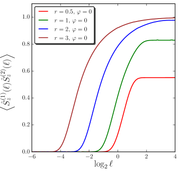
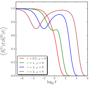
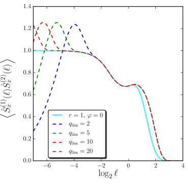
Unfortunately, the second quadrature cannot be performed analytically and has to be done numerically, and so has the sum appearing in Eq. (37). The results are presented in Fig. 8. In the left panel, $\langle\Psi_{2\,{\rm sq}}|\hat{S}^{(1)}_{z}(\ell)\hat{S}^{(2)}_{z}(\ell)|\Psi_{2\,{\rm sq}}\rangle$ is displayed versus $\log_{2}\ell$ for different values of the squeezing parameter and a vanishing squeezing angle. One can check that these curves are consistent with the results of LABEL:2004PhRvA..70b2102L (see Fig. 1 of that article). In the right panel, the same quantity is represented for $r=2$ and different values of the squeezing angle. These results are completely new to our knowledge. One can see that the overall structure of the correlation function is preserved, namely it vanishes at small $\ell$ and exhibits a plateau at large $\ell$, in agreement with the analytical limits of Secs. B.1 and B.2. However, when $\varphi\neq 0$, the correlation function can become negative.

The case $\varphi=\pi/4$ is even more intriguing since the correlation function vanishes regardless of the value of $\ell$. In fact, this can be understood analytically and allows us to check the consistency of our numerical calculations. Indeed, for $\varphi=\pi/4$, one has $\gamma_{1}=\gamma_{2}=2/\cosh(2r)$. From Eqs. (33) and (34), this implies that $A+A^{*}=-\gamma_{1}/2$ and $B+B^{*}=0$. As a consequence, Eq. (31) can be written as

$$Z_{n,m}\left(r,\varphi=\frac{\pi}{4}\right)=\int_{n\ell}^{(n+1)\ell}{\rm d}Q_{1}e^{-\gamma_{1}Q_{1}^{2}/2}\int_{m\ell}^{(m+1)\ell}{\rm d}Q_{2}e^{-\gamma_{1}Q_{2}^{2}/2}.$$ (38)

In other words, the two sub-systems are now “decoupled” and the two-point correlation function of the bipartite system is in fact the product of two one-point functions and must therefore vanish. Let us see how it works in practice. From Eq. (38), $Z_{n,m}$ can be calculated explicitly and reads

$$Z_{n,m}\left(r,\varphi=\frac{\pi}{4}\right)= \frac{\pi}{2\gamma_{1}}\left\{\operatorname{erf}\left[\ell\sqrt{\frac{\gamma_{1}}{2}}(n+1)\right]-\operatorname{erf}\left(\ell\sqrt{\frac{\gamma_{1}}{2}}n\right)\right\}\left\{\operatorname{erf}\left[\ell\sqrt{\frac{\gamma_{1}}{2}}(m+1)\right]-\operatorname{erf}\left(\ell\sqrt{\frac{\gamma_{1}}{2}}m\right)\right\}$$ (39)

$$= \frac{\pi}{2\gamma_{1}}z_{n}z_{m},$$ (40)

with $z_{n}\equiv\mathfrak{z}_{n+1}-\mathfrak{z}_{n}$ and $\mathfrak{z}_{n}\equiv\operatorname{erf}(n\ell\sqrt{\gamma_{1}/2})$. Then, from Eq. (30), it follows that

$$\langle\Psi_{2\,{\rm sq}}|\hat{S}^{(1)}_{z}(\ell)\hat{S}^{(2)}_{z}(\ell)|\Psi_{2\,{\rm sq}}\rangle =\frac{1}{4}\sum_{n=-\infty}^{\infty}(-1)^{n}z_{n}\sum_{m=-\infty}^{\infty}(-1)^{m}z_{m}.$$ (41)

But one has $\sum_{n=-\infty}^{\infty}(-1)^{n}z_{n}=\sum_{n=-\infty}^{\infty}(-1)^{n}(\mathfrak{z}_{n+1}-\mathfrak{z}_{n})=0$, where in the last expression we have used the fact that $\mathfrak{z}_{n}=-\mathfrak{z}_{-n}$. This explains why the correlation function vanishes in the case $\varphi=\pi/4$.

In fact, this result can also be understood as the consequence of the fact that the two-point correlator of $\hat{S}_{z}$ is odd with respect to $\varphi=\pi/4$ (hence vanishes at $\varphi=\pi/4$). Indeed, in the right panel of Fig. 8, one can notice that the correlation function for $\varphi=\pi/3$ is the opposite to that for $\varphi=\pi/6$. This can be understood as follows. Let us go back to Eq. (31) which, using Eqs. (33) and (34), can be rewritten as

$$Z_{n,m}(r,\varphi)=\int_{n\ell}^{(n+1)\ell}{\rm d}Q_{1}\int_{m\ell}^{(m+1)\ell}{\rm d}Q_{2}e^{-[\gamma_{1}(r,\varphi)+\gamma_{2}(r,\varphi)]\left(Q_{1}^{2}+Q_{2}^{2}\right)/4-[\gamma_{1}(r,\varphi)-\gamma_{2}(r,\varphi)]Q_{1}Q_{2}/2}\,.$$ (42)

From Eqs. (33) and (34), one can see that the functions $\gamma_{1}$ and $\gamma_{2}$ are related through $\gamma_{1,2}(r,\varphi)=\gamma_{2,1}(r,\pi/2-\varphi)$. This implies that

$$Z_{n,m}\left(r,\frac{\pi}{2}-\varphi\right) =\int_{n\ell}^{(n+1)\ell}{\rm d}Q_{1}\int_{m\ell}^{(m+1)\ell}{\rm d}Q_{2}e^{-[\gamma_{1}(r,\varphi)+\gamma_{2}(r,\varphi)]\left(Q_{1}^{2}+Q_{2}^{2}\right)/4+[\gamma_{1}(r,\varphi)-\gamma_{2}(r,\varphi)]Q_{1}Q_{2}/2}$$ (43)

$$=-\int_{n\ell}^{(n+1)\ell}{\rm d}Q_{1}\int_{-m\ell}^{-(m+1)\ell}{\rm d}Q_{2}e^{-[\gamma_{1}(r,\varphi)+\gamma_{2}(r,\varphi)]\left(Q_{1}^{2}+Q_{2}^{2}\right)/4-[\gamma_{1}(r,\varphi)-\gamma_{2}(r,\varphi)]Q_{1}Q_{2}/2},$$ (44)

where, in the last expression, we have changed the integration variable $Q_{2}$ to $-Q_{2}$. As a consequence, one can write that $Z_{n,m}(r,\pi/2-\varphi)=Z_{n,-m-1}(r,\varphi)$ and it follows that

$$\sum_{n=-\infty}^{\infty}\sum_{m=-\infty}^{\infty}(-1)^{n+m}Z_{n,m}\left(r,\frac{\pi}{2}-\varphi\right)=-\sum_{n=-\infty}^{\infty}\sum_{m^{\prime}=-\infty}^{\infty}(-1)^{n+m^{\prime}}Z_{n,m^{\prime}}\left(r,\varphi\right),$$ (45)

with $m^{\prime}=-m-1$. We have thus established that the correlation function evaluated with $r$ and $\varphi$ is minus the one calculated with $r$ and $\pi/2-\varphi$, and that these two configurations are therefore “dual” in a sense that will be further discussed in what follows, notably in Sec. E. This also means that one can study this correlation function in the interval $\varphi\in[0,\pi/4]$ only.

A.2 Correlation Function $\langle\Psi_{2\,{\rm sq}}|\hat{S}^{(1)}_{x}(\ell)\hat{S}^{(2)}_{x}(\ell)|\Psi_{2\,{\rm sq}}\rangle$

Figure 9: $\gamma_{3}$ (left panel) and $\gamma_{4}$ (right panel) defined in Eqs. (57) and (58), as a function of $r$, for $\varphi=0$, $\pi/6$, $\pi/4$, $\pi/3$, $\pi/2.3$ and $\pi/2$.

Let us now calculate the two-point correlation function of the operator $\hat{S}_{x}(\ell)$. Using its definition in terms of the spin step operators, see Eq. (10), $\hat{S}_{x}(\ell)=\hat{S}_{+}(\ell)+\hat{S}_{-}(\ell)$, one has

$$\langle\Psi_{2\,{\rm sq}}|\hat{S}^{(1)}_{x}(\ell)\hat{S}^{(2)}_{x}(\ell)|\Psi_{2\,{\rm sq}}\rangle= \langle\Psi_{2\,{\rm sq}}|\hat{S}^{(1)}_{+}(\ell)\hat{S}^{(2)}_{+}(\ell)|\Psi_{2\,{\rm sq}}\rangle+\langle\Psi_{2\,{\rm sq}}|\hat{S}^{(1)}_{-}(\ell)\hat{S}^{(2)}_{-}(\ell)|\Psi_{2\,{\rm sq}}\rangle$$

$$+\langle\Psi_{2\,{\rm sq}}|\hat{S}^{(1)}_{+}(\ell)\hat{S}^{(2)}_{-}(\ell)|\Psi_{2\,{\rm sq}}\rangle+\langle\Psi_{2\,{\rm sq}}|\hat{S}^{(1)}_{-}(\ell)\hat{S}^{(2)}_{+}(\ell)|\Psi_{2\,{\rm sq}}\rangle$$ (46)

$$= 2\Re\mathrm{e}\left[\langle\Psi_{2\,{\rm sq}}|\hat{S}^{(1)}_{+}(\ell)\hat{S}^{(2)}_{+}(\ell)|\Psi_{2\,{\rm sq}}\rangle+\langle\Psi_{2\,{\rm sq}}|\hat{S}^{(1)}_{+}(\ell)\hat{S}^{(2)}_{-}(\ell)|\Psi_{2\,{\rm sq}}\rangle\right]\,,$$ (47)

where we have used the relation $\hat{S}_{+}(\ell)=\hat{S}_{-}^{\dagger}(\ell)$ and the fact that the two-mode squeezed state is symmetric if one exchanges the sub-spaces $(1)$ and $(2)$, see Eq. (27). Therefore, one has to calculate two quantities. The first one is given by

$$\langle\Psi_{2\,{\rm sq}}|\hat{S}^{(1)}_{+}(\ell)\hat{S}^{(2)}_{+}(\ell)|\Psi_{2\,{\rm sq}}\rangle =\sum_{n=-\infty}^{\infty}\sum_{m=-\infty}^{\infty}\int_{2n\ell}^{(2n+1)\ell}{\rm d}Q_{1}\int_{2m\ell}^{(2m+1)\ell}{\rm d}Q_{2}\Psi_{\rm 2\,sq}^{*}\left(Q_{1},Q_{2}\right)\Psi_{\rm 2\,sq}\left(Q_{1}+\ell,Q_{2}+\ell\right)$$ (48)

$$=\frac{1}{\pi\cosh^{2}r}\frac{1}{\sqrt{\tanh^{4}r-2\tanh^{2}r\cos(4\varphi)+1}}\sum_{n=-\infty}^{\infty}\sum_{m=-\infty}^{\infty}J_{n,m}$$ (49)

with

$$J_{n,m}\equiv\int_{2n\ell}^{(2n+1)\ell}{\rm d}Q_{1}\int_{2m\ell}^{(2m+1)\ell}{\rm d}Q_{2}e^{(2A-B)\ell^{2}}e^{(A+A^{*})\left(Q_{1}^{2}+Q_{2}^{2}\right)-(B+B^{*})Q_{1}Q_{2}+(2A-B)\ell\left(Q_{1}+Q_{2}\right)}\,.$$ (50)

This integral has a structure similar to that of $Z_{n,m}$ except that, in the argument of the exponential, there is now a term proportional to $Q_{1}+Q_{2}$. The second quantity that needs to be calculated reads

$$\langle\Psi_{2\,{\rm sq}}|\hat{S}^{(1)}_{+}(\ell)\hat{S}^{(2)}_{-}(\ell)|\Psi_{2\,{\rm sq}}\rangle =\sum_{n=-\infty}^{\infty}\sum_{m=-\infty}^{\infty}\int_{(2n+1)\ell}^{(2n+2)\ell}{\rm d}Q_{1}\int_{2m\ell}^{(2m+1)\ell}{\rm d}Q_{2}\Psi_{\rm 2\,sq}^{*}\left(Q_{1},Q_{2}\right)\Psi_{\rm 2\,sq}\left(Q_{1}-\ell,Q_{2}+\ell\right)$$ (51)

$$=\frac{1}{\pi\cosh^{2}r}\frac{1}{\sqrt{\tanh^{4}r-2\tanh^{2}r\cos(4\varphi)+1}}\sum_{n=-\infty}^{\infty}\sum_{m=-\infty}^{\infty}K_{n,m}$$ (52)

with

$$K_{n,m}=\int_{(2n+1)\ell}^{(2n+2)\ell}{\rm d}Q_{1}\int_{2m\ell}^{(2m+1)\ell}{\rm d}Q_{2}e^{(2A+B)\ell^{2}}e^{(A+A^{*})\left(Q_{1}^{2}+Q_{2}^{2}\right)-(B+B^{*})Q_{1}Q_{2}-(2A+B)\ell\left(Q_{1}-Q_{2}\right)}\,.$$ (53)

We notice that the argument of the exponential also contains a new type of terms, this time proportional to $Q_{1}-Q_{2}$. In order to have the same integral limits in Eqs. (50) and (53), it is convenient to perform the change of integration variables $y_{1}=Q_{1}-\ell$ and $y_{2}=Q_{2}$ in Eq. (53), which gives rise to the following expression

$$K_{n,m}=\int_{2n\ell}^{(2n+1)\ell}\mathrm{d}y_{1}\int_{2m\ell}^{(2m+1)\ell}\mathrm{d}y_{2}e^{(A^{*}+A)\ell^{2}}e^{(A+A^{*})\left(y_{1}^{2}+y_{2}^{2}\right)-(B+B^{*})y_{1}y_{2}+(2A^{*}-B)\ell y_{1}+(2A-B^{*})\ell y_{2}}\,.$$ (54)

Plugging the above results in Eq. (47), one can write the correlation function as

$$\langle\Psi_{2\,{\rm sq}}|\hat{S}^{(1)}_{x}(\ell)\hat{S}^{(2)}_{x}(\ell)|\Psi_{2\,{\rm sq}}\rangle =\frac{1}{\pi\cosh^{2}r}\frac{1}{\sqrt{\tanh^{4}r-2\tanh^{2}r\cos(4\varphi)+1}}\sum_{n=-\infty}^{\infty}\sum_{m=-\infty}^{\infty}X_{n,m}\,,$$ (55)

where the quantity $X_{n,m}$ is defined by

$$X_{n,m}\equiv 2\int_{2n\ell}^{(2n+1)\ell}{\rm d}y_{1}\int_{2m\ell}^{(2m+1)\ell}{\rm d}y_{2}e^{(A+A^{*})\left(y_{1}^{2}+y_{2}^{2}\right)-(B+B^{*})y_{1}y_{2}}$$

$$\Re\mathrm{e}\left[e^{(2A-B)\ell^{2}+(2A-B)\ell\left(y_{1}+y_{2}\right)}+e^{(A^{*}+A)\ell^{2}+(2A^{*}-B)\ell y_{1}+(2A-B^{*})\ell y_{2}}\right].$$ (56)

At this stage, it is convenient to introduce the new parameters $\gamma_{3}$ and $\gamma_{4}$, defined by

$$2A-B= -\frac{1}{\cosh(2r)+\cos(2\varphi)\sinh(2r)}-i\frac{2\tanh r\sin(2\varphi)}{\tanh^{2}r+2\tanh r\cos(2\varphi)+1}\equiv-\frac{\gamma_{1}}{2}+i\gamma_{3}$$ (57)

$$2A^{*}-B= -\frac{1}{\cosh(2r)+\cos(2\varphi)\sinh(2r)}-i\frac{2\tanh r\sin(2\varphi)}{\tanh^{2}r-2\tanh r\cos(2\varphi)+1}\equiv-\frac{\gamma_{1}}{2}+i\gamma_{4}\,.$$ (58)

We see that the problem can be described in terms of four real functions, $\gamma_{1}$, $\gamma_{2}$, $\gamma_{3}$ and $\gamma_{4}$, which is consistent with the fact that the quantum state is given in terms of two complex functions $A$ and $B$. In fact, one can show that $A-A^{*}=i(\gamma_{3}-\gamma_{4})/2$ and $B-B^{*}=-i(\gamma_{3}+\gamma_{4})$. Recalling that $A+A^{*}=-(\gamma_{1}+\gamma_{2})/4$ and $B+B^{*}=(\gamma_{1}-\gamma_{2})/2$, one can then express $X_{n,m}$ in terms of the $\gamma_{i}$ functions only. The corresponding formula reads

$$X_{n,m}= 2\int_{2n\ell}^{(2n+1)\ell}{\rm d}y_{1}\int_{2m\ell}^{(2m+1)\ell}{\rm d}y_{2}e^{-(\gamma_{1}+\gamma_{2})\left(y_{1}^{2}+y_{2}^{2}\right)/4-(\gamma_{1}-\gamma_{2})y_{1}y_{2}/2}\biggl{\{}e^{-\gamma_{1}\left[\ell^{2}+\ell\left(y_{1}+y_{2}\right)\right]/2}\cos\left[\gamma_{3}\ell^{2}+\gamma_{3}\ell\left(y_{1}+y_{2}\right)\right]$$

$$+e^{-(\gamma_{1}+\gamma_{2})\ell^{2}/4-\gamma_{1}/2\ell\left(y_{1}+y_{2}\right)}\cos\left[\gamma_{4}\ell\left(y_{1}-y_{2}\right)\right]\biggr{\}}\,.$$ (59)

At this stage, it is also interesting to notice that $\gamma_{3}$ and $\gamma_{4}$ satisfy $\gamma_{3,4}(r,\varphi)=\gamma_{3,4}(r,\varphi+\pi)$ and $\gamma_{3,4}(r,\pi/2+\varphi)=-\gamma_{3,4}(r,\pi/2-\varphi)$, the last minus sign being the only difference with the otherwise similar symmetry properties given in Sec. A.1 for $\gamma_{1}$ and $\gamma_{2}$. But since Eq. (59) is unchanged when one flips the sign of $\gamma_{3}$ and $\gamma_{4}$, this means that, as in Sec. A.1, one can study the correlation function in the interval $\varphi\in[0,\pi/2]$ and use these symmetries to extend the result to other values of $\varphi$. The next step consists in performing the same change of integration variables as in Sec. A.1, namely $y_{1}=u+v$ and $y_{2}=u-v$, since this allows us to perform one of the two quadratures. This leads to

$$X_{n,m} =4e^{-\gamma_{1}\ell^{2}/2}\int_{(n+m)\ell}^{(n+m+1/2)\ell}{\rm d}ue^{-\gamma_{1}u^{2}-\gamma_{1}\ell u}\cos\left[\gamma_{3}\ell\left(\ell+2u\right)\right]\int_{2n\ell-u}^{u-2m\ell}{\rm d}ve^{-\gamma_{2}v^{2}}$$

$$+4e^{-(\gamma_{1}+\gamma_{2})\ell^{2}/4}\int_{(n+m)\ell}^{(n+m+1/2)\ell}{\rm d}ue^{-\gamma_{1}u^{2}-\gamma_{1}\ell u}\int_{2n\ell-u}^{u-2m\ell}{\rm d}ve^{-\gamma_{2}v^{2}}\cos\left(2\gamma_{4}\ell v\right)$$

$$+4e^{-\gamma_{1}\ell^{2}/2}\int_{(n+m+1/2)\ell}^{(n+m+1)\ell}{\rm d}ue^{-\gamma_{1}u^{2}-\gamma_{1}\ell u/2}\cos\left[\gamma_{3}\ell\left(\ell+2u\right)\right]\int_{u-(2m+1)\ell}^{(2n+1)\ell-u}{\rm d}ve^{-\gamma_{2}v^{2}}$$

$$+4e^{-(\gamma_{1}+\gamma_{2})\ell^{2}/4}\int_{(n+m+1/2)\ell}^{(n+m+1)\ell}{\rm d}ue^{-\gamma_{1}u^{2}-\gamma_{1}\ell u}\int_{u-(2m+1)\ell}^{(2n+1)\ell-u}{\rm d}ve^{-\gamma_{2}v^{2}}\cos\left(2\gamma_{4}\ell v\right)$$ (60)

$$\equiv X_{n,m}^{(1)}+X_{n,m}^{(2)}+X_{n,m}^{(3)}+X_{n,m}^{(4)}\,.$$ (61)

Again the structure of the integrals $X_{n,m}^{(i)}$ is very similar to that of $Z_{n,m}$. The only differences originate from the fact that the arguments of the exponentials now contain a term linear in $u$, and a cosine function is present in the first and third integrals. As before, the integrals over $v$ can be performed by means of error functions and one obtains

$$X_{n,m}^{(1)} =\ell\sqrt{\frac{\pi}{\gamma_{2}}}e^{-\gamma_{1}\ell^{2}/2}\int_{0}^{1}{\rm d}ze^{-\gamma_{1}\ell^{2}(z+2n+2m)^{2}/4-\gamma_{1}\ell^{2}(z+2n+2m)/2}\cos\left[\gamma_{3}\ell^{2}(z+2n+2m+1)\right]$$

$$\times\left\{{\rm erf}\left[\frac{\ell}{2}\sqrt{\gamma_{2}}(z-2n+2m)\right]+{\rm erf}\left[\frac{\ell}{2}\sqrt{\gamma_{2}}(z+2n-2m)\right]\right\}\,,$$ (62)

$$X_{n,m}^{(2)} =\ell\sqrt{\frac{\pi}{\gamma_{2}}}e^{-\left[(\gamma_{1}+\gamma_{2})/4+\gamma_{4}^{2}/\gamma_{2}\right]\ell^{2}}\int_{0}^{1}{\rm d}ze^{-\gamma_{1}\ell^{2}(z+2n+2m)^{2}/4-\gamma_{1}\ell^{2}(z+2n+2m)/2}$$

$$\times\Re\mathrm{e}\biggl{\{}{\rm erf}\left[\frac{\ell}{2}\sqrt{\gamma_{2}}(z-2n+2m)+i\frac{\gamma_{4}}{\sqrt{\gamma_{2}}}\ell\right]+{\rm erf}\left[\frac{\ell}{2}\sqrt{\gamma_{2}}(z+2n-2m)+i\frac{\gamma_{4}}{\sqrt{\gamma_{2}}}\ell\right]\biggr{\}}\,,$$ (63)

$$X_{n,m}^{(3)} =\ell\sqrt{\frac{\pi}{\gamma_{2}}}e^{-\gamma_{1}\ell^{2}/2}\int_{0}^{1}{\rm d}ze^{-\gamma_{1}\ell^{2}(z-2n-2m-2)^{2}/4+\gamma_{1}\ell^{2}(z-2n-2m-2)/2}\cos\left[\gamma_{3}\ell^{2}(z-2n-2m-3)\right]$$

$$\times\left\{{\rm erf}\left[\frac{\ell}{2}\sqrt{\gamma_{2}}(z-2n+2m)\right]+{\rm erf}\left[\frac{\ell}{2}\sqrt{\gamma_{2}}(z+2n-2m)\right]\right\}\,,$$ (64)

$$X_{n,m}^{(4)} =\ell\sqrt{\frac{\pi}{\gamma_{2}}}e^{-\left[(\gamma_{1}+\gamma_{2})/4+\gamma_{4}^{2}/\gamma_{2}\right]\ell^{2}}\int_{0}^{1}{\rm d}ze^{-\gamma_{1}\ell^{2}(z-2n-2m-2)^{2}/4+\gamma_{1}\ell^{2}(z-2n-2m-2)/2}$$

$$\times\Re\mathrm{e}\biggl{\{}{\rm erf}\left[\frac{\ell}{2}\sqrt{\gamma_{2}}(z-2n+2m)+i\frac{\gamma_{4}}{\sqrt{\gamma_{2}}}\ell\right]+{\rm erf}\left[\frac{\ell}{2}\sqrt{\gamma_{2}}(z+2n-2m)+i\frac{\gamma_{4}}{\sqrt{\gamma_{2}}}\ell\right]\biggr{\}}\,.$$ (65)

Finally, the expression of the spin correlation function can be written as

$$\langle\Psi_{2\,{\rm sq}}|\hat{S}^{(1)}_{x}(\ell)\hat{S}^{(2)}_{x}(\ell)|\Psi_{2\,{\rm sq}}\rangle =\frac{\sqrt{\gamma_{1}\gamma_{2}}}{2\pi}\sum_{n=-\infty}^{\infty}\sum_{m=-\infty}^{\infty}\left[X^{(1)}_{n,m}+X^{(2)}_{n,m}+X^{(3)}_{n,m}+X^{(4)}_{n,m}\right]\,.$$ (66)

Figure 10: Two-point correlator $\langle\Psi_{2\,{\rm sq}}|\hat{S}^{(1)}_{x}(\ell)\hat{S}^{(2)}_{x}(\ell)|\Psi_{2\,{\rm sq}}\rangle$ as a function of $\ell$, for $\varphi=0$ and a few values of $r$ (left panel), and $r=2$ and a few values of $\varphi$ (right panel).

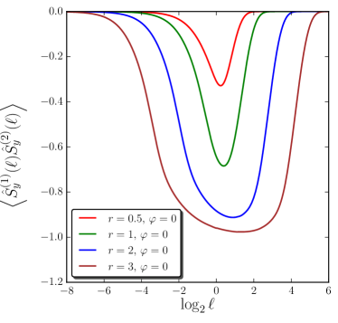
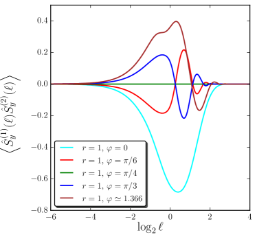
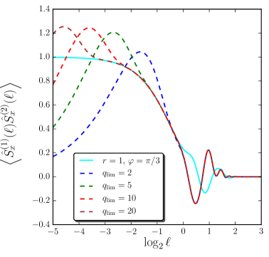
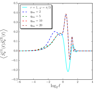
As it was already the case for the integrals $Z_{n,m}$, the remaining integrals need to be performed numerically, and so do the sums over $n$ and $m$. The result is displayed in Fig. 10. In the left panel, the correlation function is given for different values of $r$ and a vanishing squeezing angle. Our curves are consistent with those of LABEL:2004PhRvA..70b2102L even if the systematic shift already observed for the correlation function $\langle\Psi_{2\,{\rm sq}}|\hat{S}^{(1)}_{z}(\ell)\hat{S}^{(2)}_{z}(\ell)|\Psi_{2\,{\rm sq}}\rangle$ is still present. In the right panel, results for $r=1$ and different squeezing angles are displayed. We notice that the small and large $\ell$ limits (namely one and zero, respectively) are not affected by the fact that $\varphi\neq 0$, see the analytical results of Secs. B.1 and B.2. Only the structure between these two regimes is changed. In particular, we see some oscillatory patterns originating from the fact that the integrals $X_{n,m}^{(i)}$ contain cosine functions and complex error functions.

We also notice that $\langle\Psi_{2\,{\rm sq}}|\hat{S}^{(1)}_{x}(\ell)\hat{S}^{(2)}_{x}(\ell)|\Psi_{2\,{\rm sq}}\rangle$ for $\varphi=\pi/6$ (solid blue line) and $\varphi=\pi/3$ (solid red line) are exactly equal. This is a consequence of the fact that this correlation function is even with respect to $\varphi=\pi/4$. Indeed, from Eqs. (57) and (58), one can check that the functions $\gamma_{3}$ and $\gamma_{4}$ satisfy the same additional symmetry as $\gamma_{1}$ and $\gamma_{2}$, namely $\gamma_{3,4}(r,\varphi)=\gamma_{4,3}(r,\pi/2-\varphi)$. Using this property in Eq. (59), one obtains

$$X_{n,m}\left(r,\frac{\pi}{2}-\varphi\right)= 2\int_{2n\ell}^{(2n+1)\ell}{\rm d}y_{1}\int_{2m\ell}^{(2m+1)\ell}{\rm d}y_{2}e^{-(\gamma_{1}+\gamma_{2})\left(y_{1}^{2}+y_{2}^{2}\right)/4+(\gamma_{1}-\gamma_{2})y_{1}y_{2}/2}\biggl{\{}e^{-\gamma_{2}\left[\ell^{2}+\ell\left(y_{1}+y_{2}\right)\right]/2}$$

$$\times\cos\left[\gamma_{4}\ell^{2}+\gamma_{4}\ell\left(y_{1}+y_{2}\right)\right]+e^{-(\gamma_{1}+\gamma_{2})\ell^{2}/4-\gamma_{2}/2\ell\left(y_{1}+y_{2}\right)}\cos\left[\gamma_{3}\ell\left(y_{1}-y_{2}\right)\right]\biggr{\}}\,,$$ (67)

with all $\gamma_{i}$ functions evaluated at $r$ and $\varphi$. Let us then perform the change of integration variable $y_{2}\rightarrow-y_{2}-\ell$. After straightforward manipulations, it is easy to show that $X_{n,m}\left(r,\pi/2-\varphi\right)=X_{n,-m-1}\left(r,\varphi\right)$. As a consequence, one has $\sum_{n=-\infty}^{\infty}\sum_{m=-\infty}^{\infty}X_{n,m}(r,\pi/2-\varphi)=\sum_{n=-\infty}^{\infty}\sum_{m=-\infty}^{\infty}X_{n,m}(r,\varphi)$. This confirms that $\langle\Psi_{2\,{\rm sq}}|\hat{S}^{(1)}_{x}(\ell)\hat{S}^{(2)}_{x}(\ell)|\Psi_{2\,{\rm sq}}\rangle$ is even with respect to $\varphi=\pi/4$, hence one can restrict the present analysis to $\varphi\in[0,\pi/4]$. This also checks the validity of our numerical computation in the cases $\varphi=\pi/6$ and $\varphi=\pi/3$.

A.3 Correlation Function $\langle\Psi_{2\,{\rm sq}}|\hat{S}^{(1)}_{y}(\ell)\hat{S}^{(2)}_{y}(\ell)|\Psi_{2\,{\rm sq}}\rangle$.

Figure 11: Two-point correlator $\langle\Psi_{2\,{\rm sq}}|\hat{S}^{(1)}_{y}(\ell)\hat{S}^{(2)}_{y}(\ell)|\Psi_{2\,{\rm sq}}\rangle$ as a function of $\ell$, for $\varphi=0$ and a few values of $r$ (left panel), and $r=2$ and a few values of $\varphi$ (right panel).

Let us then calculate the two-point correlation function of the operator $\hat{S}_{y}(\ell)$. Since, see Eq. (11), one has $\hat{S}_{y}(\ell)=-i[\hat{S}_{+}(\ell)-\hat{S}_{-}(\ell)]$, one can write

$$\langle\Psi_{2\,{\rm sq}}|\hat{S}^{(1)}_{y}(\ell)\hat{S}^{(2)}_{y}(\ell)|\Psi_{2\,{\rm sq}}\rangle= -\langle\Psi_{2\,{\rm sq}}|\hat{S}^{(1)}_{+}(\ell)\hat{S}^{(2)}_{+}(\ell)|\Psi_{2\,{\rm sq}}\rangle-\langle\Psi_{2\,{\rm sq}}|\hat{S}^{(1)}_{-}(\ell)\hat{S}^{(2)}_{-}(\ell)|\Psi_{2\,{\rm sq}}\rangle$$

$$+\langle\Psi_{2\,{\rm sq}}|\hat{S}^{(1)}_{+}(\ell)\hat{S}^{(2)}_{-}(\ell)|\Psi_{2\,{\rm sq}}\rangle+\langle\Psi_{2\,{\rm sq}}|\hat{S}^{(1)}_{-}(\ell)\hat{S}^{(2)}_{+}(\ell)|\Psi_{2\,{\rm sq}}\rangle$$ (68)

$$= 2\Re\mathrm{e}\left[\langle\Psi_{2\,{\rm sq}}|\hat{S}^{(1)}_{+}(\ell)\hat{S}^{(2)}_{-}(\ell)|\Psi_{2\,{\rm sq}}\rangle-\langle\Psi_{2\,{\rm sq}}|\hat{S}^{(1)}_{+}(\ell)\hat{S}^{(2)}_{+}(\ell)|\Psi_{2\,{\rm sq}}\rangle\right]\,,$$ (69)

where, as in Sec. A.2, we have used the relation $\hat{S}_{+}(\ell)=\hat{S}_{-}^{\dagger}(\ell)$ and the fact that the two-mode squeezed state is symmetric in $(1)\leftrightarrow(2)$. Comparing this formula with Eq. (47), one can see that the calculation one has to perform is exactly the same, up to two sign differences and one obtains

$$\langle\Psi_{2\,{\rm sq}}|\hat{S}^{(1)}_{y}(\ell)\hat{S}^{(2)}_{y}(\ell)|\Psi_{2\,{\rm sq}}\rangle =\frac{\sqrt{\gamma_{1}\gamma_{2}}}{2\pi}\sum_{n,m}\left[-X^{(1)}_{n,m}-X^{(3)}_{n,m}+X^{(2)}_{n,m}+X^{(4)}_{n,m}\right]\,.$$ (70)

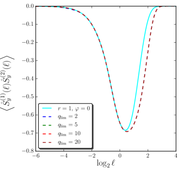
This correlation function is displayed in Fig. 11. The left panel represents $\langle\Psi_{2\,{\rm sq}}|\hat{S}^{(1)}_{y}(\ell)\hat{S}^{(2)}_{y}(\ell)|\Psi_{2\,{\rm sq}}\rangle$ for different values of $r$ and a vanishing squeezing angle while the right panel is for $r=1$ and different squeezing angles. The correlation function vanishes at small and large $\ell$, in agreement with the analytical results of Secs. B.1 and B.2. Otherwise, the same remarks as the ones made for $\langle\Psi_{2\,{\rm sq}}|\hat{S}^{(1)}_{x}(\ell)\hat{S}^{(2)}_{x}(\ell)|\Psi_{2\,{\rm sq}}\rangle$ are still valid in the present case and, therefore, need not be repeated here. In particular, the same correspondence between $\varphi$ and $\pi/2-\varphi$ takes place, so that these two configurations are “dual” and connected through the formulas

$$\langle\Psi_{2\,{\rm sq}}|\hat{S}^{(1)}_{z}(\ell)\hat{S}^{(2)}_{z}(\ell)|\Psi_{2\,{\rm sq}}\rangle\left(r,\pi/2-\varphi\right) =-\langle\Psi_{2\,{\rm sq}}|\hat{S}^{(1)}_{z}(\ell)\hat{S}^{(2)}_{z}(\ell)|\Psi_{2\,{\rm sq}}\rangle\left(r,\varphi\right)\,,$$ (71)

$$\langle\Psi_{2\,{\rm sq}}|\hat{S}^{(1)}_{x}(\ell)\hat{S}^{(2)}_{x}(\ell)|\Psi_{2\,{\rm sq}}\rangle\left(r,\pi/2-\varphi\right) =\langle\Psi_{2\,{\rm sq}}|\hat{S}^{(1)}_{x}(\ell)\hat{S}^{(2)}_{x}(\ell)|\Psi_{2\,{\rm sq}}\rangle\left(r,\varphi\right)\,,$$ (72)

$$\langle\Psi_{2\,{\rm sq}}|\hat{S}^{(1)}_{y}(\ell)\hat{S}^{(2)}_{y}(\ell)|\Psi_{2\,{\rm sq}}\rangle\left(r,\pi/2-\varphi\right) =-\langle\Psi_{2\,{\rm sq}}|\hat{S}^{(1)}_{y}(\ell)\hat{S}^{(2)}_{y}(\ell)|\Psi_{2\,{\rm sq}}\rangle\left(r,\varphi\right)\,.$$ (73)

A.4 Correlation Function $\langle\Psi_{2\,{\rm sq}}|\hat{S}^{(1)}_{x}(\ell)\hat{S}^{(2)}_{z}(\ell)|\Psi_{2\,{\rm sq}}\rangle$.

Let us finally calculate the cross correlation function of the operators $\hat{S}_{x}(\ell)$ and $\hat{S}_{z}(\ell)$. Since $\hat{S}_{x}(\ell)=\hat{S}_{+}(\ell)+\hat{S}_{-}(\ell)$, see Eq. (10), one has

$$\langle\Psi_{2\,{\rm sq}}|\hat{S}^{(1)}_{x}(\ell)\hat{S}^{(2)}_{z}(\ell)|\Psi_{2\,{\rm sq}}\rangle= \langle\Psi_{2\,{\rm sq}}|\hat{S}^{(1)}_{+}(\ell)\hat{S}^{(2)}_{z}(\ell)|\Psi_{2\,{\rm sq}}\rangle+\langle\Psi_{2\,{\rm sq}}|\hat{S}^{(1)}_{-}(\ell)\hat{S}^{(2)}_{z}(\ell)|\Psi_{2\,{\rm sq}}\rangle$$ (74)

$$= \langle\Psi_{2\,{\rm sq}}|\hat{S}^{(1)}_{+}(\ell)\hat{S}^{(2)}_{z}(\ell)|\Psi_{2\,{\rm sq}}\rangle+\langle\Psi_{2\,{\rm sq}}|\hat{S}^{(1)}_{z}(\ell)\hat{S}^{(2)}_{-}(\ell)|\Psi_{2\,{\rm sq}}\rangle$$ (75)

$$= 2\Re\mathrm{e}\left[\langle\Psi_{2\,{\rm sq}}|\hat{S}^{(1)}_{+}(\ell)\hat{S}^{(2)}_{z}(\ell)|\Psi_{2\,{\rm sq}}\rangle\right]\,,$$ (76)

where, in Eq. (75), one has used the fact that the two-mode squeezed state is symmetric if one exchanges the sub-spaces $(1)$ and $(2)$, see Eq. (27), and where in Eq. (76), one has used that $S_{+}(\ell)=S_{-}^{\dagger}(\ell)$. One therefore has to calculate the quantity

$$\langle\Psi_{2\,{\rm sq}}|\hat{S}^{(1)}_{+}(\ell)\hat{S}^{(2)}_{z}(\ell)|\Psi_{2\,{\rm sq}}\rangle =\sum_{n=-\infty}^{\infty}\sum_{m=-\infty}^{\infty}(-1)^{n}\int_{n\ell}^{(n+1)\ell}{\rm d}Q_{1}\int_{2m\ell}^{(2m+1)\ell}{\rm d}Q_{2}\Psi_{\rm 2\,sq}^{*}\left(Q_{1},Q_{2}\right)\Psi_{\rm 2\,sq}\left(Q_{1}+\ell,Q_{2}\right)$$ (77)

$$=\frac{1}{\pi\cosh^{2}r}\frac{1}{\sqrt{\tanh^{4}r-2\tanh^{2}r\cos(4\varphi)+1}}\sum_{n=-\infty}^{\infty}\sum_{m=-\infty}^{\infty}(-1)^{n}L_{n,m}$$ (78)

with

$$L_{n,m}=\int_{n\ell}^{(n+1)\ell}{\rm d}Q_{1}\int_{2m\ell}^{(2m+1)\ell}{\rm d}Q_{2}e^{A\ell^{2}}e^{(A+A_{*})(Q_{1}^{2}+Q_{2}^{2})-(B+B_{*})Q_{1}Q_{2}+(2AQ_{1}-BQ_{2})\ell}\,.$$ (79)

Let us now perform the same change of integration variable as in Sec. A.1, namely $Q_{1}=u+v$ and $Q_{2}=u-v$. As a consequence, one obtains

$$L_{n,m} =2e^{A\ell^{2}}\int_{(n+2m)\ell/2}^{(n+2m+1)\ell/2}\mathrm{d}ue^{-\gamma_{1}u^{2}-\left(\frac{\gamma_{1}}{2}-i\gamma_{3}\right)\ell u}\int_{n\ell-u}^{u-2m\ell}\mathrm{d}ve^{-\gamma_{2}v^{2}-\left(\frac{\gamma_{2}}{2}+i\gamma_{4}\right)\ell v}$$

$$+2e^{A\ell^{2}}\int_{(n+2m+1)\ell/2}^{(n+2m+2)\ell/2}\mathrm{d}ue^{-\gamma_{1}u^{2}-\left(\frac{\gamma_{1}}{2}-i\gamma_{3}\right)\ell u}\int_{u-(2m+1)\ell}^{(n+1)\ell-u}\mathrm{d}ve^{-\gamma_{2}v^{2}-\left(\frac{\gamma_{2}}{2}+i\gamma_{4}\right)\ell v}\equiv L_{n,m}^{(1)}+L_{n,m}^{(2)}\,.$$ (80)

Similarly as before, the change of integration variable $z=2u/\ell-n-2m$ in $L_{n,m}^{(1)}$ and $z=-2u/\ell+n+2m+2$ in $L_{n,m}^{(2)}$ leads to

$$L_{n,m}^{(1)} =\ell e^{A\ell^{2}}\int_{0}^{1}\mathrm{d}ze^{-\gamma_{1}u^{2}-\left(\frac{\gamma_{1}}{2}-i\gamma_{3}\right)\ell u}\int_{(n-2m-z)\ell/2}^{(n-2m+z)\ell/2}\mathrm{d}ve^{-\gamma_{2}v^{2}-\left(\frac{\gamma_{2}}{2}+i\gamma_{4}\right)\ell v}$$ (81)

$$L_{n,m}^{(2)} =\ell e^{A\ell^{2}}\int_{0}^{1}\mathrm{d}ze^{-\gamma_{1}u^{2}-\left(\frac{\gamma_{1}}{2}-i\gamma_{3}\right)\ell u}\int^{(n-2m-z)\ell/2}_{(n-2m+z)\ell/2}\mathrm{d}ve^{-\gamma_{2}v^{2}-\left(\frac{\gamma_{2}}{2}+i\gamma_{4}\right)\ell v}\,.$$ (82)

These two expressions are the same, except that the lower and upper bounds of the integral over $v$ are inverted, hence $L_{n,m}^{(1)}=-L_{n,m}^{(2)}$ and $L_{n,m}=0$. We have thus shown that $\langle\Psi_{2\,{\rm sq}}|\hat{S}^{(1)}_{+}(\ell)\hat{S}^{(2)}_{z}(\ell)|\Psi_{2\,{\rm sq}}\rangle=0$, and consequently

$$\langle\Psi_{2\,{\rm sq}}|\hat{S}^{(1)}_{x}(\ell)\hat{S}^{(2)}_{z}(\ell)|\Psi_{2\,{\rm sq}}\rangle=0\,,$$ (83)

that is to say measurements along orthogonal directions are uncorrelated for the two-mode squeezed state.

Having established the exact (numerical) form of the spin correlation functions, we now turn to the question of finding analytical approximations.

Appendix B Large and Small $\ell$ Limits

In Figs. 8, 10 and 11, one can see that the two-point correlation functions of the spin operators reach constant values at small and large $\ell$. In this section, we derive the analytical expressions of the corresponding asymptotic values.

B.1 The large $\ell$ limit

Let us first consider the asymptotic behavior of the correlation functions at large $\ell$. We start by treating the correlation function of the $z$-component of the spin. One can notice that the integration domains appearing in $Z_{n,m}^{(1)}$ defined in Eq. (32) are of two kinds. Either they contain the point $(u=0,v=0)$, close to which the integrand is maximal, either they do not. In the second case, when $\ell\gg 1$, the integrand is exponentially suppressed and the corresponding value for $Z_{n,m}^{(1)}$ negligibly contributes to the overall sum (37). Therefore, in the $\ell\gg 1$ limit, it is enough to keep the contributions from the first kind of integrals only. It is easy to see that three terms are of this first kind, namely $Z_{0,0}^{(1)}$, $Z_{-1,0}^{(1)}$ and $Z_{0,-1}^{(1)}$. In the limit $\ell\rightarrow\infty$, they are given by

$$Z_{0,0}^{(1)} \simeq 2\int_{0}^{\infty}\mathrm{d}ue^{-\gamma_{1}u^{2}}\int_{-u}^{u}\mathrm{d}ve^{-\gamma_{2}v^{2}}\,,\quad Z_{-1,0}^{(1)}\simeq 2\int_{-\infty}^{0}\mathrm{d}ue^{-\gamma_{1}u^{2}}\int_{-\infty}^{u}\mathrm{d}ve^{-\gamma_{2}v^{2}}\,,$$ (84)

$$Z_{0,-1}^{(1)} \simeq 2\int_{-\infty}^{0}\mathrm{d}ue^{-\gamma_{1}u^{2}}\int_{-u}^{\infty}\mathrm{d}ve^{-\gamma_{2}v^{2}}\,.$$ (85)

As a consequence, the sum appearing in Eq. (37) can be written as

$$\sum_{n,m}(-1)^{n+m}Z_{n,m}^{(1)} \simeq Z_{0,0}^{(1)}-Z_{-1,0}^{(1)}-Z_{0,-1}^{(1)}=2\int_{0}^{\infty}\mathrm{d}ue^{-\gamma_{1}u^{2}}\left(\int_{-u}^{u}\mathrm{d}ve^{-\gamma_{2}v^{2}}-2\int_{u}^{\infty}\mathrm{d}ve^{-\gamma_{2}v^{2}}\right)$$ (86)

$$=2\sqrt{\frac{\pi}{\gamma_{2}}}\int_{0}^{\infty}\mathrm{d}ue^{-\gamma_{1}u^{2}}\left[2\operatorname{erf}\left(u\sqrt{\gamma_{2}}\right)-1\right]=\frac{2}{\sqrt{\gamma_{1}\gamma_{2}}}\left[2\arctan\left(\sqrt{\frac{\gamma_{2}}{\gamma_{1}}}\right)-\frac{\pi}{2}\right]\,.$$ (87)

This formula can be simplified and it is convenient to rewrite it as

$$\sum_{n,m}(-1)^{n+m}Z_{n,m}^{(1)}\simeq\frac{2}{\sqrt{\gamma_{1}\gamma_{2}}}\arctan\left(\frac{\gamma_{2}-\gamma_{1}}{2\sqrt{\gamma_{1}\gamma_{2}}}\right)\,.$$ (89)

Making use of Eqs. (37), (33) and (34), the last equation can expressed explicitly in terms of the squeezing parameter $r$ and squeezing parameter angle $\varphi$. One eventually obtains

$$\langle\Psi_{2\,{\rm sq}}|\hat{S}^{(1)}_{z}(\ell)\hat{S}^{(2)}_{z}(\ell)|\Psi_{2\,{\rm sq}}\rangle\simeq\frac{2}{\pi}\arctan\left[\frac{\cos(2\varphi)\sinh(2r)}{\sqrt{\cosh^{2}(2r)-\cos^{2}(2\varphi)\sinh^{2}(2r)}}\right]\,.$$ (90)

In the case where $\varphi=0$, one obtains $\langle\Psi_{2\,{\rm sq}}|\hat{S}^{(1)}_{z}(\ell)\hat{S}^{(2)}_{z}(\ell)|\Psi_{2\,{\rm sq}}\rangle\simeq 2\arctan[\sinh(2r)]/\pi$, in agreement with Eq. (17) of LABEL:2004PhRvA..70b2102L, but the expression derived here is more general. The asymptotic plateau given by Eq. (90) is compared to the numerical curve obtained from Eq. (37) in Fig. 12 (black line), and one can check that the agreement is indeed excellent.

The same strategy can be employed to approximate the correlation functions of $\hat{S}_{x}(\ell)$ and $\hat{S}_{y}(\ell)$ in the large $\ell$ limit. From Eq. (60), it is clear that no integration domain in $X_{n,m}$ is of the first kind [i.e. contains the point $(u,v)=(0,0)$] and therefore, $\langle\Psi_{2\,{\rm sq}}|\hat{S}^{(1)}_{x}(\ell)\hat{S}^{(2)}_{x}(\ell)|\Psi_{2\,{\rm sq}}\rangle\simeq\langle\Psi_{2\,{\rm sq}}|\hat{S}^{(1)}_{y}(\ell)\hat{S}^{(2)}_{y}(\ell)|\Psi_{2\,{\rm sq}}\rangle\simeq 0$ in this limit.

B.2 The small $\ell$ limit

Let us now consider the asymptotic behavior of the correlation functions in the opposite limit, $\ell\ll 1$. As before, we first consider the correlation function for the $z$-component of the spin. Since $\ell$ is small, one can simplify the integrand in Eq. (35) by expanding the error functions around $\ell\sqrt{\gamma_{2}}(n-m)/2$:

$${\operatorname{erf}}\left[\frac{\ell}{2}\sqrt{\gamma_{2}}\left(z+n-m\right)\right]+{\operatorname{erf}}\left[\frac{\ell}{2}\sqrt{\gamma_{2}}\left(z-n+m\right)\right] ={\operatorname{erf}}\left[\frac{\ell}{2}\sqrt{\gamma_{2}}\left(n-m+z\right)\right]-{\operatorname{erf}}\left[\frac{\ell}{2}\sqrt{\gamma_{2}}\left(n-m-z\right)\right]$$ (91)

$$\simeq 2\ell\sqrt{\frac{\gamma_{2}}{\pi}}e^{-\ell^{2}\gamma_{2}(n-m)^{2}/4}z\,.$$ (92)

One then has

$$Z_{n,m}^{(1)} \simeq\ell^{2}e^{-\ell^{2}\gamma_{2}(n-m)^{2}/4}\int_{0}^{1}\mathrm{d}ze^{-\gamma_{1}\ell^{2}(z+n+m)^{2}/4}z\,.$$ (93)

This integral can be expressed in terms of the error function. Alternatively, one can notice that when $\ell\ll 1$, the argument of the exponential in the integrand vanishes, except if $|n+m|\gg 1$. In the later case, $z+n+m\simeq n+m$ and one can therefore replace $z$ by $0$ in the argument of the exponential in this limit. As a consequence, one obtains

$$Z_{n,m}^{(1)} \simeq\frac{\ell^{2}}{2}e^{-\frac{\ell^{2}}{4}\left[\gamma_{2}(n-m)^{2}+\gamma_{1}(n+m)^{2}\right]}\,.$$ (94)

In this expression, only the combinations $n-m$ and $n+m$ are involved. Defining $p\equiv n+m$ and $q\equiv n-m$, it follows that the sum appearing in Eq. (37) can be written as

$$\sum_{n,m=-\infty}^{\infty}(-1)^{n+m}Z_{n,m}^{(1)}=\sum_{q=-\infty}^{\infty}\mathcal{Z}_{q}^{(1)}\sum_{p\in\mathcal{P}(q)}\mathcal{Z}_{p}^{(1)}\,,$$ (95)

where the quantities $\mathcal{Z}_{q}^{(1)}$ and $\mathcal{Z}_{p}^{(1)}$ are defined by

$$\mathcal{Z}_{q}^{(1)}=\frac{\ell^{2}}{2}e^{-\gamma_{2}q^{2}\frac{\ell^{2}}{4}}\,,\quad\quad\mathcal{Z}_{p}^{(1)}=(-1)^{p}e^{-\gamma_{1}p^{2}\frac{\ell^{2}}{4}}\,.$$ (96)

In Eq. (95), the symbol $\mathcal{P}(q)$ stands for all integer numbers having the same parity as $q$. Therefore, if $q$ is even, the sum over $p$ can be expressed as

$$\sum_{p\in\mathcal{P}(q)}\mathcal{Z}_{p}^{(1)}=\sum_{p^{\prime}=-\infty}^{\infty}\mathcal{Z}_{2p^{\prime}}^{(1)}=\sum_{p^{\prime}=-\infty}^{\infty}e^{-\gamma_{1}{p^{\prime}}^{2}\ell^{2}}=\vartheta_{3}\left(0,e^{-\gamma_{1}\ell^{2}}\right)$$ (97)

where $\vartheta_{3}$ is the third Jacobi function Gradshteyn and Ryzhik (1965). On the other hand, if $q$ is odd, this sum can be written as

$$\sum_{p\in\mathcal{P}(q)}\mathcal{Z}_{p}^{(1)}=\sum_{p^{\prime}=-\infty}^{\infty}\mathcal{Z}_{2p^{\prime}+1}^{(1)}=-\sum_{p^{\prime}=-\infty}^{\infty}e^{-\gamma_{1}\left(p^{\prime}+\frac{1}{2}\right)^{2}\ell^{2}}=-\vartheta_{2}\left(0,e^{-\gamma_{1}\ell^{2}}\right)$$ (98)

where $\vartheta_{2}$ is the second Jacobi function Gradshteyn and Ryzhik (1965). When $\ell\ll 1$, the behavior of the two Jacobi functions is similar and one obtains

$$\sum_{n,m=-\infty}^{\infty}(-1)^{n+m}Z_{n,m}^{(1)} =\sqrt{\frac{\pi}{\gamma_{1}}}\frac{\ell}{2}\left[\sum_{q=-\infty}^{\infty}e^{-\gamma_{2}q^{2}\ell^{2}}-\sum_{q=-\infty}^{\infty}e^{-\gamma_{2}\left(q+\frac{1}{2}\right)^{2}\ell^{2}}\right]$$ (99)

$$=\sqrt{\frac{\pi}{\gamma_{1}}}\frac{\ell}{2}\left[\vartheta_{3}\left(0,e^{-\gamma_{2}\ell^{2}}\right)-\vartheta_{2}\left(0,e^{-\gamma_{2}\ell^{2}}\right)\right]\simeq\frac{2\pi}{\sqrt{\gamma_{1}\gamma_{2}}}e^{-\frac{\pi^{2}}{\gamma_{2}\ell^{2}}},$$ (100)

where in the last expression one has used the limit $\ell\ll 1$ again. Since $\gamma_{2}>0$, this means that $\langle\Psi_{2\,{\rm sq}}|\hat{S}^{(1)}_{z}(\ell)\hat{S}^{(2)}_{z}(\ell)|\Psi_{2\,{\rm sq}}\rangle$ vanishes when $\ell\rightarrow 0$ in accordance with what is observed in Figs. 8.

The same calculation can be performed for the correlation functions of the $x$- and $y$- components of the spin. Let us first express $X_{n,m}^{(1)}$, $X_{n,m}^{(2)}$, $X_{n,m}^{(3)}$ and $X_{n,m}^{(4)}$ in the $\ell\ll 1$ limit. In Eqs. (A.2) and (A.2), the error functions can be expanded around $\ell\sqrt{\gamma_{2}}(n-m)$ and one obtains

$$\operatorname{erf}\left[\frac{\ell}{2}\sqrt{\gamma_{2}}(z-2n+2m)\right]+\operatorname{erf}\left[\frac{\ell}{2}\sqrt{\gamma_{2}}(z+2n-2m)\right]\simeq 2\ell\sqrt{\frac{\gamma_{2}}{\pi}}e^{-\ell^{2}\gamma_{2}(n-m)^{2}}z\,.$$ (101)

One then has

$$X_{n,m}^{(1)} \simeq 2\ell^{2}e^{-\gamma_{1}\ell^{2}/2-\gamma_{2}(n-m)^{2}\ell^{2}}\int_{0}^{1}{\rm d}ze^{-\gamma_{1}\ell^{2}(z+2n+2m)^{2}/4-\gamma_{1}\ell^{2}(z+2n+2m)/2}\cos\left[\gamma_{3}\ell^{2}(z+2n+2m+1)\right]z\,.$$ (102)

For the same reasons as the ones explained before, in the $\ell\ll 1$ limit, one can put $z=0$ in the exponentials and in the cosine of the integrand and $X_{n,m}^{(1)}$ takes the following form

$$X_{n,m}^{(1)} \simeq\ell^{2}e^{-\gamma_{1}\ell^{2}/2-\gamma_{2}(n-m)^{2}\ell^{2}-\gamma_{1}(n+m)^{2}\ell^{2}-\gamma_{1}(n+m)\ell^{2}}\cos\left[\gamma_{3}\ell^{2}(2n+2m+1)\right]\,.$$ (103)

The same trick can be used for $X_{n,m}^{(3)}$ resulting in $X_{n,m}^{(3)}\simeq X^{(1)}_{n+1/2,m+1/2}$.

Let us now consider the quantity $X_{n,m}^{(2)}$. In the same manner, in Eqs. (63)-(65), the error functions can be expanded at leading order in $\ell$ around $\ell\sqrt{\gamma_{2}}(n-m)$ and one obtains

$$\Re\mathrm{e}\left\{{\rm erf}\left[\frac{\ell}{2}\sqrt{\gamma_{2}}(z-2n+2m)+i\frac{\gamma_{4}}{\sqrt{\gamma_{2}}}\ell\right]+{\rm erf}\left[\frac{\ell}{2}\sqrt{\gamma_{2}}(z+2n-2m)+i\frac{\gamma_{4}}{\sqrt{\gamma_{2}}}\ell\right]\right\}\simeq 2\ell\sqrt{\frac{\gamma_{2}}{\pi}}e^{-\ell^{2}\gamma_{2}(n-m)^{2}}z\,.$$ (104)

It follows that $X_{n,m}^{(2)}$ can be expressed as

$$X_{n,m}^{(2)} \simeq 2\ell^{2}e^{-\left[(\gamma_{1}+\gamma_{2})/4+\gamma_{4}^{2}/\gamma_{2}+\gamma_{2}(n-m)^{2}\right]\ell^{2}}\int_{0}^{1}{\rm d}ze^{-\gamma_{1}\ell^{2}(z+2n+2m)^{2}/4-\gamma_{1}\ell^{2}(z+2n+2m)/2}z\,.$$ (105)

As before, in the $\ell\ll 1$ limit, $z$ can be replaced with $0$ in the argument of the exponential function of the integrand and one obtains

$$X_{n,m}^{(2)} \simeq\ell^{2}e^{-\left[(\gamma_{1}+\gamma_{2})/4+\gamma_{4}^{2}/\gamma_{2}+\gamma_{2}(n-m)^{2}+\gamma_{1}(n+m)^{2}+\gamma_{1}(n+m)\right]\ell^{2}}\,,$$ (106)

and $X_{n,m}^{(4)}\simeq X_{n+1/2,m+1/2}^{(2)}$.

The next step is to calculate the following sum: $\sum_{n,m}X^{(1)}_{n,m}+X^{(1)}_{n+1/2,m+1/2}+X^{(2)}_{n,m}+X^{(2)}_{n+1/2,m+1/2}$. We notice that, again, the terms of this sum depends on the previously defined $p=n+m$ and $q=n-m$ only. Therefore, one can use the same techniques to perform the calculation. The first term is given by

$$\sum_{n,m=-\infty}^{\infty}X_{n,m}^{(1)}=\sum_{q=-\infty}^{\infty}\mathcal{X}_{q}^{(1)}\sum_{p\in\mathcal{P}(q)}\mathcal{X}_{p}^{(1)}\,,$$ (107)

where the quantities $\mathcal{X}_{q}^{(1)}$ and $\mathcal{X}_{p}^{(1)}$ are defined by

$$\mathcal{X}_{q}^{(1)}=\ell^{2}e^{-\gamma_{1}\ell^{2}/2-\gamma_{2}q^{2}\ell^{2}}\,,\quad\quad\mathcal{X}_{p}^{(1)}=e^{-\gamma_{1}p^{2}\ell^{2}-\gamma_{1}p\ell^{2}}\cos\left[\gamma_{3}\ell^{2}(2p+1)\right]\,,$$ (108)

and where the meaning of the symbol ${\cal P}(q)$ is the same as before. As a consequence, if $q$ is even, one finds that the sum over $p$ can be expressed as

$$\sum_{p\in\mathcal{P}(q)}\mathcal{X}_{p}^{(1)} =\sum_{p^{\prime}=-\infty}^{\infty}\mathcal{X}_{2p^{\prime}}^{(1)}=\sum_{p^{\prime}=-\infty}^{\infty}e^{-4\gamma_{1}{p^{\prime}}^{2}\ell^{2}-2\gamma_{1}p^{\prime}\ell^{2}}\cos\left[\gamma_{3}\ell^{2}(4p^{\prime}+1)\right]$$ (109)

$$=\Re\mathrm{e}\left[e^{i\gamma_{3}\ell^{2}}\sum_{p^{\prime}=-\infty}^{\infty}e^{-4\gamma_{1}\ell^{2}{p^{\prime}}^{2}+4\left(-\gamma_{1}/2+i\gamma_{3}\right)\ell^{2}p^{\prime}}\right]=\Re\mathrm{e}\left\{e^{i\gamma_{3}\ell^{2}}\vartheta_{3}\left[2\ell^{2}\left(\gamma_{3}+i\frac{\gamma_{1}}{2}\right),e^{-4\gamma_{1}\ell^{2}}\right]\right\}$$ (110)

$$\simeq\Re\mathrm{e}\left\{e^{i\gamma_{3}\ell^{2}}\sqrt{\frac{\pi}{\gamma_{1}}}\frac{1}{2\ell}e^{-\frac{\left(\gamma_{3}+i\gamma_{1}/2\right)^{2}}{\gamma_{1}}\ell^{2}}\right\}\simeq\sqrt{\frac{\pi}{\gamma_{1}}}\frac{1}{2\ell}\,.$$ (111)

where the asymptotic formula given in footnote 4 has been used again. On the other hand, if $q$ is odd, the same kind of manipulations lead to

$$\sum_{p\in\mathcal{P}(q)}\mathcal{X}_{p}^{(1)} =\sum_{p^{\prime}=-\infty}^{\infty}\mathcal{X}_{2p^{\prime}+1}^{(1)}=\sum_{p^{\prime}=-\infty}^{\infty}e^{-4\gamma_{1}\left({p^{\prime}}+\frac{1}{2}\right)^{2}\ell^{2}-2\gamma_{1}\left(p^{\prime}+\frac{1}{2}\right)\ell^{2}}\cos\left[\gamma_{3}\ell^{2}(4p^{\prime}+3)\right]$$ (112)

$$=\Re\mathrm{e}\left[e^{\left(3i\gamma_{3}-2\gamma_{1}+\right)\ell^{2}}\sum_{p^{\prime}=-\infty}^{\infty}e^{-4\gamma_{1}\ell^{2}{p^{\prime}}^{2}+4\left(i\gamma_{3}-3\gamma_{1}/2\right)\ell^{2}p^{\prime}}\right]=\Re\mathrm{e}\left\{e^{\left(3i\gamma_{3}-2\gamma_{1}\right)\ell^{2}}\vartheta_{3}\left[2\ell^{2}\left(\gamma_{3}+3i\frac{\gamma_{1}}{2}\right),e^{-4\gamma_{1}\ell^{2}}\right]\right\}$$ (113)

$$\simeq\Re\mathrm{e}\left[e^{\left(3i\gamma_{3}-2\gamma_{1}\right)\ell^{2}}\sqrt{\frac{\pi}{\gamma_{1}}}\frac{1}{2\ell}e^{-\frac{\ell^{2}}{\gamma_{1}}\left(\gamma_{3}+3i\gamma_{1}/2\right)^{2}}\right]\simeq\sqrt{\frac{\pi}{\gamma_{1}}}\frac{1}{2\ell}\,.$$ (114)

We see that the result is in fact independent of the parity of $p$. As a consequence, the first sum is given by the following expression

$$\sum_{n,m=-\infty}^{\infty}X_{n,m}^{(1)} =\sqrt{\frac{\pi}{\gamma_{1}}}\frac{1}{2\ell}\sum_{q=-\infty}^{\infty}\mathcal{X}_{q}^{(1)}=\sqrt{\frac{\pi}{\gamma_{1}}}\frac{\ell}{2}e^{-\gamma_{1}\ell^{2}/2}\sum_{q=-\infty}^{\infty}e^{-\gamma_{2}\ell^{2}q^{2}}$$ (115)

$$=\sqrt{\frac{\pi}{\gamma_{1}}}\frac{\ell}{2}e^{-\gamma_{1}/2\ell^{2}}\vartheta_{3}\left(0,e^{-\gamma_{2}\ell^{2}}\right)\simeq\frac{\pi}{2\sqrt{\gamma_{1}\gamma_{2}}}\,.$$ (116)

Then, let us quickly treat the third sum since this one leads to a result identical to the first one. Indeed, one has

$$\sum_{n,m=-\infty}^{\infty}X_{n,m}^{(3)}=\sum_{n,m=-\infty}^{\infty}X^{(1)}_{n+1/2,m+1/2}=\sum_{q=-\infty}^{\infty}\mathcal{X}_{q}^{(1)}\sum_{p\in\mathcal{P}(q)}\mathcal{X}_{p+1}^{(1)}=\sum_{q=-\infty}^{\infty}\mathcal{X}_{q}^{(1)}\sum_{p\in\bar{\mathcal{P}}(q)}\mathcal{X}_{p}^{(1)}\,.$$ (117)

As just mentioned, the calculation one has to perform is therefore very similar to the first sum, the only difference being that $p$ is now summed over $\bar{\mathcal{P}}(q)$, i.e. over integer numbers having the opposite parity as $q$. But we have just seen that for the first sum, the summation over $p$ gives a result that is, at leading order in $\ell$, independent of the parity of $q$. As announced, the first and third sums are therefore the same.

The next step is to calculate the second sum. In Eq. (106), we see that the term $X_{n,m}^{(2)}$ also depends on $p$ and $q$ only. Therefore, one can write that

$$\sum_{n,m=-\infty}^{\infty}X_{n,m}^{(2)}=\sum_{q=-\infty}^{\infty}\mathcal{X}_{q}^{(2)}\sum_{p\in\mathcal{P}(q)}\mathcal{X}_{p}^{(2)}$$ (118)

where the quantities $\mathcal{X}_{q}^{(2)}$ and $\mathcal{X}_{p}^{(2)}$ are defined by the following expressions

$$\mathcal{X}_{q}^{(2)}=\ell^{2}e^{-\left[(\gamma_{1}+\gamma_{2})/4+\gamma_{4}^{2}/\gamma_{2}+\gamma_{2}q^{2}\right]\ell^{2}}\,,\quad\quad\mathcal{X}_{p}^{(2)}=e^{-\gamma_{1}p^{2}\ell^{2}-\gamma_{1}p\ell^{2}}\,.$$ (119)

Then, one can apply the same techniques as before and distinguish the cases where $q$ is even and odd. If $q$ is even, the sum over $p$ takes the form

$$\sum_{p\in\mathcal{P}(q)}\mathcal{X}_{p}^{(2)} =\sum_{p^{\prime}=-\infty}^{\infty}\mathcal{X}_{2p^{\prime}}^{(2)}=\sum_{p^{\prime}=-\infty}^{\infty}e^{-4\gamma_{1}\ell^{2}{p^{\prime}}^{2}-2\gamma_{1}\ell^{2}p^{\prime}}$$ (120)

$$=\vartheta_{3}\left(i\gamma_{1}\ell^{2},e^{-4\gamma_{1}\ell^{2}}\right)\simeq\sqrt{\frac{\pi}{\gamma_{1}}}\frac{1}{2\ell}e^{\frac{\gamma_{1}}{4}\ell^{2}}\simeq\sqrt{\frac{\pi}{\gamma_{1}}}\frac{1}{2\ell}\,,$$ (121)

while, if $q$ is odd, one obtains the following result

$$\sum_{p\in\mathcal{P}(q)}\mathcal{X}_{p}^{(2)} =\sum_{p^{\prime}=-\infty}^{\infty}\mathcal{X}_{2p^{\prime}+1}^{(2)}=\sum_{p^{\prime}=-\infty}^{\infty}e^{-4\gamma_{1}\ell^{2}({p^{\prime}}+\frac{1}{2})^{2}-2\gamma_{1}\ell^{2}(p^{\prime}+\frac{1}{2})}$$ (122)

$$=e^{-2\gamma_{1}\ell^{2}}\vartheta_{3}\left[3\ell^{2}i\gamma_{1},e^{-4\gamma_{1}\ell^{2}}\right]\simeq e^{-2\gamma_{1}\ell^{2}}\sqrt{\frac{\pi}{\gamma_{1}}}\frac{1}{2\ell}e^{\frac{9}{4}\gamma_{1}\ell^{2}}\simeq\sqrt{\frac{\pi}{\gamma_{1}}}\frac{1}{2\ell}\,.$$ (123)

Again, we notice that the result (at least in the limit considered here) does not depend on the parity of $q$. As a consequence, one finds that the second sum is given by

$$\sum_{n,m=-\infty}^{\infty}X_{n,m}^{(2)} =\sqrt{\frac{\pi}{\gamma_{1}}}\frac{1}{2\ell}\sum_{q=-\infty}^{\infty}\mathcal{X}_{q}^{(2)}=\sqrt{\frac{\pi}{\gamma_{1}}}\frac{\ell}{2}e^{-(\gamma_{1}+\gamma_{2})\ell^{2}-\gamma_{4}^{2}\ell^{2}/\gamma_{2}}\sum_{q=-\infty}^{\infty}e^{-\gamma_{2}\ell^{2}q^{2}}$$ (124)

$$=\sqrt{\frac{\pi}{\gamma_{1}}}\frac{\ell}{2}e^{-(\gamma_{1}+\gamma_{2})\ell^{2}-\gamma_{4}^{2}\ell^{2}/\gamma_{2}}\vartheta_{3}\left(0,e^{-\gamma_{2}\ell^{2}}\right)\simeq\frac{\pi}{2\sqrt{\gamma_{1}\gamma_{2}}}\,.$$ (125)

Calculating the fourth sum remains to be done. As the third sum was equal to the first one, it is clear that the fourth one will be identical to the second one we have just evaluated. Straightforward manipulations confirm this guess, namely

$$\sum_{n,m=-\infty}^{\infty}X_{n,m}^{(4)}=\sum_{n,m=-\infty}^{\infty}X^{(2)}_{n+1/2,m+1/2}=\sum_{q=-\infty}^{\infty}\mathcal{X}_{q}^{(2)}\sum_{p\in\mathcal{P}(q)}\mathcal{X}_{p+1}^{(2)}=\sum_{q=-\infty}^{\infty}\mathcal{X}_{q}^{(2)}\sum_{p\in\bar{\mathcal{P}}(q)}\mathcal{X}_{p}^{(2)}\,.$$ (126)

As announced above, in the same manner as before, the fourth and second sums are very similar, the only difference being that $p$ is now summed over integer numbers having the opposite parity as $q$. But since for the second sum, the summation over $p$ gives a result that is, at leading order in $\ell$, independent of the parity of $q$, the second and fourth sums are the same. We conclude that the four sums are in fact equal in the small $\ell$ limit.

The above considerations allow us to derive the asymptotic behavior of the correlation functions. Making use of Eqs. (66) and (70), one obtains that

$$\langle\Psi_{2\,{\rm sq}}|\hat{S}^{(1)}_{x}(\ell)\hat{S}^{(2)}_{x}(\ell)|\Psi_{2\,{\rm sq}}\rangle \simeq 1\,,\quad\langle\Psi_{2\,{\rm sq}}|\hat{S}^{(1)}_{y}(\ell)\hat{S}^{(2)}_{y}(\ell)|\Psi_{2\,{\rm sq}}\rangle\simeq 0\,,$$ (127)

in excellent agreement with what is observed in Figs. 10 and 11.

Appendix C Approximation Scheme

In Sec. A, explicit formulas for calculating the correlation functions of the spin operators (2), (10) and (11) in the two-mode squeezed state (21) were derived. These formulas are rather involved as they rely on two-dimensional infinite sums of integrals that need to be computed numerically, and are therefore not easy to interpret. Moreover, it can be difficult to numerically evaluate them when the squeezing parameter $r$ is large and the $\gamma_{i}$ parameters introduced above take extreme values. This is why in this section, we develop approximation schemes in order to gain some analytical insight on the physics at play. This will also allow us to numerically evaluate the correlation functions in regimes where direct computations are intractable otherwise.

In Sec. B.2, the small $\ell$ limit was calculated by noticing that, in this regime, the integration variable in the argument of the exponential function present in the integrand could be set to $0$, thus making the integral explicitly calculable. In this section, we use this same idea to design a more general approximation scheme.

C.1 Validity regime

The argument of the exponentials appearing in the integrals of Sec. A are of the form $\gamma_{i}(z\pm n\pm m)$, where $z$ is the integration variable to be varied between $0$ and $1$. When $\gamma_{i}\ll 1$, either $\pm n\pm m\ll 1/\gamma_{i}$ in which case the argument is very small and one can take $z=0$ without any harm, either $\pm n\pm m\gg 1/\gamma_{i}\gg 1$ in which case $z\pm n\pm m\simeq\pm n\pm m$ and taking $z=0$ is also a good approximation. This defines the regime of validity of this approximation. From Eqs. (35), (A.2)-(65), this means that one must have $\gamma_{1},\gamma_{3}\ll 1$. From the discussion around Fig. 7, one can see that $\gamma_{1}\ll 1$ corresponds to $r\gg 1$ when $\varphi\not\simeq\pi/2$ (which is why the dual case $\varphi\simeq\pi/2$ is treated separately in Sec. E). More precisely, from Eq. (33), one can see that $\gamma_{1}\ll 1$ is equivalent to

$$r\gg 1\quad\mathrm{and}\quad\cos\varphi\gg e^{-r}\,.$$ (128)

For $\gamma_{3}$, in the limit $r\gg 1$ one has $\gamma_{3}\simeq-\tan\varphi$, hence the correlation functions of $\hat{S}_{x}$ and $\hat{S}_{y}$ can be accurately reproduced if the condition

$$\varphi\ll 1$$ (129)

is also fulfilled. These two relations strictly define the conditions of validity of the approximation scheme derived in this section.

However, let us notice that $z\pm n\pm m\not\simeq\pm n\pm m$ only when $\pm n\pm m$ vanishes or is of order $1$, that is to say only for a small subset of terms. This is why, in the following, we will see that the approximated formulas derived in this section can be used even if the two above conditions are relaxed. In other words, they usually have a broader range of applicability. The only limitation is that, since we have shown in Sec. B.2 that the terms such that $\pm n\pm m$ vanishes or is of order $1$ are precisely those that dominate in the $\ell\gg 1$ limit, we expect our approximation to fail at large $\ell$ when used outside the regime strictly defined by Eqs. (128)-(129) (which is also the reason why this regime was separately studied in Sec. B.2).

C.2 Approximating the Correlation Function $\langle\Psi_{2\,{\rm sq}}|\hat{S}^{(1)}_{z}(\ell)\hat{S}^{(2)}_{z}(\ell)|\Psi_{2\,{\rm sq}}\rangle$

We start with approximating the correlation function $\langle\Psi_{2\,{\rm sq}}|\hat{S}^{(1)}_{z}(\ell)\hat{S}^{(2)}_{z}(\ell)|\Psi_{2\,{\rm sq}}\rangle$. Let us therefore consider Eq. (35) again and, according to the above considerations, neglect the integration variable $z$ in the exponential term. It follows that

$$Z_{n,m}^{(1)} \simeq\frac{\ell}{2}\sqrt{\frac{\pi}{\gamma_{2}}}e^{-\gamma_{1}\ell^{2}(n+m)^{2}/4}\int_{0}^{1}{\rm d}z\left\{{\operatorname{erf}}\left[\frac{\ell}{2}\sqrt{\gamma_{2}}\left(z+n-m\right)\right]+{\operatorname{erf}}\left[\frac{\ell}{2}\sqrt{\gamma_{2}}\left(z-n+m\right)\right]\right\}\,.$$ (130)

The integral over $z$ can now be performed explicitly and one obtains

$$Z_{n,m}^{(1)} \simeq\frac{e^{-\gamma_{1}\ell^{2}(n+m)^{2}/4}}{\gamma_{2}}\left[e^{-\gamma_{2}\ell^{2}(n-m+1)^{2}/4}+e^{-\gamma_{2}\ell^{2}(n-m-1)^{2}/4}-2e^{-\gamma_{2}\ell^{2}(n-m)^{2}/4}\right]$$

$$+\ell\sqrt{\frac{\pi}{\gamma_{2}}}e^{-\gamma_{1}\ell^{2}(n+m)^{2}/4}\left[u_{(n-m+1)/2}+u_{(n-m-1)/2}-2u_{(n-m)/2}\right]\,,$$ (131)

where we have introduced the notation $u_{q}\equiv q\operatorname{erf}(\ell\sqrt{\gamma_{2}}q)$. In this expression, as we have already seen in Sec. B.2, only the combinations $q=n-m$ and $p=n+m$ are involved. As a consequence, following the same strategy as before, one can write the sum over $n$ and $m$ as a sum over $q$ and $p$, $p$ having the same parity as $q$. This leads to

$$\sum_{n,m=-\infty}^{\infty}(-1)^{n+m}Z_{n,m}^{(1)}=\sum_{q=-\infty}^{\infty}\mathcal{Z}_{q}^{(1)}\sum_{p\in\mathcal{P}(q)}\mathcal{Z}_{p}^{(1)}\,,$$ (132)

where the quantities $\mathcal{Z}_{q}^{(1)}$ and $\mathcal{Z}_{p}^{(1)}$ are defined by

$$\mathcal{Z}_{q}^{(1)}= \frac{1}{\gamma_{2}}\left[e^{-\gamma_{2}\ell^{2}(q+1)^{2}/4}+e^{-\gamma_{2}\ell^{2}(q-1)^{2}/4}-2e^{-\gamma_{2}\ell^{2}q^{2}/4}\right]+\ell\sqrt{\frac{\pi}{\gamma_{2}}}\left[u_{(q+1)/2}+u_{(q-1)/2}-2u_{q/2}\right]\,,$$ (133)

and

$$\mathcal{Z}_{p}^{(1)}=(-1)^{p}e^{-\gamma_{1}\ell^{2}p^{2}/4}\,.$$ (134)

In the above expression, let us stress again that $\mathcal{P}(q)$ stands for all integer numbers having the same parity as $q$. Since Eq. (134) coincides with Eq. (96) for $\mathcal{Z}_{p}^{(1)}$, we have already shown that $\sum_{p\in\mathcal{P}(q)}\mathcal{Z}_{p}^{(1)}=\vartheta_{3}\left(0,e^{-\gamma_{1}\ell^{2}}\right)$ if $q$ is even and $\sum_{p\in\mathcal{P}(q)}\mathcal{Z}_{p}^{(1)}=-\vartheta_{2}\left(0,e^{-\gamma_{1}\ell^{2}}\right)$ if $q$ is odd, see Eqs. (97) and (98). One then has

$$\sum_{n,m=-\infty}^{\infty}(-1)^{n+m}Z_{n,m}^{(1)}=\vartheta_{3}\left(0,e^{-\gamma_{1}\ell^{2}}\right)\sum_{q=-\infty}^{\infty}\mathcal{Z}_{2q}^{(1)}-\vartheta_{2}\left(0,e^{-\gamma_{1}\ell^{2}}\right)\sum_{q=-\infty}^{\infty}\mathcal{Z}_{2q+1}^{(1)}\,.$$ (135)

Let us now calculate the two sums over $q$. In Eq. (133), two types of terms are present, the exponential ones and the error function ones. The exponential terms can be resumed explicitly and one obtains, for the odd sum,

$$\sum_{q=-\infty}^{\infty}\mathcal{Z}_{2q+1}^{(1)} =-\frac{2}{\gamma_{2}}\left[\vartheta_{2}\left(0,e^{-\gamma_{2}\ell^{2}}\right)-\vartheta_{3}\left(0,e^{-\gamma_{2}\ell^{2}}\right)\right]+\ell\sqrt{\frac{\pi}{\gamma_{2}}}\sum_{q=-\infty}^{\infty}\left(u_{q+1}+u_{q}-2u_{q+1/2}\right)\,.$$ (136)

In the same way, one can estimate the even sum and one obtains

$$\sum_{q=-\infty}^{\infty}\mathcal{Z}_{2q}^{(1)} =\frac{2}{\gamma_{2}}\left[\vartheta_{2}\left(0,e^{-\gamma_{2}\ell^{2}}\right)-\vartheta_{3}\left(0,e^{-\gamma_{2}\ell^{2}}\right)\right]+\ell\sqrt{\frac{\pi}{\gamma_{2}}}\sum_{q=-\infty}^{\infty}\left(u_{q+1/2}+u_{q-1/2}-2u_{q}\right)\,.$$ (137)

One notices that these two last expressions are symmetric under the permutation $q\leftrightarrow q-1/2$. Using Eqs. (136) and (137) in Eq. (135), one then obtains the following expression

$$\sum_{n,m=-\infty}^{\infty}(-1)^{n+m}Z_{n,m}^{(1)}= \frac{2}{\gamma_{2}}\left[\vartheta_{2}\left(0,e^{-\gamma_{1}\ell^{2}}\right)+\vartheta_{3}\left(0,e^{-\gamma_{1}\ell^{2}}\right)\right]\left[\vartheta_{2}\left(0,e^{-\gamma_{2}\ell^{2}}\right)-\vartheta_{3}\left(0,e^{-\gamma_{2}\ell^{2}}\right)\right]$$

$$-\vartheta_{2}\left(0,e^{-\gamma_{1}\ell^{2}}\right)\ell\sqrt{\frac{\pi}{\gamma_{2}}}\sum_{q=-\infty}^{\infty}\left(u_{q+1}+u_{q}-2u_{q+1/2}\right)$$

$$+\vartheta_{3}\left(0,e^{-\gamma_{1}\ell^{2}}\right)\ell\sqrt{\frac{\pi}{\gamma_{2}}}\sum_{q=-\infty}^{\infty}\left(u_{q+1/2}+u_{q-1/2}-2u_{q}\right).$$ (138)

Finally, this expression can be simplified by making use of the formulas relating the various Jacobi functions and by using the symmetry $u_{q}=u_{-q}$, which has the advantage of decreasing the number of terms in the series. Inserting the above equation in Eq. (37), one obtains the following expression for the correlation function

$$\langle\Psi_{2\,{\rm sq}}|\hat{S}^{(1)}_{z}(\ell)\hat{S}^{(2)}_{z}(\ell)|\Psi_{2\,{\rm sq}}\rangle \simeq-\frac{2}{\pi}\sqrt{\frac{\gamma_{1}}{\gamma_{2}}}\vartheta_{3}\left(0,e^{-\gamma_{1}\ell^{2}/4}\right)\vartheta_{4}\left(0,e^{-\gamma_{2}\ell^{2}/4}\right)-\ell\sqrt{\frac{\gamma_{1}}{\pi}}\vartheta_{3}\left(0,e^{-\gamma_{1}\ell^{2}}\right){\rm erf}\left(\sqrt{\gamma_{2}}\frac{\ell}{2}\right)$$

$$+2\ell\sqrt{\frac{\gamma_{1}}{\pi}}\vartheta_{3}\left(0,e^{-\gamma_{1}\ell^{2}}\right)\sum_{q=0}^{\infty}\left(u_{q+1/2}+u_{q-1/2}-2u_{q}\right)$$

$$-2\ell\sqrt{\frac{\gamma_{1}}{\pi}}\vartheta_{2}\left(0,e^{-\gamma_{1}\ell^{2}}\right)\sum_{q=0}^{\infty}\left(u_{q+1}+u_{q}-2u_{q+1/2}\right)\,.$$ (139)

This formula is not yet “analytical” in the sense that the series still contain an infinite number of terms. But, as we now discuss, they can be truncated. For practical purpose, let us evaluate how many terms $q_{\mathrm{lim}}$ must be computed in the above infinite sums to reach an accuracy sufficient to match well the numerical results. When $q\gg 1$, one has $u_{q+1}+u_{q}-2u_{q+1/2}\simeq u_{q+1/2}+u_{q-1/2}-2u_{q}\simeq-e^{-\ell^{2}\gamma_{2}q^{2}}/(\ell\sqrt{\pi\gamma_{2}})$. This implies that, when $q\gg 1/(\ell\sqrt{\gamma_{2}})$, the two terms of the series rapidly go to zero. Therefore, $1/(\ell\sqrt{\gamma_{2}})$ gives the order of magnitude of the number of terms one should compute.

Figure 12: Two-point correlation function of the $\hat{S}_{z}$ operator for $r=0.5$ and $\varphi=0$ (left panel), and $r=2$ and $\varphi=\pi/6$ (right panel). The blue solid line is the exact result (37), the dashed colored lines correspond to the approximation (139) with different numbers of terms $q_{\mathrm{lim}}$ in the two involved sums, and the black horizontal line corresponds to the large $\ell$ limit (90).

In Fig. 12, the approximation (139) is displayed and compared to the exact formula (37). One can check that the agreement is good if a sufficient number of terms $q_{\mathrm{lim}}$ is kept. When $\ell$ is large, the approximation fails to reproduce the exact result as expected and as discussed at the beginning of this section. In this regime, however, Eq. (90) gives the correct value for the asymptotic plateau. When $\ell\ll 1$, more terms need to be summed over, as expected from the fact that the generic term of the sum becomes negligible only when $q\gg 1/(\ell\sqrt{\gamma_{2}})$. In between, one can see that the approximated formula provides an excellent fit to the numerical curve, even though $r$ is of order one and the strict conditions (128) and (129) are not met.

C.3 Approximating the Correlation Functions $\langle\Psi_{2\,{\rm sq}}|\hat{S}^{(1)}_{x}(\ell)\hat{S}^{(2)}_{x}(\ell)|\Psi_{2\,{\rm sq}}\rangle$ and $\langle\Psi_{2\,{\rm sq}}|\hat{S}^{(1)}_{y}(\ell)\hat{S}^{(2)}_{y}(\ell)|\Psi_{2\,{\rm sq}}\rangle$

Let us now approximate the two-point correlators of $\hat{S}_{x}(\ell)$ and $\hat{S}_{y}(\ell)$. Using the same techniques as before and, therefore, neglecting the integration variable $z$ in the exponential and cosine terms of Eqs. (A.2)-(65), one has

$$X_{n,m}^{(1)} \simeq\ell\sqrt{\frac{\pi}{\gamma_{2}}}e^{-\gamma_{1}\ell^{2}(p^{2}+p+1/2)}\cos\left[\gamma_{3}\ell^{2}(2p+1)\right]\int_{0}^{1}{\rm d}z\left\{{\rm erf}\left[\frac{\ell}{2}\sqrt{\gamma_{2}}(z-2q)\right]+{\rm erf}\left[\frac{\ell}{2}\sqrt{\gamma_{2}}(z+2q)\right]\right\}\,,$$ (140)

$$X_{n,m}^{(2)} \simeq\ell\sqrt{\frac{\pi}{\gamma_{2}}}e^{-\left[\frac{\gamma_{2}}{4}+\frac{\gamma_{4}^{2}}{\gamma_{2}}+\gamma_{1}(p^{2}+p+1/4)\right]\ell^{2}}\int_{0}^{1}\mathrm{d}z\,\Re\mathrm{e}\biggl{\{}{\rm erf}\left[\frac{\ell}{2}\sqrt{\gamma_{2}}(z-2q)+i\frac{\gamma_{4}}{\sqrt{\gamma_{2}}}\ell\right]+{\rm erf}\left[\frac{\ell}{2}\sqrt{\gamma_{2}}(z+2q)+i\frac{\gamma_{4}}{\sqrt{\gamma_{2}}}\ell\right]\biggr{\}}\,,$$ (141)

and $X_{n,m}^{(3)}\simeq X_{n+1/2,m+1/2}^{(1)}$, $X_{n,m}^{(4)}\simeq X_{n+1/2,m+1/2}^{(3)}$. Notice that the above formulas are expressed in terms of $p=n+m$ and $q=n-m$ again. As before, the remaining integrals can be performed explicitly, namely the error functions can be integrated, and one obtains

$$X_{nm}^{(1)} \simeq 2\ell\sqrt{\frac{\pi}{\gamma_{2}}}e^{-\gamma_{1}\ell^{2}(p^{2}+p+1/2)}\cos\left[\gamma_{3}\ell^{2}(1+2p)\right]\biggl{\{}u_{q-1/2}+u_{q+1/2}-2u_{q}$$

$$+\frac{1}{\ell\sqrt{\pi\gamma_{2}}}\left[e^{-\gamma_{2}\ell^{2}(q-1/2)^{2}}+e^{-\gamma_{2}\ell^{2}(q+1/2)^{2}}-2e^{-\gamma_{2}\ell^{2}q^{2}}\right]\biggr{\}}\,,$$ (142)

$$X_{nm}^{(2)} \simeq 2\ell\sqrt{\frac{\pi}{\gamma_{2}}}e^{-\left[\frac{\gamma_{2}}{4}+\frac{\gamma_{4}^{2}}{\gamma_{2}}+\gamma_{1}(p^{2}+p+1/4)\right]\ell^{2}}\Re\mathrm{e}\biggl{\{}u_{q-1/2-i\gamma_{4}/\gamma_{2}}+u_{q+1/2+i\gamma_{4}/\gamma_{2}}-2u_{q+i\gamma_{4}/\gamma_{2}}$$

$$+\frac{1}{\ell\sqrt{\pi\gamma_{2}}}\biggl{[}e^{-\gamma_{2}\ell^{2}(q-1/2+i\gamma_{4}/\gamma_{2})^{2}}+e^{-\gamma_{2}\ell^{2}(q+1/2+i\gamma_{4}/\gamma_{2})^{2}}-2e^{-\gamma_{2}\ell^{2}(q+i\gamma_{4}/\gamma_{2})^{2}}\biggr{]}\biggr{\}}\,.$$ (143)

Figure 13: Two-point correlator of the $\hat{S}_{x}$ operator for $r=1$ and $\varphi=0$ (left panel), and $r=1$ and $\varphi=\pi/3$ (right panel). The blue solid line is the exact result (66) and the dashed colored lines correspond to the approximation derived in Sec. C.3 with different numbers of terms $q_{\mathrm{lim}}$ kept in the different sums.

The next step consists in calculating the sums explicitly. Since, once more, the above equations show that $X_{n,m}^{(1,2)}$ only depend on $p$ and $q$, the sum over $n$ and $m$ can be performed as a sum over $p$ and $q$, as we have now done several times. Concretely, the first sum reads

$$\sum_{n,m=-\infty}^{\infty}X_{n,m}^{(1)}=\sum_{q=-\infty}^{\infty}\mathcal{X}_{q}^{(1)}\sum_{p\in\mathcal{P}(q)}\mathcal{X}_{p}^{(1)}\,,$$ (144)

with the following definitions for the quantities $\mathcal{X}_{q}^{(1)}$ and $\mathcal{X}_{q}^{(2)}$

$$\mathcal{X}_{p}^{(1)} =\ell\sqrt{\frac{\pi}{\gamma_{2}}}e^{-\gamma_{1}\ell^{2}\left(p^{2}+p+1/2\right)}\cos\left[\gamma_{3}\ell^{2}(2p+1)\right],$$ (145)

$$\mathcal{X}_{q}^{(1)} =2\left(u_{q-1/2}+u_{q+1/2}-2u_{q}\right)+\frac{2}{\ell\sqrt{\pi\gamma_{2}}}\left[e^{-\gamma_{2}\ell^{2}(q-1/2)^{2}}+e^{-\gamma_{2}\ell^{2}(q+1/2)^{2}}-2e^{-\gamma_{2}\ell^{2}q^{2}}\right]\,.$$ (146)

One notices that Eq. (145) is the same as Eq. (108) for $\mathcal{X}_{p}^{(1)}$, up to a $p$-independent prefactor. The corresponding sum has already be performed in Sec. B.2. Borrowing the corresponding result leads to

$$\sum_{n,m=-\infty}^{\infty}X_{n,m}^{(1)} =\ell\sqrt{\frac{\pi}{\gamma_{2}}}\Re\mathrm{e}\left\{e^{(-\gamma_{1}/2+i\gamma_{3})\ell^{2}}\vartheta_{3}\left[2\ell^{2}\left(\gamma_{3}+i\frac{\gamma_{1}}{2}\right),e^{-4\gamma_{1}\ell^{2}}\right]\right\}\sum_{q=-\infty}^{\infty}\mathcal{X}_{2q}^{(1)}$$

$$+\ell\sqrt{\frac{\pi}{\gamma_{2}}}\Re\mathrm{e}\left\{e^{(-\gamma_{1}/2+i\gamma_{3})\ell^{2}}\vartheta_{2}\left[2\ell^{2}\left(\gamma_{3}+i\frac{\gamma_{1}}{2}\right),e^{-4\gamma_{1}\ell^{2}}\right]\right\}\sum_{q=-\infty}^{\infty}\mathcal{X}_{2q+1}^{(1)}\,.$$ (147)

The sums over $q$ remain to be done. Making use of the formulas given in footnote 6 and of additional properties of the Jacobi functions, one arrives at

$$\sum_{q=-\infty}^{\infty}\mathcal{X}_{2q+1}^{(1)} =2\sum_{q=-\infty}^{\infty}(u_{2q+1/2}+u_{2q+3/2}-2u_{2q+1})+\frac{2}{\ell\sqrt{\pi\gamma_{2}}}\left[\vartheta_{2}\left(0,e^{-\gamma_{2}\ell^{2}}\right)-2\vartheta_{2}\left(0,e^{-4\gamma_{2}\ell^{2}}\right)\right]$$ (148)

$$\sum_{q=-\infty}^{\infty}\mathcal{X}_{2q}^{(1)} =2\sum_{q=-\infty}^{\infty}(u_{2q-1/2}+u_{2q+1/2}-2u_{2q})+\frac{2}{\ell\sqrt{\pi\gamma_{2}}}\left[\vartheta_{2}\left(0,e^{-\gamma_{2}\ell^{2}}\right)-2\vartheta_{3}\left(0,e^{-4\gamma_{2}\ell^{2}}\right)\right]\,,$$ (149)

which completes the calculation of the first sum.

For the second sum, the same logic can be applied again. Noticing that $X_{n,m}^{(2)}$ only depends on $p$ and $q$, one can write that

$$\sum_{n,m=-\infty}^{\infty}X_{n,m}^{(2)}=\sum_{q=-\infty}^{\infty}\mathcal{X}_{q}^{(2)}\sum_{p\in\mathcal{P}(q)}\mathcal{X}_{p}^{(2)}\,,$$ (150)

with the following definitions

Figure 14: Two-point correlator of the $\hat{S}_{y}$ operator for $r=1$ and $\varphi=0$ (left panel), and $r=1$ and $\varphi=\pi/3$ (right panel). The blue solid line is the exact result (70) and the dashed colored lines correspond to the approximation derived in Sec. C.3 with different numbers of terms $q_{\mathrm{lim}}$ kept in the different sums.

$$\mathcal{X}_{p}^{(2)} =\frac{\ell}{2}\sqrt{\frac{\pi}{\gamma_{2}}}e^{-\left[\gamma_{1}(p^{2}+p+1/4)+\frac{\gamma_{2}}{4}+\frac{\gamma_{4}^{2}}{\gamma_{2}}\right]\ell^{2}},$$ (151)

$$\mathcal{X}_{q}^{(2)} =2\Re\mathrm{e}\biggl{\{}\left(u_{q-1/2+i\gamma_{4}/\gamma_{2}}+u_{q+1/2+i\gamma_{4}/\gamma_{2}}-2u_{q+i\gamma_{4}/\gamma_{2}}\right)$$

$$+\frac{1}{\ell\sqrt{\pi\gamma_{2}}}\left[+e^{-\gamma_{2}\ell^{2}(q-1/2+i\gamma_{4}/\gamma_{2})^{2}}+e^{-\gamma_{2}\ell^{2}(q+1/2+i\gamma_{4}/\gamma_{2})^{2}}-2e^{-\gamma_{2}\ell^{2}(q+i\gamma_{4}/\gamma_{2})^{2}}\right]\biggr{\}}\,.$$ (152)

As before, one notices that Eq. (151) is the same as Eq. (119) for $\mathcal{X}_{p}^{(2)}$, up to a $p$-independent prefactor and the corresponding sum has already been performed in Sec. B.2. Using this result, one can write that

$$\sum_{n,m=-\infty}^{\infty}X_{nm}^{(2)}= \frac{\ell}{2}\sqrt{\frac{\pi}{\gamma_{2}}}e^{-(\gamma_{1}/4+\gamma_{2}/4+\gamma_{4}^{2}/\gamma_{2})\ell^{2}}\biggl{[}\vartheta_{2}\left(i\gamma_{1}\ell^{2},e^{-4\gamma_{1}\ell^{2}}\right)\sum_{q=-\infty}^{\infty}\mathcal{X}_{2q+1}^{(2)}+\vartheta_{3}\left(i\gamma_{1}\ell^{2},e^{-4\gamma_{1}\ell^{2}}\right)\sum_{q=-\infty}^{\infty}\mathcal{X}_{2q}^{(2)}\biggr{]}\,.$$ (153)

The two remaining sums in the above expression can be evaluated in a similar way as before, in particular by making use of the formulas given in footnote 7. The result reads

$$\sum_{q=-\infty}^{\infty}\mathcal{X}_{2q+1}^{(2)} =4\Re\mathrm{e}\Bigg{\{}\sum_{q=-\infty}^{\infty}\left(u_{2q+1/2+i\gamma_{4}/\gamma_{2}}+u_{2q+3/2+i\gamma_{4}/\gamma_{2}}-2u_{2q+1+i\gamma_{4}/\gamma_{2}}\right)$$

$$+\frac{2e^{\gamma_{4}^{2}\ell^{2}/\gamma_{2}}}{\ell\sqrt{\pi\gamma_{2}}}\biggl{[}e^{-(\gamma_{2}/4+i\gamma_{4})\ell^{2}}\vartheta_{2}\left(2\gamma_{4}\ell^{2}-i\gamma_{2}\ell^{2},e^{-4\gamma_{2}\ell^{2}}\right)-\vartheta_{2}\left(2\gamma_{4}\ell^{2},e^{-4\gamma_{2}\ell^{2}}\right)\biggr{]}\Bigg{\}}\,,$$ (154)

$$\sum_{q=-\infty}^{\infty}\mathcal{X}_{2q}^{(2)} =4\Re\mathrm{e}\Bigg{\{}\sum_{q=-\infty}^{\infty}\left(u_{2q-1/2+i\gamma_{4}/\gamma_{2}}+u_{2q+1/2+i\gamma_{4}/\gamma_{2}}-2u_{2q+i\gamma_{4}/\gamma_{2}}\right)$$

$$+\frac{2e^{\gamma_{4}^{2}\ell^{2}/\gamma_{2}}}{\ell\sqrt{\pi\gamma_{2}}}\biggl{[}e^{-(\gamma_{2}/4+i\gamma_{4})\ell^{2}}\vartheta_{3}\left(2\gamma_{4}\ell^{2}-i\gamma_{2}\ell^{2},e^{-4\gamma_{2}\ell^{2}}\right)-\vartheta_{3}\left(2\gamma_{4}\ell^{2},e^{-4\gamma_{2}\ell^{2}}\right)\biggr{]}\Bigg{\}}\,.$$ (155)

This completes the calculation of the second sum.

For the third sum, one simply has

$$\sum_{n,m=-\infty}^{\infty}X^{(3)}_{n,m}\simeq\sum_{n,m=-\infty}^{\infty}X^{(1)}_{n+1/2,m+1/2}=\sum_{q=-\infty}^{\infty}\mathcal{X}_{q}^{(1)}\sum_{p\in\mathcal{P}(q)}\mathcal{X}_{p+1}^{(1)}=\sum_{q=-\infty}^{\infty}\mathcal{X}_{q}^{(1)}\sum_{p\in\bar{\mathcal{P}}(q)}\mathcal{X}_{p}^{(1)}\,.$$ (156)

The calculation one has to perform is therefore very similar to the first sum, the only difference being that $p$ is now summed over integer numbers having the opposite parity as $q$, rather than the same parity as usual. Therefore, we have already calculated all the necessary quantities. The final result is simply a different combination of them, namely

$$\sum_{n,m=-\infty}^{\infty}X_{n,m}^{(3)} =\ell\sqrt{\frac{\pi}{\gamma_{2}}}\Re\mathrm{e}\left\{e^{(i\gamma_{3}-\gamma_{1}/2)\ell^{2}}\vartheta_{3}\left[\left(2\gamma_{3}+i\gamma_{1}\right)\ell^{2},e^{-4\gamma_{1}\ell^{2}}\right]\right\}\sum_{q=-\infty}^{\infty}\mathcal{X}_{2q+1}^{(1)}$$

$$+\ell\sqrt{\frac{\pi}{\gamma_{2}}}\Re\mathrm{e}\left\{e^{(i\gamma_{3}-\gamma_{1}/2)\ell^{2}}\vartheta_{2}\left[\left(2\gamma_{3}+i\gamma_{1}\right)\ell^{2},e^{-4\gamma_{1}\ell^{2}}\right]\right\}\sum_{q=-\infty}^{\infty}\mathcal{X}_{2q}^{(1)}\,.$$ (157)

Finally, the calculation of the fourth sum proceeds along the same lines. We have

$$\sum_{n,m=-\infty}^{\infty}X^{(4)}_{n,m}\simeq\sum_{n,m=-\infty}^{\infty}X^{(2)}_{n+1/2,m+1/2}=\sum_{q=-\infty}^{\infty}\mathcal{X}_{q}^{(2)}\sum_{p\in\mathcal{P}(q)}\mathcal{X}_{p+1}^{(2)}=\sum_{q=-\infty}^{\infty}\mathcal{X}_{q}^{(2)}\sum_{p\in\bar{\mathcal{P}}(q)}\mathcal{X}_{p}^{(2)}\,,$$ (158)

which leads to

Figure 15: Expectation value of the Bell operator (20) as a function of $\ell$ for $r=2$ and $\varphi=0$ (left panel), and for $r=2$ and $\varphi=\pi/3$ (right panel). The blue solid lines stand for the result of the exact, numerical result while the dashed lines correspond to our approximation with different numbers of terms $q_{\mathrm{lim}}$ kept.

$$\sum_{n,m=-\infty}^{\infty}X_{nm}^{(4)}= \frac{\ell}{2}\sqrt{\frac{\pi}{\gamma_{2}}}e^{-(\gamma_{1}/4+\gamma_{2}/4+\gamma_{4}^{2}/\gamma_{2})\ell^{2}}\biggl{[}\vartheta_{2}\left(i\gamma_{1}\ell^{2},e^{-4\gamma_{1}\ell^{2}}\right)\sum_{q=-\infty}^{\infty}\mathcal{X}_{2q}^{(2)}+\vartheta_{3}\left(i\gamma_{1}\ell^{2},e^{-4\gamma_{1}\ell^{2}}\right)\sum_{q=-\infty}^{\infty}\mathcal{X}_{2q+1}^{(2)}\biggr{]}\,.$$ (159)

At this stage, we have now successfully calculated the four sums. It should be obvious that the structure of the result is very similar to that obtained for the correlation function $\langle\Psi_{2\,{\rm sq}}|\hat{S}^{(1)}_{z}(\ell)\hat{S}^{(2)}_{z}(\ell)|\Psi_{2\,{\rm sq}}\rangle$. In particular, in order to obtain an explicit expression, the remaining sums must be truncated and, of course, the accuracy of the approximation will depend on the number of terms kept in the series.

In Figs. 13 and 14, the approximations derived in the present section are displayed and compared with the exact formulas (66) and (70). One one can check that the agreement is good if one sums over a sufficient number of terms $q_{\mathrm{lim}}$. When $\ell$ is large, the approximation fails to reproduce the exact result as discussed at the beginning of this section and similarly to what happens for $\langle\Psi_{2\,{\rm sq}}|\hat{S}^{(1)}_{z}(\ell)\hat{S}^{(2)}_{z}(\ell)|\Psi_{2\,{\rm sq}}\rangle$. When $\ell\ll 1$, more terms need to be summed over, as expected from the fact that the generic term of the sums becomes negligible when $q\gg 1/(\ell\sqrt{\gamma_{2}})$, again as for the two-point correlation function of $\hat{S}_{z}$. In between, there is a range of $\ell$ values where the approximation provides a good fit to the exact result, even outside the (strict) domain of validity defined by Eqs. (128) and (129). Finally, in Fig. 15, we have displayed the corresponding expectation value of the Bell operator given by Eq. (20), for $r=2$ and $\varphi=0$ (left panel), and for $r=2$ and $\varphi=\pi/3$ (right panel). One can see that, in case Bell’s inequality violation can be obtained, the maximum of the bump is correctly reproduced by the present approximation, even if, once again, it is used outside the strict domain of validity of our approximation. In practice, we have checked that this is always the case (see also left panel of Fig. 6).

Appendix D The Large Squeezing Limit

When restricted to its strict domain of validity, the approximation scheme developed in Sec. C leads to even simpler formulas. These formulas describe the large squeezing limit approximation. In this section, we derive the behavior of the correlation functions in this regime.

Let us start with $\langle\Psi_{2\,{\rm sq}}|\hat{S}^{(1)}_{z}(\ell)\hat{S}^{(2)}_{z}(\ell)|\Psi_{2\,{\rm sq}}\rangle$. In the regime defined Eqs. (128) and (129), $\gamma_{1}\ll 1$ and $\gamma_{3}\ll 1$. Making use of the formulas given in footnote 4, Eq. (139) gives rise to

$$\langle\Psi_{2\,{\rm sq}}|\hat{S}^{(1)}_{z}(\ell)\hat{S}^{(2)}_{z}(\ell)|\Psi_{2\,{\rm sq}}\rangle \simeq-\frac{4}{\sqrt{\pi\gamma_{2}}\ell}\vartheta_{4}\left(0,e^{-\gamma_{2}\ell^{2}/4}\right)-{\rm erf}\left(\sqrt{\gamma_{2}}\frac{\ell}{2}\right)+2\sum_{q=0}^{\infty}(-1)^{q}\left(u_{q/2+1/2}+u_{q/2-1/2}-2u_{q/2}\right)\,,$$ (160)

an equation significantly simpler than Eq. (139).

In fact, this is mainly for the correlation functions of $\hat{S}_{x}(\ell)$ and $\hat{S}_{y}(\ell)$ that one really obtains drastic improvement. Indeed using again the asymptotic behavior of the Jacobi functions, one can write

$$\sum_{n,m=-\infty}^{\infty}X_{n,m}^{(1)}\simeq\sum_{n,m=-\infty}^{\infty}X_{n,m}^{(3)} \simeq\frac{1}{2}\frac{\pi}{\sqrt{\gamma_{1}\gamma_{2}}}e^{-\frac{\gamma_{3}^{2}}{\gamma_{1}}\ell^{2}}\left(\sum_{q=-\infty}^{\infty}\mathcal{X}_{2q}^{(1)}+\sum_{q=-\infty}^{\infty}\mathcal{X}_{2q+1}^{(1)}\right)\,,$$ (161)

$$\sum_{n,m=-\infty}^{\infty}X_{n,m}^{(2)}\simeq\sum_{n,m=-\infty}^{\infty}X_{n,m}^{(4)} \simeq\frac{1}{4}\frac{\pi}{\sqrt{\gamma_{1}\gamma_{2}}}e^{-\left(\frac{\gamma_{4}^{2}}{\gamma_{2}}+\frac{\gamma_{2}}{4}\right)\ell^{2}}\left(\sum_{q=-\infty}^{\infty}\mathcal{X}_{2q}^{(2)}+\sum_{q=-\infty}^{\infty}\mathcal{X}_{2q+1}^{(2)}\right)\,,$$ (162)

where the sums over $q$, making again use of the formulas given in footnotes 6, can be expressed as

$$\sum_{q=-\infty}^{\infty}\mathcal{X}_{2q}^{(1)}+\sum_{q=-\infty}^{\infty}\mathcal{X}_{2q+1}^{(1)} \simeq 2\sum_{q=-\infty}^{\infty}(u_{q-1/2}+u_{q+1/2}-2u_{q})-\frac{4}{\ell\sqrt{\pi\gamma_{2}}}\vartheta_{4}\left(0,e^{-\gamma_{2}\ell^{2}/4}\right)\,,$$ (163)

$$\sum_{q=-\infty}^{\infty}\mathcal{X}_{2q}^{(2)}+\sum_{q=-\infty}^{\infty}\mathcal{X}_{2q+1}^{(2)} \simeq 4\sum_{q=-\infty}^{\infty}\Re\mathrm{e}\left(u_{q-1/2+i\gamma_{4}/\gamma_{2}}+u_{q+1/2+i\gamma_{4}/\gamma_{2}}-2u_{q+i\gamma_{4}/\gamma_{2}}\right)-\frac{8e^{\frac{\gamma_{4}^{2}}{\gamma_{2}}\ell^{2}}}{\ell\sqrt{\pi\gamma_{2}}}\vartheta_{4}\left(\frac{\gamma_{4}}{2}\ell^{2},e^{-\gamma_{2}\ell^{2}}\right)\,.$$ (164)

Although Eq. (163) cannot be further simplified, this is not the case for Eq. (164). Indeed, noticing that, in the regime defined by Eqs. (128)-(129), one also has $\gamma_{4}/\gamma_{2}\ll-1$, the sum appearing in Eq. (164) can be rewritten in a more friendly manner and one obtains that

$$u_{q-1/2+i\gamma_{4}/\gamma_{2}}+u_{q+1/2+i\gamma_{4}/\gamma_{2}}-2u_{q+i\gamma_{4}/\gamma_{2}}\simeq-\frac{1}{\sqrt{\pi\gamma_{2}}\ell}\left\{e^{\left[\frac{\gamma_{4}}{\gamma_{2}}-i\left(q-\frac{1}{2}\right)\right]^{2}\ell^{2}\gamma_{2}}+e^{\left[\frac{\gamma_{4}}{\gamma_{2}}-i\left(q+\frac{1}{2}\right)\right]^{2}\ell^{2}\gamma_{2}}-2e^{\left(\frac{\gamma_{4}}{\gamma_{2}}-iq\right)^{2}\ell^{2}\gamma_{2}}\right\}$$

$$+\sqrt{\frac{\gamma_{2}}{\pi}}\frac{i}{\ell\gamma_{4}}\left\{\left(q-\frac{1}{2}\right)e^{\left[\frac{\gamma_{4}}{\gamma_{2}}-i\left(q-\frac{1}{2}\right)\right]^{2}\ell^{2}\gamma_{2}}+\left(q+\frac{1}{2}\right)e^{\left[\frac{\gamma_{4}}{\gamma_{2}}-i\left(q+\frac{1}{2}\right)\right]^{2}\ell^{2}\gamma_{2}}-2qe^{\left(\frac{\gamma_{4}}{\gamma_{2}}-iq\right)^{2}\ell^{2}\gamma_{2}}\right\}\,.$$ (165)

When summing over $q$, the terms of the first line in the above equation (D) give rise to an elliptic theta function that exactly cancels out with the second term of Eq. (164). It follows that

$$\sum_{q=-\infty}^{\infty}\mathcal{X}_{2q}^{(2)}+\sum_{q=-\infty}^{\infty}\mathcal{X}_{2q+1}^{(2)} \simeq\frac{4}{\ell\gamma_{4}}\sqrt{\frac{\gamma_{2}}{\pi}}\sum_{q=-\infty}^{\infty}\Re\mathrm{e}\biggl{\{}i\left(q-\frac{1}{2}\right)e^{\left[\frac{\gamma_{4}}{\gamma_{2}}-i\left(q-\frac{1}{2}\right)\right]^{2}\ell^{2}\gamma_{2}}+i\left(q+\frac{1}{2}\right)e^{\left[\frac{\gamma_{4}}{\gamma_{2}}-i\left(q+\frac{1}{2}\right)\right]^{2}\ell^{2}\gamma_{2}}$$ (166)

$$-2iqe^{\left(\frac{\gamma_{4}}{\gamma_{2}}-iq\right)^{2}\ell^{2}\gamma_{2}}\biggr{\}}\,.$$ (167)

An important remark is that all the terms of this sum are absolutely summable and, hence, the sum can be reordered. This leads to a simpler expression in terms of a Jacobi function. Concretely, one has

$$\sum_{q=-\infty}^{\infty}\mathcal{X}_{q}^{(2)}+\sum_{q=-\infty}^{\infty}\mathcal{X}_{2q+1}^{(2)} \simeq\frac{8}{\ell\gamma_{4}}\sqrt{\frac{\gamma_{2}}{\pi}}\sum_{q=-\infty}^{\infty}\Re\mathrm{e}\left[i\left(q-\frac{1}{2}\right)e^{-\ell^{2}\gamma_{2}\left(q-\frac{1}{2}+i\frac{\gamma_{4}}{\gamma_{2}}\right)^{2}}-iqe^{-\ell^{2}\gamma_{2}\left(q+i\frac{\gamma_{4}}{\gamma_{2}}\right)^{2}}\right]$$ (171)

$$=\frac{8}{\ell\gamma_{4}}\sqrt{\frac{\gamma_{2}}{\pi}}e^{\frac{\gamma_{4}^{2}}{\gamma_{2}}\ell^{2}}\sum_{q=-\infty}^{\infty}\biggl{\{}\left(q-\frac{1}{2}\right)e^{-\gamma_{2}\ell^{2}\left(q-\frac{1}{2}\right)^{2}}\sin\left[2\ell^{2}\gamma_{4}\left(q-\frac{1}{2}\right)\right]$$

$$-qe^{-\gamma_{2}\ell^{2}q^{2}}\sin\left(2\ell^{2}\gamma_{4}q\right)\biggr{\}}$$ (172)

$$=\frac{8}{\ell\gamma_{4}}\sqrt{\frac{\gamma_{2}}{\pi}}e^{\frac{\gamma_{4}^{2}}{\gamma_{2}}\ell^{2}}\left[\vartheta_{3}^{\prime}\left(\gamma_{4}\ell^{2},e^{-\gamma_{2}\ell^{2}}\right)-\vartheta_{2}^{\prime}\left(\gamma_{4}\ell^{2},e^{-\gamma_{2}\ell^{2}}\right)\right]=\frac{4}{\ell\gamma_{4}}\sqrt{\frac{\gamma_{2}}{\pi}}e^{\frac{\gamma_{4}^{2}}{\gamma_{2}}\ell^{2}}\vartheta_{4}^{\prime}\left(\frac{\gamma_{4}}{2}\ell^{2},e^{-\frac{\gamma_{2}}{4}\ell^{2}}\right)\,,$$ (173)

where a prime denotes derivative with respect to the first argument of the theta functions. Plugging this result into Eq. (162), one obtains

$$\sum_{n,m=-\infty}^{\infty}X_{n,m}^{(2)}\simeq\sum_{n,m=-\infty}^{\infty}X_{n,m}^{(4)} \simeq\sqrt{\frac{\pi}{\gamma_{1}}}\frac{1}{\ell\gamma_{4}}e^{-\frac{\gamma_{2}}{4}\ell^{2}}\vartheta_{4}^{\prime}\left(\frac{\gamma_{4}}{2}\ell^{2},e^{-\frac{\gamma_{2}}{4}\ell^{2}}\right)\,.$$ (174)

A last remark is that under the conditions defined by Eqs. (128) and (129), $\gamma_{4}\ll-1$. In such a limit, one has $\vartheta_{4}^{\prime}\left(\gamma_{4}\ell^{2}/2,e^{-\gamma_{2}\ell^{2}/4}\right)/(\ell\gamma_{4})\rightarrow 0$. Since the $1/\sqrt{\gamma_{1}}$ prefactor in Eq. (174) cancels out with the one of Eqs. (66) and (70), this means that one can take

$$\sum_{n,m=-\infty}^{\infty}X_{n,m}^{(2)}\simeq\sum_{n,m=-\infty}^{\infty}X_{n,m}^{(4)} \simeq 0$$ (175)

in this limit.

Combining all these results, one obtains the large squeezing approximation for the two-point correlation functions of $\hat{S}_{x}(\ell)$ and $\hat{S}_{y}(\ell)$. It reads

$$\langle\Psi_{2\,{\rm sq}}|\hat{S}^{(1)}_{x}(\ell)\hat{S}^{(2)}_{x}(\ell)|\Psi_{2\,{\rm sq}}\rangle \simeq-\langle\Psi_{2\,{\rm sq}}|\hat{S}^{(1)}_{y}(\ell)\hat{S}^{(2)}_{y}(\ell)|\Psi_{2\,{\rm sq}}\rangle$$ (176)

$$\simeq e^{-\frac{\gamma_{3}^{2}}{\gamma_{1}}\ell^{2}}\left[\sum_{q=-\infty}^{\infty}(u_{q-1/2}+u_{q+1/2}-2u_{q})-\frac{2}{\ell\sqrt{\pi\gamma_{2}}}\vartheta_{4}\left(0,e^{-\gamma_{2}\ell^{2}/4}\right)\right]\,.$$ (177)

Figure 16: Maximum Bell’s operator expectation value $\langle B\rangle_{\mathrm{max}}$ (where the maximum of the Bell operator expectation value has been identified to the “bump”, see the discussion in Sec. III for an accurate definition of the bump) as a function of the combination of squeezing parameters $e^{r}\varphi$, in the large squeezing limit.

It is now interesting to notice that in the asymptotic formulas we derived, Eqs. (160) and (177), the squeezing parameters only enter through the combinations $\gamma_{2}$ and $\gamma_{3}^{2}/\gamma_{1}$. In the regime defined by Eqs. (128) and (129), these are given by

$$\frac{\gamma_{3}^{2}}{\gamma_{1}} \simeq\frac{1}{\gamma_{2}}\simeq\frac{1}{2}e^{2r}\varphi^{2}\,.$$ (178)

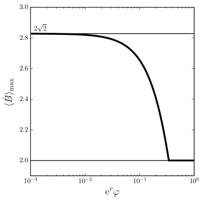
Therefore, in the large squeezing limit, all correlators depend only on a single combination of the squeezing parameters, namely $e^{r}\varphi$. In Fig. 16, the maximum Bell’s operator expectation value $\langle B\rangle_{\mathrm{max}}$ is displayed as a function of $e^{r}\varphi$, in the large squeezing limit. One can see that in this regime, Bell’s inequalities violation can be realized if and only if

$$e^{r}\varphi<0.34\,.$$ (179)

This is why in Fig. 5, the line $\varphi=0.34\,e^{-r}$ has been displayed, and one can check that when $r\gtrsim 3$, this line accurately delimits the region where Bell’s inequality violation occurs. Moreover, we also verify that all isocolor lines are indeed aligned with it. Finally, let us note that the two asymptotic regimes of Fig. 16 can be understood as follows. When $e^{r}\varphi\gg 1$, $\gamma_{3}^{2}/\gamma_{1}\gg 1$ hence $\langle\hat{S}_{x}\hat{S}_{x}\rangle\ll 1$ in Eq. (177) [one can also show that $\langle\hat{S}_{z}\hat{S}_{z}\rangle\ll 1$ in Eq. (160)] and no Bell’s inequality violation can be realized. In the opposite limit when $e^{r}\varphi\ll 1$, one can take $\gamma_{3}^{2}/\gamma_{1}\simeq 0$ in Eq. (177) and the limit $\gamma_{2}\gg 1$ can also be performed. This leads to $u(x)\simeq|x|$. Then, in the sum of Eq. (160), only the term $q=0$ gives a non vanishing contribution, and since $\vartheta_{4}(0,e^{-a})\simeq 1$ when $a\gg 1$, one obtains $\langle\hat{S}_{z}\hat{S}_{z}\rangle\simeq 1$. In the same manner, the only non vanishing term of the sum in Eq. (177) is the one for which $q=0$, yielding $\langle\hat{S}_{x}\hat{S}_{x}\rangle\simeq 1$. This is why Bell’s inequality is maximally violated in this limit.

Appendix E The Dual Case $\varphi\simeq\pi/2$

The strict validity regime of the generic approximation scheme developed in Sec. C requires that, in the large squeezing limit, the squeezing angle $\varphi$ is not too close to $\pi/2$, see Eq. (128). This condition notably ensured that $\gamma_{1}\ll 1$. In the opposite regime, where

$$r\gg 1\quad\mathrm{and}\quad\cos\varphi\ll e^{-r}\,,$$ (180)

one has $\gamma_{1}\simeq 1/(e^{-2r}+e^{2r}\cos^{2}\varphi)\gg 1$, $\gamma_{2}\simeq 2e^{-2r}\ll 1$ and $\gamma_{3}\simeq 1/\gamma_{4}\simeq-\tan\varphi\ll-1$, and the approximation scheme of Sec. C does not apply.

However, as noticed in Sec. A, the two situations are dual and connected through the formulas (71)-(73). Therefore, for any configuration such that $\varphi\simeq\pi/2$, one can always study the dual configuration for which $\varphi\simeq 0$ making use of the approximation scheme of Sec. C, and then use Eqs. (71)-(73) to obtain all correlation functions [in particular, from Eq. (20), it is clear that the expectation value of the Bell operator is the same in the two dual configurations].

Notwithstanding, in this section we develop an approximation scheme specific to configurations such that $\varphi\simeq\pi/2$. The reason is that, as one will see, such a scheme relies on a completely different technique from the one used in Sec. A, namely saddle-point approximations. Such methods may be preferred, notably since they easily allow one to go to arbitrarily higher order in the approximation, something which is not possible with the scheme of Sec. A. Therefore, if one wanted to compute higher order corrections of the results of Sec. A in the case $\varphi\simeq 0$, one would simply have to study the dual configuration when $\varphi\simeq\pi/2$ and make use of the saddle-point techniques developed in this section. In this work, we therefore provide two alternative approximation schemes, and for any configuration, one can use one or the other, depending on convenience or aimed accuracy. In this section, the leading order of the approximation is derived only (and it will be checked that it leads to maximal Bell’s inequality violation, in agreement with what was noticed at the end of Sec. D for the dual configuration), but generalization to higher order can directly be obtained.

E.1 Correlation Function $\langle\Psi_{2\,{\rm sq}}|\hat{S}^{(1)}_{z}(\ell)\hat{S}^{(2)}_{z}(\ell)|\Psi_{2\,{\rm sq}}\rangle$

Let us first work out $\langle\Psi_{2\,{\rm sq}}|\hat{S}^{(1)}_{z}(\ell)\hat{S}^{(2)}_{z}(\ell)|\Psi_{2\,{\rm sq}}\rangle$ in the regime of Eq. (180). After performing the change of integration variable $x=z+n+m$, Eq. (35) can be rewritten as

$$Z^{(1)}_{n,m}=\frac{\ell}{2}\sqrt{\frac{\pi}{\gamma_{2}}}\int_{p}^{p+1}\mathrm{d}xe^{\gamma_{1}g(x)}f(x)\,,$$ (181)

where

$$f(x)=\operatorname{erf}\left[\sqrt{\gamma_{2}}\frac{\ell}{2}\left(x-p-q\right)\right]+\operatorname{erf}\left[\sqrt{\gamma_{2}}\frac{\ell}{2}\left(x-p+q\right)\right]\,,\quad\quad g(x)=-\frac{\ell^{2}}{4}x^{2}\,,$$ (182)

and where one recalls that $p=n+m$ and $q=n-m$. Since $\gamma_{1}\gg 1$ appears in the exponential argument of Eq. (181), as discussed before, the idea is to treat this expression with a saddle-point approximation. Within the integration domain, the function $g(x)$ is always maximal at one of the integral boundaries, that we denote $x_{0}$. If $p\geq 0$, one has $x_{0}=p$, while if $p<0$, then $x_{0}=p+1$. Let us now perform the change of integration variable $x=x_{0}+y/\sqrt{\gamma_{1}}$. One obtains

$$Z^{(1)}_{n,m}=\frac{\ell}{2}\sqrt{\frac{\pi}{\gamma_{2}\gamma_{1}}}\int_{\sqrt{\gamma_{1}}(p-x_{0})}^{\sqrt{\gamma_{1}}(p+1-x_{0})}\mathrm{d}ye^{\gamma_{1}g(y)}f(y)\,.$$ (183)

Since $\gamma_{1}\gg 1$, the integral is dominated by its contribution close to $y\simeq 0$ and one can expand the function $f(y)$ at first order in $1/\sqrt{\gamma_{1}}$,

$$f(y)= \operatorname{erf}\left[\sqrt{\gamma_{2}}\frac{\ell}{2}\left(x_{0}-p-q\right)\right]+\operatorname{erf}\left[\sqrt{\gamma_{2}}\frac{\ell}{2}\left(x_{0}-p+q\right)\right]+\sqrt{\frac{\gamma_{2}}{\gamma_{1}\pi}}\ell\left[e^{-\frac{\gamma_{2}}{4}\ell^{2}\left(x_{0}-p-q\right)^{2}}+e^{-\frac{\gamma_{2}}{4}\ell^{2}\left(x_{0}-p+q\right)^{2}}\right]y+\mathcal{O}\left(\frac{1}{\gamma_{1}}\right)\,.$$ (184)

The integral can then be performed exactly. If $p\geq 0$, $x_{0}=p$ and the first term of the above expansion vanishes. One then has

$$\left.f(y)\right|_{p\geq 0}= 2\sqrt{\frac{\gamma_{2}}{\gamma_{1}\pi}}\ell e^{-\frac{\gamma_{2}}{4}\ell^{2}q^{2}}y+\mathcal{O}\left(\frac{1}{\gamma_{1}}\right)\,,$$ (185)

from which it follows that

$$\left.Z^{(1)}_{n,m}\right|_{p\geq 0} =\frac{\ell^{2}}{\gamma_{1}}e^{-\frac{\gamma_{2}}{4}\ell^{2}q^{2}}\int_{0}^{\sqrt{\gamma_{1}}}e^{-\frac{\gamma_{1}\ell^{2}}{4}\left(p+\frac{y}{\sqrt{\gamma_{1}}}\right)^{2}}y\mathrm{d}y\simeq\begin{cases}\displaystyle\frac{4}{\ell^{2}p^{2}\gamma_{1}^{2}}e^{-\left(\gamma_{1}p^{2}+\gamma_{2}q^{2}\right)\frac{\ell^{2}}{4}}&\mathrm{if}\ p>0\\ \displaystyle\frac{2}{\gamma_{1}}e^{-\gamma_{2}q^{2}\frac{\ell^{2}}{4}}&\mathrm{if}\ p=0\end{cases}\,,$$ (186)

where in the second line, we have expanded the result at leading order in $1/\sqrt{\gamma_{1}}$. If $p<0$, $x_{0}=p+1$ and one has

$$f(y)=\operatorname{erf}\left[\sqrt{\gamma_{2}}\frac{\ell}{2}\left(1-q\right)\right]+\operatorname{erf}\left[\sqrt{\gamma_{2}}\frac{\ell}{2}\left(1+q\right)\right]+\mathcal{O}\left(\frac{1}{\sqrt{\gamma_{1}}}\right)\,,$$ (187)

from which one obtains

$$\left.Z^{(1)}_{n,m}\right|_{p<0} =\frac{\ell}{2}\sqrt{\frac{\pi}{\gamma_{1}\gamma_{2}}}\left\{\operatorname{erf}\left[\sqrt{\gamma_{2}}\frac{\ell}{2}\left(1-q\right)\right]+\operatorname{erf}\left[\sqrt{\gamma_{2}}\frac{\ell}{2}\left(1+q\right)\right]\right\}\int_{-\sqrt{\gamma_{1}}}^{0}\mathrm{d}ye^{-\gamma_{1}\frac{\ell^{2}}{4}\left(p+1+\frac{y}{\sqrt{\gamma_{1}}}\right)^{2}}$$ (188)

$$\simeq\begin{cases}\displaystyle-\frac{1}{\ell\gamma_{1}(p+1)}\sqrt{\frac{\pi}{\gamma_{2}}}\left\{\operatorname{erf}\left[\sqrt{\gamma_{2}}\frac{\ell}{2}\left(1-q\right)\right]+\operatorname{erf}\left[\sqrt{\gamma_{2}}\frac{\ell}{2}\left(1+q\right)\right]\right\}e^{-\gamma_{1}(p+1)^{2}}\frac{\ell^{2}}{4}&\mathrm{if}\ p<-1\\ \displaystyle\frac{\pi}{2\sqrt{\gamma_{1}\gamma_{2}}}\left\{\operatorname{erf}\left[\sqrt{\gamma_{2}}\frac{\ell}{2}\left(1-q\right)\right]+\operatorname{erf}\left[\sqrt{\gamma_{2}}\frac{\ell}{2}\left(1+q\right)\right]\right\}&\mathrm{if}\ p=-1\end{cases}\,,$$ (189)

where in the second line, we have again expanded the result at leading order in $1/\sqrt{\gamma_{1}}$. From these expressions, it is clear that the terms such that $p>0$ or $p<-1$ are exponentially suppressed in the limit $\gamma_{1}\gg 1$. In some sense, the situation is similar to the one of the large $\ell$ limit, see Sec. B.1, since only the terms $p=0$ and $p=-1$ give a non-negligible contribution. Recalling that $p$ and $q$ must have same parity, one then has

$$\sum_{n,m=-\infty}^{\infty}(-1)^{n+m}Z_{n,m}^{(1)}=\frac{2}{\gamma_{1}}\sum_{q\,\mathrm{even}}e^{-\gamma_{2}\ell^{2}q^{2}/4}-\frac{\pi}{2\sqrt{\gamma_{1}\gamma_{2}}}\sum_{q\,\mathrm{odd}}\left\{\operatorname{erf}\left[\sqrt{\gamma_{2}}\frac{\ell}{2}(1-q)\right]+\operatorname{erf}\left[\sqrt{\gamma_{2}}\frac{\ell}{2}\left(q+1\right)\right]\right\}\,.$$ (190)

It is now time to make use of the fact that, in the regime under consideration, $\gamma_{2}\ll 1$. In this limit, the second error function can be expanded around the argument of the first one, and one obtains

$$\sum_{n,m=-\infty}^{\infty}(-1)^{n+m}Z_{n,m}^{(1)}\simeq\frac{2}{\gamma_{1}}\sum_{q=-\infty}^{\infty}e^{-\gamma_{2}\ell^{2}q^{2}}-\sqrt{\frac{\pi}{\gamma_{1}}}\ell\sum_{q=-\infty}^{\infty}e^{-\gamma_{2}\ell^{2}q^{2}}\,.$$ (191)

It is interesting to notice that the first term, corresponding to $p=0$, is subdominant at leading order in $1/\sqrt{\gamma_{1}}$, which is consistent with the fact that the leading term in Eq. (184) vanishes for $p\geq 0$ and $x_{0}=p$. One then obtains

$$\sum_{n,m=-\infty}^{\infty}(-1)^{n+m}Z_{n,m}^{(1)}\simeq-\sqrt{\frac{\pi}{\gamma_{1}}}\ell\vartheta_{3}\left(0,e^{-\gamma_{2}\ell^{2}}\right)\simeq-\frac{\pi}{\sqrt{\gamma_{1}\gamma_{2}}}\,,$$ (192)

where we have expanded the final result in the $\gamma_{2}\ll 1$ limit. Making use of Eq. (37), this gives rise to

$$\langle\Psi_{2\,{\rm sq}}|\hat{S}^{(1)}_{z}(\ell)\hat{S}^{(2)}_{z}(\ell)|\Psi_{2\,{\rm sq}}\rangle=-1\,.$$ (193)

This is in agreement with Eq. (71) and the limit derived at the very end of Sec. D.

E.2 Correlation Functions $\langle\Psi_{2\,{\rm sq}}|\hat{S}^{(1)}_{x}(\ell)\hat{S}^{(2)}_{x}(\ell)|\Psi_{2\,{\rm sq}}\rangle$ and $\langle\Psi_{2\,{\rm sq}}|\hat{S}^{(1)}_{y}(\ell)\hat{S}^{(2)}_{y}(\ell)|\Psi_{2\,{\rm sq}}\rangle$

Let us now make use of the same technique to calculate the correlation function of the $x$ and $y$-components of the spin operators. Let us start with the term $X_{n,m}^{(1)}$ given by Eq. (A.2), our goal being to put this expression under a form similar to Eq. (181). Straightforward manipulations lead to

$$X^{(1)}_{n,m}=e^{-\gamma_{1}\ell^{2}/2}\ell\sqrt{\frac{\pi}{\gamma_{2}}}\int_{2p}^{2p+1}\mathrm{d}xe^{\gamma_{1}g(x)}f(x)\,,$$ (194)

where, now, the functions $f(x)$ and $g(x)$ are defined by

$$f(x)=\cos\left[\gamma_{3}\ell^{2}\left(x+1\right)\right]\left\{\operatorname{erf}\left[\sqrt{\gamma_{2}}\frac{\ell}{2}\left(x-2p-2q\right)\right]+\operatorname{erf}\left[\sqrt{\gamma_{2}}\frac{\ell}{2}\left(x-2p+2q\right)\right]\right\}\,,\quad g(x)=-\frac{\ell^{2}}{4}x(x+2)\,.$$ (195)

Then, the calculation proceeds exactly in the same way as before. The integral is dominated by contributions coming from the point $x_{0}$ with $x_{0}=2p$ when $p\geq 0$ and $x_{0}=2p+1$ when $p<-1$. One then write $x=x_{0}+y/\sqrt{\gamma_{1}}$ and expands the results in inverse powers of $\gamma_{1}$. Notice that, at leading order, the cosine function present in $f(x)$ never contributes since the corresponding first correction is quadratic in $x$. For $x_{0}=2p$, one obtains

$$\left.X_{n,m}^{(1)}\right|_{p\geq 0}\simeq\frac{8}{\gamma_{1}^{2}\ell^{2}(1+2p)^{2}}\cos\left[\gamma_{3}\ell^{2}\left(2p+1\right)\right]e^{-\gamma_{2}\ell^{2}q^{2}}e^{-\gamma_{1}\ell^{2}(1+2p+2p^{2})/2}.$$ (196)

Notice that this expression is perfectly valid when $p=0$ contrary to the corresponding case for the $z$-component spin correlation function. In the case $x_{0}=2p+1$, similar considerations lead to

$$\left.X^{(1)}_{n,m}\right|_{p<-1} \simeq-\frac{e^{-\gamma_{1}\ell^{2}/2}}{\ell\gamma_{1}(p+1)}\sqrt{\frac{\pi}{\gamma_{2}}}\cos\left[\gamma_{3}\ell^{2}\left(2p+2\right)\right]\left\{\operatorname{erf}\left[\sqrt{\gamma_{2}}\frac{\ell}{2}\left(1-q\right)\right]+\operatorname{erf}\left[\sqrt{\gamma_{2}}\frac{\ell}{2}\left(1+q\right)\right]\right\}e^{-\gamma_{1}\ell^{2}(1+2p)(3+2p)/4}\,,$$ (197)

while, if $p=-1$, one has

$$\left.X^{(1)}_{n,m}\right|_{p=-1}\simeq 2\ell\sqrt{\frac{\pi}{\gamma_{1}}}e^{-\gamma_{1}\ell^{2}/4-\gamma_{2}\ell^{2}q^{2}}\,,$$ (198)

It is clear that $p=-1$ gives the dominant contribution. The term corresponding to $p=0$ is not exponentially killed but contains additional power of $\gamma_{1}$ at the denominator. Therefore, it can be discarded. Then, in order to calculate the first sum, we just have to perform the sum over $q$ in the previous equation which can be done, as usual, in terms of a Jacobi function. Using that $\gamma_{2}\ll 1$, one arrives at

$$\sum_{n,m=-\infty}^{\infty}X_{n,m}^{(1)}\simeq\frac{\pi}{\sqrt{\gamma_{1}\gamma_{2}}}e^{-\gamma_{1}\ell^{2}/4}.$$ (199)

The calculation of $X_{n,m}^{(2)}$ proceeds along the same lines, the only (slightly) more complicated aspect being that one has now to deal with complex error functions. Working out Eq. (63), one arrives at

$$X^{(2)}_{n,m}=e^{-(\gamma_{1}+\gamma_{2})\ell^{2}/4-\gamma_{4}^{2}/\gamma_{2}\ell^{2}}\frac{\ell}{2}\sqrt{\frac{\pi}{\gamma_{2}}}\int_{2p}^{2p+1}\mathrm{d}xe^{\gamma_{1}g(x)}f(x)\,,$$ (200)

where the functions $f(x)$ and $g(x)$ can be expressed as

$$f(x) =\biggl{\{}\operatorname{erf}\left[\sqrt{\gamma_{2}}\frac{\ell}{2}\left(x-2p-2q\right)+i\frac{\gamma_{4}}{\sqrt{\gamma_{2}}}\ell\right]+\operatorname{erf}\left[\sqrt{\gamma_{2}}\frac{\ell}{2}\left(x-2p-2q\right)-i\frac{\gamma_{4}}{\sqrt{\gamma_{2}}}\ell\right]$$

$$+\operatorname{erf}\left[\sqrt{\gamma_{2}}\frac{\ell}{2}\left(x-2p+2q\right)+i\frac{\gamma_{4}}{\sqrt{\gamma_{2}}}\right]+\operatorname{erf}\left[\sqrt{\gamma_{2}}\frac{\ell}{2}\left(x-2p+2q\right)-i\frac{\gamma_{4}}{\sqrt{\gamma_{2}}}\right]\biggr{\}}\,,$$ (201)

and $g(x)=-\ell^{2}x(x+2)/4$. As before, one must distinguish whether one deals with the case $x_{0}=2p$ or $x_{0}=2p+1$ and it is easy to convince oneself that the dominant contribution will be given by $p=-1$ for which one has

$$\left.X^{(2)}_{n,m}\right|_{p=-1}\simeq 2\ell\sqrt{\frac{\pi}{\gamma_{1}}}e^{-\gamma_{2}\ell^{2}/4-\gamma_{4}^{2}/\gamma_{2}\ell^{2}-\gamma_{2}\ell^{2}q^{2}}\,,$$ (202)

Performing the sum over $q$ is now standard and one obtains

$$\sum_{n,m=-\infty}^{\infty}X_{n,m}^{(2)}\simeq\frac{\pi}{\sqrt{\gamma_{1}\gamma_{2}}}e^{-\gamma_{2}\ell^{2}/4-\gamma_{4}^{2}/\gamma_{2}\ell^{2}}.$$ (203)

Similar considerations can be made for the two remaining integrals.

Combining these results with Eqs. (66), one finally obtains

$$\langle\Psi_{2\,{\rm sq}}|\hat{S}^{(1)}_{x}(\ell)\hat{S}^{(2)}_{x}(\ell)|\Psi_{2\,{\rm sq}}\rangle\simeq e^{-\gamma_{1}\ell^{2}/4}+e^{-\gamma_{2}\ell^{2}/4-\gamma_{4}^{2}/\gamma_{2}\ell^{2}}\simeq 1$$ (204)

where we have taken the limits $\gamma_{1}\gg 1$ and $\gamma_{2},\gamma_{4}^{2}/\gamma_{2}\ll 1$. In the same way, using Eq. (70), one has

$$\langle\Psi_{2\,{\rm sq}}|\hat{S}^{(1)}_{y}(\ell)\hat{S}^{(2)}_{y}(\ell)|\Psi_{2\,{\rm sq}}\rangle\simeq-e^{-\gamma_{1}\ell^{2}/4}+e^{-\gamma_{2}\ell^{2}/4-\gamma_{4}^{2}/\gamma_{2}\ell^{2}}\simeq 1\,.$$ (205)

These results are in agreement with Eqs. (72) and (73) and the limit derived at the very end of Sec. D. This also confirms that Bell’s inequalities are maximally violated in the large squeezing limit when $\varphi=\pi/2$.

Appendix F Rotation in Phase-Space

In this section, we investigate the situation where the pseudo-spin operators are defined with respect to a direction in phase space that is different from the position $Q$ considered in the rest of this paper. Let us therefore introduce the rotation in phase space

$$\overline{\hat{Q}}_{i} =\hat{Q}_{i}\cos\alpha-\hat{P}_{i}\sin\alpha,$$ (206)

$$\overline{\hat{P}}_{i} =\hat{P}_{i}\cos\alpha+\hat{Q}_{i}\sin\alpha,$$ (207)

where $\alpha$ is a real angle parameter and $i=1,2$. One can easily check that $[\hat{Q}_{i},\hat{P}_{i}]=[\overline{\hat{Q}}_{i},\overline{\hat{P}}_{i}]$ and this transformation is therefore canonical. As a consequence, it can be represented by a unitary operator $U_{i}$ which, in the present case, takes the following form Anderson (1994)

$$U_{i}=\exp\left[\frac{i}{2}\ln(\cos\alpha)\left(\hat{P}_{i}\hat{Q}_{i}+\hat{Q}_{i}\hat{P}_{i}\right)\right]\exp\left[\frac{i}{2}\sin(2\alpha)\hat{Q}_{i}^{2}\right]\exp\left(-\frac{i}{2}\tan\alpha\hat{P}_{i}^{2}\right).$$ (208)

One can indeed check that the transformation given by Eqs. (206) and (207) is realized by $\overline{\hat{Q}}_{i}=U_{i}\hat{Q}_{i}U_{i}^{\dagger}$ and $\overline{\hat{P}}_{i}=U_{i}\hat{P}_{i}U_{i}^{\dagger}$. The next step is to study how the state (27) transforms under this canonical transformation Moshinsky and Quesne (1971). For this purpose, let us consider the eigenstates $|Q_{i}\rangle$ and $|\overline{Q}_{i}\rangle$ of the operators $\hat{Q}_{i}$ and $\overline{\hat{Q}}_{i}$, respectively. One can sandwich Eqs. (206) and (207) between $\langle Q_{i}|$ and $|\overline{Q}_{i}\rangle$ and use the fact that $\langle Q_{i}|\hat{P}_{i}|\overline{Q}_{i}\rangle=-i\partial\langle Q_{i}|\overline{Q}_{i}\rangle/(\partial Q_{i})$ and $\langle Q_{i}|\overline{\hat{P}}_{i}|\overline{Q}_{i}\rangle=i\partial\langle Q_{i}|\overline{Q}_{i}\rangle/(\partial\overline{Q}_{i})$. This results in two differential equations that reads

$$\frac{\partial}{\partial Q_{i}}\langle Q_{i}|\overline{Q}_{i}\rangle =\frac{i}{\sin\alpha}\left(\cos\alpha Q_{i}-\overline{Q}_{i}\right)\langle Q_{i}|\overline{Q}_{i}\rangle,$$ (209)

$$\frac{\partial}{\partial\overline{Q}_{i}}\langle Q_{i}|\overline{Q}_{i}\rangle =-\frac{i}{\sin\alpha}\left(Q_{i}-\cos\alpha\overline{Q}_{i}\right)\langle Q_{i}|\overline{Q}_{i}\rangle,$$ (210)

and leads to

$$\langle Q_{i}|\overline{Q}_{i}\rangle=C\exp\left(-\frac{i}{\sin\alpha}Q_{i}\overline{Q}_{i}+\frac{i}{2\tan\alpha}Q_{i}^{2}+\frac{i}{2\tan\alpha}\overline{Q}_{i}^{2}\right),$$ (211)

where $C$ is a constant. From this expression, one can now infer the wavefunction of the system after the canonical transformation. It is given by

$$\langle\Psi_{\rm 2\,sq}|\overline{Q}_{1},\overline{Q}_{2}\rangle\equiv\Psi_{\rm 2\,sq}\left(\overline{Q}_{1},\overline{Q}_{2}\right)=\int\langle\Psi|Q_{1},Q_{2}\rangle\langle Q_{1}|\overline{Q}_{1}\rangle\langle Q_{2}|\overline{Q}_{2}\rangle{\rm d}Q_{1}{\rm d}Q_{2},$$ (212)

where $\langle\Psi_{\rm 2\,sq}|Q_{1},Q_{2}\rangle=\Psi_{\rm 2\,sq}\left(Q_{1},Q_{2}\right)\propto e^{A\left(Q_{1}^{2}+Q_{2}^{2}\right)-BQ_{1}Q_{2}}$ is given by Eq. (27). This integral can easily be performed since it is a Gaussian integral. Concretely, one has

$$\Psi_{\rm 2\,sq}\left(\overline{Q}_{1},\overline{Q}_{2}\right)\propto e^{i(\overline{Q}_{1}^{2}+\overline{Q}_{2}^{2})/(2\tan\alpha)}\int e^{-{\bf Q}^{\rm T}M{\bf Q}/2-{\bf J}^{\rm T}{\bf Q}}{\rm d}Q_{1}{\rm d}Q_{2},$$ (213)

where

$${\bf Q}=\begin{pmatrix}Q_{1}\\ Q_{2}\end{pmatrix},\quad{\bf J}=\frac{i}{\sin\alpha}\begin{pmatrix}\overline{Q}_{1}\\ \overline{Q}_{2}\end{pmatrix},\quad M=\begin{pmatrix}-2A-\frac{i}{\tan\alpha}&B\\ B&-2A-\frac{i}{\tan\alpha}\end{pmatrix},$$ (214)

and straightforward calculations leads to

$$\Psi_{\rm 2\,sq}\left(\overline{Q}_{1},\overline{Q}_{2}\right)\propto e^{i(\overline{Q}_{1}^{2}+\overline{Q}_{2}^{2})/(2\tan\alpha)}e^{{\bf J}^{\rm T}M^{-1}{\bf J}/2}=e^{\overline{A}\left(\overline{Q}_{1}^{2}+\overline{Q}_{2}^{2}\right)-\overline{B}\,\overline{Q}_{1}\overline{Q}_{2}},$$ (215)

where the new quantities $\overline{A}$ and $\overline{B}$ can be expressed as

$$\overline{A} =\frac{i}{2\tan\alpha}+\frac{1}{2\sin^{2}\alpha\det M}\left(2A+\frac{i}{\tan\alpha}\right)=A(r,\varphi+\alpha)$$ (216)

$$\overline{B} =-\frac{B}{\sin^{2}\alpha\det M}=B(r,\varphi+\alpha).$$ (217)

We conclude that, after the rotation, the wavefunction keeps its shape unmodified, the squeezing parameter also remains unchanged but the squeezing angle becomes $\varphi+\alpha$.

Interestingly enough, the above result can also be established directly in phase space. A convenient tool to carry out this calculation is the Wigner function Wigner (1932); Case (2008)

$$W_{\rm 2\,sq}(Q_{1},P_{1},Q_{2},P_{2})=\frac{1}{\left(2\pi\right)^{2}}\int\mathrm{d}x\mathrm{d}y\Psi_{\rm 2\,sq}^{*}\left(Q_{1}-\frac{x}{2},Q_{2}-\frac{y}{2}\right)e^{-iP_{1}x-iP_{2}y}\Psi_{\rm 2\,sq}\left(Q_{1}+\frac{x}{2},Q_{2}+\frac{y}{2}\right),$$ (218)

which is a quasiprobability distribution in phase space that provides an equivalent description of the quantum state than that of the wavefunction or the density matrix. For the two-mode squeezed state (27), Gaussian integration leads to Case (2008); Martin and Vennin (2016a)

$$W_{\rm 2\,sq}(Q_{1},P_{1},Q_{2},P_{2})=\frac{1}{\pi^{2}}\exp \left[-\cosh(2r)\left(Q_{1}^{2}+Q_{2}^{2}+P_{1}^{2}+P_{2}^{2}\right)+2\sinh(2r)\sin(2\varphi)\left(Q_{1}P_{2}+Q_{2}P_{1}\right)\right.$$

$$\left.+2\sinh(2r)\cos(2\varphi)\left(Q_{1}Q_{2}-P_{1}P_{2}\right)\right]\,.$$ (219)

If one replaces $Q_{i}$ and $P_{i}$ by their expressions (206) and (207) in terms of $\overline{Q}_{i}$ and $\overline{P}_{i}$ in this formula, one directly obtains

$$W_{\rm 2\,sq}(\overline{Q}_{1},\overline{P}_{1},\overline{Q}_{2},\overline{P}_{2})=\frac{1}{\pi^{2}}\exp \left\{-\cosh(2r)\left(\overline{Q}_{1}^{2}+\overline{Q}_{2}^{2}+\overline{P}_{1}^{2}+\overline{P}_{2}^{2}\right)+2\sinh(2r)\sin\left[2\left(\varphi+\alpha\right)\right]\left(\overline{Q}_{1}\overline{P}_{2}+\overline{Q}_{2}\overline{P}_{1}\right)\right.$$

$$\left.+2\sinh(2r)\cos\left[2\left(\varphi+\alpha\right)\right]\left(\overline{Q}_{1}\overline{Q}_{2}-\overline{P}_{1}\overline{P}_{2}\right)\right\}\,.$$ (220)

Comparing with Eq. (219), one notices that the same Wigner function is obtained, except that the squeezing angle has been redefined according to $\varphi\rightarrow\varphi+\alpha$. The wavefunction in the $\overline{Q}$-position representation is therefore given by the same expression as Eq. (27), if one replaces $\varphi$ by $\varphi+\alpha$, which is exactly the result we have obtained previously.

As a consequence, if one defines the pseudo-spin operators with respect to $\overline{Q}$ instead of $Q$, that is to say, if one replaces $Q$ by $\overline{Q}$ everywhere in Eqs. (1)-(9), then one obtains the same results as the ones derived above except that $\varphi$ must be replaced by $\varphi+\alpha$. The analysis presented in this paper therefore allows one to deal with any orientation between the squeezing angle of the wavefunction and the pseudo-spin operators.

References

- Bell (1964) J. S. Bell, Physics 1, 195 (1964).
- Aspect et al. (1982a) A. Aspect, P. Grangier, and G. Roger, Phys. Rev. Lett. 49, 91 (1982a).
- Aspect et al. (1982b) A. Aspect, J. Dalibard, and G. Roger, Phys. Rev. Lett. 49, 1804 (1982b).
- Weihs et al. (1998) G. Weihs, T. Jennewein, C. Simon, H. Weinfurter, and A. Zeilinger, Phys. Rev. Lett. 81, 5039 (1998), eprint quant-ph/9810080.
- Hensen et al. (2015) B. Hensen et al., Nature 526, 682 (2015), eprint 1508.05949.
- Einstein et al. (1935) A. Einstein, B. Podolsky, and N. Rosen, Phys. Rev. 47, 777 (1935).
- Clauser et al. (1969) J. F. Clauser, M. A. Horne, A. Shimony, and R. A. Holt, Phys. Rev. Lett. 23, 880 (1969).
- Larsson (2004) J.-Å. Larsson, Phys. Rev. A 70, 022102 (2004), eprint quant-ph/0310140.
- Chen et al. (2002) Z.-B. Chen, J.-W. Pan, G. Hou, and Y.-D. Zhang, Phys. Rev. Lett. 88, 040406 (2002).
- Yarnall et al. (2007) T. Yarnall, A. F. Abouraddy, B. E. A. Saleh, and M. C. Teich, Phys. Rev. Lett. 99, 170408 (2007).
- Larsson (2003) J.-Å. Larsson, Phys. Rev. A 67, 022108 (2003), eprint quant-ph/0208125.
- Brukner et al. (2003) Č. Brukner, M. S. Kim, J.-W. Pan, and A. Zeilinger, Phys. Rev. A 68, 062105 (2003), eprint quant-ph/0208116.
- Dorantes and Lucio M (2009) M. M. Dorantes and J. L. Lucio M, Journal of Physics A Mathematical General 42, 285309 (2009).
- Henderson and Vedral (2001) L. Henderson and V. Vedral (2001), eprint 0105028.
- Ollivier and Zurek (2001) H. Ollivier and W. H. Zurek, Phys. Rev. Lett. 88, 017901 (2001).
- Martin and Vennin (2016a) J. Martin and V. Vennin, Phys. Rev. D93, 023505 (2016a), eprint 1510.04038.
- Schwinger (1951) J. S. Schwinger, Phys. Rev. 82, 664 (1951).
- Starobinsky (1979) A. A. Starobinsky, JETP Lett. 30, 682 (1979).
- Starobinsky (1980) A. A. Starobinsky, Phys. Lett. B91, 99 (1980).
- Sato (1981) K. Sato, Mon. Not. Roy. Astron. Soc. 195, 467 (1981).
- Guth (1981) A. H. Guth, Phys. Rev. D23, 347 (1981).
- Linde (1982) A. D. Linde, Phys. Lett. B108, 389 (1982).
- Mukhanov and Chibisov (1981) V. F. Mukhanov and G. Chibisov, JETP Lett. 33, 532 (1981).
- Albrecht and Steinhardt (1982) A. Albrecht and P. J. Steinhardt, Phys. Rev. Lett. 48, 1220 (1982).
- Hawking (1982) S. Hawking, Phys. Lett. B115, 295 (1982).
- Starobinsky (1982) A. A. Starobinsky, Phys. Lett. B117, 175 (1982).
- Guth and Pi (1982) A. H. Guth and S. Pi, Phys. Rev. Lett. 49, 1110 (1982).
- Bardeen et al. (1983) J. M. Bardeen, P. J. Steinhardt, and M. S. Turner, Phys. Rev. D28, 679 (1983).
- Linde (1983) A. D. Linde, Phys. Lett. B129, 177 (1983).
- Martin (2005a) J. Martin, Int. J. Mod. Phys. A20, 4676 (2005a), eprint astro-ph/0410629.
- Martin (2005b) J. Martin, Lect. Notes Phys. 669, 199 (2005b), eprint hep-th/0406011.
- Martin (2004) J. Martin, Braz. J. Phys. 34, 1307 (2004), eprint astro-ph/0312492.
- Martin (2013) J. Martin, in Rencontres du Vietnam: Hot Topics in General Relativity and Gravitation Quy Nhon, Vietnam, 28 July—3 August 2013 (2013), eprint 1312.3720.
- Vennin et al. (2015) V. Vennin, J. Martin, and C. Ringeval, Comptes Rendus Physique (2015).
- Martin (2015) J. Martin (2015), eprint 1502.05733.
- Grishchuk and Sidorov (1990) L. Grishchuk and Y. Sidorov, Phys. Rev. D42, 3413 (1990).
- Martin (2008) J. Martin, Lect. Notes Phys. 738, 193 (2008), eprint 0704.3540.
- Martin and Vennin (2016b) J. Martin and V. Vennin, In preparation. (2016b).
- Martin et al. (2012) J. Martin, V. Vennin, and P. Peter, Phys. Rev. D86, 103524 (2012), eprint 1207.2086.
- Martin (2012) J. Martin, J. Phys. Conf. Ser. 405, 012004 (2012), eprint 1209.3092.
- Cirel’Son (1980) B. S. Cirel’Son, Letters in Mathematical Physics 4, 93 (1980).
- Fixsen et al. (1996) D. J. Fixsen, E. S. Cheng, J. M. Gales, J. C. Mather, R. A. Shafer, and E. L. Wright, Astrophys. J. 473, 576 (1996), eprint astro-ph/9605054.
- Bell (1987) J. S. Bell, Speakable and unspeakable in quantum mechanics. Collected papers on quantum philosophy (1987).
- Gour et al. (2004) G. Gour, F. C. Khanna, A. Mann, and M. Revzen, Physics Letters A 324, 415 (2004), eprint quant-ph/0308063.
- Revzen et al. (2005) M. Revzen, P. A. Mello, A. Mann, and L. M. Johansen, Phys. Rev. A 71, 022103 (2005), eprint quant-ph/0405100.
- Revzen (2006) M. Revzen, Foundations of Physics 36, 546 (2006).
- Lundeen et al. (2011) J. S. Lundeen, B. Sutherland, A. Patel, C. Stewart, and C. Bamber, ArXiv e-prints (2011), eprint 1112.3575.
- Gradshteyn and Ryzhik (1965) I. S. Gradshteyn and I. M. Ryzhik, Table of Integrals, Series, and Products (Academic Press, New York and London, 1965).
- Anderson (1994) A. Anderson, Annals of Physics 232, 292 (1994), eprint hep-th/9305054.
- Moshinsky and Quesne (1971) M. Moshinsky and C. Quesne, Journal of Mathematical Physics 12, 1772 (1971).
- Wigner (1932) E. Wigner, Physical Review 40, 749 (1932).
- Case (2008) W. B. Case, Am. J. Phys. 76, 937 (2008).