Retrieving the Covariance Matrix of an Unknown Two-Mode Gaussian State by Means of a Reference Twin Beam

Abstract

A method for revealing the covariance matrix of an unknown two-mode Gaussian state is given based on the interference with a reference twin beam whose covariance matrix is known. In the method, first- and second-order cross-correlation intensity moments are determined varying the overall phase of the reference twin beam.

1 Introduction

The reconstruction of a state of any quantum system belongs to the most important tasks in quantum physics [1, 2, 3]. For this reason, homodyne detection has been suggested and experimentally implemented for the first time in Ref. [4] for quantum light. This was the first successful example of the so-called quantum state tomography, that provides the full information about the analyzed quantum state. The knowledge of the quantum state of light is extraordinarily important, as such states are useful for testing the postulates of quantum mechanics, showing peculiar features of quantum states (teleportation [5], dense coding [6, 7], etc.), as well as applying them in metrology and other applications (cryptography [8, 9]).

The optical homodyne tomography both in its cw and pulsed variants has become the most advanced and also powerful method in quantum state tomography [10] and, as such, it has become an indispensable technique in the field of quantum optics. The method is based upon overlapping an unknown state with a classical light (coherent state) with a well-defined phase, that is called a local oscillator. The interference pattern depending on the varying phase of the local oscillator then allows to reconstruct the quantum state, in detail to reconstruct its Wigner function defined in the phase space  [1, 10]. Subsequently, moments of the field operators can be obtained and used to fully characterize nonclassicality of the analyzed quantum state [11, 12]. However, the optical homodyne tomography is quite experimentally involved and requires extended experimental data sets [10].

For this reason, a simplified method still relying on the coherent local oscillator has been suggested for quantum state tomography in [13], and later elaborated in [14, 15]. In this method, one of the output ports of a beam splitter that mixes the analyzed light with the local oscillator is monitored in general by a photon-number resolving detector with the varying attenuation coefficient. Also an attempt to use the data measured under different levels of noise for quantum state tomography has been made [16].

In many cases, the light to be analyzed has specific properties that allow to apply simpler tools in the determination of its state. For example, when we analyze the properties of twin beams generated from the vacuum state by parametric down-conversion [17], the characterization by means of the measured photocount statistics is fully sufficient [18, 19]. This possibility originates in the generation process that does not ‘prescribe’ specific phases to the individual signal and idler fields. Here, the generated light is Gaussian without coherent components, i.e. it is completely characterized by means of its covariance matrix. Once the covariance matrix of a given state is obtained, all the properties of the state are easily derived. As useful examples, entanglement of a two-mode twin beam or local nonclassicalities of one-mode reduced states can be mentioned [20]. Even phase-space quasidistributions of integrated intensities can be determined [21].

Whereas the analysis of covariance matrices of Gaussian two-mode twin beams is not difficult since only certain elements of their covariance matrices are nonzero, the measurement of covariance matrices belonging to a general two-mode Gaussian state is more involved. To cope with this problem, we have developed a method for reconstructing the normally- or symmetrically-ordered covariance matrix of such a general two-mode Gaussian state based on mixing the analyzed state with a reference twin beam with the varying overall phase.

Moreover, the developed approach can be extended to multimode Gaussian states provided that the measurement on individual mode pairs can be performed. This is useful, e.g., for spectrally multimode twin beams composed of $N$ paired modes. Even in this case, the genuine multimode entanglement of the state can be retrieved from its multimode covariance matrix [22, 23]. A specific example of this general approach was studied by Altepeter et al. [24] who reconstructed the polarization state of a photon pair by acquiring photon coincidence-count statistics.

The paper is organized as follows. Description of general two-mode Gaussian states through their covariance matrices is given in Sec. II. Twin beams as the most common kind of two-mode Gaussian states are discussed in Sec. III. The method for revealing the covariance matrix of a general two-mode Gaussian state is given in Sec. IV. Sec. V brings conclusions.

2 General two-mode Gaussian states

The normally-ordered characteristic function $C_{\mathcal{N}}$ for a general two-mode Gaussian state is defined as follows

$$C_{\mathcal{N}}(\beta_{1},\beta_{2})=\mathrm{Tr}\left[\hat{\rho}(0)\exp(\beta_{1}\hat{a}^{\dagger}_{1}+\beta_{2}\hat{a}^{\dagger}_{2})\exp(-\beta^{\ast}_{1}\hat{a}_{1}-\beta^{\ast}_{2}\hat{a}_{2})\right],$$ (1)

where Tr stands for the operator trace and $\hat{a}_{i}$ ($\hat{a}_{i}^{\dagger}$) denote the boson annihilation (creation) operators of mode $i$, $i=1,2$.

The normally-ordered characteristic function $C_{\mathcal{N}}$ in Eq. (1) can be expressed via its complex covariance matrix ${\bf A}_{\cal N}$,

$${\bf A}_{\cal N}=\left[\begin{array}[]{cc}{\bf B}_{1}&{\bf D}_{12}\cr{\bf D}_{12}^{\dagger}&{\bf B}_{2}\end{array}\right],$$ (4)

$$\hskip 14.22636pt{\bf B}_{j}=\left[\begin{array}[]{cc}-B_{j}&C_{j}\cr C_{j}^{*}&-B_{j}\end{array}\right],\hskip 8.53581ptj=1,2,\hskip 8.53581pt{\bf D}_{12}=\left[\begin{array}[]{cc}\bar{D}_{12}^{*}&{D}_{12}\cr{D}_{12}^{*}&\bar{D}_{12}\end{array}\right],$$ (9)

in the form $C_{\cal N}(\hat{\mbox{\boldmath$\beta$}})=\exp(\hat{\mbox{\boldmath$\beta$}}^{\dagger}{\bf A}_{\mathcal{N}}\hat{\mbox{\boldmath$\beta$}}/2)$, where $\hat{\mbox{\boldmath$\beta$}}=(\beta_{1},\beta_{1}^{\ast},\beta_{2},\beta_{2}^{\ast})^{T}$. The coefficients $B_{j}$, $C_{j}$, $j=1,2$, $\bar{D}_{12}$ and $D_{12}$ occurring in Eq. (4) are defined as

$$B_{j}=\langle\Delta\hat{a}^{\dagger}_{j}\Delta\hat{a}_{j}\rangle, C_{j}=\langle\Delta\hat{a}_{j}^{2}\rangle,$$

$$D_{12}=\langle\Delta\hat{a}_{1}\Delta\hat{a}_{2}\rangle, \bar{D}_{12}=-\langle\Delta\hat{a}_{1}^{\dagger}\Delta\hat{a}_{2}\rangle.$$ (10)

The determination of coefficients $B_{j}$ and $C_{j}$, $j=1,2$, together with the coefficients $D_{12}$ and $\bar{D}_{12}$ is thus sufficient to fully characterize a general two-mode Gaussian field without coherent components. All possible correlation functions can then be easily derived [17].

The coefficients occurring in the normally-ordered covariance matrix $\bf A_{\mathcal{N}}$ give also the coefficients in the symmetrically-ordered covariance matrix $\bf A_{\mathcal{S}}$ [25], which is important for the determination of entanglement. Indeed, the determinant $I_{4}\equiv{\rm det}(\bf A_{\mathcal{S}})$ of the symmetrically-ordered covariance matrix along with the local unitary invariants $I_{j}$, $j=1,2,3,$ and $I_{j\mathcal{S}}$, $j=1,2$ of the normally- and symmetrically-ordered covariance matrices, respectively, completely quantify both nonclassicality and entanglement of the state (for details, see [20]).

3 Pure twin beams

To determine the needed coefficients, we use as a reference a pure twin beam with a specific form of its covariance matrix. Pure twin beams represent a specific form of two-mode Gaussian states that is standardly generated in the process of parametric down-conversion. The boson operators characterizing the emitted signal ($\hat{a}_{1}^{\rm out}$) and idler ($\hat{a}_{2}^{\rm out}$) fields are written in the Heisenberg picture as follows [17]:

$$\hat{a}_{1}^{\rm out} = \cosh(\sqrt{G})\hat{a}_{1}^{\rm in}+i\exp(i\phi)\sinh(\sqrt{G})\hat{a}_{2}^{{\rm in}\dagger},$$

$$\hat{a}_{2}^{\rm out} = \cosh(\sqrt{G})\hat{a}_{2}^{\rm in}+i\exp(i\phi)\sinh(\sqrt{G})\hat{a}_{1}^{{\rm in}\dagger},$$ (11)

where $G$ is the gain of the parametric process, $\hat{a}_{1}^{\rm in}$ ($\hat{a}_{2}^{\rm in}$) denotes the incident signal- (idler-) field annihilation operator and $\phi$ stays for a phase that follows the phase of the coherent pump field.

Assuming the incident vacuum state in both the signal and idler fields, we arrive at the following only nonzero coefficients of the normally-ordered covariance matrix of this reference beam:

$$B_{1,2}^{R}=B_{p},\quad D_{12}^{R}=i\exp(i\phi)\sqrt{B_{p}(B_{p}+1)}$$ (12)

and $B_{\rm p}=\sinh^{2}(\sqrt{G})$ is the mean photon-pair number.

The problem how to reconstruct the coefficients of the normally-ordered covariance matrix ${\bf A}_{\cal N}^{R}$ of the reference twin beam has been discussed in detail in Refs. [26, 27, 19].

4 Retrieving the covariance matrix of an unknown two-mode Guaussian state

The scheme for retrieving the covariance matrix of an unknown Gaussian state with vanishing coherent components is shown in Fig. 1.

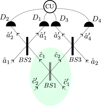
Figure 1: The experimental scheme. Two modes ($\hat{c}^{\prime}_{1}$ and $\hat{c}^{\prime}_{2}$) of a pure twin beam are mixed on beam splitter BS1 to provide a reference two-mode field ($\hat{c}_{1}$ and $\hat{c}_{2}$). The output modes $\hat{c}_{1}$ and $\hat{c}_{2}$ of beam splitter BS1 are combined with two modes $\hat{a}_{1}$ and $\hat{a}_{2}$ of an unknown two-mode Gaussian state at balanced beam splitters BS2 and BS3. The photocount statistics of four output modes $\hat{a}^{\prime}_{j}$, $j=1,\ldots,4$, leaving beam splitters BS2 and BS3 are measured by detectors $D_{1}$, $D_{2}$, $D_{3}$, $D_{4}$ and correlation unit CU.

It relies on mixing the analyzed state with a reference twin beam. However, a pure twin beam composed of only photon pairs and exhibiting the thermal photon-number statistics in the signal and idler fields is not sufficient for this task that requires all the coefficients of the reference covariance matrix being nonzero. For this reason, we first mix the signal (annihilation operator $\hat{c}^{\prime}_{1}$) and idler ($\hat{c}^{\prime}_{2}$) fields on a beam splitter BS1 with the varying transmissivity $t_{1}$. At the output ports of beam splitter BS1 and depending on the transmissivity $t_{1}$, there occur different kinds of states useful in the reconstruction [20, 25]. In the proposed method, the reference light at the output ports ($\hat{c}_{1}$ and $\hat{c}_{2}$) of beams splitter BS1 is superimposed with the analyzed two-mode Gaussian state at balanced beam splitters BS2 and BS3. The output ports ($\hat{a^{\prime}}_{j}$, $j=1,\ldots,4$) of beam splitters BS2 and BS3 are then monitored by four detectors measured in coincidence.

The unitary transformations describing the functioning of three beam splitters BS_j with amplitude transmissivities $t_{j}$ and phase shifts $\theta_{j}$, $j=1,2,3$, are expressed in general as follows:

$$\begin{pmatrix}\hat{c}_{1}\\ \hat{c}_{2}\end{pmatrix} = \begin{pmatrix}t_{1}&r_{1}\exp(i\theta_{1})\\ -r_{1}\exp(-i\theta_{1})&t_{1}\end{pmatrix}\begin{pmatrix}\hat{c}^{\prime}_{1}\\ \hat{c}^{\prime}_{2}\end{pmatrix},$$

$$\begin{pmatrix}\hat{a}^{\prime}_{1}\\ \hat{a}^{\prime}_{2}\end{pmatrix} = \begin{pmatrix}t_{2}&r_{2}\exp(i\theta_{2})\\ -r_{2}\exp(-i\theta_{2})&t_{2}\end{pmatrix}\begin{pmatrix}\hat{a}_{1}\\ \hat{c}_{1}\end{pmatrix},$$

$$\begin{pmatrix}\hat{a}^{\prime}_{3}\\ \hat{a}^{\prime}_{4}\end{pmatrix} = \begin{pmatrix}t_{3}&r_{2}\exp(i\theta_{3})\\ -r_{3}\exp(-i\theta_{3})&t_{3}\end{pmatrix}\begin{pmatrix}\hat{a}_{2}\\ \hat{c}_{2}\end{pmatrix},$$ (13)

where the annihilation operators $\hat{a}_{1}$ and $\hat{a}_{2}$ belong to the modes of the analyzed two-mode Gaussian state.

Assuming the balanced beam splitters BS2 and BS3 ($t_{2}=t_{3}=1/\sqrt{2}$) with zero phase shifts ($\theta_{2}=\theta_{3}=0$) and applying the relations in Eqs. (4), we reveal the following formulas giving the number operators $\hat{n}^{\prime}_{j}$ of fields at the detectors as functions of the operators of the analyzed state and the reference state:

$$\hat{n}^{\prime}_{1} = \hat{a^{\prime}}_{1}^{\dagger}\hat{a}^{\prime}_{1}=\frac{1}{2}\left(\hat{a}_{1}^{\dagger}\hat{a}_{1}+\hat{a}_{1}^{\dagger}\hat{c}_{1}+\hat{a}_{1}\hat{c}_{1}^{\dagger}+\hat{c}_{1}^{\dagger}\hat{c}_{1}\right),$$

$$\hat{n}^{\prime}_{2} = \hat{a^{\prime}}_{2}^{\dagger}\hat{a}^{\prime}_{2}=\frac{1}{2}\left(\hat{a}_{1}^{\dagger}\hat{a}_{1}-\hat{a}_{1}^{\dagger}\hat{c}_{1}-\hat{a}_{1}\hat{c}_{1}^{\dagger}+\hat{c}_{1}^{\dagger}\hat{c}_{1}\right),$$

$$\hat{n}^{\prime}_{3} = \hat{a^{\prime}}_{3}^{\dagger}\hat{a}^{\prime}_{3}=\frac{1}{2}\left(\hat{a}_{2}^{\dagger}\hat{a}_{2}+\hat{a}_{2}^{\dagger}\hat{c}_{2}+\hat{a}_{2}\hat{c}_{2}^{\dagger}+\hat{c}_{2}^{\dagger}\hat{c}_{2}\right),$$

$$\hat{n}^{\prime}_{4} = \hat{a^{\prime}}_{4}^{\dagger}\hat{a}^{\prime}_{4}=\frac{1}{2}\left(\hat{a}_{2}^{\dagger}\hat{a}_{2}-\hat{a}_{2}^{\dagger}\hat{c}_{2}-\hat{a}_{2}\hat{c}_{2}^{\dagger}+\hat{c}_{2}^{\dagger}\hat{c}_{2}\right).$$ (14)

The normally-ordered characteristic function $C_{\cal N}$ of the four-mode Gaussian state characterizing the four fields in front of detectors is written as

$$C_{\cal N}(\beta_{1},\beta_{2},\beta_{3},\beta_{4})=\mathrm{Tr}\left[\hat{\rho}^{\prime}(0)\exp\left(\sum\limits_{i=1}^{4}\beta_{i}\hat{a^{\prime}}^{\dagger}_{i}\right)\exp\left(-\sum\limits_{i=1}^{4}\beta^{\ast}_{i}\hat{a}^{\prime}_{i}\right)\right].$$ (15)

The quantum-mechanical averaging in Eq. (15) is performed by the statistical operator $\hat{\rho}^{\prime}(0)=\hat{\rho}_{12}(0)\otimes\hat{\rho}^{R}(0)$, where $\hat{\rho}_{12}$ is the statistical operator of the unknown two-mode Gaussian state and the operator $\hat{\rho}^{R}$ describes the incident reference twin beam.

Given Eqs. (2) and (15), the normally-ordered characteristic function $C_{\cal N}$ is obtained in the form:

$$C_{\cal N}(\beta_{1},\beta_{2},\beta_{3},\beta_{4})=$$

$$\exp\left\{-\sum\limits_{i=1}^{4}B^{\prime}_{i}|\beta_{i}|^{2}+\left[\frac{1}{2}\sum\limits_{i=1}^{4}C^{\prime}_{i}\beta_{i}^{\ast 2}+\sum\limits_{j<k}^{4}D^{\prime}_{jk}\beta_{j}^{\ast}\beta_{k}^{\ast}+\sum\limits_{j<k}^{4}\bar{D}^{\prime}_{jk}\beta_{j}\beta_{k}^{\ast}+{\rm c.c.}\right]\right\},$$

where the coefficients $B^{\prime}_{i}$, $C^{\prime}_{i}$, $D^{\prime}_{jk}$, and $\bar{D}^{\prime}_{jk}$ are determined by the formulas written in Eqs. (2).

Denoting the normally-ordered photon-number moments $\langle\hat{n}^{k}\rangle_{\cal N}$ as moments $\langle W^{k}\rangle_{\cal N}$ of the integrated intensities, as suggested by the photodetection theory [17], we derive the second-order correlations of the integrated-intensity fluctuations $\Delta W$ in different modes from Eq. (4) in the form:

$$\langle\Delta W_{j}\Delta W_{k}\rangle_{\cal N}=\langle\hat{a^{\prime}}_{j}^{\dagger}\hat{a^{\prime}}_{k}^{\dagger}\hat{a}^{\prime}_{j}\hat{a}^{\prime}_{k}\rangle-\langle\hat{a^{\prime}}_{j}^{\dagger}\hat{a}^{\prime}_{j}\rangle\langle\hat{a^{\prime}}_{k}^{\dagger}\hat{a}^{\prime}_{k}\rangle$$

$$=\left.\frac{\partial^{4}C_{\cal N}}{\partial\beta_{j}\partial(-\beta_{j}^{*})\partial\beta_{k}\partial(-\beta_{k}^{*})}\right|_{\{\beta_{j}\}=\{\beta_{j}^{*}\}=0}-\left.\frac{\partial^{2}C_{\cal N}}{\partial\beta_{j}\partial(-\beta_{j}^{*})}\frac{\partial^{2}C_{\cal N}}{\partial\beta_{k}\partial(-\beta_{k}^{*})}\right|_{\{\beta_{j}\}=\{\beta_{j}^{*}\}=0}$$

$$=|D^{\prime}_{jk}|^{2}+|\bar{D}^{\prime}_{jk}|^{2},\hskip 14.22636ptj\neq k.$$ (17)

Now, applying the photodetection theory for the detectors with quantum detection efficiencies $\eta_{j}$ and dark-count rates $n_{dj}$, we arrive at the following second-order moments of photocount fluctuations at all four detectors:

$$\langle\Delta\hat{m}_{j}\Delta\hat{m}_{k}\rangle=\eta_{j}\eta_{k}\langle\Delta W_{j}\Delta W_{k}\rangle_{\cal N},\quad j\neq k.$$ (18)

Applying further Eqs. (2), (4) and (4), we reveal the following second-order moments of photocount fluctuations:

$$\langle\Delta\hat{m}_{1}\Delta\hat{m}_{2}\rangle = \frac{\eta_{1}\eta_{2}}{4}\Big{(}B_{1}^{2}+|C_{1}|^{2}+B_{1}^{R2}+|C_{1}^{R}|^{2}-2B_{1}B_{1}^{R}-2{\rm Re}\{C_{1}C_{1}^{R\ast}\}\Big{)},$$

$$\langle\Delta\hat{m}_{3}\Delta\hat{m}_{4}\rangle = \frac{\eta_{3}\eta_{4}}{4}\Big{(}B_{2}^{2}+|C_{2}|^{2}+B_{2}^{R2}+|C_{2}^{R}|^{2}-2B_{2}B_{2}^{R}-2{\rm Re}\{C_{2}C_{2}^{R\ast}\}\Big{)},$$

$$\langle\Delta\hat{m}_{1}\Delta\hat{m}_{3}\rangle = \frac{\eta_{1}\eta_{3}}{4}\Big{(}|D_{12}|^{2}+|\bar{D}_{12}|^{2}+|D_{12}^{R}|^{2}+|\bar{D}_{12}^{R}|^{2}+2{\rm Re}\{D_{12}D_{12}^{R\ast}\}+$$

$$2{\rm Re}\{\bar{D}_{12}\bar{D}_{12}^{R\ast}\}\Big{)},$$

$$\langle\Delta\hat{m}_{1}\Delta\hat{m}_{4}\rangle = \frac{\eta_{1}\eta_{4}}{4}\Big{(}|D_{12}|^{2}+|\bar{D}_{12}|^{2}+|D_{12}^{R}|^{2}+|\bar{D}_{12}^{R}|^{2}-2{\rm Re}\{D_{12}D_{12}^{R\ast}\}-$$

$$2{\rm Re}\{\bar{D}_{12}\bar{D}_{12}^{R\ast}\}\Big{)},$$

$$\langle\Delta\hat{m}_{2}\Delta\hat{m}_{3}\rangle = \frac{\eta_{2}\eta_{3}}{4}\Big{(}|D_{12}|^{2}+|\bar{D}_{12}|^{2}+|D_{12}^{R}|^{2}+|\bar{D}_{12}^{R}|^{2}-2{\rm Re}\{D_{12}D_{12}^{R\ast}\}-$$

$$2{\rm Re}\{\bar{D}_{12}\bar{D}_{12}^{R\ast}\}\Big{)},$$

$$\langle\Delta\hat{m}_{2}\Delta\hat{m}_{4}\rangle = \frac{\eta_{2}\eta_{4}}{4}\Big{(}|D_{12}|^{2}+|\bar{D}_{12}|^{2}+|D_{12}^{R}|^{2}+|\bar{D}_{12}^{R}|^{2}+2{\rm Re}\{D_{12}D_{12}^{R\ast}\}+$$ (19)

$$2{\rm Re}\{\bar{D}_{12}\bar{D}_{12}^{R\ast}\}\Big{)}.$$

The formulas in Eqs. (4), when applied to the analyzed two-mode Gaussian state and the reference twin beam, allow to recover all coefficients of the covariance matrix of the analyzed state. The determination of the coefficients is naturally split into the following four steps.

Retrieving the coefficients $B_{1}$ and $B_{2}$ — These coefficients give the mean numbers of photons present in both modes of the analyzed state. If the inputs of the reference field are replaced by the vacuum, we immediately arrive at the values of these coefficients using the relations in Eqs. (4):

$$B_{1}=2\left(\langle\hat{m}_{1}\rangle-n_{d1}\right)/\eta_{1}, B_{2}=2\left(\langle\hat{m}_{3}\rangle-n_{d3}\right)/\eta_{3}.$$ (20)

Retrieving the coefficients $C_{1}$ and $C_{2}$ — To reveal these coefficients, we exploit the fact that a pure twin beam with the mean photon-pair number $B_{p}$ gives two separable squeezed states with opposite phases $\phi$ when its constituents are combined at the balanced beam splitter BS1 [28]. Thus, the reference field attains the coefficients $B_{1}^{R}=B_{2}^{R}=B_{\rm p}$, $C_{1}^{R}=-C_{2}^{R}=i\exp(i\phi)\sqrt{B_{\rm p}(B_{\rm p}+1)}$ [25] and the suitable relations in Eqs. (4) can be recast into the form:

$$\langle\Delta\hat{m}_{1}\Delta\hat{m}_{2}\rangle = \frac{\eta_{1}\eta_{2}}{4}\Big{(}2B_{\rm p}^{2}+B_{\rm p}(1-2B_{1})+\langle\Delta W_{1}^{2}\rangle_{\cal N}\Big{)}-$$

$$\frac{\eta_{1}\eta_{2}\sqrt{B_{\rm p}(B_{\rm p}+1)}}{2}{\rm Im}\left\{\exp\left(-i\phi\right)C_{1}\right\},$$

$$\langle\Delta\hat{m}_{3}\Delta\hat{m}_{4}\rangle = \frac{\eta_{3}\eta_{4}}{4}\Big{(}2B_{\rm p}^{2}+B_{\rm p}(1-2B_{2})+\langle\Delta W_{2}^{2}\rangle_{\cal N}\Big{)}+$$ (21)

$$\frac{\eta_{3}\eta_{4}\sqrt{B_{\rm p}(B_{\rm p}+1)}}{2}{\rm Im}\left\{\exp\left(-i\phi\right)C_{2}\right\}.$$

The formulas in Eq. (21) allow us to determine the variances $\langle\Delta W_{j}^{2}\rangle_{\cal N}$ for $j=1,2$ of the constituents of the analyzed field provided that the reference field is absent. The usual formula for the second moment $\langle W_{j}^{2}\rangle_{\cal N}$ of integrated intensity of mode $j$, $\langle W_{j}^{2}\rangle_{\cal N}=2B_{j}^{2}+|C_{j}|^{2}$, can be recast into that for the variance $\langle\Delta W_{j}^{2}\rangle_{\cal N}=B_{j}^{2}+|C_{j}|^{2}$, that immediately provides the absolute value $|C_{j}|$. For the complex coefficients $C_{j}$, we need to vary the phase $\phi$ of the reference field, that is derived from the pump field that created the reference pure twin beam. The obtained interference pattern then gives us both the magnitudes and phases of both coefficients.

If the analyzed state is known to be symmetric ($B_{1}=B_{2}$ and $C_{1}=C_{2}\equiv C$), we can even apply the following simpler formula to arrive at the coefficient $C$:

$$\frac{1}{\sqrt{B_{\rm p}(B_{\rm p}+1)}}\left(\frac{\langle\Delta\hat{m}_{3}\Delta\hat{m}_{4}\rangle}{\eta_{3}\eta_{4}}-\frac{\langle\Delta\hat{m}_{1}\Delta\hat{m}_{2}\rangle}{\eta_{1}\eta_{2}}\right)={\rm Im}\left\{\exp\left(-i\phi\right)C\right\}.$$ (22)

Retrieving the coefficient $D_{12}$ — We need as a reference field the original pure twin beam for which $D_{12}^{R}$ is given in Eq. (12) and $\bar{D}_{12}^{R}$ vanishes. The third and fourth relations in Eqs. (4) can be rearranged into the formula:

$$\frac{1}{\sqrt{B_{\rm p}(B_{\rm p}+1)}}\left(\frac{\langle\Delta\hat{m}_{1}\Delta\hat{m}_{3}\rangle}{\eta_{1}\eta_{3}}-\frac{\langle\Delta\hat{m}_{1}\Delta\hat{m}_{4}\rangle}{\eta_{1}\eta_{4}}\right)={\rm Im}\left\{\exp\left(-i\phi\right)D_{12}\right\}.$$ (23)

According to Eq. (23), the variation of the pump phase $\phi$ provided both the magnitude and phase of coefficient $D_{12}$. We note that also other combinations of the second-order moments in Eqs. (4) can be used to reveal the coefficient $D_{12}$.

Retrieving the coefficient $\bar{D}_{12}$ — To retrieve the coefficient $\bar{D}_{12}$ one needs a nonzero coefficient $\bar{D}_{12}^{R}$ of the reference field. Such coefficient cannot be obtained by a simple mixing of the constituents of a pure twin beam on beam splitter BS1. However, if we consider only one constituent of the pure twin beam and mix it with the vacuum state of beam splitter BS1 with transmissivity $t_{1}=1/\sqrt{2}$, we arrive at the fields with zero values $D_{12}^{R}$, $C_{1}^{R}$ and $C_{2}^{R}$, but nonzero coefficients $B_{1}^{R}=B_{2}^{R}=B_{\rm p}/2$ and $\bar{D}_{12}^{R}=\pm B_{\rm p}/2$, where the plus (minus) sign is taken for mode $\hat{c}^{\prime}_{2}$ ($\hat{c}^{\prime}_{1}$) in the vacuum state. In this case, the following relation is revealed:

$$\frac{\langle\Delta\hat{m}_{1}\Delta\hat{m}_{3}\rangle}{\eta_{1}\eta_{3}}-\frac{\langle\Delta\hat{m}_{1}\Delta\hat{m}_{4}\rangle}{\eta_{1}\eta_{4}}={\rm Re}\{\bar{D}_{12}^{R}\bar{D}_{12}^{*}\}.$$ (24)

The formula in Eq. (24) suggests that the variation of complex phase of the reference coefficient $\bar{D}_{12}^{R}$ allows to recover the coefficient $\bar{D}_{12}$ of the analyzed field. This can easily be accomplished by imposing a variable phase shift $\theta$ to, e.g., mode $\hat{c}_{1}$ by a phase modulator placed between the beam splitters BS1 and BS2 [$\hat{c}_{1}\rightarrow\exp(i\theta)\hat{c}_{1}$]. In this case, Eq. (24) is transformed into the form

$$\frac{2}{B_{\rm p}}\left(\frac{\langle\Delta\hat{m}_{1}\Delta\hat{m}_{3}\rangle}{\eta_{1}\eta_{3}}-\frac{\langle\Delta\hat{m}_{1}\Delta\hat{m}_{4}\rangle}{\eta_{1}\eta_{4}}\right)=\pm{\rm Re}\{\exp(-i\theta)\bar{D}_{12}^{*}\},$$ (25)

where again the plus (minus) sign is taken for the mode $\hat{c}^{\prime}_{2}$ ($\hat{c}^{\prime}_{1}$) in the vacuum state. According to Eq. (25) the variation of phase $\theta$ then provides both the real and imaginary part of the coefficient $\bar{D}_{12}$.

In the experiment, a source of identical reference pure twin beams is needed. If we consider such two beams in the analyzed scheme, one as a reference beam and the other as a beam in an unknown state, the parameters of the reference twin beam can be reached. This allows to check the quality of the applied reference twin beam, that is assumed to be ideally composed only of photon pairs.

At the end, we note that the developed method can be generalized to allow for the characterization of two-mode Gaussian states with nonzero coherent components. In this case, the coherent components in both modes of the analyzed state have to be identified first, by applying the homodyne detection scheme. Then, the above written formulas can be generalized to include the coherent components. So the contributions from coherent components can easily be subtracted.

5 Conclusions

We have suggested a method for characterizing a general two-mode Gaussian state with vanishing coherent components. The coefficients of its normally-ordered covariance matrix are revealed by mixing the analyzed state with a reference beam obtained from a pure twin beam, by using two balanced beam splitters. The variation of the phase of the pump beam that generates the reference twin beam together with the variation of the phase of one mode of the reference beam are needed in the method that monitors the first- and second-order moments of photocounts at four detectors placed in the experimental setup.

References

References

• Agarwal [2013] G. Agarwal, Quantum Optics, Cambridge University Press, Cambridge, UK, 2013.
• Helstrom [1976] C. W. Helstrom, Quantum Detection and Estimation Theory, Academic Press, New York, 1976.
• Glauber [2007] R. J. Glauber, Quantum Theory of Optical Coherence: Selected Papers and Lectures, Wiley-VCH, Weinheim, 2007.
• Raymer et al. [1994] M. G. Raymer, M. Beck, D. McAlister, Complex wave-field reconstruction using phase-space tomography, Phys. Rev. Lett. 72 (1994) 1137–1140.
• Bouwmeester et al. [1997] D. Bouwmeester, J. W. Pan, K. Mattle, M. Eibl, H. Weinfurter, A. Zeilinger, Experimental quantum teleportation, Nature 390 (1997) 575–579.
• Braunstein and Kimble [2000] S. L. Braunstein, H. J. Kimble, Dense coding for continuous variables, Phys. Rev. A 61 (2000) 042302.
• Bruß et al. [2004] D. Bruß, G. M. D’Ariano, M. Lewenstein, C. Macchiavello, A. Sen(De), U. Sen, Distributed quantum dense coding, Phys. Rev. Lett. 93 (2004) 210501.
• Jennewein et al. [2000] T. Jennewein, C. Simon, G. Weihs, H. Weinfurter, A. Zeilinger, Quantum cryptography with entangled photons, Phys. Rev. Lett. 84 (2000) 4729–4732.
• Gisin et al. [2011] N. Gisin, G. Ribordy, W. Tittel, H. Zbinden, Quantum cryptography, Rev. Mod. Phys. 74 (2011) 145—195.
• Lvovsky and Raymer [2009] A. I. Lvovsky, M. G. Raymer, Continuous-variable optical quantum-state tomography, Rev. Mod. Phys. 81 (2009) 299–332.
• Shchukin et al. [2005] E. Shchukin, T. Richter, W. Vogel, Nonclassicality criteria in terms of moments, Phys. Rev. A 71 (2005) 011802(R).
• Miranowicz et al. [2010] A. Miranowicz, M. Bartkowiak, X. Wang, Y. X. Liu, F. Nori, Testing nonclassicality in multimode fields: A unified derivation of classical inequalities, Phys. Rev. A 82 (2010) 013824.
• Banaszek and Wódkiewicz [1996] K. Banaszek, K. Wódkiewicz, Direct probing of quantum phase space by photon counting, Phys. Rev. Lett. 76 (1996) 4344–4347.
• Zambra et al. [2005] G. Zambra, A. Andreoni, M. Bondani, M. Gramegna, M. Genovese, G. Brida, A. Rossi, M. G. A. Paris, Experimental reconstruction of photon statistics without photon counting, Phys. Rev. Lett. 95 (2005) 063602.
• Bondani et al. [2009] M. Bondani, A. Allevi, A. Andreoni, Wigner function of pulsed fields by direct detection, Opt. Lett. 34 (2009) 1444–1446.
• Harder et al. [2014] G. Harder, D. Mogilevtsev, N. Korolkova, C. Silberhorn, Tomography by noise, Phys. Rev. Lett. 113 (2014) 070403.
• Peřina [1991] J. Peřina, Quantum Statistics of Linear and Nonlinear Optical Phenomena, Kluwer, Dordrecht, 1991.
• Haderka et al. [2005] O. Haderka, J. Peřina Jr., M. Hamar, J. Peřina, Direct measurement and reconstruction of nonclassical features of twin beams generated in spontaneous parametric down-conversion, Phys. Rev. A 71 (2005) 033815.
• Peřina Jr. et al. [2012] J. Peřina Jr., M. Hamar, V. Michálek, O. Haderka, Photon-number distributions of twin beams generated in spontaneous parametric down-conversion and measured by an intensified ccd camera, Phys. Rev. A 85 (2012) 023816.
• Arkhipov et al. [2016] I. I. Arkhipov, J. J. Peřina, J. Svozilík, A. Miranowicz, Nonclassicality invariant of general two-mode Gaussian states, arXiv:1601.04868 (2016).
• Peřina Jr. et al. [2013] J. Peřina Jr., O. Haderka, V. Michálek, M. Hamar, State reconstruction of a multimode twin beam using photodetection, Phys. Rev. A 87 (2013) 022108.
• van Loock and Furusawa [2003] P. van Loock, A. Furusawa, Detecting genuine multipartite continuous-variable entanglement, Phys. Rev. A 67 (2003) 052315.
• Adesso et al. [2006] G. Adesso, A. Serafini, F. Illuminati, Multipartite entanglement in three-mode gaussian states of continuous-variable systems: Quantification, sharing structure, and decoherence, Phys. Rev. A 73 (2006) 032345.
• Altepeter et al. [2003] J. B. Altepeter, D. Branning, E. Jeffrey, T. C. Wei, P. G. Kwiat, R. T. Thew, J. L. O’Brien, M. A. Nielsen, A. G. White, Ancilla-assisted quantum process tomography, Phys. Rev. Lett. 90 (2003) 193601.
• Arkhipov et al. [2016] I. I. Arkhipov, J. J. Peřina, J. Peřina, A. Miranowicz, The interplay of nonclassicality and entanglement of Gaussian fields in optical parametric processes, (submitted to PRA) (2016).
• Peřina and Křepelka [2011] J. Peřina, J. Křepelka, Joint probability distribution and entanglement in optical parametric processes, Opt. Commun. 284 (2011) 4941–4950.
• Allevi et al. [2013] A. Allevi, M. Lamperti, M. Bondani, J. Peřina Jr., V. Michálek, O. Haderka, R. Machulka, Characterizing the nonclassicality of mesoscopic optical twin-beam states, Phys. Rev. A 88 (2013) 063807.
• Paris [1997] M. G. A. Paris, Joint generation of identical squeezed states, Phys. Lett. A 225 (1997) 28.