Adaptive Combination of -LMS Adaptive Filters for Sparse System Identification in Fluctuating Noise Power
Abstract
Recently, the -least mean square (-LMS) algorithm has been proposed to identify sparse linear systems by employing a sparsity-promoting continuous function as an approximation of pseudonorm penalty. However, the performance of this algorithm is sensitive to the appropriate choice of the some parameter responsible for the zero-attracting intensity. The optimum choice for this parameter depends on the signal-to-noise ratio (SNR) prevailing in the system. Thus, it becomes difficult to fix a suitable value for this parameter, particularly in a situation where SNR fluctuates over time. In this work, we propose several adaptive combinations of differently parameterized -LMS to get an overall satisfactory performance independent of the SNR, and discuss some issues relevant to these combination structures. We also demonstrate an efficient partial update scheme which not only reduces the number of computations per iteration, but also achieves some interesting performance gain compared with the full update case. Then, we propose a new recursive least squares (RLS)-type rule to update the combining parameter more efficiently. Finally, we extend the combination of two filters to a combination of number adaptive filters, which manifests further improvement for .
1 Introduction
Exploiting sparsity of the identifiable system has been a celebrated topic in the last decade among adaptive filtering research community. However, it has a long and diverse history within and outside the adaptive signal processing community. Researchers in the field of of network and acoustic echo cancellation have tried to take advantage of the sparse echo path models for improving the performance of the echo cancellation algorithms. Adaptive sparse system identification has also found applications in the field of sparse wireless multipath channel estimation and shallow underwater acoustic communication channel estimation. Starting from the adaptive delay filters and active tap detection based algorithms to the popular family of proportionate-type adaptive filters and recently proposed set theoretic adaptive filters, numerous attempts have been made to use the a priori knowledge about system sparsity.
Another family of sparsity-promoting norm regularized algorithms has gained immense popularity in recent years. Historically, the basis pursuit and other related methods have shown advantages of this approach. After the advent of sparse signal reconstruction techniques in the compressive sensing literatures, different sparsity-promoting norms have been borrowed by the adaptive filtering researchers.
Though the -pseudonorm which measures the sparsity by counting the number of nonzero elements in a vector can not be directly used for the regularization purpose since it is not a continuous function. Several approximations of this have been considered. The -norm or the absolute sum, the log-sum have been studied to a reasonable extent in this context, and have given birth to the algorithms like ZA-LMS and the RZA-LMS. Another approximation of -norm by some exponential function has also been proposed. This algorithm manifests excellent behaviour in terms of convergence speed and steady-state mean square deviation for proper choice of a parameter responsible for zero-attracting intensity.
In section , we provide a brief review of the algorithm.
In section , it has been shown that the choice of this parameter is sensitive to the signal-to-noise ratio (SNR) of the setup. An adaptive technique has been proposed to tackle this problem but with increasing complexity of the algorithm.
In section , we propose a convex combination of two differently parameterized -LMS adaptive filters to alleviate the sensitivity of selection of this parameter to some extent. We also demonstrate the simulation results to support the advantage of the proposed scheme.
In section , we discuss a reduced-complexity partial update scheme for this combination. In this section, we also derive a new recursive least squares (RLS) type update rule for efficient adaptation of the combining parameter. The simulation results, we provide in this section, show how this update scheme proves to be a better alternative of the conventional gradient descent based update rule.
In section , we extend the techniques presented in the earlier sections to a more general combination of number of adaptive filters.
2 Brief Review of the -LMS Algorithm
For deriving the -LMS algorithm, the cost function is modified as
| (1) |
Considering that the -norm minimization is a Non-Polynomial (NP) hard problem, -norm is generally approximated by a continuous function. A popular approximation is
| (2) |
By minimizing the above cost function the gradient descent recursion for the filter coefficient becomes
| (3) |
To reduce the computational complexity, the first order Taylor series expansion of exponential functions is taken into consideration,
| (4) | |||||
It is to be noted that the above approximation is bounded to be positive because the exponential function is larger than zero.
Now, the approximated gradient descent recursion is
| (5) |
where
3 The Dependence of the Optimum on the Signal-to-Noise Ratio (SNR)
In this section, we try to show how the optimum depends on the signal-to-noise ratio (SNR).
.
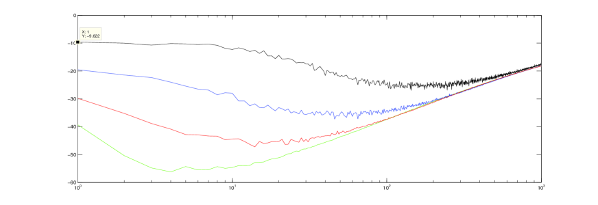
Experiment : We try to identify a sparse FIR system of length , which has only five nonzero coefficients (set as ), and rest of them are zeros. We use a zero mean, unit variance white Gaussian random process as input to the unknown system as well as the -LMS adaptive filter. The parameters of the algorithm are set as: , . Matlab simulations are run for samples and steady-state MSD is calculated by averaging repeating the experiment over iterations. The value of is varied from to with steps, and the steady-state MSD is plotted against in Fig.. Four different noise variances are chosen for the experiment. The black, blue, red and green curves correspond to dB, dB, dB, dB SNR-s respectively.
The optimum for which the minimum MSD is achieved is different for different SNRs. It explicitly implies that when SNR is likely to fluctuate over a wide range, a fixed single can not guarantee the best result for all different cases. This fact motivates us to propose a convex combination of two -LMS adaptive filters with two different values.
4 Proposed Adaptive Convex Combination of Two Differently Parameterized -LMS Adaptive Filters
In this section, we propose a convex combination of two -LMS adaptive filters. In this part of the paper, we have constrained ourselves to use the convex combination scheme in []. The outputs of the two -LMS adaptive filters are combined using the following rule:
| (6) |
where is the output of the adaptive filter (), and is the combined output.
These two filters are identical in all aspects apart from their individual values of .
| (7) |
The update rule for the parameter is as follows:
| (8) |
where .
It is also noteworthy that is constrained within the range of . This is a common practice to avoid being stucked at any of the two extremes of its unconstrained range.
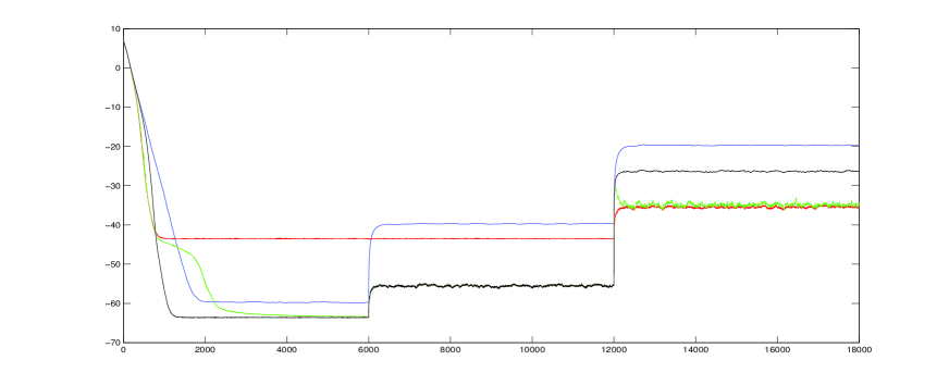
Experiment : The values are chosen as and . Three SNR values are chosen as dB, dB and dB. The simulation starts with dB SNR, at the iteration noise power increases to give a SNR of dB, and finally, it becomes dB at the iteration. The simulation stops at the iteration. The MSD-s are obtained by averaging independent runs of this simulation. The is kept at . All other parameters and variables are same as in the experiment . The instantaneous MSD-s are plotted against iteration index in fig.2. The proposed combination (plotted in green) achieves the best steady-state MSDs for all SNR levels. The red and the black curves represent two -LMS filters (for and respectively.)
.
5 A Reduced Complexity Partial Update Scheme
One of the major drawbacks of the combination schemes, in general, is the increase in the number of computations per iteration by a multiple factor for deployment of multiple adaptive filters simultaneously. In this section, we demonstrate a partial update scheme for reducing the computational burden. We divide the set of all filter taps into two mutually exclusive subsets, named as and for all odd and all even taps respectively. We update the filter taps of these individual subsets at alternative iterations. Now, one natural question that can arise is how we choose the subsets for individual component filters. Is it same for all the filters? Or, it is rather more beneficial to choose different subsets for different filters at a particular iteration. For the time being, we go for the second option without discussing the relative merits and demerits of this choice. We leave this discussion for the section .
Initialization : for each adaptive filter . number of diagonal matrices defined as , for which for , and otherwise. For every index and every adaptive filter , repeat (9)
5.1 A New RLS-type Update Rule for Adapting the Combining Parameter
We also derive a new update rule for in the following. Let us first define the least-squares cost function as
| (10) |
where is the error at the instant for the combined filter.
can be expanded by
| (11) |
The optimum value of , can be found as
| (12) | |||||
where
, and .
Now,defining , , , we get
| (14) |
Now, to derive a recursive update for using and , we write
| (15) | |||||
where
| (16) |
But, since this update does not constrain within and , we update the corresponding variable , and then compute using the aforementioned rule. Since is a monotonically increasing function , the same incremental update has been used for as above.
| (17) |
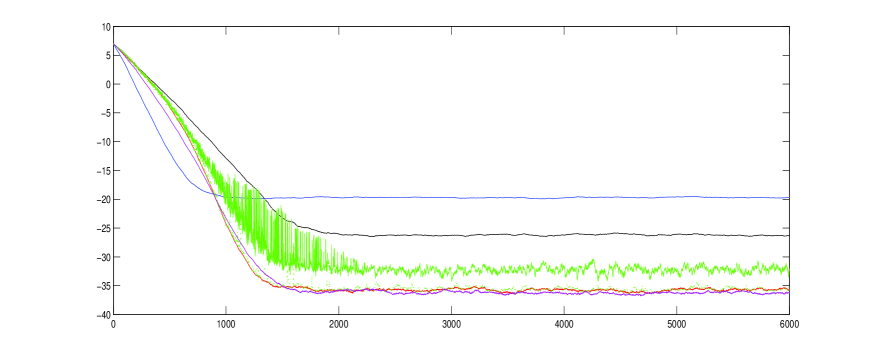
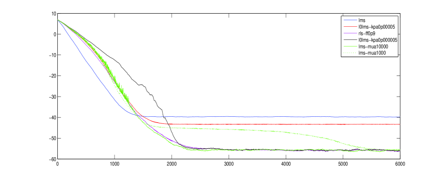
Experiment : Now, we repeat the experiment with both the conventional gradient descent based update and the propose RLS-type update for the combiner separately, and we also incorporate the aforementioned partial update with mutually exclusive subsets scheme mentioned in the table I for case. We plot both the MSDs as well as the individual MSDs for the component filters and the simple LMS adaptive filter in fig.4 and fig.5 for SNR dB and dB respectively. For gradient descent based update, we plot two different curves for two different values of , i.e., and . For a particular SNR, one proves to be better than other. But, the RLS-type update shows its superiority by providing satisfactory behaviour in both situations without tuning its forgetting factor.
.
.
6 An Adaptive Convex Combination of Number of Filters
In this section, we extend our work to a more general case of combining adaptive filters so that a much wider range of SNR can be covered. We also modify the RLS-type combiner update rule for this general case. The derivation is skipped here. The rule is shown in the Table .
Initialization : for each . for and elsewhere. (for to ) For every index and every adaptive filter, repeat
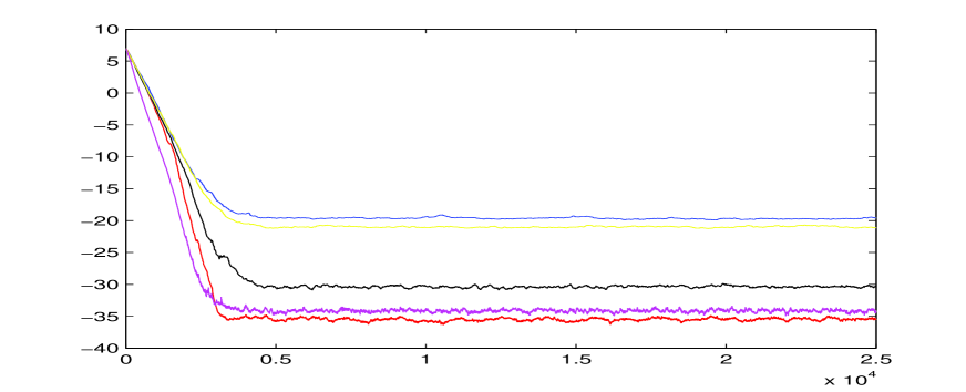
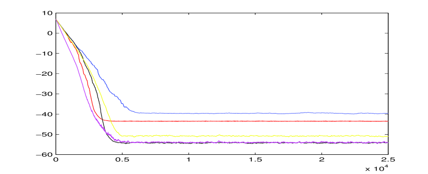
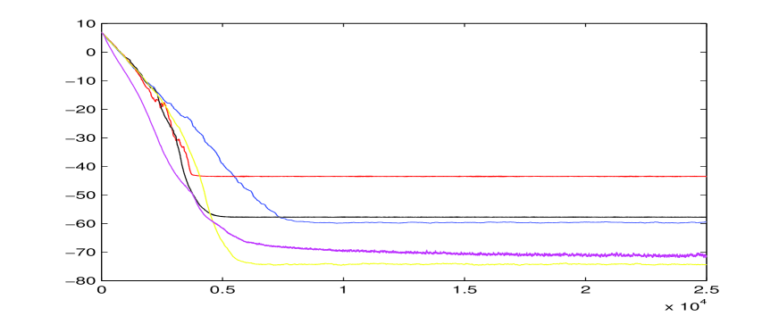
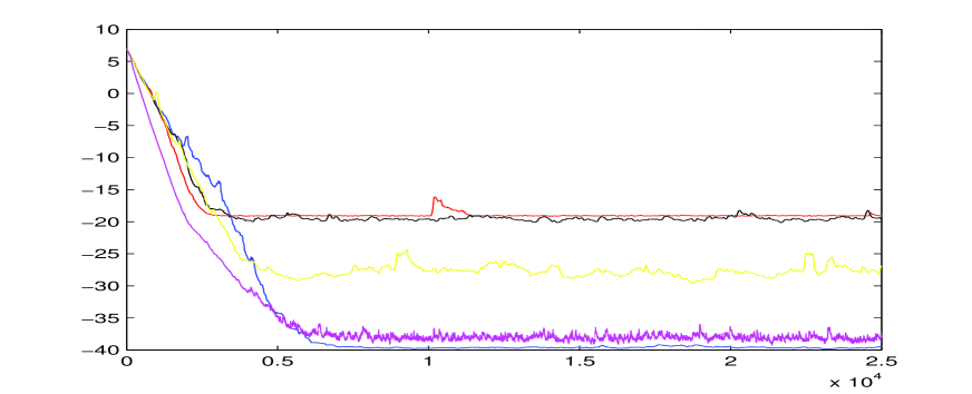
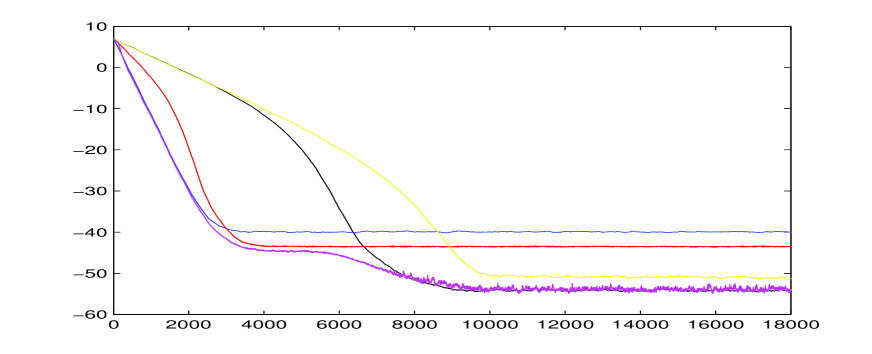
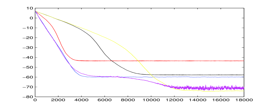
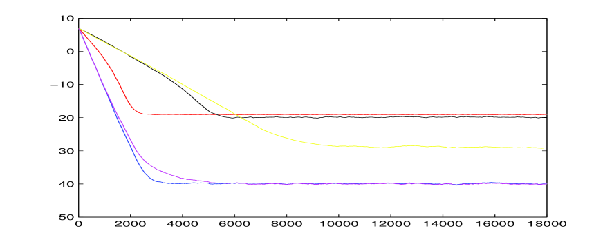
Experiment : We perform four separate experiments with three different SNR levels, i.e. dB, dB, dB and dB (with a different unknown system described below). In each case, the new combined adaptive filter () is deployed to identify the aforementioned sparse unknown FIR system. The parameters of the filters remain same except chosen as , , and . In each case, the robustness of the combination filter (in magenta) can be observed. In fig., a particular case has been studied where the unknown system is chosen as a near-sparse FIR system with all zero coefficients of the unknown system of the earlier experiments are replaced with very small non-zero values.
.
.
.
.
6.1 A Special Advantage of Using Partial Update with Mutually Exclusive Subsets
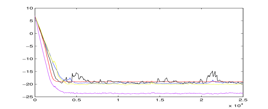
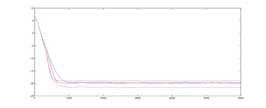
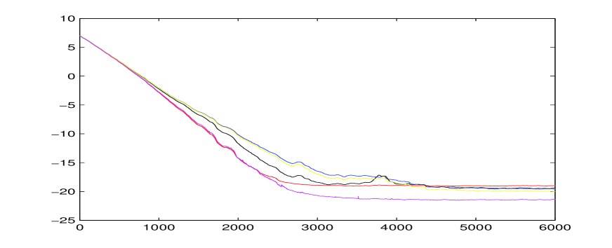
The next three figures demonstrate a special advantage of using the partial update scheme with mutually exclusive subsets compared with full update and PU with non-exclusive subsets. SNR level is dB and the unknown system is the near-sparse one in the last experiment. Here, though none of the component filters shows substantially better than the LMS, the combination manifests excellent performance for the PU with mutually exclusive subsets scheme [Fig.]. Fig. and fig. are respectively for the full update and the PU with same subsets.
.
.
.
7 Partial Update with Uneven Mutually Exclusive Subsets
One major disadvantage of the partial update schemes mentioned in the last section is that it slows down the convergence of the individual adaptive filters as well as the combination by a fraction of . In this section, we describe an uneven division of the filter tap indices into the subsets, and how it helps to alleviate the problem of slow convergence to some extent.
Let us here describe the uneven division of the subsets and how it differs from the one described in the table II. The rule is as follows:
for
and elsewhere.
(for to . is the smallest integer power of greater or equal to )
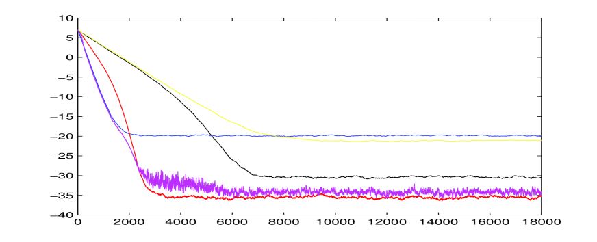
The presence of subsets with larger cardinalities help corresponding individual adaptive filters converge faster than those with smaller subsets. Thus, it leads to a better convergence behaviour for the overall combination as it is seen in the following figures [Fig. 10 -13]. The magenta curve (the combination) always follows the blue one (one with lagest subset) first, then reconverges to the one with lesser steady-state m.s.d.
.
.
.
.
References
- [1] J. Radecki, Z. Zilic, and K. Radecka, “Echo Cancellation in IP Networks”, Proc. Fourty-Fifth Midwest Symposium on Circuits and Systems, vol. 2, 2002, pp. 219-222.
- [2] E. Hansler, “The Hands-free Telephone Problem - an Annotated Bibliography”, Signal Processing, vol. 27, no. 3, pp. 259-271, Jun. 1992.
- [3] W. Schreiber, “Advanced Television Systems for Terrestrial Broadcasting”, Proc. IEEE, vol. 83, no. 6, pp. 958-981, 1995.
- [4] W. Bajwa, J. Haupt, G. Raz and R. Nowak, “Compressed Channel Sensing”, Prof. IEEE CISS, 2008, pp. 5-10.
- [5] M. Kocic, D. Brady and M. Stojanovic, “Sparse Equalization for Real-Time Digital Underwater Acoustic Communications”, Proc. IEEE OCEANS, 1995, pp. 1417-1422.
- [6] D. L. Duttweiler, “Proportionate Normalized Least Mean Square Adaptation in Echo Cancellers”, IEEE Trans. Speech Audio Processing, vol. 8, no. 5, pp. 508-518, Sep., 2000
- [7] J. Benesty, S. L. Gay, “An Improved PNLMS Algorithm”, Proc. IEEE ICASSP, vol. 2, pp. 1881-1884, May 2002, Orlando, Florida, USA.
- [8] H. Deng, and M. Doroslovacki, “Improving Convergence of the PNLMS Algorithm for Sparse Impulse Response Identification”, IEEE Signal Processing Letters, vol. 12, No. 3, pp. 181-184, March 2005.
- [9] R. Baraniuk, “Compressive Sensing”, IEEE Signal Processing Magazine, vol. 25, pp. 21-30, March 2007.
- [10] Y. Gu, Y. Chen and A. O. Hero, “Sparse LMS for System Identification”, Proc. IEEE ICASSP-2009, April 2009, Taipei, Taiwan.
- [11] Y. Gu, J. Jin and S. Mei, ” Norm Constraint LMS Algorithm for Sparse System Identification”, IEEE Signal Processing Letters, vol. 16, No. 9, pp. 774-777, Sept. 2009.
- [12] B. K. Das and M. Chakraborty “Sparse adaptive filtering by an adaptive convex combination of the LMS and the ZA-LMS algorithms,” IEEE Trans. Circuits Syst.I, Reg.Papers, Vol. 61, No. 5, May, 2014.
- [13] Dirk T. M. Slock, “On the Convergence Behavior of the LMS and the Normalized LMS algorithms”, IEEE Trans. on Signal Process., vol. 41, no. 9, pp. 2811-2825, September 1993.
- [14] J. Arenas-García, A. R. Figueiras-Vidal, and A. H. Sayed, “Mean-square performance of a convex combination of two adaptive filters”, IEEE Trans. Signal Proc., vol. 54, no. 3, pp. 1078-1090, March 2006.
- [15] A. Papoulis and S. U. Pillai, Probability, Random Variables and Stochastic Processes (4th edition), New York: McGraw Hill, 2002.
- [16] S. Haykin, Adaptive Filter Theory, Englewood Cliffs, NJ: Prentice-Hall, 1986.