Model’s sparse representation based on reduced mixed GMsFE basis methods

Lijian Jiang Institute of Mathematics, Hunan University, Changsha 410082, China. Email: ljjiang@hnu.edu.cn. Corresponding author    Qiuqi Li College of Mathematics and Econometrics, Hunan University, Changsha 410082, China. Email:qiuqili@hnu.edu.cn.

ABSTRACT

In this paper, we propose a model’s sparse representation based on reduced mixed generalized multiscale finite element (GMsFE) basis methods for elliptic PDEs with random inputs. A typical application for the elliptic PDEs is the flow in heterogeneous random porous media. Mixed generalized multiscale finite element method (GMsFEM) is one of the accurate and efficient approaches to solve the flow problem in a coarse grid and obtain the velocity with local mass conservation. When the inputs of the PDEs are parameterized by the random variables, the GMsFE basis functions usually depend on the random parameters. This leads to a large number degree of freedoms for the mixed GMsFEM and substantially impacts on the computation efficiency. In order to overcome the difficulty, we develop reduced mixed GMsFE basis methods such that the multiscale basis functions are independent of the random parameters and span a low-dimensional space. To this end, a greedy algorithm is used to find a set of optimal samples from a training set scattered in the parameter space. Reduced mixed GMsFE basis functions are constructed based on the optimal samples using two optimal sampling strategies: basis-oriented cross-validation and proper orthogonal decomposition. Although the dimension of the space spanned by the reduced mixed GMsFE basis functions is much smaller than the dimension of the original full order model, the online computation still depends on the number of coarse degree of freedoms. To significantly improve the online computation, we integrate the reduced mixed GMsFE basis methods with sparse tensor approximation and obtain a sparse representation for the model’s outputs. The sparse representation is very efficient for evaluating the model’s outputs for many instances of parameters. To illustrate the efficacy of the proposed methods, we present a few numerical examples for elliptic PDEs with multsicale and random inputs. In particular, a two-phase flow model in random porous media is simulated by the proposed sparse representation method.

keywords: Mixed generalized multiscale finite element method, Basis-oriented cross-validation method, Least-squares method of snapshots, Sparse tensor approximation

1 Introduction

Many complex real-world problems of physical and engineering interests have multiple scales and uncertainties, for example, the subsurface flow models in highly heterogeneous porous media. Due to the measurement noise and the lack of knowledge about the physical properties, the model inputs usually contain some uncertainties. The uncertainties are often parameterized by random variables. Thus, parameterized partial differential equations (PPDEs) are used to characterized the models with uncertainties. One of the great challenges in these models is to efficiently and accurately solve the PPDEs with high-contrast multiple scales to predict the model’s outputs and estimate the model’s parameters. Both the multiple scales and uncertainties have great challenges for numerical simulation. To reduce computation complexity and improve simulation efficiency, model reduction methods are desirable to the complex multiscale models. In recent years, many numerical methods have been proposed to solve the complex PPDEs using multiscale methods and model reduction methods [9, 13, 26, 28, 30, 1, 3, 15, 24].

In many practical applications such as multiphase flow in porous media, local mass conservation is necessary for a numerical method to solve the problems. The mixed finite element methods retain local conservation of mass and have been found to be useful for solving these problems. To illustrate the main idea of our approach, we consider the following mixed formulation of an elliptic PDE with random inputs,

{k(x,μ)1v(μ)+p(μ)=0inD,v(μ)=f(x)inD,casesformulae-sequence𝑘superscript𝑥𝜇1𝑣𝜇𝑝𝜇0in𝐷𝑣𝜇𝑓𝑥in𝐷otherwise\displaystyle\begin{cases}\begin{split}k(x,\mu)^{-1}v(\mu)+\nabla p(\mu)&=0~{}~{}\text{in}~{}~{}D,\\ \nabla\cdot v(\mu)&=f(x)~{}~{}\text{in}~{}~{}D,\end{split}\end{cases} (1.1)

where DR2𝐷superscript𝑅2D\in R^{2} is a bounded spatial domain, f(x)𝑓𝑥f(x) is a source term, and k(x,μ)𝑘𝑥𝜇k(x,\mu) is a random permeability field, which may be oscillating with respect to the random parameter μ𝜇\mu and highly heterogeneous with respect to the spatial variable x𝑥x. To take account of the heterogeneities, multiscale methods [2, 3, 14, 22, 13, 16] can be used to solve the problem. In this work, our interest is to use mixed multiscale finite element methods [7, 10]. The main idea of mixed multiscale finite element methods is to compute multiscale basis functions for each interface supported in the coarse blocks sharing the common interface. In order to accurately capture complex multiscale features, a few multiscale basis functions may be required for each coarse block. This is the idea of Generalized Multiscale Finite Element Method (GMsFEM) [10, 15]. We note that the multiscale basis functions can be computed overhead and used repeatedly for the model with different source terms, boundary conditions and the coefficients with similar multiscale structures [16].

Because the coefficient k(x,μ)𝑘𝑥𝜇k(x,\mu) in equation (1.1) varies with the realizations of random parameter μ𝜇\mu, the GMsFE basis functions usually depend on the parameters. This significantly effects on the computation efficiency. In order to get the multiscale basis functions independent of the parameter, we build multiscale basis functions based on a set of samples in the parameter space. This will result in a high-dimensional GMsFE space for approximation and bring great challenge for simulation. To alleviate the high dimensionality of the GMsFEM space, we identify a set of optimal reduced basis functions from the high dimensional GMsFE space and develop reduced mixed GMsFE basis methods. Thus a reduced order multiscale model can be obtained by projecting the original full order model onto the reduced multiscale finite element space.

In this work, we focus on mixed GMsFEM and present reduced mixed GMsFE basis methods to solve parameterized elliptic PDEs. Reduced basis method is one of effective model order reduction methods and has been used to solve PPDEs in a low-dimensional manifold [5, 6, 28, 30]. The main idea of the reduced basis method is to construct a small set of basis functions based on a set of snapshots, which are the solutions of the PPDEs corresponding to a set of optimal parameter samples selected by some sampling strategies. An offline-online computational decomposition is achieved to improve efficiency. In offline stage, snapshots are computed and reduced basis functions are generated. In online stage, the output is computed by the resultant reduced model for many instances of parameters and the influence of the uncertainty is estimated.

When the model contains multiple scales and high-contrast information, the computation of the snapshots may be quite expensive since we are required to resolve all scales of the model in a very fine mesh. To this end, we employ mixed GMsFEM to compute snapshots in a coarse grid and develop reduced mixed GMsFE basis methods. To get a set of optimal reduced multiscale basis functions from the snapshots, we propose two sampling strategies: basis-oriented cross-validation (BOCV) and proper orthogonal decomposition (POD). For the two approaches, we select some optimal samples from a training set by a greedy algorithm [19] based on mixed GMsFEM. Then we construct the snapshots for the reduced mixed GMsFE basis functions based on the optimal sample set. The optimal reduced mixed GMsFEM basis functions are identified by an incremental constructive manner from the snapshots using BOCV and POD. In the BOCV method, the optimal basis functions are searched with a minimum average error for a validation set. The POD is devoted to finding a low rank approximation to the space spanned by snapshots, and has been widely used in model reduction. We use the two different approaches to generate a set of optimal reduced basis functions, and construct a reduced order model by projecting the full order model to the space spanned by the optimal reduced basis functions. We carefully compare BOCV with POD and find that BOCV can achieve better accuracy and robustness than POD in the reduced mixed GMsFE basis methods.

Although the reduced mixed GMsFE basis model needs much less computation effort than original full order model, it may be not a very small-scale problem because the reduced order model still involves many unknowns. This is still not desirable for the online computation in a many-query situation. In order to significantly improve the online computation, we want to get a reduced model representation for the solution and model outputs, which can accurately express the reduced model and can be used to estimate the influence of the uncertainty directly. To get the representation, we propose two methods: least-squares method of snapshots (LSMOS) and sparse tensor approximation (STA). They attempt to construct the representation with a form of variable-separation, which has been explored in many applications [4, 20, 11, 12]. STA is particularly useful when the model suffers from the difficulty of high-dimensionality.

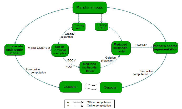
LSMOS is based on Karhunen-Loève expansion (KLE) [27] and can extract most important information from a set of snapshots. When it is difficult to get the knowledge of a covariance function for the model’s ouputs, we can use method of snapshots [21] to construct a KL expansion for the model’s outputs. In LSMOS, the coefficient functions of random variables in the KLE are the functions of the random parameters of inputs. We can use orthogonal polynomial basis functions to express the coefficient functions of the random variables. To determine the coordinates of the orthogonal polynomial basis functions, we take a few snapshots and use least-squares methods. If the dimension of the random parameters is high, a large number of snapshots are required for the least-squares methods. Thus, the computation may be expensive. To overcome the difficulty, we here propose a sparse tensor approximation method to obtain a sparse representation of the model’s outputs instead of using LSMOS. The sparse tensor approximation exploits the inherent sparsity of the model and the reduced GMsFE basis. The number of the effective basis functions for many practical models is often small. We use the optimization methods from compressive sensing [31] to extract the effective basis functions and obtain a sparse representation. There are roughly two classes of approaches to obtain the sparse representation: optimization based on l0subscript𝑙0l_{0}-norm and convex optimization [33, 18, 31]. The typical methods of the l0subscript𝑙0l_{0} optimization include orthogonal matching pursuit (OMP) and iterative hard thresholding. The convex optimization based on l1subscript𝑙1l_{1}-norm includes least angle regression, coordinate descent and proximal methods. In this work, we get the sparse tensor approximation using orthogonal matching pursuit, i.e., STAOMP. We integrate the reduced mixed GMsFE basis methods and STAOMP together to get the model’s sparse representation in coarse scale. The proposed model’s sparse representation method can significantly enhance the computation efficiency for the multiscale models with high-dimensional random inputs. The Figure 1.1 illustrates the procedure to get the model’s sparse representation based on reduced mixed GMsFE basis methods.
Refer to caption
Figure 1.1: Schema of model’s sparse representation based on reduced mixed GMsFE basis methods

The paper is organized as follows. In the next section, we give some preliminaries and notations for the paper. Section 3 is devoted to developing LSMOS and STAOPM to represent a generic random field. In Section 4, we present the construction of the mixed GMsFE basis functions and introduce the reduced mixed GMsFE basis methods. Section 5 is to present two approaches for constructing the optimal reduced basis: BOCV and POD. In Section 6, we combine STAOMP with the reduced mixed GMsFE basis methods together and get the model’s sparse representation. A few numerical examples are provided in Section 7 to illustrate the performance of all the methods developed above. In the last section, we make some comments and conclusions.

2 Preliminaries and notations

In this section, we present some preliminaries and notations for the rest of paper. Let L2(D)superscript𝐿2𝐷L^{2}(D) be the space of square integrable functions over a domain D𝐷D with the L2superscript𝐿2L^{2}-norm L2(D)2=(,)\|\cdot\|_{L^{2}(D)}^{2}=(\cdot,\cdot). We define the space

V:=H(div,D)={u[L2(D)]d:div(u)L2(D)}.assign𝑉𝐻div𝐷conditional-set𝑢superscriptdelimited-[]superscript𝐿2𝐷𝑑div𝑢superscript𝐿2𝐷V:=H(\text{div},D)=\big{\{}u\in[L^{2}(D)]^{d}:\text{div}(u)\in L^{2}(D)\big{\}}.

The space V𝑉V is a Hilbert space with the norm given by uH(div,D)2=uL2(D)2+div(u)L2(D)2superscriptsubscriptnorm𝑢𝐻div𝐷2superscriptsubscriptnorm𝑢superscript𝐿2𝐷2superscriptsubscriptnormdiv𝑢superscript𝐿2𝐷2\|u\|_{H(\text{div},D)}^{2}=\|u\|_{L^{2}(D)}^{2}+\|\text{div}(u)\|_{L^{2}(D)}^{2}. We consider parameterized elliptic PDEs in mixed formulation (1.1) with the Neumann boundary condition kpn=g𝑘𝑝𝑛𝑔k\nabla p\cdot n=g on D𝐷\partial D, where n𝑛n is the outward unit-normal vector on D𝐷\partial D. For a simplicity of notation, we denote L2(D)superscript𝐿2𝐷L^{2}(D) by Q𝑄Q and

V0=H0(div,D):={uH(div,D):un=0onD}.superscript𝑉0subscript𝐻0div𝐷assignconditional-set𝑢𝐻div𝐷𝑢𝑛0on𝐷V^{0}=H_{0}(\text{div},D):=\big{\{}u\in H(\text{div},D):u\cdot n=0~{}\text{on}~{}\partial D\big{\}}.

The problem (1.1) leads to the variational problem: for any parameter μΓp𝜇Γsuperscript𝑝\mu\in\Gamma\subset\mathbb{R}^{p}, we find {v(μ),p(μ)}V×Q𝑣𝜇𝑝𝜇𝑉𝑄\{v(\mu),p(\mu)\}\in V\times Q such that v(μ)n=g𝑣𝜇𝑛𝑔v(\mu)\cdot n=g on D𝐷\partial D,

{a(v(μ),u;μ)b(u,p(μ);μ)=0uV0,b(v(μ),q;μ)=l(q)qQ.casesformulae-sequence𝑎𝑣𝜇𝑢𝜇𝑏𝑢𝑝𝜇𝜇0for-all𝑢superscript𝑉0𝑏𝑣𝜇𝑞𝜇𝑙𝑞for-all𝑞𝑄otherwise\displaystyle\begin{cases}\begin{split}a\big{(}v(\mu),u;\mu\big{)}-b\big{(}u,p(\mu);\mu\big{)}&=0~{}~{}~{}\forall~{}u\in V^{0},\\ b\big{(}v(\mu),q;\mu\big{)}&=l(q)~{}~{}~{}\forall~{}q\in Q.\end{split}\end{cases} (2.2)

where

a(v,w):=Dk(x,μ)1(vw)𝑑x,b(v,w):=D(v)q𝑑x,andl(q):=Dfq𝑑x.formulae-sequenceassign𝑎𝑣𝑤subscript𝐷𝑘superscript𝑥𝜇1𝑣𝑤differential-d𝑥formulae-sequenceassign𝑏𝑣𝑤subscript𝐷𝑣𝑞differential-d𝑥assignand𝑙𝑞subscript𝐷𝑓𝑞differential-d𝑥a(v,w):=\int_{D}k(x,\mu)^{-1}(v\cdot w)dx,~{}~{}b(v,w):=\int_{D}\nabla\cdot(v)qdx,~{}~{}\text{and}~{}~{}l(q):=\int_{D}fqdx.

For any parameter μΓ𝜇Γ\mu\in\Gamma, a(,;μ):V×V:𝑎𝜇𝑉𝑉a(\cdot,\cdot;\mu):V\times V\longrightarrow\mathbb{R} is a symmetric bilinear form , b(,;μ):V×Q:𝑏𝜇𝑉𝑄b(\cdot,\cdot;\mu):V\times Q\longrightarrow\mathbb{R} is bilinear form, and l(;μ)𝑙𝜇l(\cdot;\mu) is a bounded linear functional over Q𝑄Q. Given μΓ𝜇Γ\mu\in\Gamma, we evaluate the output G(x,μ)𝐺𝑥𝜇G(x,\mu) of the model (2.2),

G(x,μ)=L(v(x,μ)),𝐺𝑥𝜇𝐿𝑣𝑥𝜇\displaystyle G(x,\mu)=L\big{(}v(x,\mu)\big{)},

where L𝐿L is a operator on V𝑉V.

For well-posedness of (2.2), we assume that a(,;μ)𝑎𝜇a(\cdot,\cdot;\mu) is continuous and coercive over V𝑉V for all μΓ𝜇Γ\mu\in\Gamma, i.e., there exist γ>0𝛾0\gamma>0 and α>0𝛼0\alpha>0 such that

γ(μ):=supuVsupvVa(u,v;μ)uVvV<,μΓ,formulae-sequenceassign𝛾𝜇subscriptsupremum𝑢𝑉subscriptsupremum𝑣𝑉𝑎𝑢𝑣𝜇subscriptnorm𝑢𝑉subscriptnorm𝑣𝑉for-all𝜇Γ\displaystyle\gamma(\mu):=\sup_{u\in V}\sup_{v\in V}\frac{a(u,v;\mu)}{\|u\|_{V}\|v\|_{V}}<\infty,~{}~{}~{}\forall\mu\in\Gamma, (2.3)
α(μ):=infuVa(u,u;μ)uV2>0,μΓ,formulae-sequenceassign𝛼𝜇subscriptinfimum𝑢𝑉𝑎𝑢𝑢𝜇superscriptsubscriptnorm𝑢𝑉20for-all𝜇Γ\displaystyle\alpha(\mu):=\inf_{u\in V}\frac{a(u,u;\mu)}{\|u\|_{V}^{2}}>0,~{}~{}~{}\forall\mu\in\Gamma, (2.4)

and b(,;μ)𝑏𝜇b(\cdot,\cdot;\mu) is continuous

b(u,q)γbuVqQ,uV,qQ,μΓ,formulae-sequence𝑏𝑢𝑞subscript𝛾𝑏subscriptnorm𝑢𝑉subscriptnorm𝑞𝑄formulae-sequencefor-all𝑢𝑉formulae-sequence𝑞𝑄for-all𝜇Γ\displaystyle b(u,q)\leq\gamma_{b}\|u\|_{V}\|q\|_{Q},\quad\forall u\in V,~{}q\in Q,~{}~{}\forall\mu\in\Gamma,

and satisfies the inf-sup condition

β(μ):=infqQsupuVb(u,q;μ)uVqQ>0,μΓ.formulae-sequenceassign𝛽𝜇subscriptinfimum𝑞𝑄subscriptsupremum𝑢𝑉𝑏𝑢𝑞𝜇subscriptnorm𝑢𝑉subscriptnorm𝑞𝑄0for-all𝜇Γ\displaystyle\beta(\mu):=\inf_{q\in Q}\sup_{u\in V}\frac{b(u,q;\mu)}{\|u\|_{V}\|q\|_{Q}}>0,~{}\forall\mu\in\Gamma. (2.5)

To fulfill offline-online computation, we assume that the parametric bilinear form a(,;μ)𝑎𝜇a(\cdot,\cdot;\mu) is affine with respect to μ𝜇\mu, i.e.,

a(u,v;μ)𝑎𝑢𝑣𝜇\displaystyle a(u,v;\mu) =i=1maki(μ)ai(u,v),u,vV,μΓ,formulae-sequenceabsentsuperscriptsubscript𝑖1subscript𝑚𝑎superscript𝑘𝑖𝜇superscript𝑎𝑖𝑢𝑣for-all𝑢formulae-sequence𝑣𝑉for-all𝜇Γ\displaystyle=\sum_{i=1}^{m_{a}}k^{i}(\mu)a^{i}(u,v),\quad\forall u,v\in V,\quad\forall\mu\in\Gamma, (2.6)

where ki:Γ:superscript𝑘𝑖Γk^{i}:\Gamma\longrightarrow\mathbb{R} is a μ𝜇\mu-dependent function and ai:V×V:superscript𝑎𝑖𝑉𝑉a^{i}:V\times V\longrightarrow\mathbb{R} is a symmetric bilinear form independent of μ𝜇\mu, for each i=1,,ma𝑖1subscript𝑚𝑎i=1,\cdots,m_{a}. The affine assumption (2.6) is crucial to achieve the decomposition of offline-online computation for many queries to model’s outputs. When a(,;μ)𝑎𝜇a(\cdot,\cdot;\mu) is not affine with regard to μ𝜇\mu, such an expansion can be obtained by using some variable separation methods for a(,;μ)𝑎𝜇a(\cdot,\cdot;\mu), e.g., EIM [17], LSMOS and STAOMP. The LSMOS and STAOMP will be introduced in Section 3.

Let Vh×Qhsubscript𝑉subscript𝑄V_{h}\times Q_{h} be the pair of standard Raviart-Thomas space for the approximation of (2.2) on a fine grid 𝒦hsuperscript𝒦\mathcal{K}^{h}. Then the standard mixed FEM of problem (2.2) reads: given any μΓ𝜇Γ\mu\in\Gamma, we find {vh(μ),ph(μ)}Vh×Qhsubscript𝑣𝜇subscript𝑝𝜇subscript𝑉subscript𝑄\{v_{h}(\mu),p_{h}(\mu)\}\in V_{h}\times Q_{h} such that

{a(vh(μ),u;μ)b(u,ph(μ);μ)=0uVh0,b(vh(μ),q;μ)=l(q)qQh,casesformulae-sequence𝑎subscript𝑣𝜇𝑢𝜇𝑏𝑢subscript𝑝𝜇𝜇0for-all𝑢superscriptsubscript𝑉0𝑏subscript𝑣𝜇𝑞𝜇𝑙𝑞for-all𝑞subscript𝑄otherwise\displaystyle\begin{cases}\begin{split}a(v_{h}(\mu),u;\mu)-b(u,p_{h}(\mu);\mu)&=0~{}~{}~{}\forall~{}u\in V_{h}^{0},\\ b(v_{h}(\mu),q;\mu)&=l(q)~{}~{}~{}\forall~{}q\in Q_{h},\end{split}\end{cases} (2.7)

where Vh0=Vh{vVh:vn=0onD}superscriptsubscript𝑉0subscript𝑉conditional-set𝑣subscript𝑉𝑣𝑛0on𝐷V_{h}^{0}=V_{h}\bigcap\{v\in V_{h}:v\cdot n=0~{}\text{on}~{}\partial D\}. We remark that the fine-grid solution is considered as a reference solution in the paper.

3 Variable-separation strategies

In order to achieve offline-online computation, we want to represent model’s inputs (e.g., coefficients and source terms) and outputs by a form of variable-separation. Let G(x,μ)𝐺𝑥𝜇G(x,\mu) be a generic function parameterized by μ𝜇\mu. In this section, we introduce two strategies, i.e., LSMOS and STAOMP, to construct an approximation in the form

G(x,μ)GN(x,μ):=i=1Nζi(μ)gi(x),𝐺𝑥𝜇subscript𝐺𝑁𝑥𝜇assignsuperscriptsubscript𝑖1𝑁subscript𝜁𝑖𝜇subscript𝑔𝑖𝑥\displaystyle G(x,\mu)\approx G_{N}(x,\mu):=\sum_{i=1}^{N}\zeta_{i}(\mu)g_{i}(x), (3.8)

where ζi(μ)subscript𝜁𝑖𝜇\zeta_{i}(\mu) only depends on μ𝜇\mu and gi(x)subscript𝑔𝑖𝑥g_{i}(x) only depends on x𝑥x. Let L2(Γ)subscript𝐿2ΓL_{2}(\Gamma) be the space of square integrable functions over the parameter space ΓΓ\Gamma. We consider the approximation in the tensor space L2(Γ)tensor-productsubscript𝐿2Γ\mathcal{H}\otimes L_{2}(\Gamma), where \mathcal{H} is a Hilbert space with regard to the spatial space. We define an inner product on L2(Γ)tensor-productsubscript𝐿2Γ\mathcal{H}\otimes L_{2}(\Gamma) by

(w,u)L2(Γ)=E[(w,u)]:=Γ(w,u)ρ(μ)𝑑μ,subscript𝑤𝑢tensor-productsubscript𝐿2Γ𝐸delimited-[]subscript𝑤𝑢assignsubscriptΓsubscript𝑤𝑢𝜌𝜇differential-d𝜇\displaystyle(w,u)_{\mathcal{H}\otimes L_{2}(\Gamma)}=E[(w,u)_{\mathcal{H}}]:=\int_{\Gamma}(w,u)_{\mathcal{H}}\rho(\mu)d\mu,

where ρ(μ)𝜌𝜇\rho(\mu) is the density function for the random parameter μ𝜇\mu. The norm is defined by

uL2(Γ)2:=(u,u)L2(Γ).assignsuperscriptsubscriptnorm𝑢tensor-productsubscript𝐿2Γ2subscript𝑢𝑢tensor-productsubscript𝐿2Γ\|u\|_{\mathcal{H}\otimes L_{2}(\Gamma)}^{2}:=(u,u)_{\mathcal{H}\otimes L_{2}(\Gamma)}.

We assume that SNL2(Γ)subscript𝑆𝑁tensor-productsubscript𝐿2ΓS_{N}\subset\mathcal{H}\otimes L_{2}(\Gamma) is a finite dimensional subspace space, and {Ψi}i=1NsuperscriptsubscriptsubscriptΨ𝑖𝑖1𝑁\{\Psi_{i}\}_{i=1}^{N} is a set of basis functions for SNsubscript𝑆𝑁S_{N}. We want to find an approximation of G(x,μ)𝐺𝑥𝜇G(x,\mu) in SNsubscript𝑆𝑁S_{N} such that

G(x,μ)j=1NcjΨj(x,μ)L2(Γ)δ,subscriptnorm𝐺𝑥𝜇superscriptsubscript𝑗1𝑁subscript𝑐𝑗subscriptΨ𝑗𝑥𝜇tensor-productsubscript𝐿2Γ𝛿\displaystyle\|G(x,\mu)-\sum_{j=1}^{N}c_{j}\Psi_{j}(x,\mu)\|_{\mathcal{H}\otimes L_{2}(\Gamma)}\leq\delta, (3.9)

where δ𝛿\delta is a given threshold.

3.1 Least-squares method of snapshots

In this subsection, we introduce a least-squares method of snapshots to get the approximation (3.9). Let ΞtsubscriptΞ𝑡\Xi_{t} be a collection of a finite number of samples in ΓΓ\Gamma and the cardinality |Ξt|=ntsubscriptΞ𝑡subscript𝑛𝑡|\Xi_{t}|=n_{t}. For μΞtfor-all𝜇subscriptΞ𝑡\forall~{}\mu\in\Xi_{t}, we can split G(x,μ)𝐺𝑥𝜇G(x,\mu) into two parts, i.e.,

G(x,μ)=G¯(x)+G~(x,μ),𝐺𝑥𝜇¯𝐺𝑥~𝐺𝑥𝜇G(x,\mu)=\bar{G}(x)+\tilde{G}(x,\mu),

where G¯(x):=E[G(x,)]=1nti=1ntG(x,μi)assign¯𝐺𝑥𝐸delimited-[]𝐺𝑥1subscript𝑛𝑡superscriptsubscript𝑖1subscript𝑛𝑡𝐺𝑥subscript𝜇𝑖\bar{G}(x):=E[G(x,\cdot)]=\frac{1}{n_{t}}\sum_{i=1}^{n_{t}}G(x,\mu_{i}) is the mean, and G~(x,μ)=G(x,μ)G¯(x)~𝐺𝑥𝜇𝐺𝑥𝜇¯𝐺𝑥\tilde{G}(x,\mu)=G(x,\mu)-\bar{G}(x) is a random fluctuating part. To obtain G~(x,μ)~𝐺𝑥𝜇\tilde{G}(x,\mu), we take a set of snapshots {G~(x,μi)}i=1ntsuperscriptsubscript~𝐺𝑥subscript𝜇𝑖𝑖1subscript𝑛𝑡\{\tilde{G}(x,\mu_{i})\}_{i=1}^{n_{t}} and compute a covariance matrixes C, whose entries can be defined by

Cn,m:=1nt(G~(x,μn),G~(x,μm)).assignsubscriptC𝑛𝑚1subscript𝑛𝑡subscript~𝐺𝑥subscript𝜇𝑛~𝐺𝑥subscript𝜇𝑚\textbf{C}_{n,m}:=\frac{1}{n_{t}}\bigg{(}\tilde{G}(x,\mu_{n}),\tilde{G}(x,\mu_{m})\bigg{)}_{\mathcal{H}}.

Let {λ^k,ek}subscript^𝜆𝑘subscripte𝑘\{\hat{\lambda}_{k},\textbf{e}_{k}\} be the eigen-pairs (normalized) of C, 1knt1𝑘subscript𝑛𝑡1\leq k\leq n_{t}. Set (ek)j=ekjsubscriptsubscripte𝑘𝑗superscriptsubscript𝑒𝑘𝑗(\textbf{e}_{k})_{j}=e_{k}^{j}, we define the functions

gk(x):=1λ^kntj=1ntekjG~(x,μj).assignsubscript𝑔𝑘𝑥1subscript^𝜆𝑘subscript𝑛𝑡superscriptsubscript𝑗1subscript𝑛𝑡superscriptsubscript𝑒𝑘𝑗~𝐺𝑥subscript𝜇𝑗\displaystyle g_{k}(x):=\frac{1}{\sqrt{\hat{\lambda}_{k}n_{t}}}\sum_{j=1}^{n_{t}}e_{k}^{j}\tilde{G}(x,\mu_{j}). (3.10)

It is easy to get (gk,gl)=δk,lsubscriptsubscript𝑔𝑘subscript𝑔𝑙subscript𝛿𝑘𝑙(g_{k},g_{l})_{\mathcal{H}}=\delta_{k,l}, 1k1𝑘1\leq k, lnt𝑙subscript𝑛𝑡l\leq n_{t}. Then it holds that

G~(x,μ)i=1ntλ^iζi(μ)gi(x),~𝐺𝑥𝜇superscriptsubscript𝑖1subscript𝑛𝑡subscript^𝜆𝑖subscript𝜁𝑖𝜇subscript𝑔𝑖𝑥\tilde{G}(x,\mu)\approx\sum_{i=1}^{n_{t}}\sqrt{\hat{\lambda}_{i}}\zeta_{i}(\mu)g_{i}(x),

where {ζi(μ)}i=1ntsuperscriptsubscriptsubscript𝜁𝑖𝜇𝑖1subscript𝑛𝑡\{\zeta_{i}(\mu)\}_{i=1}^{n_{t}} are given by

ζi(μ):=1λ^i(G~(,μ),gi).assignsubscript𝜁𝑖𝜇1subscript^𝜆𝑖subscript~𝐺𝜇subscript𝑔𝑖\displaystyle\begin{split}\zeta_{i}(\mu):=\frac{1}{\sqrt{\hat{\lambda}_{i}}}\big{(}\tilde{G}(\cdot,\mu),g_{i}\big{)}_{\mathcal{H}}.\end{split} (3.11)

Thus we get the decomposition

G(x,μ)G¯(x)+i=1Mλ^iζi(μ)gi(x).𝐺𝑥𝜇¯𝐺𝑥superscriptsubscript𝑖1𝑀subscript^𝜆𝑖subscript𝜁𝑖𝜇subscript𝑔𝑖𝑥\displaystyle G(x,\mu)\approx\bar{G}(x)+\sum_{i=1}^{M}\sqrt{\hat{\lambda}_{i}}\zeta_{i}(\mu)g_{i}(x). (3.12)

Because the equation (3.11) involves G~(,μ)~𝐺𝜇\tilde{G}(\cdot,\mu), it can not be directly used to compute the functions {ζi(μ)}i=1ntsuperscriptsubscriptsubscript𝜁𝑖𝜇𝑖1subscript𝑛𝑡\{\zeta_{i}(\mu)\}_{i=1}^{n_{t}} for arbitrary μ𝜇\mu. We will apply least-squares methods to approximate {ζi(μ)}i=1ntsuperscriptsubscriptsubscript𝜁𝑖𝜇𝑖1subscript𝑛𝑡\{\zeta_{i}(\mu)\}_{i=1}^{n_{t}} based on orthogonal polynomials. Let {pi(μ)}i=1Mgsuperscriptsubscriptsubscript𝑝𝑖𝜇𝑖1subscript𝑀𝑔\{p_{i}(\mu)\}_{i=1}^{M_{g}} be the set of orthogonal polynomials basis functions with total degree less than Ngsubscript𝑁𝑔N_{g} regarding to the parameter variable μ𝜇\mu. We rearrange the set of basis functions from the first to the last one and place them in the following row vector,

[p1(μ),p2(μ),,pMg(μ)],whereMg=(Ng+pNg).subscript𝑝1𝜇subscript𝑝2𝜇subscript𝑝subscript𝑀𝑔𝜇wheresubscript𝑀𝑔subscript𝑁𝑔𝑝missing-subexpressionsubscript𝑁𝑔missing-subexpression\big{[}p_{1}(\mu),p_{2}(\mu),...,p_{M_{g}}(\mu)\big{]},~{}~{}~{}~{}\text{where}~{}~{}M_{g}=\left(\begin{array}[]{cc}N_{g}+p\\ N_{g}\\ \end{array}\right).

For the sample date ΞtsubscriptΞ𝑡\Xi_{t}, we compute [p1(μj),p2(μj),,pMg(μj)]subscript𝑝1subscript𝜇𝑗subscript𝑝2subscript𝜇𝑗subscript𝑝subscript𝑀𝑔subscript𝜇𝑗[p_{1}(\mu_{j}),p_{2}(\mu_{j}),\cdots,p_{M_{g}}(\mu_{j})] and ζi(μj)=1λ^i(G~(,μj),gi)subscript𝜁𝑖subscript𝜇𝑗1subscript^𝜆𝑖subscript~𝐺subscript𝜇𝑗subscript𝑔𝑖\zeta_{i}(\mu_{j})=\frac{1}{\sqrt{\hat{\lambda}_{i}}}(\tilde{G}(\cdot,\mu_{j}),g_{i})_{\mathcal{H}} (j=1,,nt𝑗1subscript𝑛𝑡j=1,\cdots,n_{t}). They are putted in the following matrix A and vector F , respectively,

A:=[p1(μ1)pMg(μ1)p1(μnt)pMg(μnt)],assignAdelimited-[]subscript𝑝1subscript𝜇1subscript𝑝subscript𝑀𝑔subscript𝜇1subscript𝑝1subscript𝜇subscript𝑛𝑡subscript𝑝subscript𝑀𝑔subscript𝜇subscript𝑛𝑡\displaystyle\textbf{A}:=\left[\begin{array}[]{ccc}p_{1}(\mu_{1})&\ldots&p_{M_{g}}(\mu_{1})\\ \vdots&\ddots&\vdots\\ p_{1}(\mu_{n_{t}})&\ldots&p_{M_{g}}(\mu_{n_{t}})\\ \end{array}\right], (3.16)
F:=[ζi(μ1)ζi(μnt)]T.assignFsuperscriptdelimited-[]subscript𝜁𝑖subscript𝜇1subscript𝜁𝑖subscript𝜇subscript𝑛𝑡𝑇\displaystyle\textbf{F}:=[\zeta_{i}(\mu_{1})\cdots\zeta_{i}(\mu_{n_{t}})]^{T}. (3.17)

We obtain the approximation of the parameter functions ζi(μ)subscript𝜁𝑖𝜇\zeta_{i}(\mu) by solving the following least square problem,

d=argminαAαF2.dsubscript𝛼subscriptdelimited-∥∥A𝛼F2\displaystyle\begin{split}\textbf{d}=\arg\min_{\alpha}\|\textbf{A}\alpha-\textbf{F}\|_{2}.\end{split} (3.18)

Thus we get ζi(μ)i=1Mgdipi(μ)subscript𝜁𝑖𝜇superscriptsubscript𝑖1subscript𝑀𝑔subscript𝑑𝑖subscript𝑝𝑖𝜇\zeta_{i}(\mu)\approx\sum_{i=1}^{M_{g}}d_{i}p_{i}(\mu), and di=(d)isubscript𝑑𝑖subscriptd𝑖d_{i}=(\textbf{d})_{i}.

3.2 Sparse tensor approximation

In this subsection, we are devote to seeking the optimal solution c for (3.9) with the minimum number of non-zero terms. This can be formulated as the optimization problem:

argmincc0subject toG(x,μ)j=1NcjΨj(x,μ)L2(Γ)δ,subscriptcsubscriptnormc0subject tosubscriptnorm𝐺𝑥𝜇superscriptsubscript𝑗1𝑁subscript𝑐𝑗subscriptΨ𝑗𝑥𝜇tensor-productsubscript𝐿2Γ𝛿\displaystyle\arg\min_{\textbf{c}}\|\textbf{c}\|_{0}~{}~{}\text{subject to}~{}~{}\|G(x,\mu)-\sum_{j=1}^{N}c_{j}\Psi_{j}(x,\mu)\|_{\mathcal{H}\otimes L_{2}(\Gamma)}\leq\delta, (3.19)

where

c=(c1,,cN),andc0={j:cj0}.formulae-sequencecsubscript𝑐1subscript𝑐𝑁andsubscriptnormc0conditional-set𝑗subscript𝑐𝑗0\textbf{c}=(c_{1},\cdots,c_{N}),\quad\text{and}\quad\|\textbf{c}\|_{0}=\sharp\{j:c_{j}\neq 0\}.

Thus the sparse solution can be constructed as follows.
\bullet Step 1: Find the optimal N𝑁N-dimensional subspace Nsubscript𝑁\mathcal{H}_{N}\subseteq\mathcal{H}

With the snapshots {G(x,μi)}i=1ntsuperscriptsubscript𝐺𝑥subscript𝜇𝑖𝑖1subscript𝑛𝑡\{G(x,\mu_{i})\}_{i=1}^{n_{t}}, we can use methods of snapshots or POD to construct the optimal N𝑁N-dimensional subspace

N=span{gj(x):1jN}.subscript𝑁spanconditional-setsubscript𝑔𝑗𝑥1𝑗𝑁\mathcal{H}_{N}=\text{span}\big{\{}g_{j}(x):1\leq j\leq N\big{\}}.

\bullet Step 2: Choose orthogonal polynomials for L2(Γ)subscript𝐿2ΓL_{2}(\Gamma) and construct the finite dimensional approximation space SN×ML2(Γ)subscript𝑆𝑁𝑀tensor-productsubscript𝐿2ΓS_{N\times M}\subseteq\mathcal{H}\otimes L_{2}(\Gamma)

For the parameter, we introduce appoximation spaces XMsubscript𝑋𝑀X_{M} for L2(Γ)subscript𝐿2ΓL_{2}(\Gamma),

XM=span{pi(μ):1iM}.subscript𝑋𝑀spanconditional-setsubscript𝑝𝑖𝜇1𝑖𝑀X_{M}=\text{span}\big{\{}p_{i}(\mu):1\leq i\leq M\big{\}}.

A finite dimensional approximation space SN×ML2(Γ)subscript𝑆𝑁𝑀tensor-productsubscript𝐿2ΓS_{N\times M}\subseteq\mathcal{H}\otimes L_{2}(\Gamma) is then obtained by

SN×M:=NXM=span{pi(μ)gj(x):1iM,1jN}.assignsubscript𝑆𝑁𝑀tensor-productsubscript𝑁subscript𝑋𝑀spanconditional-setsubscript𝑝𝑖𝜇subscript𝑔𝑗𝑥formulae-sequence1𝑖𝑀1𝑗𝑁S_{N\times M}:=\mathcal{H}_{N}\otimes X_{M}=\text{span}\big{\{}p_{i}(\mu)g_{j}(x):1\leq i\leq M,1\leq j\leq N\big{\}}.

To simplify notation, we use the following single-index notation

SN×M={w(x,μ)=iIwiΨi(x,μ);wi},subscript𝑆𝑁𝑀formulae-sequence𝑤𝑥𝜇subscript𝑖𝐼subscript𝑤𝑖subscriptΨ𝑖𝑥𝜇subscript𝑤𝑖S_{N\times M}=\big{\{}w(x,\mu)=\sum_{i\in I}w_{i}\Psi_{i}(x,\mu);~{}w_{i}\in\mathbb{R}\big{\}},

where I={1,,N}×{1,,M}𝐼1𝑁1𝑀I=\{1,\cdots,N\}\times\{1,\cdots,M\} and Ψi(x,μ)=pi1(μ)ui2(x)subscriptΨ𝑖𝑥𝜇subscript𝑝subscript𝑖1𝜇subscript𝑢subscript𝑖2𝑥\Psi_{i}(x,\mu)=p_{i_{1}}(\mu)u_{i_{2}}(x).
\bullet Step 3: Construct the sparse solution based on Orthogonal-Matching-Pursuit

In general, the optimization problem (3.19) is an NP-hard problem. We attempt to seek efficient algorithms to approximately solve (3.19). There are a few approaches [31] to solve the problem (3.19). In the paper, we focus on Orthogonal Matching Pursuit (OMP) algorithm [33] to get a sparse solution.

We place the basis functions {Ψi(x,μ)}i=1M×NSN×MsuperscriptsubscriptsubscriptΨ𝑖𝑥𝜇𝑖1𝑀𝑁subscript𝑆𝑁𝑀\{\Psi_{i}(x,\mu)\}_{i=1}^{M\times N}\subseteq S_{N\times M} in the following row vector,

Ψ:=[Ψ1,Ψ2,,ΨM×N].assignΨsubscriptΨ1subscriptΨ2subscriptΨ𝑀𝑁\Psi:=[\Psi_{1},\Psi_{2},\cdots,\Psi_{M\times N}].

Assume that n=nx×nμ𝑛subscript𝑛𝑥subscript𝑛𝜇n=n_{x}\times n_{\mu} sample data {(xi,μj)}D×Γsubscript𝑥𝑖subscript𝜇𝑗𝐷Γ\{(x_{i},\mu_{j})\}\subseteq D\times\Gamma (1inx1𝑖subscript𝑛𝑥1\leq i\leq n_{x}, 1jnμ1𝑗subscript𝑛𝜇1\leq j\leq n_{\mu}) are chosen to solve the optimization problem (3.19). For the sample date, we compute Ψ(xi,μj)Ψsubscript𝑥𝑖subscript𝜇𝑗\Psi(x_{i},\mu_{j}) and G(xi,μj)𝐺subscript𝑥𝑖subscript𝜇𝑗G(x_{i},\mu_{j}), and they are putted in the following matrix Πn×(M×N)Πsuperscript𝑛𝑀𝑁\Pi\in\mathbb{R}^{n\times(M\times N)} and vector bn×1bsuperscript𝑛1\textbf{b}\in\mathbb{R}^{n\times 1}, respectively,

Π:=[Ψ1(x1,μ1)ΨM×N(x1,μ1)Ψ1(xnx,μnμ)ΨM×N(xnx,μnμ)],b:=[G(x1,μ1)G(xnx,μnμ)].formulae-sequenceassignΠdelimited-[]subscriptΨ1subscript𝑥1subscript𝜇1subscriptΨ𝑀𝑁subscript𝑥1subscript𝜇1subscriptΨ1subscript𝑥subscript𝑛𝑥subscript𝜇subscript𝑛𝜇subscriptΨ𝑀𝑁subscript𝑥subscript𝑛𝑥subscript𝜇subscript𝑛𝜇assignbdelimited-[]𝐺subscript𝑥1subscript𝜇1missing-subexpressionmissing-subexpressionmissing-subexpressionmissing-subexpression𝐺subscript𝑥subscript𝑛𝑥subscript𝜇subscript𝑛𝜇missing-subexpressionmissing-subexpression\displaystyle\Pi:=\left[\begin{array}[]{ccc}\Psi_{1}(x_{1},\mu_{1})&\ldots&\Psi_{M\times N}(x_{1},\mu_{1})\\ \vdots&\ddots&\vdots\\ \Psi_{1}(x_{n_{x}},\mu_{n_{\mu}})&\ldots&\Psi_{M\times N}(x_{n_{x}},\mu_{n_{\mu}})\\ \end{array}\right],~{}~{}~{}~{}\textbf{b}:=\left[\begin{array}[]{ccc}G(x_{1},\mu_{1})\\ \vdots\\ G(x_{n_{x}},\mu_{n_{\mu}})\\ \end{array}\right]. (3.26)

The coefficient vector can be solved by the following optimization problem,

argmincc0subject tobΠc2δ.subscriptcsubscriptnormc0subject tosubscriptnormbΠc2𝛿\displaystyle\arg\min_{\textbf{c}}\|\textbf{c}\|_{0}~{}~{}\text{subject to}~{}~{}\|\textbf{b}-\Pi\textbf{c}\|_{2}\leq\delta. (3.27)

The main idea of OMP is to pick columns in a greedy manner. At each iteration, we choose the column of ΠΠ\Pi that is most strongly correlated with the remaining part of b, i.e., the residual rksubscriptr𝑘\textbf{r}_{k} in Algorithm 1. Then we subtract off the contribution to b and iterate with regard to the updated residual. After k𝑘k iterations, the algorithm can identify the correct set of columns. The OMP is described in Algorithm 1.

Algorithm 1 Orthogonal-Matching-Pursuit

Input: A matrix ΠΠ\Pi, the vector b and the error tolerance ε𝜀\varepsilon
Output: The sparse solution c and the solution support I:=supp(c)assignI𝑠𝑢𝑝𝑝c\emph{I}:=supp(\textbf{c})
 1:  Initialize the residual r0=bsubscriptr0b\textbf{r}_{0}=\textbf{b}, the index set I0=ØsuperscriptI0italic-Ø\emph{I}^{0}={\O}, the iteration counter k=1𝑘1k=1, and
Π0subscriptΠ0~{}~{}~{}~{}~{}\Pi_{0} is an empty matrix;
 2:  Find the index j0subscript𝑗0j_{0} that solves the easy optimization problem:
j0=argmaxj=1,,M×N|rk,Ψj|subscript𝑗0subscript𝑗1𝑀𝑁subscriptr𝑘subscriptΨ𝑗~{}~{}~{}~{}~{}j_{0}=\arg\max_{j=1,...,M\times N}|\langle\textbf{r}_{k},\Psi_{j}\rangle|;
 3:  Update the index set Ik=Ik1{j0}superscriptI𝑘superscriptI𝑘1subscript𝑗0\emph{I}^{k}=\emph{I}^{k-1}\cup\{j_{0}\}, the matrix Πk=[Πk1Ψj0]subscriptΠ𝑘delimited-[]subscriptΠ𝑘1subscriptΨsubscript𝑗0\Pi_{k}=[\Pi_{k-1}~{}\Psi_{j_{0}}];
 4:  Solve a least-squares problem to obtain a new estimate:
ck=argmincbΠkc2superscriptc𝑘subscriptcsubscriptnormbsubscriptΠ𝑘c2~{}~{}~{}~{}~{}\textbf{c}^{k}=\arg\min_{\textbf{c}}\|\textbf{b}-\Pi_{k}\textbf{c}\|_{2};
 5:  Calculate the new residual: rk=bΠkcksubscriptr𝑘bsubscriptΠ𝑘superscriptc𝑘\textbf{r}_{k}=\textbf{b}-\Pi_{k}\textbf{c}^{k};
 6:  kk+1𝑘𝑘1k\rightarrow k+1, return to Step 2 if rk2bk2εsubscriptnormsubscriptr𝑘2subscriptnormsubscriptb𝑘2𝜀\frac{\|\textbf{r}_{k}\|_{2}}{\|\textbf{b}_{k}\|_{2}}\geq\varepsilon, otherwise terminate .
 7:  Mt=kMt𝑘\text{Mt}=k, I=IkIsuperscriptI𝑘\emph{I}=\emph{I}^{k}, and c=ckcsuperscriptc𝑘\textbf{c}=\textbf{c}^{k}.

The residual is always orthogonal to the columns that have been selected. In fact, we can get the conclusion from step 444 in Algorithm 1 by vanishing the derivative of bΠkc2subscriptnormbsubscriptΠ𝑘c2\|\textbf{b}-\Pi_{k}\textbf{c}\|_{2}, i.e.,

ΠkT(bΠkc)=ΠkTrk=0.superscriptsubscriptΠ𝑘𝑇bsubscriptΠ𝑘csuperscriptsubscriptΠ𝑘𝑇subscriptr𝑘0-\Pi_{k}^{T}(\textbf{b}-\Pi_{k}\textbf{c})=-\Pi_{k}^{T}\textbf{r}_{k}=0.

Thus, OMP never selects the same column twice. Provided that the residual is nonzero, the algorithm selects a new atom at each iteration and the matrix ΠksubscriptΠ𝑘\Pi_{k} has full column rank.

Remark 3.1.

For the classical least-squares method, it is required that the number of parameter sample scales quadratically with the number of unknowns [8]. However, STAOMP can provide an accurate approximation by a much fewer number of samples.

4 Reduced mixed GMsFE basis method

Let 𝒦Hsuperscript𝒦𝐻\mathcal{K}^{H} be a conforming coarse partition for the computational domain D𝐷D, where H𝐻H is the coarse mesh size. Each coarse-grid block is further partitioned into a connected union of fine-grid blocks, we get the fine grid partition 𝒦hsuperscript𝒦\mathcal{K}^{h}. Let εH:=i=1Ne{Ei}assignsuperscript𝜀𝐻superscriptsubscript𝑖1subscript𝑁𝑒subscript𝐸𝑖\varepsilon^{H}:=\bigcup_{i=1}^{N_{e}}\{E_{i}\} be the set of all edges/interfaces of coarse mesh 𝒦Hsuperscript𝒦𝐻\mathcal{K}^{H} and Nesubscript𝑁𝑒N_{e} the number of coarse edges. The coarse neighborhood wisubscript𝑤𝑖w_{i} corresponding to the coarse edge Eisubscript𝐸𝑖E_{i} is defined by

wi={Kj𝒦H;EiKj}.subscript𝑤𝑖formulae-sequencesubscript𝐾𝑗superscript𝒦𝐻subscript𝐸𝑖subscript𝐾𝑗w_{i}=\bigcup\{K_{j}\in\mathcal{K}^{H};E_{i}\in\partial K_{j}\}.

In the mixed GMsFEM, the velocity field is approximated by using mixed GMsFE basis functions, while piecewise constant functions over 𝒦Hsuperscript𝒦𝐻\mathcal{K}^{H} are used to approximate the pressure field. Let QHsubscript𝑄𝐻Q_{H} be the space of piecewise constant functions over the coarse grid 𝒦Hsuperscript𝒦𝐻\mathcal{K}^{H}. Let {ϕj}j=1Lisuperscriptsubscriptsubscriptitalic-ϕ𝑗𝑗1subscript𝐿𝑖\{\phi_{j}\}_{j=1}^{L_{i}} be the set of GMsFE basis functions corresponding to edge Eisubscript𝐸𝑖E_{i}. We define the GMsFE space for the velocity field as the linear span of all local basis functions, i.e.,

VH=εH{ϕj}j=1Li.subscript𝑉𝐻subscriptdirect-sumsuperscript𝜀𝐻superscriptsubscriptsubscriptitalic-ϕ𝑗𝑗1subscript𝐿𝑖V_{H}=\bigoplus_{\varepsilon^{H}}\{\phi_{j}\}_{j=1}^{L_{i}}.

Let VH0=VH{uVH:un=0onD}superscriptsubscript𝑉𝐻0subscript𝑉𝐻conditional-set𝑢subscript𝑉𝐻𝑢𝑛0on𝐷V_{H}^{0}=V_{H}\bigcap\{u\in V_{H}:u\cdot n=0~{}\text{on}~{}\partial D\} be a subspace of VHsubscript𝑉𝐻V_{H}. Thus the mixed GMsFEM is to find {vH(μ),pH(μ)}VH×QHsubscript𝑣𝐻𝜇subscript𝑝𝐻𝜇subscript𝑉𝐻subscript𝑄𝐻\{v_{H}(\mu),p_{H}(\mu)\}\in V_{H}\times Q_{H} such that

{a(vH(μ),u;μ)b(u,pH(μ);μ)=0uVH0,b(vH(μ),q;μ)=l(q)qQH,casesformulae-sequence𝑎subscript𝑣𝐻𝜇𝑢𝜇𝑏𝑢subscript𝑝𝐻𝜇𝜇0for-all𝑢superscriptsubscript𝑉𝐻0𝑏subscript𝑣𝐻𝜇𝑞𝜇𝑙𝑞for-all𝑞subscript𝑄𝐻otherwise\displaystyle\begin{cases}\begin{split}a(v_{H}(\mu),u;\mu)-b(u,p_{H}(\mu);\mu)&=0~{}~{}~{}\forall~{}u\in V_{H}^{0},\\ b(v_{H}(\mu),q;\mu)&=l(q)~{}~{}~{}\forall~{}q\in Q_{H},\\ \end{split}\end{cases} (4.28)

where vH(μ)n=gHonDsubscript𝑣𝐻𝜇𝑛subscript𝑔𝐻on𝐷v_{H}(\mu)\cdot n=g_{H}~{}\text{on}~{}\partial D, and for each coarse edge EiDsubscript𝐸𝑖𝐷E_{i}\in\partial D,

Ei(gHg)ϕjn=0,j=1,,Li.formulae-sequencesubscriptsubscript𝐸𝑖subscript𝑔𝐻𝑔subscriptitalic-ϕ𝑗𝑛0𝑗1subscript𝐿𝑖\int_{E_{i}}(g_{H}-g)\phi_{j}\cdot n=0,~{}j=1,\cdots,L_{i}.

It is easy to see that QHQhsubscript𝑄𝐻subscript𝑄Q_{H}\subset Q_{h} and VHVhsubscript𝑉𝐻subscript𝑉V_{H}\subset V_{h} in the mixed GMsFEM. We will briefly present the mixed GMsFEM and introduce reduced mixed GMsFE basis methods.

4.1 Mixed GMsFE space

In this section, we follow mixed GMsFEM [10] and present the construction of the GMsFE space VHsubscript𝑉𝐻V_{H} for the approximation of the velocity field. We first t generate the snapshot space and then use spectral decomposition to obtain a lower-dimensional offline space.

Let EiεHsubscript𝐸𝑖superscript𝜀𝐻E_{i}\in\varepsilon^{H} be a coarse edge and ejEisubscript𝑒𝑗subscript𝐸𝑖e_{j}\subset E_{i} a fine edge, and define a piecewise constant function δjisuperscriptsubscript𝛿𝑗𝑖\delta_{j}^{i} on Eisubscript𝐸𝑖E_{i} as

δjisuperscriptsubscript𝛿𝑗𝑖\displaystyle\delta_{j}^{i} ={1,onej,0,on other fine edges ofEi.absentcases1onsubscript𝑒𝑗0on other fine edges ofsubscript𝐸𝑖otherwise\displaystyle=\begin{cases}\begin{split}1,&~{}\text{on}~{}e_{j},\\ 0,&~{}\text{on other fine edges of}~{}E_{i}.\end{split}\end{cases}

We solve the following problem on the coarse neighborhood wisubscript𝑤𝑖w_{i} corresponding to the edge Eisubscript𝐸𝑖E_{i},

{k(x,μ)1vji(μ)+pji(μ)=0inwi,vji(μ)=αjiinwi,vji(μ)ni=0onwi,casesformulae-sequence𝑘superscript𝑥𝜇1superscriptsubscript𝑣𝑗𝑖𝜇superscriptsubscript𝑝𝑗𝑖𝜇0insubscript𝑤𝑖formulae-sequencesuperscriptsubscript𝑣𝑗𝑖𝜇superscriptsubscript𝛼𝑗𝑖insubscript𝑤𝑖superscriptsubscript𝑣𝑗𝑖𝜇subscript𝑛𝑖0onsubscript𝑤𝑖otherwise\displaystyle\begin{cases}\begin{split}k(x,\mu)^{-1}v_{j}^{i}(\mu)+\nabla p_{j}^{i}(\mu)&=0~{}~{}\text{in}~{}~{}w_{i},\\ \nabla\cdot v_{j}^{i}(\mu)&=\alpha_{j}^{i}~{}\text{in}~{}~{}w_{i},\\ v_{j}^{i}(\mu)\cdot n_{i}&=0~{}~{}\text{on}~{}~{}\partial w_{i},\end{split}\end{cases} (4.29)

where the constant αjisuperscriptsubscript𝛼𝑗𝑖\alpha_{j}^{i} satisfies the compatibility condition Knαji=Eiδjisubscriptsubscript𝐾𝑛superscriptsubscript𝛼𝑗𝑖subscriptsubscript𝐸𝑖superscriptsubscript𝛿𝑗𝑖\int_{K_{n}}\alpha_{j}^{i}=\int_{E_{i}}\delta_{j}^{i} for all Knwisubscript𝐾𝑛subscript𝑤𝑖K_{n}\subset w_{i}, and nisubscript𝑛𝑖n_{i} denotes the outward unit normal vector on wisubscript𝑤𝑖\partial w_{i}. The local problem (4.29) is solved separately in the coarse-grid blocks of wisubscript𝑤𝑖w_{i}. We need an extra boundary condition on Eisubscript𝐸𝑖E_{i} for well-posedness. Let Jisubscript𝐽𝑖J_{i} be the total number of fine-grid edges on Eisubscript𝐸𝑖E_{i} and Ei=j=1Jiejsubscript𝐸𝑖superscriptsubscript𝑗1subscript𝐽𝑖subscript𝑒𝑗E_{i}=\cup_{j=1}^{J_{i}}e_{j}, where ejsubscript𝑒𝑗e_{j} denotes a fine-grid edge. The remaining boundary condition on the coarse edge Eisubscript𝐸𝑖E_{i} for the local problem (4.29) is taken as

vji(μ)mi=δjionEi,superscriptsubscript𝑣𝑗𝑖𝜇subscript𝑚𝑖superscriptsubscript𝛿𝑗𝑖onsubscript𝐸𝑖\displaystyle v_{j}^{i}(\mu)\cdot m_{i}=\delta_{j}^{i}~{}~{}\text{on}~{}~{}E_{i},

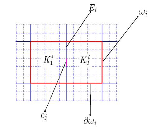
where misubscript𝑚𝑖m_{i} is a fixed unit-normal vector on Eisubscript𝐸𝑖E_{i}. See Figure 4.2 for illustration of a coarse neighborhood. Then we define the snapshot space Vsnapsubscript𝑉𝑠𝑛𝑎𝑝V_{snap} space by

Vsnap=span{vji(μ):1jJi,1iNe}.subscript𝑉𝑠𝑛𝑎𝑝spanconditional-setsuperscriptsubscript𝑣𝑗𝑖𝜇formulae-sequence1𝑗subscript𝐽𝑖1𝑖subscript𝑁𝑒V_{snap}=\text{span}\{v_{j}^{i}(\mu):1\leq j\leq J_{i},1\leq i\leq N_{e}\}.
Refer to caption
Figure 4.2: Illustration of a neighborhood ωi=K1iK2isubscript𝜔𝑖superscriptsubscript𝐾1𝑖superscriptsubscript𝐾2𝑖\omega_{i}=K_{1}^{i}\cup K_{2}^{i}.

After the construction of the snapshot space, the offline space is constructed by performing some local spectral problem on the snapshot space. Let Vsnapisuperscriptsubscript𝑉𝑠𝑛𝑎𝑝𝑖V_{snap}^{i} be the snapshot space corresponding to the coarse edge Eisubscript𝐸𝑖E_{i}, i.e.,

Vsnapi=span{vji(μ):1jJi}.superscriptsubscript𝑉𝑠𝑛𝑎𝑝𝑖spanconditional-setsuperscriptsubscript𝑣𝑗𝑖𝜇1𝑗subscript𝐽𝑖V_{snap}^{i}=\text{span}\{v_{j}^{i}(\mu):1\leq j\leq J_{i}\}.

We consider the local spectral problem: find eigenpair {λ,v}𝜆𝑣\{\lambda,v\} (vVsnapi𝑣superscriptsubscript𝑉𝑠𝑛𝑎𝑝𝑖v\in V_{snap}^{i}) such that

ai(v,w)=λsi(v,w)wVsnapi,formulae-sequencesubscript𝑎𝑖𝑣𝑤𝜆subscript𝑠𝑖𝑣𝑤for-all𝑤superscriptsubscript𝑉𝑠𝑛𝑎𝑝𝑖\displaystyle a_{i}(v,w)=\lambda s_{i}(v,w)~{}~{}~{}~{}\forall~{}w\in V_{snap}^{i}, (4.30)

where

ai(v,w)=Eik(x,μ)1(vmi)(wmi)𝑑x,si(v,w)=wik(x,μ)1vw𝑑x+wi(v)(w)𝑑x.formulae-sequencesubscript𝑎𝑖𝑣𝑤subscriptsubscript𝐸𝑖𝑘superscript𝑥𝜇1𝑣subscript𝑚𝑖𝑤subscript𝑚𝑖differential-d𝑥subscript𝑠𝑖𝑣𝑤subscriptsubscript𝑤𝑖𝑘superscript𝑥𝜇1𝑣𝑤differential-d𝑥subscriptsubscript𝑤𝑖𝑣𝑤differential-d𝑥\displaystyle\begin{split}a_{i}(v,w)&=\int_{E_{i}}k(x,\mu)^{-1}(v\cdot m_{i})(w\cdot m_{i})dx,\\ s_{i}(v,w)&=\int_{w_{i}}k(x,\mu)^{-1}v\cdot wdx+\int_{w_{i}}(\nabla\cdot v)(\nabla\cdot w)dx.\end{split}

Suppose that the eigenvalues of (4.30) are arranged in increasing order, the corresponding eigenvectors are denoted by zrisuperscriptsubscript𝑧𝑟𝑖z_{r}^{i}. We take the eigenfunctions {ϕri}r=1li(μ)superscriptsubscriptsuperscriptsubscriptitalic-ϕ𝑟𝑖𝑟1subscript𝑙𝑖𝜇\{\phi_{r}^{i}\}_{r=1}^{l_{i}(\mu)} corresponding to the first li(μ)subscript𝑙𝑖𝜇l_{i}(\mu) eigenvalues to form the local reduced snapshot space,

Voffi=span{ϕji(μ):1jli(μ)}.superscriptsubscript𝑉off𝑖spanconditional-setsuperscriptsubscriptitalic-ϕ𝑗𝑖𝜇1𝑗subscript𝑙𝑖𝜇V_{\text{off}}^{i}=\text{span}\{\phi_{j}^{i}(\mu):1\leq j\leq l_{i}(\mu)\}.

Then the offline space is

Voff=span{ϕji(μ):1jli(μ),1iNe}.subscript𝑉offspanconditional-setsuperscriptsubscriptitalic-ϕ𝑗𝑖𝜇formulae-sequence1𝑗subscript𝑙𝑖𝜇1𝑖subscript𝑁𝑒V_{\text{off}}=\text{span}\{\phi_{j}^{i}(\mu):1\leq j\leq l_{i}(\mu),1\leq i\leq N_{e}\}.

To simplify notation, we use the following single-index notation

Voff=span{ϕk(μ):1knoff},subscript𝑉offspanconditional-setsubscriptitalic-ϕ𝑘𝜇1𝑘subscript𝑛off\displaystyle V_{\text{off}}=\text{span}\{\phi_{k}(\mu):1\leq k\leq n_{\text{off}}\},

where noff=i=1Neli(μ)subscript𝑛offsuperscriptsubscript𝑖1subscript𝑁𝑒subscript𝑙𝑖𝜇n_{\text{off}}=\sum_{i=1}^{N_{e}}l_{i}(\mu).

4.2 Reduced mixed GMsFE space

In the reduced basis method, we construct a set of reduced basis for arbitrary parameter μ𝜇\mu based on a set of snapshots. If the snapshots have strong multiscale features, we have to use a very fine mesh to resolve the features in all scales. This computation may be very expensive. To overcome the difficulty, we use mixed GMsFEM to compute the snapshots. Let ΞopsubscriptΞ𝑜𝑝\Xi_{op} be an optimal parameter set, which is a collection of a finite number of samples in ΓΓ\Gamma. In the paper, we will use a greedy algorithm to identify ΞopsubscriptΞ𝑜𝑝\Xi_{op}, which will be discussed in Section 5.3.

The reduced mixed GMsFEM is devoted to approximating the solution {v(μ),p(μ)}𝑣𝜇𝑝𝜇\{v(\mu),p(\mu)\} of the problem (2.2) by a set of pre-computed basis functions {ψji:1jN,1iNe}conditional-setsuperscriptsubscript𝜓𝑗𝑖formulae-sequence1𝑗𝑁1𝑖subscript𝑁𝑒\{\psi_{j}^{i}:1\leq j\leq N,1\leq i\leq N_{e}\}, which are selected from

Σ:={ϕji(μ):μΞop,1jli,1iNe}assignΣconditional-setsuperscriptsubscriptitalic-ϕ𝑗𝑖𝜇formulae-sequenceformulae-sequence𝜇subscriptΞ𝑜𝑝1𝑗subscript𝑙𝑖1𝑖subscript𝑁𝑒\Sigma:=\{\phi_{j}^{i}(\mu):\mu\in\Xi_{op},1\leq j\leq l_{i},1\leq i\leq N_{e}\}

with some optimal strategies. Let VHNsuperscriptsubscript𝑉𝐻𝑁V_{H}^{N} be an (N×Ne)𝑁subscript𝑁𝑒(N\times N_{e})-dimensional subspace of V𝑉V and define

:={v(μ)Vh:μΓ}.assignconditional-set𝑣𝜇subscript𝑉𝜇Γ\mathcal{F}:=\{v(\mu)\in V_{h}:\mu\in\Gamma\}.

To assess approximation property, it is natural to compare the subspace VHNsuperscriptsubscript𝑉𝐻𝑁V_{H}^{N} with the best N×Ne𝑁subscript𝑁𝑒N\times N_{e}-dimensional subspace spanned by some elements of ΣΣ\Sigma, which minimizes the projection error for the ΣΣ\Sigma over all N×Ne𝑁subscript𝑁𝑒N\times N_{e}-dimensional subspaces of V. This minimal error can be described by the Kolmogorov width

dN×Ne(YN×Ne,):=inf{E(;YN×Ne):YN×Ne is an N×Ne-dimensional subspace of V},assignsubscript𝑑𝑁subscript𝑁𝑒subscript𝑌𝑁subscript𝑁𝑒infimumconditional-set𝐸subscript𝑌𝑁subscript𝑁𝑒subscript𝑌𝑁subscript𝑁𝑒 is an N×Ne-dimensional subspace of 𝑉\displaystyle d_{N\times N_{e}}(Y_{N\times N_{e}},\mathcal{F}):=\inf\{E(\mathcal{F};Y_{N\times N_{e}}):Y_{N\times N_{e}}\text{ is an $N\times N_{e}$-dimensional subspace of }V\},

where E(;YN×Ne)𝐸subscript𝑌𝑁subscript𝑁𝑒E(\mathcal{F};Y_{N\times N_{e}}) is the angle between \mathcal{F} and YN×Nesubscript𝑌𝑁subscript𝑁𝑒Y_{N\times N_{e}} under a metric. We construct a finite dimensional space, which is spanned by elements of ΣΣ\Sigma with good approximation. The procedure is described as follows:

\bullet VH1=argminY1×NeVdim(Y1×Ne)=Ned1×Ne(Y1×Ne,)V_{H}^{1}=\mathop{\arg\min}\limits_{\mathop{Y_{1\times N_{e}}\subset V}\limits_{dim(Y_{1\times N_{e})}=N_{e}}}d_{1\times N_{e}}(Y_{1\times N_{e}},\mathcal{F}),

\bullet Assume that VHN1superscriptsubscript𝑉𝐻𝑁1V_{H}^{N-1} have been constructed. Then VHN=argminVHN1YN×NeVdim(YN×Ne)=N×Ned1×Ne(YN×Ne,)V_{H}^{N}=\mathop{\arg\min}\limits_{\mathop{V_{H}^{N-1}\subset Y_{N\times N_{e}}\subset V}\limits_{dim(Y_{N\times N_{e})}=N\times N_{e}}}d_{1\times N_{e}}(Y_{N\times N_{e}},\mathcal{F}).

A sequence of reduced GMsFE approximation spaces for velocity are obtained as follow,

VH1VH2,,VHNVh,V_{H}^{1}\subset V_{H}^{2}\subset,...,\subset V_{H}^{N}\subset V_{h},

and a set of basis functions {φni:1iNe,1nN}conditional-setsuperscriptsubscript𝜑𝑛𝑖formulae-sequence1𝑖subscript𝑁𝑒1𝑛𝑁\{\varphi_{n}^{i}:1\leq i\leq N_{e},1\leq n\leq N\} are available. To obtain a set of (,)Vsubscript𝑉(\cdot,\cdot)_{V}-orthonormal basis functions, we apply the Gram-Schmidt process to {φni:1iNe,1nN}conditional-setsuperscriptsubscript𝜑𝑛𝑖formulae-sequence1𝑖subscript𝑁𝑒1𝑛𝑁\{\varphi_{n}^{i}:1\leq i\leq N_{e},1\leq n\leq N\} in the (,)Vsubscript𝑉(\cdot,\cdot)_{V} inner product. The set of orthonormal basis functions is denoted by

{ψi:1iN×Ne}.conditional-setsubscript𝜓𝑖1𝑖𝑁subscript𝑁𝑒\displaystyle\{\psi_{i}:1\leq i\leq N\times N_{e}\}. (4.31)

We note that the support of each basis function ψisubscript𝜓𝑖\psi_{i} in (4.31) is on a coarse block.

We apply Galerkin projection to construct a reduced model with the reduced multiscale basis functions defined in (4.31). Let {vHN(μ),pHN(μ)}VHN×QHNsuperscriptsubscript𝑣𝐻𝑁𝜇superscriptsubscript𝑝𝐻𝑁𝜇superscriptsubscript𝑉𝐻𝑁superscriptsubscript𝑄𝐻𝑁\{v_{H}^{N}(\mu),p_{H}^{N}(\mu)\}\in V_{H}^{N}\times Q_{H}^{N} solve

{a(vHN(μ),u;μ)b(u,pHN(μ);μ)=0uVHN,b(vHN(μ),q;μ)=l(q)qQH,casesformulae-sequence𝑎superscriptsubscript𝑣𝐻𝑁𝜇𝑢𝜇𝑏𝑢superscriptsubscript𝑝𝐻𝑁𝜇𝜇0for-all𝑢superscriptsubscript𝑉𝐻𝑁𝑏superscriptsubscript𝑣𝐻𝑁𝜇𝑞𝜇𝑙𝑞for-all𝑞subscript𝑄𝐻otherwise\displaystyle\begin{cases}\begin{split}a(v_{H}^{N}(\mu),u;\mu)-b(u,p_{H}^{N}(\mu);\mu)&=0~{}~{}~{}\forall~{}u\in V_{H}^{N},\\ b(v_{H}^{N}(\mu),q;\mu)&=l(q)~{}~{}~{}\forall~{}q\in Q_{H},\end{split}\end{cases} (4.32)

where vHN(μ)n=gHonDsuperscriptsubscript𝑣𝐻𝑁𝜇𝑛subscript𝑔𝐻on𝐷v_{H}^{N}(\mu)\cdot n=g_{H}~{}\text{on}~{}\partial D.

Suppose that {ψi}i=1Ne×Nsuperscriptsubscriptsubscript𝜓𝑖𝑖1subscript𝑁𝑒𝑁\{\psi_{i}\}_{i=1}^{N_{e}\times N} is the set of basis functions for VHNsuperscriptsubscript𝑉𝐻𝑁V_{H}^{N}, and {ηr}r=1Nelsuperscriptsubscriptsubscript𝜂𝑟𝑟1subscript𝑁el\{\eta_{r}\}_{r=1}^{N_{\text{el}}} is the basis functions for QHsubscript𝑄𝐻Q_{H}, where Nelsubscript𝑁elN_{\text{el}} is the number of the coarse element. Then solutions {vHN(μ),pHN(μ)}superscriptsubscript𝑣𝐻𝑁𝜇superscriptsubscript𝑝𝐻𝑁𝜇\{v_{H}^{N}(\mu),p_{H}^{N}(\mu)\} can be represented by

vHN(μ)=i=1Ne×NviN(μ)ψi,pHN(μ)=r=1NelprN(μ)ηr.formulae-sequencesuperscriptsubscript𝑣𝐻𝑁𝜇superscriptsubscript𝑖1subscript𝑁𝑒𝑁superscriptsubscript𝑣𝑖𝑁𝜇subscript𝜓𝑖superscriptsubscript𝑝𝐻𝑁𝜇superscriptsubscript𝑟1subscript𝑁elsuperscriptsubscript𝑝𝑟𝑁𝜇subscript𝜂𝑟\displaystyle v_{H}^{N}(\mu)=\sum_{i=1}^{N_{e}\times N}v_{i}^{N}(\mu)\psi_{i},~{}~{}~{}p_{H}^{N}(\mu)=\sum_{r=1}^{N_{\text{el}}}p_{r}^{N}(\mu)\eta_{r}. (4.33)

By plugging u=ψj𝑢subscript𝜓𝑗u=\psi_{j}, 1jN×Ne1𝑗𝑁subscript𝑁𝑒1\leq j\leq N\times N_{e} and q=ηn𝑞subscript𝜂𝑛q=\eta_{n}, 1nNel1𝑛subscript𝑁el1\leq n\leq N_{\text{el}} into (4.32), we have

{i=1Ne×Na(ψi,ψj;μ)viN(μ)r=1Nelb(ψj,ηr)prN(μ)=0,1jN×Ne,i=1Ne×Nb(ψi,ηn)viN(μ)=l(ηn),1nNel.\displaystyle\begin{cases}\begin{split}\sum_{i=1}^{N_{e}\times N}a(\psi_{i},\psi_{j};\mu)v_{i}^{N}(\mu)-\sum_{r=1}^{N_{\text{el}}}b(\psi_{j},\eta_{r})p_{r}^{N}(\mu)&=0,~{}~{}~{}\quad 1\leq j\leq N\times N_{e},\\ \sum_{i=1}^{N_{e}\times N}b(\psi_{i},\eta_{n})v_{i}^{N}(\mu)&=l(\eta_{n}),~{}\quad 1\leq n\leq N_{\text{el}}.\end{split}\end{cases} (4.34)

Then the output of the model can be evaluated by

GHN(μ)superscriptsubscript𝐺𝐻𝑁𝜇\displaystyle G_{H}^{N}(\mu) =L(vHN(μ)).absent𝐿superscriptsubscript𝑣𝐻𝑁𝜇\displaystyle=L\big{(}v_{H}^{N}(\mu)\big{)}.

4.3 Offline-online computation decomposition for reduced mixed GMsFE basis method

The equation (4.34) implies a linear algebraic system with N×Ne+Nel𝑁subscript𝑁𝑒subscript𝑁elN\times N_{e}+N_{\text{el}} unknowns. It involves the computation of inner products with entities {ψi}i=1N×Nesuperscriptsubscriptsubscript𝜓𝑖𝑖1𝑁subscript𝑁𝑒\{\psi_{i}\}_{i=1}^{N\times N_{e}} and {ηn}n=1Nelsuperscriptsubscriptsubscript𝜂𝑛𝑛1subscript𝑁el\{\eta_{n}\}_{n=1}^{N_{\text{el}}}, each of which is represented by fine grid finite element basis functions of Vh×Qhsubscript𝑉subscript𝑄V_{h}\times Q_{h}. This will lead to substantial computation for the input-output evaluation μGHN(μ)𝜇superscriptsubscript𝐺𝐻𝑁𝜇\mu\longrightarrow G_{H}^{N}(\mu). With the assumption (2.6) of affine decomposition, the equation (4.34) can be rewritten by

{i=1Ne×Nq=1makq(μ)aq(ψi,ψj)viN(μ)r=1Nelb(ψj,ηr)prN(μ)=0,1jN×Ne,i=1Ne×Nb(ψi,ηn)viN(μ)=l(ηn),1nNel.\displaystyle\begin{cases}\begin{split}\sum_{i=1}^{N_{e}\times N}\sum_{q=1}^{m_{a}}k^{q}(\mu)a^{q}(\psi_{i},\psi_{j})v_{i}^{N}(\mu)-\sum_{r=1}^{N_{\text{el}}}b(\psi_{j},\eta_{r})p_{r}^{N}(\mu)=0,~{}~{}~{}\quad 1\leq j\leq N\times N_{e},\\ \sum_{i=1}^{N_{e}\times N}b(\psi_{i},\eta_{n})v_{i}^{N}(\mu)=l(\eta_{n}),~{}\quad 1\leq n\leq N_{\text{el}}.\end{split}\end{cases}

This gives rise to the matrix form

{q=1makq(μ)MNqvN+BNTpN=0,BNvN=FN,casesformulae-sequencesuperscriptsubscript𝑞1subscript𝑚𝑎superscript𝑘𝑞𝜇superscriptsubscript𝑀𝑁𝑞subscriptv𝑁superscriptsubscript𝐵𝑁𝑇subscriptp𝑁0subscript𝐵𝑁subscriptv𝑁subscript𝐹𝑁otherwise\displaystyle\begin{cases}\begin{split}\sum_{q=1}^{m_{a}}k^{q}(\mu)M_{N}^{q}\textbf{v}_{N}+B_{N}^{T}\textbf{p}_{N}=0,\\ B_{N}\textbf{v}_{N}=F_{N},\end{split}\end{cases} (4.35)

where

(MNq)ij=aq(ψi,ψj),(BN)in=b(ψi,ηn),(FN)n=l(ηn),(vN)i=viN,(pN)r=prN,formulae-sequencesubscriptsuperscriptsubscript𝑀𝑁𝑞𝑖𝑗superscript𝑎𝑞subscript𝜓𝑖subscript𝜓𝑗formulae-sequencesubscriptsubscript𝐵𝑁𝑖𝑛𝑏subscript𝜓𝑖subscript𝜂𝑛formulae-sequencesubscriptsubscript𝐹𝑁𝑛𝑙subscript𝜂𝑛formulae-sequencesubscriptsubscriptv𝑁𝑖superscriptsubscript𝑣𝑖𝑁subscriptsubscriptp𝑁𝑟superscriptsubscript𝑝𝑟𝑁(M_{N}^{q})_{ij}=a^{q}(\psi_{i},\psi_{j}),\quad(B_{N})_{in}=b(\psi_{i},\eta_{n}),\quad(F_{N})_{n}=l(\eta_{n}),\quad(\textbf{v}_{N})_{i}=v_{i}^{N},\quad(\textbf{p}_{N})_{r}=p_{r}^{N},
1i,jN×Ne,1nNel,1rNel.formulae-sequenceformulae-sequence1𝑖formulae-sequence𝑗𝑁subscript𝑁𝑒1𝑛subscript𝑁el1𝑟subscript𝑁el1\leq i,j\leq N\times N_{e},~{}~{}1\leq n\leq N_{\text{el}},~{}~{}1\leq r\leq N_{\text{el}}.

Because basis functions {ψi,ηn}subscript𝜓𝑖subscript𝜂𝑛\{\psi_{i},\eta_{n}\} belong to the standard Raviart-Thomas space Vh×Qhsubscript𝑉subscript𝑄V_{h}\times Q_{h} , we can express them by

ψi=k=1NefZikξk,1iN×Ne,ηn=k=1NelfIikγk,1nNel,formulae-sequenceformulae-sequencesubscript𝜓𝑖superscriptsubscript𝑘1superscriptsubscript𝑁𝑒𝑓subscript𝑍𝑖𝑘subscript𝜉𝑘1𝑖𝑁subscript𝑁𝑒formulae-sequencesubscript𝜂𝑛superscriptsubscript𝑘1superscriptsubscript𝑁el𝑓subscript𝐼𝑖𝑘subscript𝛾𝑘1𝑛subscript𝑁el\psi_{i}=\sum_{k=1}^{N_{e}^{f}}Z_{ik}\xi_{k},1\leq i\leq N\times N_{e},~{}~{}\eta_{n}=\sum_{k=1}^{N_{\text{el}}^{f}}I_{ik}\gamma_{k},1\leq n\leq N_{\text{el}},

where Nefsuperscriptsubscript𝑁𝑒𝑓N_{e}^{f} is the number of fine edges and Nelfsuperscriptsubscript𝑁el𝑓N_{\text{el}}^{f} is the number of fine elements. Let (𝒵)ki=Zkisubscript𝒵𝑘𝑖subscript𝑍𝑘𝑖(\mathcal{Z})_{ki}=Z_{ki} and ()ki=Ikisubscript𝑘𝑖subscript𝐼𝑘𝑖(\mathcal{I})_{ki}=I_{ki}. Then we get

𝐌Nq=𝒵TNfq𝒵,𝐁N=TNf𝒵,𝐅N=TNf,formulae-sequencesuperscriptsubscript𝐌𝑁𝑞superscript𝒵𝑇superscriptsubscriptsubscript𝑁𝑓𝑞𝒵formulae-sequencesubscript𝐁𝑁superscript𝑇subscriptsubscript𝑁𝑓𝒵subscript𝐅𝑁superscript𝑇subscriptsubscript𝑁𝑓\mathbf{M}_{N}^{q}=\mathcal{Z}^{T}\mathcal{M}_{N_{f}}^{q}\mathcal{Z},\quad\mathbf{B}_{N}=\mathcal{I}^{T}\mathcal{B}_{N_{f}}\mathcal{Z},\quad\mathbf{F}_{N}=\mathcal{I}^{T}\mathcal{F}_{N_{f}},

where (𝒜Nfq)ij=aq(ξj,ξi)subscriptsuperscriptsubscript𝒜subscript𝑁𝑓𝑞𝑖𝑗superscript𝑎𝑞subscript𝜉𝑗subscript𝜉𝑖(\mathcal{A}_{N_{f}}^{q})_{ij}=a^{q}(\xi_{j},\xi_{i}), (Nf)ij=b(ξi,γj)subscriptsubscriptsubscript𝑁𝑓𝑖𝑗𝑏subscript𝜉𝑖subscript𝛾𝑗(\mathcal{B}_{N_{f}})_{ij}=b(\xi_{i},\gamma_{j}), (Nfq)i=l(γi)subscriptsuperscriptsubscriptsubscript𝑁𝑓𝑞𝑖𝑙subscript𝛾𝑖(\mathcal{F}_{N_{f}}^{q})_{i}=l(\gamma_{i}). The matrixes 𝒜Nfq,Nfsuperscriptsubscript𝒜subscript𝑁𝑓𝑞subscriptsubscript𝑁𝑓\mathcal{A}_{N_{f}}^{q},~{}\mathcal{B}_{N_{f}} and the vectors Nfqsuperscriptsubscriptsubscript𝑁𝑓𝑞\mathcal{F}_{N_{f}}^{q} are independent of parameter μ𝜇\mu, and their computation is once and in offline phase. The online computation is to solve equation (4.3) and evaluate the output GHN(μ)superscriptsubscript𝐺𝐻𝑁𝜇G_{H}^{N}(\mu) for any μΓ𝜇Γ\mu\in\Gamma. The system (4.35) involves N×Ne+Nel𝑁subscript𝑁𝑒subscript𝑁elN\times N_{e}+N_{\text{el}} unknowns, where N×Ne+Nel<Nef+Nelf𝑁subscript𝑁𝑒subscript𝑁elsuperscriptsubscript𝑁𝑒𝑓superscriptsubscript𝑁el𝑓N\times N_{e}+N_{\text{el}}<N_{e}^{f}+N_{\text{el}}^{f}.

We will present details of the two sampling strategies used for constructing the reduced mixed GMsFE basis: basis-oriented cross-validation and POD.

5 Strategies for constructing reduced mixed GMsFE basis functions

We construct the set of snapshots for reduced basis by computing the mixed GMsFE basis functions for each μΞop𝜇subscriptΞ𝑜𝑝\mu\in\Xi_{op}, and denote them by

Σi={ϕji(μk):1jli(μk),μkΞop},1iNe.formulae-sequencesuperscriptΣ𝑖conditional-setsuperscriptsubscriptitalic-ϕ𝑗𝑖subscript𝜇𝑘formulae-sequence1𝑗subscript𝑙𝑖subscript𝜇𝑘for-allsubscript𝜇𝑘subscriptΞ𝑜𝑝1𝑖subscript𝑁𝑒\Sigma^{i}=\{\phi_{j}^{i}(\mu_{k}):1\leq j\leq l_{i}(\mu_{k}),\forall\mu_{k}\in\Xi_{op}\},~{}~{}1\leq i\leq N_{e}.

To simplify notation, we use the following single-index notation

Σi={ϕni:1nnsnapi},1iNe,formulae-sequencesuperscriptΣ𝑖conditional-setsuperscriptsubscriptitalic-ϕ𝑛𝑖1𝑛superscriptsubscript𝑛snap𝑖1𝑖subscript𝑁𝑒\Sigma^{i}=\{\phi_{n}^{i}:1\leq n\leq n_{\text{snap}}^{i}\},~{}~{}1\leq i\leq N_{e},

where nsnapi=j=1|Ξop|li(μj),μjΞopformulae-sequencesuperscriptsubscript𝑛snap𝑖superscriptsubscript𝑗1subscriptΞ𝑜𝑝subscript𝑙𝑖subscript𝜇𝑗subscript𝜇𝑗subscriptΞ𝑜𝑝n_{\text{snap}}^{i}=\sum_{j=1}^{|\Xi_{op}|}l_{i}(\mu_{j}),~{}\mu_{j}\in\Xi_{op}. Let Σ={Σi}i=1NeΣsuperscriptsubscriptsuperscriptΣ𝑖𝑖1subscript𝑁𝑒\Sigma=\{\Sigma^{i}\}_{i=1}^{N_{e}} be the set of the snapshots for reduced mixed GMsFE basis and nsnap=min1iNe{nsnapi}subscript𝑛snapsubscript1𝑖subscript𝑁𝑒superscriptsubscript𝑛snap𝑖n_{\text{snap}}=\min_{1\leq i\leq N_{e}}\{n_{\text{snap}}^{i}\}.

5.1 Basis-oriented cross-validation method for reduced mixed GMsFE basis

The cross-validation method is devoted to selecting the optimal parameters for multiscale basis in [25]. In the paper, we will extend the idea to identify reduced mixed GMsFE basis functions from the snapshots ΣΣ\Sigma. Thus we call it as basis-oriented cross-validation (BOCV).

Let ΞvalidateΓsubscriptΞvalidateΓ\Xi_{\text{validate}}\subset\Gamma be a given validation set, and εsuperscript𝜀\varepsilon^{*} a tolerance for the stopping criterion for the greedy algorithm. The main steps of the basis-oriented cross-validation method are as follows:
\bullet Split the snapshots ΣΣ\Sigma into nsnapsubscript𝑛snapn_{\text{snap}} disjoint subset ϝn={ϕni:1iNe},superscriptitalic-ϝ𝑛conditional-setsuperscriptsubscriptitalic-ϕ𝑛𝑖1𝑖subscript𝑁𝑒\digamma^{n}=\{\phi_{n}^{i}:1\leq i\leq N_{e}\}, n=1,,nsnap;𝑛1subscript𝑛snapn=1,...,n_{\text{snap}};
\bullet For each subset ϝnsuperscriptitalic-ϝ𝑛\digamma^{n}, we solve the equation (4.35) in the corresponding space span{ϕni:1iNe}spanconditional-setsuperscriptsubscriptitalic-ϕ𝑛𝑖1𝑖subscript𝑁𝑒\text{span}\{\phi_{n}^{i}:1\leq i\leq N_{e}\} for each μΞvalidate𝜇subscriptΞvalidate\mu\in\Xi_{\text{validate}}, and compute the mean errors for the validation set;
\bullet Detect the subset ϝnsuperscriptitalic-ϝ𝑛\digamma^{n} with the minimum mean error, and update the reduced pace with VHN,CV=VHN1,CVspan{ϕ:ϕϝn}superscriptsubscript𝑉𝐻𝑁𝐶𝑉superscriptsubscript𝑉𝐻𝑁1𝐶𝑉spanconditional-setitalic-ϕitalic-ϕsuperscriptitalic-ϝ𝑛V_{H}^{N,CV}=V_{H}^{N-1,CV}\cup\text{span}\{\phi:\phi\in\digamma^{n}\}. Here we initialize the VH0,CV=Øsuperscriptsubscript𝑉𝐻0𝐶𝑉italic-ØV_{H}^{0,CV}={\O};
\bullet Repeat the process until the prescribed error tolerance εsuperscript𝜀\varepsilon^{*} is satisfied.

We describe the details of BOCV in Algorithm 2. Here MCsubscript𝑀𝐶M_{C} is the number of local basis functions for velocity.

Algorithm 2 Basis-oriented cross-validation for reduced mixed GMsFEM

Input: Some snapshots Σ={ϝn}n=1nsnapΣsuperscriptsubscriptsuperscriptitalic-ϝ𝑛𝑛1subscript𝑛snap\Sigma=\{\digamma^{n}\}_{n=1}^{n_{\text{snap}}}, a validating set ΞvalidateΓsubscriptΞvalidateΓ\Xi_{\text{validate}}\subset\Gamma, nsnapsubscript𝑛snapn_{\text{snap}} and
a tolerance εsuperscript𝜀\varepsilon^{*}
Output: the reduced mixed GMsB space: VHN,CVsuperscriptsubscript𝑉𝐻𝑁𝐶𝑉V_{H}^{N,CV}
 1:  Initialization: N=1𝑁1N=1, VH0,CV=Øsuperscriptsubscript𝑉𝐻0𝐶𝑉italic-ØV_{H}^{0,CV}={\O};
 2:  for j=1:nsnap:𝑗1subscript𝑛snapj=1:n_{\text{snap}}
 3:      ej(μ)=vh(μ)vHN,j(μ),superscript𝑒𝑗𝜇subscript𝑣𝜇superscriptsubscript𝑣𝐻𝑁𝑗𝜇e^{j}(\mu)=v_{h}(\mu)-v_{H}^{N,j}(\mu), where  vHN,j(μ)solves(4.32)uVHN,jsuperscriptsubscript𝑣𝐻𝑁𝑗𝜇solves4.32for-all𝑢superscriptsubscript𝑉𝐻𝑁𝑗v_{H}^{N,j}(\mu)~{}\text{solves}~{}(\ref{RB-discre-mix-eq})~{}\forall~{}u\in V_{H}^{N,j},
         -and VHN,j=VHN1,CVspan{ϕ:ϕϝj};superscriptsubscript𝑉𝐻𝑁𝑗superscriptsubscript𝑉𝐻𝑁1𝐶𝑉spanconditional-setitalic-ϕitalic-ϕsuperscriptitalic-ϝ𝑗V_{H}^{N,j}=V_{H}^{N-1,CV}\cup\text{span}\{\phi:\phi\in\digamma^{j}\};
 4:meanN(j)=meanμΞvalidateej(μ)Vsuperscriptsubscriptmean𝑁𝑗subscriptmean𝜇subscriptΞvalidatesubscriptnormsuperscript𝑒𝑗𝜇𝑉~{}~{}~{}~{}~{}\mathcal{E}_{\text{mean}}^{N}(j)=\text{mean}_{\mu\in\Xi_{\text{validate}}}\|e^{j}(\mu)\|_{V};
 5:  end for
 6:  index=argminjmeanN(j);indexsubscript𝑗superscriptsubscriptmean𝑁𝑗~{}\text{index}=\arg\min_{j}\mathcal{E}_{\text{mean}}^{N}(j);
 7:  VHN,CV=VHN1,CVVHN,index:=span{ϕji,1jN,1iNe};~{}V_{H}^{N,CV}=V_{H}^{N-1,CV}\cup V_{H}^{N,\text{index}}:=\text{span}\{\phi_{j}^{i},~{}1\leq j\leq N,~{}1\leq i\leq N_{e}\};
 8:  ε=maxjmeanN(j);𝜀subscript𝑗superscriptsubscriptmean𝑁𝑗~{}\varepsilon=\max_{j}\mathcal{E}_{\text{mean}}^{N}(j);
 9:   update ΣΣ\Sigma with Σ=Σϝindex;ΣΣsuperscriptitalic-ϝindex\Sigma=\Sigma\setminus\digamma^{\text{index}};
10:  nsnapnsnap1subscript𝑛snapsubscript𝑛snap1n_{\text{snap}}\leftarrow n_{\text{snap}}-1;
11:  NN+1𝑁𝑁1N\leftarrow N+1;
12:  if εε𝜀superscript𝜀\varepsilon\leq\varepsilon^{*}
13:      Go back to step 2;
14:  end if
15:  MC=Nsubscript𝑀𝐶𝑁M_{C}=N;

According to Algorithm 2, we get the reduced mixed GMsB space using BOCV

VHMC,CV:=span{φin:1iNe,1nNMC}.assignsuperscriptsubscript𝑉𝐻subscript𝑀𝐶𝐶𝑉spanconditional-setsuperscriptsubscript𝜑𝑖𝑛formulae-sequence1𝑖subscript𝑁𝑒1𝑛subscript𝑁subscript𝑀𝐶V_{H}^{M_{C},CV}:=\text{span}\{\varphi_{i}^{n}:1\leq i\leq N_{e},1\leq n\leq N_{M_{C}}\}.

To obtain a set of (,)Vsubscript𝑉(\cdot,\cdot)_{V}-orthonormal basis functions, we apply the Gram-Schmidt process to the set {φin:1iNe,1nNMC}conditional-setsuperscriptsubscript𝜑𝑖𝑛formulae-sequence1𝑖subscript𝑁𝑒1𝑛subscript𝑁subscript𝑀𝐶\{\varphi_{i}^{n}:1\leq i\leq N_{e},1\leq n\leq N_{M_{C}}\} in the (,)Vsubscript𝑉(\cdot,\cdot)_{V} inner product, denote them by

{ψi:1iMC×Ne}.conditional-setsubscript𝜓𝑖1𝑖subscript𝑀𝐶subscript𝑁𝑒\displaystyle\big{\{}\psi_{i}:1\leq i\leq M_{C}\times N_{e}\big{\}}. (5.36)

5.2 POD method for reduced mixed GMsFE basis

POD can be used to construct a low rank approximation for a Hilbert space (ref. [32]). Now we consider to use POD for sampling reduced mixed GMsFE basis functions. The POD multiscale basis can be constructed based on the given local snapshots ΣisuperscriptΣ𝑖\Sigma^{i}.

For each 1iNe1𝑖subscript𝑁𝑒1\leq i\leq N_{e}, we consider a set of snapshots: Σi={ϕni:1nnsnapi}superscriptΣ𝑖conditional-setsuperscriptsubscriptitalic-ϕ𝑛𝑖1𝑛superscriptsubscript𝑛snap𝑖\Sigma^{i}=\{\phi_{n}^{i}:1\leq n\leq n_{\text{snap}}^{i}\}, which can be written as

ϕni=k=1Nef,iykinξk=ξyin,1nnsnapi,formulae-sequencesuperscriptsubscriptitalic-ϕ𝑛𝑖superscriptsubscript𝑘1superscriptsubscript𝑁𝑒𝑓𝑖superscriptsubscript𝑦𝑘𝑖𝑛subscript𝜉𝑘𝜉superscriptsubscript𝑦𝑖𝑛1𝑛superscriptsubscript𝑛snap𝑖\displaystyle\phi_{n}^{i}=\sum_{k=1}^{N_{e}^{f,i}}y_{ki}^{n}\xi_{k}=\vec{\xi}\vec{y}_{i}^{n},~{}1\leq n\leq n_{\text{snap}}^{i},

where ξ=[ξ1,,ξNef,i]𝜉subscript𝜉1subscript𝜉superscriptsubscript𝑁𝑒𝑓𝑖\vec{\xi}=[\xi_{1},\cdot\cdot\cdot,\xi_{N_{e}^{f,i}}] is the set of mixed FE basis functions for velocity supporting on wisubscript𝑤𝑖w_{i}, Nef,isuperscriptsubscript𝑁𝑒𝑓𝑖N_{e}^{f,i} is the number of the corresponding basis functions, and yin=[y1in,,yNef,iin]TNef,isuperscriptsubscript𝑦𝑖𝑛superscriptsuperscriptsubscript𝑦1𝑖𝑛superscriptsubscript𝑦superscriptsubscript𝑁𝑒𝑓𝑖𝑖𝑛𝑇superscriptsuperscriptsubscript𝑁𝑒𝑓𝑖\vec{y}_{i}^{n}=[y_{1i}^{n},\cdot\cdot\cdot,y_{N_{e}^{f,i}i}^{n}]^{T}\in\mathbb{R}^{N_{e}^{f,i}}. The matrix of the snapshot coefficients is defined by

Yi=(ykin)=[yi1,yin,yinsnapi]Nef,i×nsnapi,1nnsnapi,1kNef,i.formulae-sequencesubscript𝑌𝑖superscriptsubscript𝑦𝑘𝑖𝑛superscriptsubscript𝑦𝑖1superscriptsubscript𝑦𝑖𝑛superscriptsubscript𝑦𝑖superscriptsubscript𝑛snap𝑖superscriptsuperscriptsubscript𝑁𝑒𝑓𝑖superscriptsubscript𝑛snap𝑖1𝑛superscriptsubscript𝑛snap𝑖1𝑘superscriptsubscript𝑁𝑒𝑓𝑖Y_{i}=(y_{ki}^{n})=[\vec{y}_{i}^{1},\cdots\vec{y}_{i}^{n},\cdots\vec{y}_{i}^{n_{\text{snap}}^{i}}]\in\mathbb{R}^{N_{e}^{f,i}\times n_{\text{snap}}^{i}},\quad 1\leq n\leq n_{\text{snap}}^{i},\quad 1\leq k\leq N_{e}^{f,i}.

The POD method for sampling reduced mixed GMsFE basis is described in Algorithm 3.

Algorithm 3 POD method for sampling reduced mixed GMsFE basis

Input: Some snapshot Σ={Σn}n=1NeΣsuperscriptsubscriptsuperscriptΣ𝑛𝑛1subscript𝑁𝑒\Sigma=\{\Sigma^{n}\}_{n=1}^{N_{e}}, and MPsubscript𝑀𝑃M_{P}
Output: the reduced mixed GMsB space: VHN,PODsuperscriptsubscript𝑉𝐻𝑁𝑃𝑂𝐷V_{H}^{N,POD}
\diamond:  For each 1iNe1𝑖subscript𝑁𝑒1\leq i\leq N_{e}, based on the snapshots Σ={Σn}n=1NeΣsuperscriptsubscriptsuperscriptΣ𝑛𝑛1subscript𝑁𝑒\Sigma=\{\Sigma^{n}\}_{n=1}^{N_{e}}, the POD basis functions
     can be constructed as follows.
     \triangleright: Construct a matrix \aleph using the inner product of the snapshots.
=((ϕmi,ϕni)V)=YiTMhiYinsnapi×nsnapi.subscriptsuperscriptsubscriptitalic-ϕ𝑚𝑖superscriptsubscriptitalic-ϕ𝑛𝑖𝑉superscriptsubscript𝑌𝑖𝑇superscriptsubscript𝑀𝑖subscript𝑌𝑖superscriptsuperscriptsubscript𝑛snap𝑖superscriptsubscript𝑛snap𝑖~{}~{}~{}~{}~{}\aleph=((\phi_{m}^{i},\phi_{n}^{i})_{V})=Y_{i}^{T}M_{h}^{i}Y_{i}\in\mathbb{R}^{n_{\text{snap}}^{i}\times n_{\text{snap}}^{i}}. where Mhi=[(ξk,ξk)X]Nef,i×Nef,isuperscriptsubscript𝑀𝑖delimited-[]subscriptsubscript𝜉𝑘subscript𝜉superscript𝑘𝑋superscriptsuperscriptsubscript𝑁𝑒𝑓𝑖superscriptsubscript𝑁𝑒𝑓𝑖M_{h}^{i}=[(\xi_{k},\xi_{k^{\prime}})_{X}]\in\mathbb{R}^{N_{e}^{f,i}\times N_{e}^{f,i}}.
     \triangleright: Compute MPsubscript𝑀𝑃M_{P} eigenvectors of \aleph corresponding the first MPsubscript𝑀𝑃M_{P} largest eigenvalues, i.e.,
zj=zjλj,j=1,,MP,formulae-sequencesubscript𝑧𝑗subscript𝑧𝑗subscript𝜆𝑗𝑗1subscript𝑀𝑃~{}~{}~{}~{}~{}\aleph z_{j}=z_{j}\lambda_{j},j=1,\cdot\cdot\cdot,M_{P}, where zjnsnapisubscript𝑧𝑗superscriptsuperscriptsubscript𝑛snap𝑖z_{j}\in\mathbb{R}^{n_{\text{snap}}^{i}} and λ1λ2,,λMPsubscript𝜆1subscript𝜆2subscript𝜆subscript𝑀𝑃\lambda_{1}\geq\lambda_{2},\cdot\cdot\cdot,\lambda_{M_{P}}.
     \triangleright: For any 1jMP1𝑗subscript𝑀𝑃1\leq j\leq M_{P}, the POD basis functions ψijsuperscriptsubscript𝜓𝑖𝑗\psi_{i}^{j} are given by:
ψij(x)=1λjn=1nsnapi(zj)nϕni.superscriptsubscript𝜓𝑖𝑗𝑥1subscript𝜆𝑗superscriptsubscript𝑛1superscriptsubscript𝑛snap𝑖subscriptsubscript𝑧𝑗𝑛superscriptsubscriptitalic-ϕ𝑛𝑖~{}~{}~{}~{}~{}\psi_{i}^{j}(x)=\frac{1}{\sqrt{\lambda_{j}}}\sum_{n=1}^{n_{\text{snap}}^{i}}(z_{j})_{n}\phi_{n}^{i}.
\diamond:  We get the reduced mixed GMsB space using POD: VHMP,POD:=span{ψij:1iNe,1jMP}.assignsuperscriptsubscript𝑉𝐻subscript𝑀𝑃𝑃𝑂𝐷spanconditional-setsuperscriptsubscript𝜓𝑖𝑗formulae-sequence1𝑖subscript𝑁𝑒1𝑗subscript𝑀𝑃V_{H}^{M_{P},POD}:=\text{span}\{\psi_{i}^{j}:1\leq i\leq N_{e},1\leq j\leq M_{P}\}.

5.3 Selecting ΞopsubscriptΞ𝑜𝑝\Xi_{op} by a greedy algorithm

Let ΞtrainsubscriptΞtrain\Xi_{\text{train}} be a training set, which is a collection of a finite number of samples in ΓΓ\Gamma. Typically the training set is chosen by Monte Carlo methods. It is required that the samples in ΞtrainsubscriptΞtrain\Xi_{\text{train}} are sufficiently scattered in the domain ΓΓ\Gamma. We apply a greedy algorithm to get a few optimal samples from the training set, and denote the set of the optimal samples by ΞopsubscriptΞ𝑜𝑝\Xi_{op}.

We use ΞopsubscriptΞ𝑜𝑝\Xi_{op} instead of ΞtrainsubscriptΞtrain\Xi_{\text{train}} to construct the set of snapshots for reduced mixed GMsFEM, which can significantly improve computation efficiency since |Ξop||Ξtrain|much-less-thansubscriptΞ𝑜𝑝subscriptΞtrain|\Xi_{op}|\ll|\Xi_{\text{train}}|. We consider an error bound for mixed GMsFEM. There are two basic ingredients of the error bound: residual error and stability information of the corresponding bilinear form a(,;μ)𝑎𝜇a(\cdot,\cdot;\mu) and b(,;μ)𝑏𝜇b(\cdot,\cdot;\mu).

First we consider the residual error for mixed GMsFEM, which is important for posteriori analysis. Let

ev(μ):=vh(μ)vHN(μ),ep(μ):=ph(μ)pHN(μ).formulae-sequenceassignsubscript𝑒𝑣𝜇subscript𝑣𝜇superscriptsubscript𝑣𝐻𝑁𝜇assignsubscript𝑒𝑝𝜇subscript𝑝𝜇superscriptsubscript𝑝𝐻𝑁𝜇e_{v}(\mu):=v_{h}(\mu)-v_{H}^{N}(\mu),\quad e_{p}(\mu):=p_{h}(\mu)-p_{H}^{N}(\mu).

By equation (2.7), we get

{a(ev(μ),u;μ)b(u,ep(μ);μ)=a(vHN(μ),u;μ)+b(u,pHN(μ);μ),uVh,b(ev(μ),q;μ)=l(q)b(vHN(μ),q;μ),qQh.casesformulae-sequence𝑎subscript𝑒𝑣𝜇𝑢𝜇𝑏𝑢subscript𝑒𝑝𝜇𝜇𝑎superscriptsubscript𝑣𝐻𝑁𝜇𝑢𝜇𝑏𝑢superscriptsubscript𝑝𝐻𝑁𝜇𝜇formulae-sequencefor-all𝑢subscript𝑉formulae-sequence𝑏subscript𝑒𝑣𝜇𝑞𝜇𝑙𝑞𝑏superscriptsubscript𝑣𝐻𝑁𝜇𝑞𝜇for-all𝑞subscript𝑄otherwise\displaystyle\begin{cases}\begin{split}a\big{(}e_{v}(\mu),u;\mu\big{)}-b\big{(}u,e_{p}(\mu);\mu\big{)}&=-a\big{(}v_{H}^{N}(\mu),u;\mu\big{)}+b\big{(}u,p_{H}^{N}(\mu);\mu\big{)},~{}~{}~{}\forall~{}u\in V_{h},\\ b\big{(}e_{v}(\mu),q;\mu\big{)}&=l(q)-b\big{(}v_{H}^{N}(\mu),q;\mu\big{)},~{}~{}~{}\forall~{}q\in Q_{h}.\end{split}\end{cases}

Let r1(u;μ)Vhsubscript𝑟1𝑢𝜇superscriptsubscript𝑉r_{1}(u;\mu)\in V_{h}^{*} (the dual space of Vhsubscript𝑉V_{h}) and r2(q;μ)Qhsubscript𝑟2𝑞𝜇superscriptsubscript𝑄r_{2}(q;\mu)\in Q_{h}^{*} be the residual

{r1(u;μ):=a(vHN(μ),u;μ)+b(u,pHN(μ);μ),uVh,r2(q;μ):=l(q)b(vHN(μ),q;μ),qQh.\displaystyle\begin{cases}\begin{split}r_{1}(u;\mu):&=-a\big{(}v_{H}^{N}(\mu),u;\mu\big{)}+b\big{(}u,p_{H}^{N}(\mu);\mu\big{)},~{}~{}~{}\forall~{}u\in V_{h},\\ r_{2}(q;\mu):&=l(q)-b\big{(}v_{H}^{N}(\mu),q;\mu\big{)},~{}~{}~{}\forall~{}q\in Q_{h}.\end{split}\end{cases}

Then we get

{a(ev(μ),u;μ)b(u,ep(μ);μ)=r1(u;μ),uVh,l(q)b(ev(μ),q;μ)=r2(q;μ),qQh.casesformulae-sequence𝑎subscript𝑒𝑣𝜇𝑢𝜇𝑏𝑢subscript𝑒𝑝𝜇𝜇subscript𝑟1𝑢𝜇formulae-sequencefor-all𝑢subscript𝑉formulae-sequence𝑙𝑞𝑏subscript𝑒𝑣𝜇𝑞𝜇subscript𝑟2𝑞𝜇for-all𝑞subscript𝑄otherwise\displaystyle\begin{cases}\begin{split}a\big{(}e_{v}(\mu),u;\mu)-b\big{(}u,e_{p}(\mu);\mu\big{)}&=r_{1}(u;\mu),~{}~{}~{}\forall~{}u\in V_{h},\\ l(q)-b\big{(}e_{v}(\mu),q;\mu\big{)}&=r_{2}(q;\mu),~{}~{}~{}\forall~{}q\in Q_{h}.\end{split}\end{cases} (5.37)

By Riesz representation theory, there exist e^v(μ)Vhsubscript^𝑒𝑣𝜇subscript𝑉\hat{e}_{v}(\mu)\in V_{h} and e^p(μ)Qhsubscript^𝑒𝑝𝜇subscript𝑄\hat{e}_{p}(\mu)\in Q_{h} such that

{(e^v(μ),u)V=r1(u;μ),uVh,(e^p(μ),q)Q=r2(q;μ),qQh.\displaystyle\begin{cases}\begin{split}\big{(}\hat{e}_{v}(\mu),u\big{)}_{V}&=r_{1}(u;\mu),\quad\forall u\in V_{h},\\ \big{(}\hat{e}_{p}(\mu),q\big{)}_{Q}&=r_{2}(q;\mu),\quad\forall q\in Q_{h}.\end{split}\end{cases} (5.38)

Then we can rewrite the error residual equation (5.37) as

{a(ev(μ),u;μ)b(u,ep(μ);μ)=(e^v(μ),u)V,uVh,l(q)b(ev(μ),q;μ)=(e^p(μ),q)Q,qQh.\displaystyle\begin{cases}\begin{split}a\big{(}e_{v}(\mu),u;\mu)-b\big{(}u,e_{p}(\mu);\mu\big{)}&=\big{(}\hat{e}_{v}(\mu),u\big{)}_{V},\quad\forall u\in V_{h},\\ l(q)-b\big{(}e_{v}(\mu),q;\mu\big{)}&=\big{(}\hat{e}_{p}(\mu),q\big{)}_{Q},\quad\forall q\in Q_{h}.\end{split}\end{cases}

Consequently, the dual norm of the residual r1(u;μ)subscript𝑟1𝑢𝜇r_{1}(u;\mu) and r2(q;μ)subscript𝑟2𝑞𝜇r_{2}(q;\mu) can be evaluated through the Riesz representation,

{r1(u;μ)Vh:=supuVhr1(u;μ)uV=e^v(μ)V,r2(q;μ)Qh:=supqQhr2(q;μ)qQ=e^p(μ)Q.casesformulae-sequenceassignsubscriptdelimited-∥∥subscript𝑟1𝑢𝜇superscriptsubscript𝑉subscriptsupremum𝑢subscript𝑉subscript𝑟1𝑢𝜇subscriptnorm𝑢𝑉subscriptdelimited-∥∥subscript^𝑒𝑣𝜇𝑉assignsubscriptdelimited-∥∥subscript𝑟2𝑞𝜇superscriptsubscript𝑄subscriptsupremum𝑞subscript𝑄subscript𝑟2𝑞𝜇subscriptnorm𝑞𝑄subscriptdelimited-∥∥subscript^𝑒𝑝𝜇𝑄otherwise\displaystyle\begin{cases}\begin{split}\|r_{1}(u;\mu)\|_{V_{h}^{*}}:=\sup_{u\in V_{h}}\frac{r_{1}(u;\mu)}{\|u\|_{V}}=\|\hat{e}_{v}(\mu)\|_{V},\\ \|r_{2}(q;\mu)\|_{Q_{h}^{*}}:=\sup_{q\in Q_{h}}\frac{r_{2}(q;\mu)}{\|q\|_{Q}}=\|\hat{e}_{p}(\mu)\|_{Q}.\end{split}\end{cases} (5.39)

Secondly, we need a lower bound and an upper bound for the continuity constant in (2.3) and coercivity constant in (2.4),

0<γLB(μ)γ(μ)γUB(μ),μΓ,formulae-sequence0subscript𝛾𝐿𝐵𝜇𝛾𝜇subscript𝛾𝑈𝐵𝜇for-all𝜇Γ0<\gamma_{LB}(\mu)\leq\gamma(\mu)\leq\gamma_{UB}(\mu),~{}~{}~{}\forall\mu\in\Gamma,
0<αLB(μ)α(μ)αUB(μ),μΓ,formulae-sequence0subscript𝛼𝐿𝐵𝜇𝛼𝜇subscript𝛼𝑈𝐵𝜇for-all𝜇Γ0<\alpha_{LB}(\mu)\leq\alpha(\mu)\leq\alpha_{UB}(\mu),~{}~{}~{}\forall\mu\in\Gamma,

and for the inf-sup constant in (2.5),

0<βLB(μ)β(μ)βUB(μ),μΓ.formulae-sequence0subscript𝛽𝐿𝐵𝜇𝛽𝜇subscript𝛽𝑈𝐵𝜇for-all𝜇Γ0<\beta_{LB}(\mu)\leq\beta(\mu)\leq\beta_{UB}(\mu),~{}~{}~{}\forall\mu\in\Gamma.

Based on these bounds, we define an error estimator [19, 30] for the solution of equation (5.37) by

ΔNv(μ):=e^v(μ)VαLB(μ)+(1+γUB(μ)αLB(μ))e^p(μ)QβLB(μ),assignsuperscriptsubscriptΔ𝑁𝑣𝜇subscriptnormsubscript^𝑒𝑣𝜇𝑉subscript𝛼𝐿𝐵𝜇1subscript𝛾𝑈𝐵𝜇subscript𝛼𝐿𝐵𝜇subscriptnormsubscript^𝑒𝑝𝜇𝑄subscript𝛽𝐿𝐵𝜇\displaystyle\Delta_{N}^{v}(\mu):=\frac{\|\hat{e}_{v}(\mu)\|_{V}}{{\alpha_{LB}(\mu)}}+\bigg{(}1+\frac{\gamma_{UB}(\mu)}{\alpha_{LB}(\mu)}\bigg{)}\frac{\|\hat{e}_{p}(\mu)\|_{Q}}{{\beta_{LB}(\mu)}}, (5.40)
ΔNp(μ):=e^v(μ)VβLB(μ)+γUB(μ)βLB(μ)ΔNv(μ).assignsuperscriptsubscriptΔ𝑁𝑝𝜇subscriptnormsubscript^𝑒𝑣𝜇𝑉subscript𝛽𝐿𝐵𝜇subscript𝛾𝑈𝐵𝜇subscript𝛽𝐿𝐵𝜇superscriptsubscriptΔ𝑁𝑣𝜇\Delta_{N}^{p}(\mu):=\frac{\|\hat{e}_{v}(\mu)\|_{V}}{{\beta_{LB}(\mu)}}+\frac{\gamma_{UB}(\mu)}{\beta_{LB}(\mu)}\Delta_{N}^{v}(\mu).

An efficient method for computing αLB(μ)subscript𝛼𝐿𝐵𝜇\alpha_{LB}(\mu), γUB(μ)subscript𝛾𝑈𝐵𝜇\gamma_{UB}(\mu) and βLB(μ)subscript𝛽𝐿𝐵𝜇\beta_{LB}(\mu) is the Successive Constraint Method (ref. [19, 23, 30]). Note that ΔNv(μ)superscriptsubscriptΔ𝑁𝑣𝜇\Delta_{N}^{v}(\mu) and ΔNp(μ)superscriptsubscriptΔ𝑁𝑝𝜇\Delta_{N}^{p}(\mu) are the upper bounds for the errors ev(μ)Vsubscriptnormsubscript𝑒𝑣𝜇𝑉\|e_{v}(\mu)\|_{V} and ep(μ)Qsubscriptnormsubscript𝑒𝑝𝜇𝑄\|e_{p}(\mu)\|_{Q} such that

ev(μ)VΔNv(μ),ep(μ)QΔNp(μ),μΓ.formulae-sequencesubscriptnormsubscript𝑒𝑣𝜇𝑉superscriptsubscriptΔ𝑁𝑣𝜇formulae-sequencesubscriptnormsubscript𝑒𝑝𝜇𝑄superscriptsubscriptΔ𝑁𝑝𝜇for-all𝜇Γ\|e_{v}(\mu)\|_{V}\leq\Delta_{N}^{v}(\mu),~{}~{}~{}\|e_{p}(\mu)\|_{Q}\leq\Delta_{N}^{p}(\mu),~{}~{}~{}\forall\mu\in\Gamma.

In this paper, the velocity is what we are particularly interested in. Thus we introduce the associated effectivity with the error estimator ΔNv(μ)superscriptsubscriptΔ𝑁𝑣𝜇\Delta_{N}^{v}(\mu),

ηNv(μ):=ΔNv(μ)ev(μ)V.assignsuperscriptsubscript𝜂𝑁𝑣𝜇superscriptsubscriptΔ𝑁𝑣𝜇subscriptnormsubscript𝑒𝑣𝜇𝑉\eta_{N}^{v}(\mu):=\frac{\Delta_{N}^{v}(\mu)}{\|e_{v}(\mu)\|_{V}}.

The effectivity is a measure of the quality of the proposed estimator. Following the references [19, 29, 30], the effectivity satisfies

1ηNv(μ)γ(μ)αLB(μ)+γbαLB(μ)ep(μ)Qev(μ)V+(1+γUB(μ)αLB(μ))γbβLB(μ),μΓ.formulae-sequence1superscriptsubscript𝜂𝑁𝑣𝜇𝛾𝜇subscript𝛼𝐿𝐵𝜇subscript𝛾𝑏subscript𝛼𝐿𝐵𝜇subscriptnormsubscript𝑒𝑝𝜇𝑄subscriptnormsubscript𝑒𝑣𝜇𝑉1subscript𝛾𝑈𝐵𝜇subscript𝛼𝐿𝐵𝜇subscript𝛾𝑏subscript𝛽𝐿𝐵𝜇for-all𝜇Γ1\leq\eta_{N}^{v}(\mu)\leq\frac{\gamma(\mu)}{\alpha_{LB}(\mu)}+\frac{\gamma_{b}}{\alpha_{LB}(\mu)}\frac{\|e_{p}(\mu)\|_{Q}}{\|e_{v}(\mu)\|_{V}}+\bigg{(}1+\frac{\gamma_{UB}(\mu)}{\alpha_{LB}(\mu)}\bigg{)}\frac{\gamma_{b}}{{\beta_{LB}(\mu)}},~{}~{}~{}\forall\mu\in\Gamma.

In the process of iteration, we just update the reduced mixed GMsFEM basis for velocity, the pressure space is constructed by piecewise constant functions on the coarse grid. Thus the inequality ev(μ)Vep(μ)Qsubscriptnormsubscript𝑒𝑣𝜇𝑉subscriptnormsubscript𝑒𝑝𝜇𝑄\|e_{v}(\mu)\|_{V}\leq\|e_{p}(\mu)\|_{Q} holds in general. Then the associated effectivity satisfies

1ηNv(μ)γ(μ)+γbαLB(μ)+(1+γUB(μ)αLB(μ))γbβLB(μ),μΓ.formulae-sequence1superscriptsubscript𝜂𝑁𝑣𝜇𝛾𝜇subscript𝛾𝑏subscript𝛼𝐿𝐵𝜇1subscript𝛾𝑈𝐵𝜇subscript𝛼𝐿𝐵𝜇subscript𝛾𝑏subscript𝛽𝐿𝐵𝜇for-all𝜇Γ1\leq\eta_{N}^{v}(\mu)\leq\frac{\gamma(\mu)+\gamma_{b}}{\alpha_{LB}(\mu)}+\bigg{(}1+\frac{\gamma_{UB}(\mu)}{\alpha_{LB}(\mu)}\bigg{)}\frac{\gamma_{b}}{{\beta_{LB}(\mu)}},~{}~{}~{}\forall\mu\in\Gamma.

We note that the e^(μ)^𝑒𝜇\hat{e}(\mu) is related to r(v;μ)𝑟𝑣𝜇r(v;\mu) by the equation (5.39). By (4.33) and (2.6), the residual can be expressed by

r1(u;μ)=a(vHN(μ),u;μ)+b(u,pHN(μ);μ)=i=1Ne×Nj=1makj(μ)viN(μ)aj(ψi,u)+r=1NelprN(μ)b(u,ηr),uVh,r2(q;μ)=l(q)i=1Ne×NviN(μ)b(ψi,q)qQh.\displaystyle\begin{split}r_{1}(u;\mu)&=-a\big{(}v_{H}^{N}(\mu),u;\mu\big{)}+b\big{(}u,p_{H}^{N}(\mu);\mu\big{)}\\ &=-\sum_{i=1}^{N_{e}\times N}\sum_{j=1}^{m_{a}}k^{j}(\mu)v_{i}^{N}(\mu)a^{j}(\psi_{i},u)+\sum_{r=1}^{N_{\text{el}}}p_{r}^{N}(\mu)b(u,\eta_{r}),\quad\forall u\in V_{h},\\ r_{2}(q;\mu)&=l(q)-\sum_{i=1}^{N_{e}\times N}v_{i}^{N}(\mu)b(\psi_{i},q)~{}~{}~{}\forall~{}q\in Q_{h}.\end{split} (5.41)

By (5.41) and (5.38), we have

{(e^v(μ),u)V=i=1Ne×Nj=1makj(μ)viN(μ)aj(ψi,u)+r=1NelprN(μ)b(u,ηr),uVh,(e^p(μ),q)Q=l(q)i=1Ne×NviN(μ)b(ψi,q)qQh.\displaystyle\begin{cases}\begin{split}\big{(}\hat{e}_{v}(\mu),u\big{)}_{V}&=-\sum_{i=1}^{N_{e}\times N}\sum_{j=1}^{m_{a}}k^{j}(\mu)v_{i}^{N}(\mu)a^{j}(\psi_{i},u)+\sum_{r=1}^{N_{\text{el}}}p_{r}^{N}(\mu)b(u,\eta_{r}),\quad\forall u\in V_{h},\\ \big{(}\hat{e}_{p}(\mu),q\big{)}_{Q}&=l(q)-\sum_{i=1}^{N_{e}\times N}v_{i}^{N}(\mu)b(\psi_{i},q)~{}~{}~{}\forall~{}q\in Q_{h}.\end{split}\end{cases}

This implies that

e^v(μ)=i=1Ne×Nj=1makj(μ)viN(μ)ip+r=1NelprN(μ)𝒳r,subscript^𝑒𝑣𝜇superscriptsubscript𝑖1subscript𝑁𝑒𝑁superscriptsubscript𝑗1subscript𝑚𝑎superscript𝑘𝑗𝜇superscriptsubscript𝑣𝑖𝑁𝜇superscriptsubscript𝑖𝑝superscriptsubscript𝑟1subscript𝑁elsuperscriptsubscript𝑝𝑟𝑁𝜇superscript𝒳𝑟\displaystyle\hat{e}_{v}(\mu)=\sum_{i=1}^{N_{e}\times N}\sum_{j=1}^{m_{a}}k^{j}(\mu)v_{i}^{N}(\mu)\mathcal{L}_{i}^{p}+\sum_{r=1}^{N_{\text{el}}}p_{r}^{N}(\mu)\mathcal{X}^{r}, (5.42)
e^p(μ)=𝒞+i=1Ne×NviN(μ)𝒳i,subscript^𝑒𝑝𝜇𝒞superscriptsubscript𝑖1subscript𝑁𝑒𝑁superscriptsubscript𝑣𝑖𝑁𝜇subscript𝒳𝑖\displaystyle\hat{e}_{p}(\mu)=\mathcal{C}+\sum_{i=1}^{N_{e}\times N}v_{i}^{N}(\mu)\mathcal{X}_{i}, (5.43)

where ijsuperscriptsubscript𝑖𝑗\mathcal{L}_{i}^{j} is the Riesz representation of aj(ψi,u)superscript𝑎𝑗subscript𝜓𝑖𝑢a^{j}(\psi_{i},u), i.e., (ij,u)V=aj(ψi,u)subscriptsuperscriptsubscript𝑖𝑗𝑢𝑉superscript𝑎𝑗subscript𝜓𝑖𝑢(\mathcal{L}_{i}^{j},u)_{V}=-a^{j}(\psi_{i},u) for any uVh𝑢subscript𝑉u\in V_{h}, 𝒳rsuperscript𝒳𝑟\mathcal{X}^{r} is the Riesz representation of b(u,ηr)𝑏𝑢subscript𝜂𝑟b(u,\eta_{r}), i.e., (𝒳r,u)V=b(u,ηr)subscriptsuperscript𝒳𝑟𝑢𝑉𝑏𝑢subscript𝜂𝑟(\mathcal{X}^{r},u)_{V}=b(u,\eta_{r}) for any uVh𝑢subscript𝑉u\in V_{h}, 𝒳isubscript𝒳𝑖\mathcal{X}_{i} is the Riesz representation of b(ψi,q)𝑏subscript𝜓𝑖𝑞b(\psi_{i},q), i.e., (𝒳r,q)Q=b(ψi,q)subscriptsubscript𝒳𝑟𝑞𝑄𝑏subscript𝜓𝑖𝑞(\mathcal{X}_{r},q)_{Q}=-b(\psi_{i},q) for any qQh𝑞subscript𝑄q\in Q_{h}, and 𝒞𝒞\mathcal{C} is the Riesz representation of l𝑙l, i.e., (𝒞,q)X=l(q)subscript𝒞𝑞𝑋𝑙𝑞(\mathcal{C},q)_{X}=l(q) for any qQh𝑞subscript𝑄q\in Q_{h}, where 1jma1𝑗subscript𝑚𝑎1\leq j\leq m_{a}, 1iN×Ne1𝑖𝑁subscript𝑁𝑒1\leq i\leq N\times N_{e}, and 1rNel1𝑟subscript𝑁el1\leq r\leq N_{\text{el}}. The equations (5.42) and (5.43) give rise to

e^v(μ)V2=r=1Nelr=1NelprN(μ)prN(μ)(𝒳r,𝒳r)V+i=1Ne×Nj=1makj(μ)viN(μ)×{2r=1NelprN(μ)(𝒳r,ij)V+i=1Ne×Nj=1makj(μ)viN(μ)(ij,ij)V},e^p(μ)Q2=(𝒞,𝒞)Q+2i=1N×NeviN(μ)(𝒞,𝒳i)Q+i=1N×Nei=1N×NeviN(μ)viN(μ)(𝒳i,𝒳i)Q.formulae-sequencesuperscriptsubscriptdelimited-∥∥subscript^𝑒𝑣𝜇𝑉2superscriptsubscript𝑟1subscript𝑁elsuperscriptsubscriptsuperscript𝑟1subscript𝑁elsuperscriptsubscript𝑝𝑟𝑁𝜇superscriptsubscript𝑝superscript𝑟𝑁𝜇subscriptsuperscript𝒳𝑟superscript𝒳superscript𝑟𝑉superscriptsubscript𝑖1subscript𝑁𝑒𝑁superscriptsubscript𝑗1subscript𝑚𝑎superscript𝑘𝑗𝜇superscriptsubscript𝑣𝑖𝑁𝜇2superscriptsubscript𝑟1subscript𝑁elsuperscriptsubscript𝑝𝑟𝑁𝜇subscriptsuperscript𝒳𝑟superscriptsubscript𝑖𝑗𝑉superscriptsubscriptsuperscript𝑖1subscript𝑁𝑒𝑁superscriptsubscriptsuperscript𝑗1subscript𝑚𝑎superscript𝑘superscript𝑗𝜇superscriptsubscript𝑣superscript𝑖𝑁𝜇subscriptsuperscriptsubscript𝑖𝑗superscriptsubscriptsuperscript𝑖superscript𝑗𝑉superscriptsubscriptdelimited-∥∥subscript^𝑒𝑝𝜇𝑄2subscript𝒞𝒞𝑄2superscriptsubscript𝑖1𝑁subscript𝑁𝑒superscriptsubscript𝑣𝑖𝑁𝜇subscript𝒞subscript𝒳𝑖𝑄superscriptsubscript𝑖1𝑁subscript𝑁𝑒superscriptsubscriptsuperscript𝑖1𝑁subscript𝑁𝑒superscriptsubscript𝑣superscript𝑖𝑁𝜇superscriptsubscript𝑣𝑖𝑁𝜇subscriptsubscript𝒳𝑖subscript𝒳superscript𝑖𝑄\displaystyle\begin{split}\|\hat{e}_{v}(\mu)\|_{V}^{2}=&\sum_{r=1}^{N_{\text{el}}}\sum_{r^{\prime}=1}^{N_{\text{el}}}p_{r}^{N}(\mu)p_{r^{\prime}}^{N}(\mu)(\mathcal{X}^{r},\mathcal{X}^{r^{\prime}})_{V}+\sum_{i=1}^{N_{e}\times N}\sum_{j=1}^{m_{a}}k^{j}(\mu)v_{i}^{N}(\mu)\\ &\times\bigg{\{}2\sum_{r=1}^{N_{\text{el}}}p_{r}^{N}(\mu)(\mathcal{X}^{r},\mathcal{L}_{i}^{j})_{V}+\sum_{i^{\prime}=1}^{N_{e}\times N}\sum_{j^{\prime}=1}^{m_{a}}k^{j^{\prime}}(\mu)v_{i^{\prime}}^{N}(\mu)(\mathcal{L}_{i}^{j},\mathcal{L}_{i^{\prime}}^{j^{\prime}})_{V}\bigg{\}},\\ \|\hat{e}_{p}(\mu)\|_{Q}^{2}=&(\mathcal{C},\mathcal{C})_{Q}+2\sum_{i=1}^{N\times N_{e}}v_{i}^{N}(\mu)(\mathcal{C},\mathcal{X}_{i})_{Q}+\sum_{i=1}^{N\times N_{e}}\sum_{i^{\prime}=1}^{N\times N_{e}}v_{i^{\prime}}^{N}(\mu)v_{i}^{N}(\mu)(\mathcal{X}_{i},\mathcal{X}_{i^{\prime}})_{Q}.\end{split} (5.44)

To efficiently compute e^v(μ)Vsubscriptnormsubscript^𝑒𝑣𝜇𝑉\|\hat{e}_{v}(\mu)\|_{V} and e^p(μ)Qsubscriptnormsubscript^𝑒𝑝𝜇𝑄\|\hat{e}_{p}(\mu)\|_{Q}, we apply an offline-online procedure. In the offline stage we compute and store the parameter-independent quantities. In particular, we compute 𝒞𝒞\mathcal{C}, 𝒳rsuperscript𝒳𝑟\mathcal{X}^{r}, 𝒳isubscript𝒳𝑖\mathcal{X}_{i} and ijsuperscriptsubscript𝑖𝑗\mathcal{L}_{i}^{j}, and store (𝒳r,𝒳r)Vsubscriptsuperscript𝒳𝑟superscript𝒳superscript𝑟𝑉(\mathcal{X}^{r},\mathcal{X}^{r^{\prime}})_{V}, (𝒳r,ij)Vsubscriptsuperscript𝒳𝑟superscriptsubscript𝑖𝑗𝑉(\mathcal{X}^{r},\mathcal{L}_{i}^{j})_{V}, (ij,ij)Vsubscriptsuperscriptsubscript𝑖𝑗superscriptsubscriptsuperscript𝑖superscript𝑗𝑉(\mathcal{L}_{i}^{j},\mathcal{L}_{i^{\prime}}^{j^{\prime}})_{V}, (𝒞,𝒞)Qsubscript𝒞𝒞𝑄(\mathcal{C},\mathcal{C})_{Q}, (𝒞,𝒳i)Qsubscript𝒞subscript𝒳𝑖𝑄(\mathcal{C},\mathcal{X}_{i})_{Q} and (𝒳i,𝒳i)Qsubscriptsubscript𝒳𝑖subscript𝒳superscript𝑖𝑄(\mathcal{X}_{i},\mathcal{X}_{i^{\prime}})_{Q}, where 1i,iN×Ncformulae-sequence1𝑖superscript𝑖𝑁subscript𝑁𝑐1\leq i,i^{\prime}\leq N\times N_{c}, 1j,jmaformulae-sequence1𝑗superscript𝑗subscript𝑚𝑎1\leq j,j^{\prime}\leq m_{a}, 1r,rNelformulae-sequence1𝑟superscript𝑟subscript𝑁el1\leq r,r^{\prime}\leq N_{\text{el}}. In the online stage, for any μ𝜇\mu, we compute viN(μ)superscriptsubscript𝑣𝑖𝑁𝜇v_{i}^{N}(\mu) (1iN×Ne1𝑖𝑁subscript𝑁𝑒1\leq i\leq N\times N_{e}) and use (5.44) to compute e^v(μ)Vsubscriptnormsubscript^𝑒𝑣𝜇𝑉\|\hat{e}_{v}(\mu)\|_{V} and e^p(μ)Qsubscriptnormsubscript^𝑒𝑝𝜇𝑄\|\hat{e}_{p}(\mu)\|_{Q}.

In summary, we describe the greedy algorithm for selecting ΞopsubscriptΞ𝑜𝑝\Xi_{op} in Algorithm 4.

Algorithm 4 Greedy algorithm for selecting ΞopsubscriptΞ𝑜𝑝\Xi_{op}

Input: A training set ΞtrainΓsubscriptΞtrainΓ\Xi_{\text{train}}\subset\Gamma, μ1Ξtrainsubscript𝜇1subscriptΞtrain\mu_{1}\in\Xi_{\text{train}}, and Npsubscript𝑁𝑝N_{p}
Output: The optimal set ΞopΞtrainsubscriptΞ𝑜𝑝subscriptΞtrain\Xi_{op}\in\Xi_{\text{train}}
 1:  Initialize N=1𝑁1N=1, Ξop={μ1}subscriptΞ𝑜𝑝subscript𝜇1\Xi_{op}=\{\mu_{1}\} and μN=μ1subscript𝜇𝑁subscript𝜇1\mu_{N}=\mu_{1};
 2:  Construct the snapshots ΣΣ\Sigma for reduced mixed GMsFEM by computing the mixed
      GMsFE basis for each μΞop𝜇subscriptΞ𝑜𝑝\mu\in\Xi_{op}, and construct reduced basis space VHNpsuperscriptsubscript𝑉𝐻subscript𝑁𝑝V_{H}^{N_{p}} by POD;
 3:  Update ΞtrainsubscriptΞtrain\Xi_{\text{train}} with Ξtrain=ΞtrainμN;subscriptΞtrainsubscriptΞtrainsubscript𝜇𝑁\Xi_{\text{train}}=\Xi_{\text{train}}\setminus\mu_{N};
 4:  For each μΞtrain𝜇subscriptΞtrain\mu\in\Xi_{\text{train}}, compute the reduced basis approximation vHNpsuperscriptsubscript𝑣𝐻subscript𝑁𝑝v_{H}^{N_{p}} by (4.35) in VHNpsuperscriptsubscript𝑉𝐻subscript𝑁𝑝V_{H}^{N_{p}}.
 5:  For each μΞtrain𝜇subscriptΞtrain\mu\in\Xi_{\text{train}}, evaluate the error estimator ΔNpv(μ)superscriptsubscriptΔsubscript𝑁𝑝𝑣𝜇\Delta_{N_{p}}^{v}(\mu) by (5.40).
 6:  Choose μN+1=argmaxμΞtrainΔNpv(μ)subscript𝜇𝑁1subscript𝜇subscriptΞtrainsuperscriptsubscriptΔsubscript𝑁𝑝𝑣𝜇\mu_{N+1}=\arg\max_{\mu\in\Xi_{\text{train}}}\Delta_{N_{p}}^{v}(\mu), and set εN=maxμΞtrainΔNpv(μ)subscript𝜀𝑁subscript𝜇subscriptΞtrainsuperscriptsubscriptΔsubscript𝑁𝑝𝑣𝜇\varepsilon_{N}=\max_{\mu\in\Xi_{\text{train}}}\Delta_{N_{p}}^{v}(\mu);
 7:  Update ΞopsubscriptΞ𝑜𝑝\Xi_{op} with Ξop=Ξop{μN}subscriptΞ𝑜𝑝subscriptΞ𝑜𝑝subscript𝜇𝑁\Xi_{op}=\Xi_{op}\bigcup\{\mu_{N}\};
 8:  NN+1𝑁𝑁1N\leftarrow N+1
 9:  Return to Step 2 if εNεN1subscript𝜀𝑁subscript𝜀𝑁1\varepsilon_{N}\leq\varepsilon_{N-1}, otherwise terminate.

Remark 5.1.

We can use the cross-validation method in [25] to choose the first optimal sample μ1subscript𝜇1\mu_{1} from the training set ΞtrainsubscriptΞtrain\Xi_{\text{train}}. This choice can improve the accuracy.

6 Reduced model representation method

The reduced order model defined in (4.35) for mixed GMsFEM is a linear algebraic system with N×Ne+Nel𝑁subscript𝑁𝑒subscript𝑁elN\times N_{e}+N_{\text{el}} unknowns. Although the reduced model needs much less computation effort than original full order model, it may be not a very small-scale problem because the reduced order model defined in (4.35) for mixed GMsFEM involves N×Ne+Nel𝑁subscript𝑁𝑒subscript𝑁elN\times N_{e}+N_{\text{el}} unknowns. In order to significantly improve the online computation efficiency, we want to get a representation like the form (3.8) for the solution and model outputs. We call this by reduced model representation method, which allows online computation by direct evaluation. We employ LSMOS and STAOMP presented in Section 3 to get the reduced model representation. Let ΞtsubscriptΞ𝑡\Xi_{t} be a collection of a finite number of samples in ΓΓ\Gamma, and {v(x,μi),p(x,μi)}i=1ntsuperscriptsubscript𝑣𝑥subscript𝜇𝑖𝑝𝑥subscript𝜇𝑖𝑖1subscript𝑛𝑡\{v(x,\mu_{i}),p(x,\mu_{i})\}_{i=1}^{n_{t}} are the snapshots solved by the reduced model (4.35), where nt=|Ξt|subscript𝑛𝑡subscriptΞ𝑡n_{t}=|\Xi_{t}|.

Algorithm 5 outlines the reduced model representation method by LSMOS.

Algorithm 5 Least-squares method of snapshots for reduced model representation

Input: A training set ΞtΓsubscriptΞ𝑡Γ\Xi_{t}\subset\Gamma and a tolerance εonsuperscript𝜀on\varepsilon^{\text{on}}
Output: Reduced model representation G(x,μ)i=1Mciζi(μ)vi(x)𝐺𝑥𝜇superscriptsubscript𝑖1𝑀subscript𝑐𝑖subscript𝜁𝑖𝜇subscript𝑣𝑖𝑥G(x,\mu)\approx\sum_{i=1}^{M}c_{i}\zeta_{i}(\mu)v_{i}(x)
 1:  Compute the snapshots {v(x,μi)}i=1nntsuperscriptsubscript𝑣𝑥subscript𝜇𝑖𝑖1subscript𝑛subscript𝑛𝑡\{v(x,\mu_{i})\}_{i=1}^{n_{n_{t}}} by (4.35) for all μiΞtsubscript𝜇𝑖subscriptΞ𝑡\mu_{i}\in\Xi_{t} and construct
     the covariance matrix C;
 2:  Solve the eigenvalue problem and determine M𝑀M such that i=1Mλ^ii=1ntλ^iεon;superscriptsubscript𝑖1𝑀subscript^𝜆𝑖superscriptsubscript𝑖1subscript𝑛𝑡subscript^𝜆𝑖superscript𝜀on\frac{\sum_{i=1}^{M}\hat{\lambda}_{i}}{\sum_{i=1}^{n_{t}}\hat{\lambda}_{i}}\leq\varepsilon^{\text{on}};
 3:  Assemble A based on GPC basis functions and ΞtsubscriptΞ𝑡\Xi_{t} by (3.16);
 4:  Construct the functions {gi(x)}i=1Msuperscriptsubscriptsubscript𝑔𝑖𝑥𝑖1𝑀\{g_{i}(x)\}_{i=1}^{M} by (3.10), for each i=1,..,Mi=1,..,M, assemble F
     
by (3.17);
 5:  For each i=1,..,Mi=1,..,M, solve problem (3.18) by least square procedure to obtain d,
      and then get ζi(μ)i=1Mgdipi(μ)subscript𝜁𝑖𝜇superscriptsubscript𝑖1subscript𝑀𝑔subscript𝑑𝑖subscript𝑝𝑖𝜇\zeta_{i}(\mu)\approx\sum_{i=1}^{M_{g}}d_{i}p_{i}(\mu);
 6:  Return the representation G(x,μ)i=1Mλ^iζi(μ)gi(x)i=1Mj=1Mgλ^idjpj(μ)gi(x)𝐺𝑥𝜇superscriptsubscript𝑖1𝑀subscript^𝜆𝑖subscript𝜁𝑖𝜇subscript𝑔𝑖𝑥superscriptsubscript𝑖1𝑀superscriptsubscript𝑗1subscript𝑀𝑔subscript^𝜆𝑖subscript𝑑𝑗subscript𝑝𝑗𝜇subscript𝑔𝑖𝑥G(x,\mu)\approx\sum_{i=1}^{M}\sqrt{\hat{\lambda}_{i}}\zeta_{i}(\mu)g_{i}(x)\approx\sum_{i=1}^{M}\sum_{j=1}^{M_{g}}\sqrt{\hat{\lambda}_{i}}d_{j}p_{j}(\mu)g_{i}(x).

Algorithm 6 combines reduced mixed GMsFE basis methods and STAOMP together and provides a sparse representation for the model. STAOMP needs much fewer samples than LSMOS. Thus, the cardinality of the training set in Algorithm 6 is much less than the cardinality of the training set in Algorithm 5. The whole process for STAOMP based on reduced mixed GMsFE basis methods is illustrated in Figure 1.1.

Algorithm 6 Sparse tensor approximation based on Orthogonal-Matching-Pursuit for reduced model representation

Input: A training set ΞtΓsubscriptΞ𝑡Γ\Xi_{t}\subset\Gamma, the sample data {(xi,μj)}D×Γsubscript𝑥𝑖subscript𝜇𝑗𝐷Γ\{(x_{i},\mu_{j})\}\subseteq D\times\Gamma (1inx1𝑖subscript𝑛𝑥1\leq i\leq n_{x}, 1jnμ1𝑗subscript𝑛𝜇1\leq j\leq n_{\mu}), the number of the optimal basis functions M𝑀M and a tolerance εonsuperscript𝜀on\varepsilon^{\text{on}}
Output: Reduced model representation G(x,μ)i=1Mtc(I(i))ΨI(i)(μ,x);𝐺𝑥𝜇superscriptsubscript𝑖1MtcI𝑖subscriptΨI𝑖𝜇𝑥G(x,\mu)\approx\sum_{i=1}^{\text{Mt}}\textbf{c}(\emph{I}(i))\Psi_{\emph{I}(i)}(\mu,x);
 1:  Compute the snapshots {v(x,μi)}i=1ntsuperscriptsubscript𝑣𝑥subscript𝜇𝑖𝑖1subscript𝑛𝑡\{v(x,\mu_{i})\}_{i=1}^{n_{t}} by (4.35) for all μiΞtsubscript𝜇𝑖subscriptΞ𝑡\mu_{i}\in\Xi_{t} and construct the
     optimal basis functions {vj(x)}j=1Nsuperscriptsubscriptsubscript𝑣𝑗𝑥𝑗1𝑁\{v_{j}(x)\}_{j=1}^{N} for Nsubscript𝑁\mathcal{H}_{N}\subseteq\mathcal{H};
 2:  Choose orthogonal polynomials basis functions {pi(μ)}i=1Msuperscriptsubscriptsubscript𝑝𝑖𝜇𝑖1𝑀\{p_{i}(\mu)\}_{i=1}^{M} for L2(Γ)subscript𝐿2ΓL_{2}(\Gamma), and construct the      finite dimensional approximation space SN×M={iIwiΨi(x,μ);wi}subscript𝑆𝑁𝑀subscript𝑖𝐼subscript𝑤𝑖subscriptΨ𝑖𝑥𝜇subscript𝑤𝑖S_{N\times M}=\{\sum_{i\in I}w_{i}\Psi_{i}(x,\mu);~{}w_{i}\in\mathbb{R}\}
 3:  Assemble matrix ΠΠ\Pi and vector b by (3.26);
 4:  Solve the optimization problem (3.27) by Algorithm 1 with ε=εon𝜀superscript𝜀on\varepsilon=\varepsilon^{\text{on}} and get the sparse
     solution c and the solution support I;
 5:  Return the representation G(x,μ)i=1Mtc(I(i))ΨI(i)(μ,x).𝐺𝑥𝜇superscriptsubscript𝑖1MtcI𝑖subscriptΨI𝑖𝜇𝑥G(x,\mu)\approx\sum_{i=1}^{\text{Mt}}\textbf{c}(\emph{I}(i))\Psi_{\emph{I}(i)}(\mu,x).

7 Numerical results

In this section, we present a few examples to illustrate the performance of the proposed reduced mixed GMsFE basis methods and make comparisons for different strategies for the model reduction. In Section 7.1, we consider an example to illustrate performance of the different reduced mixed GMsFE basis methods for elliptic PDEs with one-dimensional parameters. In Section 7.2, we study reduced model representation method for multiscale elliptic PDEs with multivariate parameters. In Section 7.3, we consider a two-phase flow problem in random porous media. We apply reduced mixed GMsFE basis methods to the flow equation and integrate STAOMP into the model outputs (water saturation and water-cut) for uncertainty quantification.

For the numerical examples, the models are defined in the spatial domain D=(0,1)2𝐷superscript012D=(0,1)^{2}. Let v(x,μi)𝑣𝑥subscript𝜇𝑖v(x,\mu_{i}) and p(x,μi)𝑝𝑥subscript𝜇𝑖p(x,\mu_{i}) be the reference solutions for velocity and pressure, respectively, which are solved by mixed FEM on a fine grid. Let vH(x,μi)subscript𝑣𝐻𝑥subscript𝜇𝑖v_{H}(x,\mu_{i}) and pH(x,μi)subscript𝑝𝐻𝑥subscript𝜇𝑖p_{H}(x,\mu_{i}) be solved by the reduced mixed GMsFE basis methods. Then the relative mean errors for velocity and pressure are defined, respectively, by

εv=1Ni=1Nv(x,μi)vH(x,μi)L2(D)v(x,μi)L2(D),subscript𝜀𝑣1𝑁superscriptsubscript𝑖1𝑁subscriptnorm𝑣𝑥subscript𝜇𝑖subscript𝑣𝐻𝑥subscript𝜇𝑖superscript𝐿2𝐷subscriptnorm𝑣𝑥subscript𝜇𝑖superscript𝐿2𝐷\displaystyle\varepsilon_{v}=\frac{1}{N}\sum_{i=1}^{N}\frac{\|v(x,\mu_{i})-v_{H}(x,\mu_{i})\|_{L^{2}(D)}}{\|v(x,\mu_{i})\|_{L^{2}(D)}}, (7.45)
εp=1Ni=1Np(x,μi)pH(x,μi)L2(D)p(x,μi)L2(D).subscript𝜀𝑝1𝑁superscriptsubscript𝑖1𝑁subscriptnorm𝑝𝑥subscript𝜇𝑖subscript𝑝𝐻𝑥subscript𝜇𝑖superscript𝐿2𝐷subscriptnorm𝑝𝑥subscript𝜇𝑖superscript𝐿2𝐷\displaystyle\varepsilon_{p}=\frac{1}{N}\sum_{i=1}^{N}\frac{\|p(x,\mu_{i})-p_{H}(x,\mu_{i})\|_{L^{2}(D)}}{\|p(x,\mu_{i})\|_{L^{2}(D)}}. (7.46)

In all of the examples, we will consider the models with high-contrast fields, which are depicted in Figure 7.3.
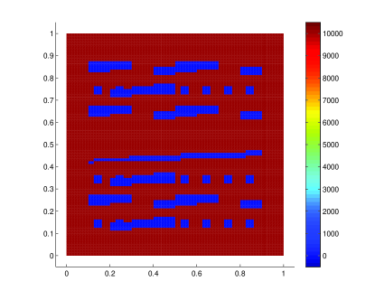
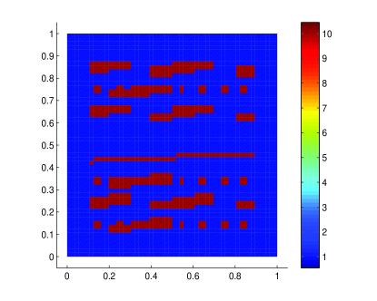
Refer to caption
(a) κ1subscript𝜅1\kappa_{1}
Refer to caption
(b) κ2subscript𝜅2\kappa_{2}
Figure 7.3: High-contrast fields in the numerical experiments.

7.1 Numerical results for reduced mixed GMsFE basis methods

In this subsection, we consider the elliptic equation in mixed formulation (1.1), where the coefficient function k(x,μ)𝑘𝑥𝜇k(x,\mu) is defined by

k(x,μ)=1000010sin(20μ+x1x2)+(cos(μ)+1.2)κ1+25,𝑘𝑥𝜇100001020𝜇subscript𝑥1subscript𝑥2𝜇1.2subscript𝜅125k(x,\mu)=\frac{10000}{10\sin(20\mu+x_{1}x_{2})+\big{(}\cos(\mu)+1.2\big{)}\kappa_{1}+25},

where κ1subscript𝜅1\kappa_{1} is a high-contrast field and depicted in Figure 7.3 (left), and the source function f(x,μ)𝑓𝑥𝜇f(x,\mu) is

f(x,μ)=(x20.5)cos(π(x10.5)).𝑓𝑥𝜇subscript𝑥20.5𝜋subscript𝑥10.5f(x,\mu)=(x_{2}-0.5)\cos\big{(}\pi(x_{1}-0.5)\big{)}.

Here x:=(x1,x2)Dassign𝑥subscript𝑥1subscript𝑥2𝐷x:=(x_{1},x_{2})\in D and the random parameter μU(1,1)similar-to𝜇𝑈11\mu\sim U(-1,1). The diffusion coefficient k(x,μ)𝑘𝑥𝜇k(x,\mu) is oscillating with respect to the random parameter μ𝜇\mu and highly heterogeneous with respect to the spatial variable x𝑥x. We apply EIM for k1(x,μ)superscript𝑘1𝑥𝜇k^{-1}(x,\mu) to achieve offline-online computation decomposition. For the discretization of the spatial domain, we use 80×80808080\times 80 uniform fine grid, where the reference solution is computed by the mixed FEM with the lowest Raviart-Thomas FE space. The mixed GMsFEM is implemented on the 8×8888\times 8 coarse grid. We choose |Ξtrain|=200subscriptΞtrain200|\Xi_{\text{train}}|=200 parameter values, and select |Ξop|=10subscriptΞ𝑜𝑝10|\Xi_{op}|=10 optimal samples from the training set ΞtrainsubscriptΞtrain\Xi_{\text{train}} by the greedy algorithm (Algorithm 4). The mixed GMsFEM is used to compute the snapshots, we take li(μ)=5subscript𝑙𝑖𝜇5l_{i}(\mu)=5 for each coarse block ωisubscript𝜔𝑖\omega_{i} and each μΞop𝜇subscriptΞ𝑜𝑝\mu\in\Xi_{op}, thus the number of the snapshot is nsnapi=j=1ntli(μj)=50superscriptsubscript𝑛snap𝑖superscriptsubscript𝑗1subscript𝑛𝑡subscript𝑙𝑖subscript𝜇𝑗50n_{\text{snap}}^{i}=\sum_{j=1}^{n_{t}}l_{i}(\mu_{j})=50 for each coarse block ωisubscript𝜔𝑖\omega_{i}. To show the efficacy of greedy algorithm for selecting the optimal sample set ΞopsubscriptΞ𝑜𝑝\Xi_{op}, we use two methods to select ΞopsubscriptΞ𝑜𝑝\Xi_{op}: the greedy algorithm and random selection, and then compare the results. For the numerical example, we consider the four different reduced GMsFE basis methods: reduced mixed GMsFE basis method using greedy algorithm and BOCV (RmGMsB-GBOCV), reduced mixed GMsFE basis method using greedy algorithm and POD (RmGMsB-GPOD), reduced mixed GMsFE basis method using random selection and BOCV (RmGMsB-RBOCV), and reduced mixed GMsFE basis method using random selection and POD (RmGMsB-RPOD). The first two methods use the greedy algorithm to select ΞopsubscriptΞ𝑜𝑝\Xi_{op}, while the last two methods are performed by randomly choosing 101010 parameter samples from ΞtrainsubscriptΞtrain\Xi_{\text{train}}.

To compare the approximation accuracy of the four reduced mixed GMsFE basis methods, we randomly choose 100010001000 samples from the parameter space and compute the average of relative error defined in (7.45) and (7.46) for the four methods. In Figure 7.4, we depict average relative velocity error versus number of local basis functions for the four reduced mixed GMsFE basis methods. By the figure we have three observations: (1) as the number of local basis functions increases, the approximation becomes more accurate for all methods; (2) RmGMsB-GBOCV method always achieves better approximation than RmGMsB-RBOCV, and RmGMsB-GPOD gives better approximation than RmGMsB-RPOD when the number of local GMsFE basis functions is more than 333; (3) BOCV approach renders better accuracy than POD approach. To visualize the individual errors of the first 100100100 samples, we plot the relative errors for the four methods in Figure 7.5, which shows that: (1) the error of RmGMsB-GBOCV is much less sensitive to the parameter samples compared with RmGMsB-RBOCV, and the POD approaches have the same situation; (2) BOCV approaches generally gives better approximation than POD approaches. Figure 7.6 shows the velocity solution profile of the example for the three methods: mixed FEM on fine grid (reference solution), RmGMsB-GBOCV and RmGMsB-GPOD. The figure shows all the velocity profiles have very good agreement and the reduced mixed GMsFE basis methods provide accurate approximation to the original fine scale model.
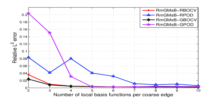
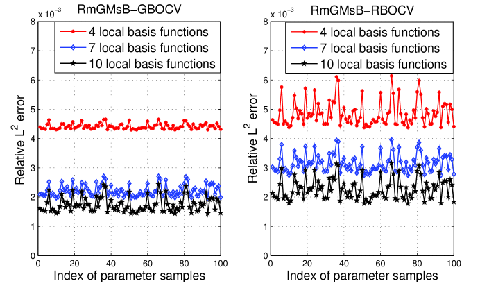
Refer to caption
Figure 7.4: The average relative error for velocity versus number of local basis functions for RmGMsB-GBOCV, RmGMsB-GPOD, RmGMsB-RBOCV and RmGMsB-RPOD, 80×80808080\times 80 fine grid, and 8×8888\times 8 coarse grid.
Refer to caption
Refer to caption
Figure 7.5: The relative error for 100100100 samples by RmGMsB-GBOCV, RmGMsB-GPOD, RmGMsB-RBOCV and RmGMsB-RPOD, 80×80808080\times 80 fine grid, and 8×8888\times 8 coarse grid.
Refer to caption
Figure 7.6: The mean of velocity profile, 555 local GMsFE basis functions on each coarse edge, the first row are the velocity in x-axis direction and the second row are the velocity in y-axis direction.

7.2 Numerical results for reduced model’s representation method

In this section, we consider two examples to illustrate the performance of reduced model representation using LSMOS and STAOMP. In the first example, we use a multivariate function to highlight the differences between LSMOS and STAOMP. For the second example, we consider an elliptic PDE with multi-dimensional parameters and apply LSMOS and STAOMP to obtain a reduced model representation for solution.

7.2.1 Numerical example I: a multivariate function

Let us consider the function

u(x,μ):=i=12xiμi+sin(π4(x1+13i=13μi))+cos(π4(x2+13i=46μi)),assign𝑢𝑥𝜇superscriptsubscript𝑖12subscript𝑥𝑖subscript𝜇𝑖𝜋4subscript𝑥113superscriptsubscriptproduct𝑖13subscript𝜇𝑖𝜋4subscript𝑥213superscriptsubscriptproduct𝑖46subscript𝜇𝑖u(x,\mu):=\sum_{i=1}^{2}x_{i}\mu_{i}+\sin\big{(}\frac{\pi}{4}(x_{1}+\frac{1}{3}\prod_{i=1}^{3}\mu_{i})\big{)}+\cos\big{(}\frac{\pi}{4}(x_{2}+\frac{1}{3}\prod_{i=4}^{6}\mu_{i})\big{)},

For the discretization of the spatial domain, we use 50×50505050\times 50 uniform grid and will consider the two variable-separation methods: LSMOS and STAOMP. With regard to LSMOS, we take εon=1.3×10³superscript𝜀on1.3superscript103\varepsilon^{\text{on}}=1.3\times 10^{-3} in Algorithm 5 and take 900900900 parameter samples for snapshots, the representation (3.12) can be obtained by Algorithm 5 with M=6𝑀6M=6. We use Legendre polynomials with degree up to Ng=5subscript𝑁𝑔5N_{g}=5 to approximate {ζi(μ)}i=1Msuperscriptsubscriptsubscript𝜁𝑖𝜇𝑖1𝑀\{\zeta_{i}(\mu)\}_{i=1}^{M} based on least square methods. Hence, the number of the total orthogonal polynomial basis is Mg=462subscript𝑀𝑔462M_{g}=462. For STAOMP, we take 160160160 parameter samples for snapshots, i.e., nt=160subscript𝑛𝑡160n_{t}=160, and construct 101010 optimal basis functions {vj(x)}j=16superscriptsubscriptsubscript𝑣𝑗𝑥𝑗16\{v_{j}(x)\}_{j=1}^{6} for spatial space, and set εon=1.3×10³superscript𝜀on1.3superscript103\varepsilon^{\text{on}}=1.3\times 10^{-3} in Algorithm 6, 160160160 parameter samples and 100100100 spatial coordinates are selected for snapshots, then we apply Algorithm 6 to construct the representation u(x,μ)i=1Mtc(I(i))ΨI(i)(μ,x)𝑢𝑥𝜇superscriptsubscript𝑖1MtcI𝑖subscriptΨI𝑖𝜇𝑥u(x,\mu)\approx\sum_{i=1}^{\text{Mt}}\textbf{c}(\emph{I}(i))\Psi_{\emph{I}(i)}(\mu,x) with Mt=41Mt41\text{Mt}=41. Based on these representations, we choose 100010001000 samples and compute the average relative error, which is defined as follows,

εu=1Ni=1Nu(x,μi)u~(x,μi)L2u(x,μi)L2,subscript𝜀𝑢1𝑁superscriptsubscript𝑖1𝑁subscriptnorm𝑢𝑥subscript𝜇𝑖~𝑢𝑥subscript𝜇𝑖superscript𝐿2subscriptnorm𝑢𝑥subscript𝜇𝑖superscript𝐿2\displaystyle\varepsilon_{u}=\frac{1}{N}\sum_{i=1}^{N}\frac{\|u(x,\mu_{i})-\tilde{u}(x,\mu_{i})\|_{L^{2}}}{\|u(x,\mu_{i})\|_{L^{2}}},

where N=1000𝑁1000N=1000 and u~(x,μi)~𝑢𝑥subscript𝜇𝑖\tilde{u}(x,\mu_{i}) is the solution by LSMOS or STAOMP. We list the average relative errors in Table 1 along with the average online CPU time. From the table, we find that: (1) for LSMOS, the approximation error decays fast when the number of terms increases; (2) using much fewer terms, STAOMP can achieve the same accuracy as LSMOS; (3) the magnitude of CPU time for STAOMP is much smaller than that of LSMOS.

Table 1: Comparison of relative mean errors ε𝜀\varepsilon and the average online CPU time for different approaches. Mt is the number of terms retained in reduced model representation.
  Strategies Mt εusubscript𝜀𝑢\varepsilon_{u} CPU time
LSMOS 1×46214621\times 462 1.10×1011.10superscript1011.10\times 10^{-1} 4.12×10⁴s4.12superscript104𝑠4.12\times 10^{-4}s
2×46224622\times 462 1.33×1021.33superscript1021.33\times 10^{-2} 7.80×10⁴s7.80superscript104𝑠7.80\times 10^{-4}s
3×46234623\times 462 1.87×1031.87superscript1031.87\times 10^{-3} 1.50×10³s1.50superscript103𝑠1.50\times 10^{-3}s
4×46244624\times 462 1.80×1031.80superscript1031.80\times 10^{-3} 2.10×10³s2.10superscript103𝑠2.10\times 10^{-3}s
5×46254625\times 462 1.70×1031.70superscript1031.70\times 10^{-3} 2.30×10³s2.30superscript103𝑠2.30\times 10^{-3}s
STAOMP 41 1.20×1031.20superscript1031.20\times 10^{-3} 9.86×10⁵s9.86superscript105𝑠9.86\times 10^{-5}s
 

7.2.2 Numerical example II: an elliptic PDE with multi-dimensional parameters

In this subsection, we consider the elliptic equation (1.1) with the source term

f(x)=(x1+1)cos(πx2),x(0,1)2.formulae-sequence𝑓𝑥subscript𝑥11𝜋subscript𝑥2𝑥superscript012f(x)=(x_{1}+1)\cos(\pi x_{2}),~{}~{}x\in(0,1)^{2}.

Let a(x,μ)𝑎𝑥𝜇a(x,\mu) be a random field, which is characterized by a two point exponential covariance function cov[a]covdelimited-[]𝑎\text{cov}[a], i.e.,

cov[a](x1,y1;x2,y2)=σ2exp(|x1x2|22lx2|y1y2|22ly2),covdelimited-[]𝑎subscript𝑥1subscript𝑦1subscript𝑥2subscript𝑦2superscript𝜎2superscriptsubscript𝑥1subscript𝑥222superscriptsubscript𝑙𝑥2superscriptsubscript𝑦1subscript𝑦222superscriptsubscript𝑙𝑦2\displaystyle\text{cov}[a](x_{1},y_{1};x_{2},y_{2})=\sigma^{2}\exp\bigg{(}-\frac{|x_{1}-x_{2}|^{2}}{2l_{x}^{2}}-\frac{|y_{1}-y_{2}|^{2}}{2l_{y}^{2}}\bigg{)}, (7.47)

where (xi,yi)subscript𝑥𝑖subscript𝑦𝑖(x_{i},y_{i}) (i=1,2𝑖12i=1,2) is the spatial coordinate in D𝐷D. Here the variance σ2=1superscript𝜎21\sigma^{2}=1, correlation length lx=ly=0.2subscript𝑙𝑥subscript𝑙𝑦0.2l_{x}=l_{y}=0.2. The random coefficient a(x,μ)𝑎𝑥𝜇a(x,\mu) is obtained by truncating a Karhunen-Loève expansion, i.e.,

a(x,μ):=E[a]+i=1Nγibi(x)μi,assign𝑎𝑥𝜇𝐸delimited-[]𝑎superscriptsubscript𝑖1𝑁subscript𝛾𝑖subscript𝑏𝑖𝑥subscript𝜇𝑖\displaystyle a(x,\mu):=E[a]+\sum_{i=1}^{N}\sqrt{\gamma_{i}}b_{i}(x)\mu_{i}, (7.48)

where E[a]=6𝐸delimited-[]𝑎6E[a]=6 and the random vector μ:=(μ1,μ2,,μN)Nassign𝜇subscript𝜇1subscript𝜇2subscript𝜇𝑁superscript𝑁\mu:=(\mu_{1},\mu_{2},...,\mu_{N})\in\mathbb{R}^{N}. Each μisubscript𝜇𝑖\mu_{i} (i=1,,N𝑖1𝑁i=1,\cdots,N) is uniformly distributed in the interval (1,1)11(-1,1). The diffusion coefficient k(x,μ)𝑘𝑥𝜇k(x,\mu) in (1.1) is defined as follows,

k(x,μ)=a(x,μ)khc,𝑘𝑥𝜇𝑎𝑥𝜇subscript𝑘𝑐k(x,\mu)=a(x,\mu)k_{hc},

where khc=104κ1subscript𝑘𝑐superscript104subscript𝜅1k_{hc}=\frac{10^{4}}{\kappa_{1}} and κ1subscript𝜅1\kappa_{1} is depicted in Figure 7.3 (left), a(x,μ)𝑎𝑥𝜇a(x,\mu) take the first thirteen terms of a(x,μ)𝑎𝑥𝜇a(x,\mu), i.e., N=12𝑁12N=12 in KLE (7.48). We note that k1superscript𝑘1k^{-1} is not affine with respect to the parameter μ𝜇\mu. Here we apply STAOMP to k1superscript𝑘1k^{-1} to get affine expression and achieve offline-online computation decomposition. The reference solutions are computed by the mixed FEM on 60×60606060\times 60 fine grid. We compute the mixed GMsFE basis on 10×10101010\times 10 coarse grid.

For the example, 500500500 parameter samples are selected for the training set ΞtrainsubscriptΞtrain\Xi_{\text{train}}. Then we use the greedy algorithm (Algorithm 4) to select |Ξop|=40subscriptΞ𝑜𝑝40|\Xi_{op}|=40 optimal samples from the training set ΞtrainsubscriptΞtrain\Xi_{\text{train}}, and take li(μ)=5subscript𝑙𝑖𝜇5l_{i}(\mu)=5 for each coarse block ωisubscript𝜔𝑖\omega_{i} and each μΞop𝜇subscriptΞ𝑜𝑝\mu\in\Xi_{op}, so the number of the snapshots is nsnapi=200superscriptsubscript𝑛snap𝑖200n_{\text{snap}}^{i}=200 for each coarse block ωisubscript𝜔𝑖\omega_{i}. Then we use RmGMsB-GBOCV to get the reduced multiscae basis and apply LSMOS and STAOMP to the reduced model representation. For LSMOS, we randomly choose 200020002000 parameter samples for the snapshots, which are computed by RmGMsB-GBOCV model with 777 local basis functions. For LSMOS, we take the first M𝑀M KLE terms in (3.12). Here we take M=3,4,5𝑀345M=3,4,5, respectively. They are corresponding to the third, forth and fifth row in Table 2. Then use Legendre polynomials with total degree up to Ng=4subscript𝑁𝑔4N_{g}=4 to approximate the KLE coefficients {ζi(μ)}i=1Msuperscriptsubscriptsubscript𝜁𝑖𝜇𝑖1𝑀\{\zeta_{i}(\mu)\}_{i=1}^{M}, and the total number of the Legendre polynomial basis functions is Mg=1820subscript𝑀𝑔1820M_{g}=1820. For STAOMP, we use POD to construct 666 optimal global basis functions for spatial space, and choose 707070 parameter samples and 100100100 spatial coordinates to get the reduced model representation by Algorithm 6, where the tolerance error εon=1×10⁴subscript𝜀on1superscript104\varepsilon_{\text{on}}=1\times 10^{-4} for both velocity and pressure. To assess the approximation by the model reduction methods, we randomly choose 100010001000 samples and compute the average relative errors defined as (7.45), (7.46). The results are listed in Table 2 along with the average online CPU time per sample. In the table, εv1superscriptsubscript𝜀𝑣1\varepsilon_{v}^{1} and εp1superscriptsubscript𝜀𝑝1\varepsilon_{p}^{1} are the relative errors based on the reference solutions computed by mixed FEM on fine grid, while εv2superscriptsubscript𝜀𝑣2\varepsilon_{v}^{2} and εp2superscriptsubscript𝜀𝑝2\varepsilon_{p}^{2} are the relative errors based on the reference solution computed by RmGMsB-GBOCV. From Table 2, we can see: (1) from the forth and sixth column of the table, we can see that the approximation by the three approaches is almost identical, which means that RmGMsB-GBOCV model can be accurately expressed by the reduced model representation using LSMOS or STAOMP; (2) the average CPU time per sample by STAOMP is the smallest among all of the approaches. The numerical example shows that the STAOMP method achieves a good trade-off in both approximation accuracy and computation efficiency. We note that the average online CPU time per sample is 21.444421.444421.4444 seconds using mixed FEM on fine grid. This time is much larger than the reduced model methods.

Table 2: Comparison of relative mean errors and the average online CPU time for different approaches. MtvsubscriptMt𝑣\text{Mt}_{v} is the number of terms of reduced model representation for velocity, and MtpsubscriptMt𝑝\text{Mt}_{p} is the number of terms of reduced model representation for pressure
  Strategies MtvsubscriptMt𝑣\text{Mt}_{v} MtpsubscriptMt𝑝\text{Mt}_{p} εv1superscriptsubscript𝜀𝑣1\varepsilon_{v}^{1} εv2superscriptsubscript𝜀𝑣2\varepsilon_{v}^{2} εp1superscriptsubscript𝜀𝑝1\varepsilon_{p}^{1} εp2superscriptsubscript𝜀𝑝2\varepsilon_{p}^{2} CPU time
RmGMsB 0.63×1020.63superscript1020.63\times 10^{-2} 2.76×1022.76superscript1022.76\times 10^{-2} 0.3841s0.3841𝑠0.3841s
LSMOS 5460 5460 0.64×1020.64superscript1020.64\times 10^{-2} 7.52×1057.52superscript1057.52\times 10^{-5} 2.77×1022.77superscript1022.77\times 10^{-2} 2.50×1032.50superscript1032.50\times 10^{-3} 1.02×10²s1.02superscript102𝑠1.02\times 10^{-2}s
7280 7280 0.63×1020.63superscript1020.63\times 10^{-2} 6.27×1066.27superscript1066.27\times 10^{-6} 2.76×1022.76superscript1022.76\times 10^{-2} 1.70×1031.70superscript1031.70\times 10^{-3} 1.68×10²s1.68superscript102𝑠1.68\times 10^{-2}s
9100 9100 0.63×1020.63superscript1020.63\times 10^{-2} 5.98×1075.98superscript1075.98\times 10^{-7} 2.76×1022.76superscript1022.76\times 10^{-2} 6.60×1046.60superscript1046.60\times 10^{-4} 1.84×10²s1.84superscript102𝑠1.84\times 10^{-2}s
STAOMP 36 40 0.63×1020.63superscript1020.63\times 10^{-2} 9.45×1069.45superscript1069.45\times 10^{-6} 2.76×1022.76superscript1022.76\times 10^{-2} 1.40×1031.40superscript1031.40\times 10^{-3} 2.02×10⁴s2.02superscript104𝑠2.02\times 10^{-4}s
 

7.3 Example of two-phase flow in random porous media

In this numerical example, we consider the following two-phase flow problem (in the absence of gravity and capillary effects) with zero Neumann boundary condition

{v=η(S)k(x,μ)pinD,v=qinD,St+(fw(S)v)=qsinD,casesformulae-sequence𝑣𝜂𝑆𝑘𝑥𝜇𝑝in𝐷formulae-sequence𝑣𝑞in𝐷𝑆𝑡subscript𝑓𝑤𝑆𝑣subscript𝑞𝑠in𝐷otherwise\displaystyle\begin{cases}\begin{split}&v=\eta(S)k(x,\mu)\nabla p~{}~{}\text{in}~{}~{}D,\\ &-\nabla\cdot v=q~{}~{}\text{in}~{}~{}D,\\ &\frac{\partial S}{\partial t}+\nabla\cdot\big{(}f_{w}(S)v\big{)}=q_{s}~{}~{}\text{in}~{}~{}D,\end{split}\end{cases} (7.49)

where the total mobility η(S)𝜂𝑆\eta(S) is defined by η(S)=S2/μw+(1S)2/μo𝜂𝑆superscript𝑆2subscript𝜇𝑤superscript1𝑆2subscript𝜇𝑜\eta(S)=S^{2}/\mu_{w}+(1-S)^{2}/\mu_{o} and v𝑣v refers to total velocity. Here μw/μo=0.1subscript𝜇𝑤subscript𝜇𝑜0.1\mu_{w}/\mu_{o}=0.1 is the ratio between viscosity of water and oil, the fractional flow function fw(S)subscript𝑓𝑤𝑆f_{w}(S) is given by

fw(S)=S2S2+μw/μo(1S)2,subscript𝑓𝑤𝑆superscript𝑆2superscript𝑆2subscript𝜇𝑤subscript𝜇𝑜superscript1𝑆2\displaystyle f_{w}(S)=\frac{S^{2}}{S^{2}+\mu_{w}/\mu_{o}(1-S)^{2}},

where S𝑆S is the saturation of water and q𝑞q is the source term for pressure equation and the source term for the saturation equation is expressed by

qs=max(q,0)+fw(S)min(q,0).subscript𝑞𝑠𝑞0subscript𝑓𝑤𝑆𝑞0q_{s}=\max(q,0)+f_{w}(S)\min(q,0).

We consider a logarithmic random field,

k(x,μ):=exp(κ2+a(x,μ)),assign𝑘𝑥𝜇subscript𝜅2𝑎𝑥𝜇k(x,\mu):=\exp\big{(}\kappa_{2}+a(x,\mu)\big{)},

where κ2subscript𝜅2\kappa_{2} is depicted in Figure 7.3 (right), and a(x,μ)𝑎𝑥𝜇a(x,\mu) is a stochastic field, which is characterized by a two point exponential covariance function cov[a]covdelimited-[]𝑎\text{cov}[a] in (7.47). Here the variance σ2=1superscript𝜎21\sigma^{2}=1, correlation length lx=ly=0.02subscript𝑙𝑥subscript𝑙𝑦0.02l_{x}=l_{y}=0.02. The random field a(x,μ)𝑎𝑥𝜇a(x,\mu) is obtained by truncating Karhunen-Loève expansion (7.48), where E[a]=0𝐸delimited-[]𝑎0E[a]=0 and the random vector μ:=(μ1,μ2,,μN)Nassign𝜇subscript𝜇1subscript𝜇2subscript𝜇𝑁superscript𝑁\mu:=(\mu_{1},\mu_{2},...,\mu_{N})\in\mathbb{R}^{N} and μiN(0,1)similar-tosubscript𝜇𝑖𝑁01\mu_{i}\sim N(0,1) (i=1,,N𝑖1𝑁i=1,\cdots,N), i.e, normal distribution with zero mean and unit variance. We truncate the KLE (7.48) after the first 202020 terms to represent the random field a(x,μ)𝑎𝑥𝜇a(x,\mu). To fulfil offline-online computation decomposition, we use EIM for k1(x,μ)superscript𝑘1𝑥𝜇k^{-1}(x,\mu) and get an affine expression.

The reference solution is computed on a 56×56565656\times 56 fine grid. The mixed GMsFEM is performed on a 7×7777\times 7 coarse grid. We solve the flow equation on the coarse grid using RmGMsB-GBOCV first and then reconstruct the fine-scale velocity field as a superposition of the GMsFE basis functions. The reconstructed velocity field is used to solve the saturation equation with a finite volume method on the fine grid. We use an Implicit Pressure Explicit Saturation (IMPES) formulation for the coupled system (7.49).

Let Sinsuperscriptsubscript𝑆𝑖𝑛S_{i}^{n} be the saturation at the ithsubscript𝑖𝑡i_{th} fine element Kihsuperscriptsubscript𝐾𝑖K_{i}^{h} at time tn=t0+nΔtsubscript𝑡𝑛subscript𝑡0𝑛Δ𝑡t_{n}=t_{0}+n\Delta t, where t0subscript𝑡0t_{0} is the initial time. Then the saturation equation can be discretized by

|Kih|Sin+1SinΔt+Kihfw(S^n)(vn)=|Kih|(qs)i,superscriptsubscript𝐾𝑖superscriptsubscript𝑆𝑖𝑛1superscriptsubscript𝑆𝑖𝑛Δ𝑡subscriptsuperscriptsubscript𝐾𝑖subscript𝑓𝑤superscript^𝑆𝑛𝑣𝑛superscriptsubscript𝐾𝑖subscriptsubscript𝑞𝑠𝑖|K_{i}^{h}|\frac{S_{i}^{n+1}-S_{i}^{n}}{\Delta t}+\int_{\partial K_{i}^{h}}f_{w}(\hat{S}^{n})(v\cdot n)=|K_{i}^{h}|(q_{s})_{i},

where (qs)isubscriptsubscript𝑞𝑠𝑖(q_{s})_{i} is the average value of qwsubscript𝑞𝑤q_{w} on Kihsuperscriptsubscript𝐾𝑖K_{i}^{h}, and S^nsuperscript^𝑆𝑛\hat{S}^{n} is the upwind flux. For numerical test, we take q𝑞q to be zero except for the top-left and bottom-right coarse-grid elements, where q𝑞q takes the values 1 and 11-1, respectively. This is a traditional two-spot problem, in which the water is injected at the top-left corner and oil is produced at the bottom-right corner. Moreover, we set the initial staturation to be zero.

For the pressure equation in (7.49), we construct the multiscale finite element space VHMC,CVsuperscriptsubscript𝑉𝐻subscript𝑀𝐶𝐶𝑉V_{H}^{M_{C},CV} by RmGMsB-GBOCV at initial time, and use it for all the time levels. We randomly choose nt=|Ξtrain|=200subscript𝑛𝑡subscriptΞtrain200n_{t}=|\Xi_{\text{train}}|=200 parameter samples and select |Ξop|=40subscriptΞ𝑜𝑝40|\Xi_{op}|=40 optimal samples by greedy algorithm to compute the snapshots. For each coarse block ωisubscript𝜔𝑖\omega_{i} and each μΞop𝜇subscriptΞ𝑜𝑝\mu\in\Xi_{op}, we take li(μ)=7subscript𝑙𝑖𝜇7l_{i}(\mu)=7 local basis functions to construct snapshots (nsnapi=j=1ntli(μj)=280superscriptsubscript𝑛snap𝑖superscriptsubscript𝑗1subscript𝑛𝑡subscript𝑙𝑖subscript𝜇𝑗280n_{\text{snap}}^{i}=\sum_{j=1}^{n_{t}}l_{i}(\mu_{j})=280 for each coarse block ωisubscript𝜔𝑖\omega_{i}) for the reduced GMsFE basis. Then we employ RmGMsB-GBOCV to simulate the flow equation and get the following weak formulation,

{a(vHN(μ),u;μ)b(u,pHN(μ);μ)=0uVHMC,CV,b(vHN(μ),q;μ)=l(q)qQH,|Kih|Sin+1SinΔt+Kihfw(S^n)(vn)=|Kih|(qs)i.casesformulae-sequence𝑎superscriptsubscript𝑣𝐻𝑁𝜇𝑢𝜇𝑏𝑢superscriptsubscript𝑝𝐻𝑁𝜇𝜇0for-all𝑢superscriptsubscript𝑉𝐻subscript𝑀𝐶𝐶𝑉𝑏superscriptsubscript𝑣𝐻𝑁𝜇𝑞𝜇𝑙𝑞for-all𝑞subscript𝑄𝐻superscriptsubscript𝐾𝑖superscriptsubscript𝑆𝑖𝑛1superscriptsubscript𝑆𝑖𝑛Δ𝑡subscriptsuperscriptsubscript𝐾𝑖subscript𝑓𝑤superscript^𝑆𝑛𝑣𝑛superscriptsubscript𝐾𝑖subscriptsubscript𝑞𝑠𝑖otherwise\displaystyle\begin{cases}\begin{split}&a(v_{H}^{N}(\mu),u;\mu)-b(u,p_{H}^{N}(\mu);\mu)=0~{}~{}~{}\forall~{}u\in V_{H}^{M_{C},CV},\\ &b(v_{H}^{N}(\mu),q;\mu)=l(q)~{}~{}~{}\forall~{}q\in Q_{H},\\ &|K_{i}^{h}|\frac{S_{i}^{n+1}-S_{i}^{n}}{\Delta t}+\int_{\partial K_{i}^{h}}f_{w}(\hat{S}^{n})(v\cdot n)=|K_{i}^{h}|(q_{s})_{i}.\end{split}\end{cases} (7.50)
Refer to caption
Refer to caption
Refer to caption
Refer to caption
Refer to caption
Refer to caption
Figure 7.7: The mean of water saturation profiles at t=600𝑡600t=600 (the first row) and t=1000𝑡1000t=1000 (the second row), 56×56565656\times 56 fine grid, and 7×7777\times 7 coarse grid, the number of local multiscale basis functions is 444.
Refer to caption
Refer to caption
Refer to caption
Refer to caption
Refer to caption
Refer to caption
Figure 7.8: The variance of water saturation profiles at t=600𝑡600t=600 (the first row) and t=1000𝑡1000t=1000 (the second row), 56×56565656\times 56 fine grid, 7×7777\times 7 coarse grid, the number of local multiscale basis functions is 444.
Table 3: Comparison of the average online CPU time for water saturation per sample at different time levels for the two approaches: STAOMP and RmGMsB-GBOCV, the number of local multiscale basis functions is 444.
  Strategies t=500𝑡500t=500 t=1000𝑡1000t=1000 t=1500𝑡1500t=1500 t=2000𝑡2000t=2000
STAOMP 1.60×10³s1.60superscript103𝑠1.60\times 10^{-3}s 1.50×10³s1.50superscript103𝑠1.50\times 10^{-3}s 1.40×10³s1.40superscript103𝑠1.40\times 10^{-3}s 1.50×10³s1.50superscript103𝑠1.50\times 10^{-3}s
RmGMsB-GBOCV 1.78371.78371.7837 5.02275.02275.0227 6.63406.63406.6340 7.83117.83117.8311
 

Water saturation is an important quantity for the model. We utilize STAOMP to represent the water saturation S(x,t,μ)𝑆𝑥𝑡𝜇S(x,t,\mu) of the reduced model (7.50). To this end, we choose the set of parameter samples Ξt={μi}i=1600subscriptΞ𝑡superscriptsubscriptsubscript𝜇𝑖𝑖1600\Xi_{t}=\{\mu_{i}\}_{i=1}^{600} and apply POD to the snapshots associated with ΞtsubscriptΞ𝑡\Xi_{t} and get the optimal global basis functions {Si^(x,t)}i=14superscriptsubscript^subscript𝑆𝑖𝑥𝑡𝑖14\{\hat{S_{i}}(x,t)\}_{i=1}^{4}. To approximate random parameter space, we use Hermite polynomial basis functions with total degree up to Ng=3subscript𝑁𝑔3N_{g}=3 and denote the basis set by {pi(μ)}i=11771superscriptsubscriptsubscript𝑝𝑖𝜇𝑖11771\{p_{i}(\mu)\}_{i=1}^{1771}. A finite dimensional approximation space for {S(x,t,μi);μiΓ}𝑆𝑥𝑡subscript𝜇𝑖subscript𝜇𝑖Γ\{S(x,t,\mu_{i});\mu_{i}\in\Gamma\} is then obtained by

S4×1771:=span{pi(μ)Sj^(x,t):1i1771,1j4}.assignsubscriptS41771spanconditional-setsubscript𝑝𝑖𝜇^subscript𝑆𝑗𝑥𝑡formulae-sequence1𝑖17711𝑗4\textbf{S}_{4\times 1771}:=\text{span}\{p_{i}(\mu)\hat{S_{j}}(x,t):1\leq i\leq 1771,1\leq j\leq 4\}.

To get a model reduction representation using STAOPM, we randomly choose 600600600 parameter samples, 646464 spatial points and 18 time levels for snapshots, and then use Algorithm 6 to construct a sparse representation S(x,t,μ)i=1Mtc(I(i))ΨI(i)(x,t,μ)𝑆𝑥𝑡𝜇superscriptsubscript𝑖1MtcI𝑖subscriptΨI𝑖𝑥𝑡𝜇S(x,t,\mu)\approx\sum_{i=1}^{\text{Mt}}\textbf{c}(\emph{I}(i))\Psi_{\emph{I}(i)}(x,t,\mu), where Mt=160Mt160\text{Mt}=160, I={1,,1771}×{1,,4}𝐼1177114I=\{1,\cdots,1771\}\times\{1,\cdots,4\} and Ψi(t,μ)=pi1(μ)Si2^(x,t)subscriptΨ𝑖𝑡𝜇subscript𝑝subscript𝑖1𝜇^subscript𝑆subscript𝑖2𝑥𝑡\Psi_{i}(t,\mu)=p_{i_{1}}(\mu)\hat{S_{i_{2}}}(x,t).

To calculate the approximation errors by RmGMsB-GBOCV and STAOPM, we randomly choose 100010001000 samples and compute the RmGMsB-GBOCV model (7.50) and evaluate the reduced model representation by STAOMP for each sample. The relative mean errors for saturation S𝑆S is defined by

εs(t)=1Ni=1NS(x,t,μi)SH(x,t,μi)L1(D)S(x,t,μi)L1(D),subscript𝜀𝑠𝑡1𝑁superscriptsubscript𝑖1𝑁subscriptnorm𝑆𝑥𝑡subscript𝜇𝑖subscript𝑆𝐻𝑥𝑡subscript𝜇𝑖superscript𝐿1𝐷subscriptnorm𝑆𝑥𝑡subscript𝜇𝑖superscript𝐿1𝐷\displaystyle\varepsilon_{s}(t)=\frac{1}{N}\sum_{i=1}^{N}\frac{\|S(x,t,\mu_{i})-S_{H}(x,t,\mu_{i})\|_{L^{1}(D)}}{\|S(x,t,\mu_{i})\|_{L^{1}(D)}}, (7.51)

where N=1000𝑁1000N=1000, S(x,t,μi)𝑆𝑥𝑡subscript𝜇𝑖S(x,t,\mu_{i}) is the solution of fine scale model, and SH(x,t,μi)subscript𝑆𝐻𝑥𝑡subscript𝜇𝑖S_{H}(x,t,\mu_{i}) is the solution of (7.50) by RmGMsB-GBOCV or STAOPM.
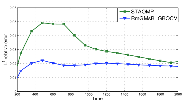
Refer to caption
Figure 7.9: The average relative error for water saturation versus different time levels. the number of local multiscale basis functions is 444.

Figure 7.7 shows the mean of water saturations at t=600𝑡600t=600 and t=1000𝑡1000t=1000 for the different methods. Here the reference solution is computed by mixed FEM on fine grid. By the figure, we see that the model reduction methods provide accurate approximation to the reference saturation in the average sense. Figure 7.8 demonstrates the variance of water saturation at t=600𝑡600t=600 and t=1000𝑡1000t=1000 for the different methods. By the figure, we can find: (1) the largest variance occurs along the advancing water front; (2) there is no clear difference for the variance profiles between the reference solution and RmGMsB-GBOCV solution; (3) compared with reference solution, the STAOMP approach renders some clear difference for the variance approximation around the water front. Table 3 lists the average online CPU time per sample for the water saturation by the different approaches. We find that the STAOMP method significantly improves computation efficiency especially for the later time levels. Moreover, the online CPU time of STAOMP method is almost independent of the time level. This is an important advantage of the STAOMP method for two-phase flow simulation. Figure 7.9 shows the average relative error for water saturation defined by (7.51) versus different time levels for the different methods. By the figure, we find that the error by STAOMP decays after the water break-through time and then tends to be stable.
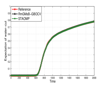
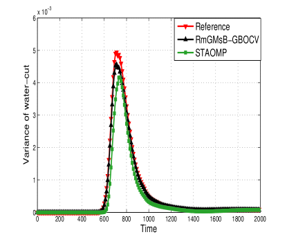
Refer to caption
Refer to caption
Figure 7.10: The expectation (left) and variance (right) of water-cut curves

Water-cut is also an important quantity for the water-oil two-phase flow. The water-cut is defined as the fraction of water in the produced fluid and is given by qw/qtsubscript𝑞𝑤subscript𝑞𝑡q_{w}/q_{t}, where qt=qo+qwsubscript𝑞𝑡subscript𝑞𝑜subscript𝑞𝑤q_{t}=q_{o}+q_{w}, with qosubscript𝑞𝑜q_{o} and qwsubscript𝑞𝑤q_{w} being the flow rates of oil and water at the production edge of the model. In particular, qw=Doutfw(S)vn𝑑ssubscript𝑞𝑤subscriptsuperscript𝐷𝑜𝑢𝑡subscript𝑓𝑤𝑆𝑣𝑛differential-d𝑠q_{w}=\int_{\partial D^{out}}f_{w}(S){v}\cdot{n}ds, qt=Ωoutvn𝑑ssubscript𝑞𝑡subscriptsuperscriptΩ𝑜𝑢𝑡𝑣𝑛differential-d𝑠q_{t}=\int_{\partial\Omega^{out}}{v}\cdot{n}ds, where Doutsuperscript𝐷𝑜𝑢𝑡{\partial D^{out}} is the out-flow boundary.

For the water-cut, we utilize STAOMP to approximate the water-cut of the reduced model (7.50). We use the set of parameter samples Ξt={μi}i=1600subscriptΞ𝑡superscriptsubscriptsubscript𝜇𝑖𝑖1600\Xi_{t}=\{\mu_{i}\}_{i=1}^{600} and apply POD to the snapshots associated with ΞtsubscriptΞ𝑡\Xi_{t} to obtain 666 optimal global basis functions {wi^(t)}i=16superscriptsubscript^subscript𝑤𝑖𝑡𝑖16\{\hat{w_{i}}(t)\}_{i=1}^{6}. We use the same polynomial basis functions as the water saturation, and get a finite dimensional approximation space

W6×1771:=span{pi(μ)wj^(t):1i1771,1j6}.assignsubscriptW61771spanconditional-setsubscript𝑝𝑖𝜇^subscript𝑤𝑗𝑡formulae-sequence1𝑖17711𝑗6\textbf{W}_{6\times 1771}:=\text{span}\big{\{}p_{i}(\mu)\hat{w_{j}}(t):1\leq i\leq 1771,1\leq j\leq 6\big{\}}.

To get a model reduction representation using STAOPM, we randomly choose 600600600 parameter samples and 101010 time levels for snapshots, and then use Algorithm 6 to construct a sparse representation W(t,μ)i=1Mtc(I(i))ΨI(i)(t,μ)𝑊𝑡𝜇superscriptsubscript𝑖1MtcI𝑖subscriptΨI𝑖𝑡𝜇W(t,\mu)\approx\sum_{i=1}^{\text{Mt}}\textbf{c}(\emph{I}(i))\Psi_{\emph{I}(i)}(t,\mu) with Mt=195Mt195\text{Mt}=195, where I={1,,1771}×{1,,6}𝐼1177116I=\{1,\cdots,1771\}\times\{1,\cdots,6\} and Ψi(t,μ)=pi1(μ)wi2^(t)subscriptΨ𝑖𝑡𝜇subscript𝑝subscript𝑖1𝜇^subscript𝑤subscript𝑖2𝑡\Psi_{i}(t,\mu)=p_{i_{1}}(\mu)\hat{w_{i_{2}}}(t).

Figure 7.10 shows the expectation (left) and variance (right) of the water-cut curves with the different approaches. The figure shows that the expectation curves of the water-cut are all nearly identical. This implies a good mean approximation for water-cut using RmGMsB-GBOCV and STAOMP; The variance of water-cut rises rapidly at the break-through time, and then decays fast after a while. The error of water-cut variance by STAOMP is slightly larger around the water break-through time than other time instances.

8 Conclusions

In the paper, we presented two variable-separation representations for random fields: LSMOS and STAOMP. The LSMOS is devoted to constructing a KL expansion and building a relation between the random inputs and the stochastic basis functions based on least-squares methods. The STAOMP provides a tensor product for the random field and achieves a sparse approximation by using orthogonal-matching-pursuit method. The two methods can be applied to get a variable-separation approximation for any generic functions with random inputs. For the multiscale problems with high-dimensional random inputs, the computation would be prohibitive if we directly solve the problems for a many-query situation. To overcome the difficulty, we developed reduced mixed GMsFE basis methods to improve the computation efficiency. To this end, we have chosen a few optimal parameters from the parameter space by a greedy algorithm. Then we use the optimization methods BOCV and POD to obtain reduced multiscale basis functions and get a reduced order model. In the reduced multiscale basis methods, the whole computation admits offline-online decomposition. In the online phase, a reduced model is solved for each parameter sample. Although the offline computation may be expensive, the online computation is efficient. We have carefully compared the performance of the different reduced mixed GMsFE basis methods, and found that BOCV may lead to the reduced model with better accuracy and robustness than POD does. The dimension of the space spanned by the set of reduced multiscale basis functions is much smaller than the dimension of the original full order model, but it depends on the size of coarse grid. When the size of coarse grid is large, the computation of the reduced order model may be still expensive. To further improve the efficiency of the online computation, we construct a sparse representation for model’s outputs by combining the reduced mixed GMsFE basis methods and STAOMP. This is very desirable for predicting the model’s outputs for arbitrary parameter values and quantifying the uncertainty propagation. We applied the proposed reduced mixed GMsFE basis methods and the model’s sparse representation method to a few numerical models with multiscale and random inputs. Careful numerical analysis is carried out for these computational models.

Although the proposed methods significantly reduces the online computation, it takes much effort in offline computation stage. In future, we will explore novel methods to substantially decrease the offline computation burden as well.

Acknowledgments

We would like to thank the helpful discussion with Prof. Yalchin Efendiev for the work. We acknowledge the support of Chinese NSF 11471107.

References

  • [1] J. Aarnes, Y.  Efendiev and L.  Jiang, Mixed multiscale finite element methods using limited global information, Multiscale Modeling and Simulation, 7 (2008),  pp. 655–676.
  • [2] G. Allaire and R. Brizzi, A multiscale finite element method for numerical homogennization, Multiscale Modelling and Simulation, 4 (2005), pp. 790-812.
  • [3] T. Arbogast, G. Pencheva, M.F. Wheeler, and I. Yotov, A multiscale mortar mixed finite element method, Multiscale Modelling and Simulation, 6 (2007), pp. 319-346.
  • [4] G. Beylkin and M. Mohlenkamp, Algorithms for numerical analysis in high dimensions, SIAM Journal on Scientific Computing, 26 (2005), pp. 2133–2159.
  • [5] A. Buffa, Y. Maday, A. Patera, C. Prudhomme, and G. Turinici, A priori convergence of the greedy algorithm for the parametrized reduced basis method, ESAIM: Mathematical Modelling and Numerical Analysis, 46 (2012), pp. 595–603.
  • [6] Y. Chen, J.S. Hesthaven, Y. Maday, and J. Rodríguez, Certified reduced basis methods and output bounds for the harmonic Maxwell’s equations, SIAM Journal on Scientific Computing, 32 (2010), pp. 970–996.
  • [7] Z. Chen and T. Hou, A mixed multiscale finite element method for elliptic problems with oscillating coefficients, Mathematics of Computation, 72 (2003), pp. 541–576.
  • [8] M. Chevreuil, R. Lebrun, A. Nouy, and P. Rai, A least-squares method for sparse low rank approximation of multivariate functions, SIAM/ASA Journal on Uncertainty Quantification, 3 (2015), pp. 897–921.
  • [9] F. Chinesta, P. Ladeveze, and E. Cueto, A short review on model order reduction based on proper generalized decomposition, Arch. Comput. Methods Eng, 18 (2011), pp. 395–404.
  • [10] E. Chung, Y. Efendiev, and C. Lee, Mixed generalized multiscale finite element methods and applications, Multiscale Modelling and Simulation, 13 (2015), pp. 338–366.
  • [11] A. Doostan and G. Iaccarino, A least-squares approximation of partial differential equations with high-dimensional random inputs, J. Comput. Phys, 228 (2009), pp. 4332–4345.
  • [12] A. Doostan, G. Iaccarino, and N. Etemadi, A least-squares approximation of high-dimensional uncertain systems, Annual Research Briefs, Center for Turbulence Research, Stanford University, (2007), pp. 121–132.
  • [13] P. Dostert, Y. Efendiev, and T. Hou, Multiscale finite element methods for stochastic porous media flow equations and application to uncertainty quantification, Comput. Methods Appl. Mech. Engrg. 197 (2008), pp. 3445-3455.
  • [14] W. E and B. Engquist, The heterogeneous multi-scale methods, Comm. Math. Sci., 1 (2003), pp. 87–133.
  • [15] Y. Efendiev, J. Galvis, and T.Y. Hou, Generalized multiscale finite element methods (gmsfem), J. Comput. Phys, 251 (2013), pp. 116–135.
  • [16] Y. Efendiev and T. Hou, Multiscale finite element methods: Theory and Applications, Springer Science and Business Media, 2009.
  • [17] J. Eftang, M. Grepl, and A. Patera, A posteriori error bounds for the empirical interpolation method, Comptes Rendus Mathematique, 348 (2010), pp. 575-579.
  • [18] M. Elad, Sparse and redundant representations: from theory to applications in signal and image processing, Springer, 2009.
  • [19] A. L. Gerner and K. Veroy, Certified reduced basis methods for parametrized saddle point problems, SIAM Journal on Scientific Computing, 34 (2012), pp. A2812–A2836.
  • [20] D. González, A. Ammar, F. Chinesta, and E. Cueto, Recent advances on the use of separated representations, Int. J. Numer. Meth. Engng, 81 (2010), pp. 637–661.
  • [21] R. Handler, K. Housiadas, and A. Beris, Karhunen–loeve representations of turbulent channel flows using the method of snapshots, International journal for numerical methods in fluids, 52 (2006), pp. 1339–1360.
  • [22] T. Hughes, G. Feijoo, L. Mazzei, and J. Quincy, The variational multiscale method - a paradigm for computational mechanics, Comput. Methods Appl. Mech. Engrg, 166 (1998), pp. 3–24.
  • [23] D. Huynh, G. Rozza, S. Sen, and A. Patera, A successive constraint linear optimization method for lower bounds of parametric coercivity and inf-sup stability constants, Comptes Rendus Mathematique, 345 (2007), pp. 473-478.
  • [24] L. Jiang, I. Mishev, and Y. Li, Stochastic mixed multiscale finite element methods and their applications in random porous media, Comput. Methods Appl. Mech. Engrg. 199 (2010), pp. 2721-2741.
  • [25] L. Jiang and Q. Li, Reduced multiscale finite element basis methods for elliptic pdes with parameterized inputs, Journal of Computational and Applied Mathematics, 301 (2016), pp. 101–120.
  • [26] L. Jiang and M. Presho, A resourceful splitting technique with applications to deterministic and stochastic multiscale finite element methods, Multiscale Modelling and Simulation, 10 (2012), pp. 954-985.
  • [27] M. Loeve, Probability theory, Graduate texts in mathematics, 46 (1978), pp. 0–387.
  • [28] N. Nguyen, A multiscale reduced-basis method for parametrized elliptic partial differential equations with multiple scales, J. Comput. Phys. 227 (2008), pp. 9807-9822.
  • [29] A. Quarteroni, G. Rozza, and A. Manzoni, Certified reduced basis approximation for parametrized partial differential equations and applications, Journal of Mathematics in Industry, 1 (2011), pp. 1–49.
  • [30] G. Rozza, D. Huynh, and A. Patera, Reduced basis approximation and a posteriori error estimation for affinely parametrized elliptic coercive partial differential equations, Arch Comput Methods Eng. 15 (2008), pp. 229-275.
  • [31] I. Rish, and G. Grabarnik, Sparse modeling: theory, algorithms, and applications, CRC Press, 2014.
  • [32] W. Schilders, H. van der Vorst, and J. Rommes, Model Order Reduction: Theory, Research Aspects and Applications, Springer, 2008.
  • [33] J. Tropp and A. Gilbert, Signal recovery from random measurements via orthogonal matching pursuit, Information Theory, IEEE Transactions on. 53 (2007), pp. 4655–4666.