The Power of Principled Bayesian Methods in the Study of Stellar Evolution

Abstract

It takes years of effort employing the best telescopes and instruments to obtain high-quality stellar photometry, astrometry, and spectroscopy. Stellar evolution models contain the experience of lifetimes of theoretical calculations and testing. Yet most astronomers fit these valuable models to these precious datasets by eye. We show that a principled Bayesian approach to fitting models to stellar data yields substantially more information over a range of stellar astrophysics. We highlight advances in determining the ages of star clusters, mass ratios of binary stars, limitations in the accuracy of stellar models, post-main-sequence mass loss, and the ages of individual white dwarfs. We also outline a number of unsolved problems that would benefit from principled Bayesian analyses.

1 Introduction

1.1 Motivation

Collecting good stellar photometry and spectroscopy is expensive. For deep photometry or spectroscopy we use some of the largest ground-based telescopes, which cost approximately $1/s to build and operate. For many globular cluster studies, we use the Hubble Space Telesope, which is even more precious. Likewise, stellar models are expensive. Careers have been devoted to understanding stellar structure and evolution and capturing that knowledge in stellar codes and isochrones. Yet, typically when astronomers compare their precious stellar data to these valuable models, they do so by overplotting theory and data in the same color-magnitude diagrams (CMDs), then adjusting various parameters until the theory and data appear to fit best, as judged by eye. This so called chi-by-eye procedure is neither strictly reproducible nor does it yield the highest quality results because the human eye cannot optimize multidimensional parameters or visualize multidimensional data, each datum of which has its own uncertainties. Fortunately, there are new statistical solutions available.

In the following sections, we present our Bayesian statistical approach to this data-fitting problem, and show through a series of examples how this approach is substantially more capable than the classical, chi-by-eye approach. We also outline a number of unsolved problems that would benefit from Bayesian analysis and point the interested reader toward our open-source software.

1.2 Methodological Limitations to Obtaining Scientific Objectives

When investigators are faced with rich datasets, such as photometry, spectroscopy, and proper motions or radial velocities, they tend to take a step-by-step approach to analyzing their data by breaking the problem down into smaller pieces with different teams working on different apsects of the problem. For instance, one team may analyze the spectroscopy to determine the cluster metallicity, though that in turn depends on the effective temperature for the stars in question, for which they may return to the literature for values. Another team may isolate a sample of stars with a certain cut-off probability of being cluster members based on radial velocity and/or proper motions, then publish CMDs along with chi-by-eye based isochrone fits. Yet, how are stars to be weighted in these isochrone fits? Shouldn’t every star have a weight inversely proportional to its photometric errors and directly proportional to its probability of being a cluster member, at least above some threshold where the cluster membership probabilities blend into the larger pool of field stars? Historically it is often the case that yet another team performes a more detailed follow-up study by using the previously-determined metallicity and cluster membership probabilities to perform a more thorough isochrone fit, perhaps varying modeling parameters such as convective overshoot or mixing length, though still fitting models to data by eye. Yet, such a study may derive a reddening value for the cluster that is different from the one assumed by the group deriving cluster spectroscopic metallicity, which ultimately depended on stellar effective temperature and therefore also on reddening. Without the spectroscopic material in hand, this study cannot solve for all of the important parameters simultaneously.

This step-by-step approach can be inconsistnent, relying on different assumed cluster parameters (most typically, distance and reddening) and different underlying stellar evolution models. This approach also assumes that errors can be propagated by the simple rules of independent normal errors. Yet stellar evolution is inherently non-linear (e.g., stellar lifetimes and luminosities are not linearly dependent on stellar masses), so there is no a priori reason to expect that error distributions are normal.

Besides the general issue of objectivity, there are other limitations in comparing models to data by eye. One is that stellar isochrones do not generally match stars throughout the CMD, and this mismatch can be filter dependent. This is clearly visible in the CMDs of NGC 188 presented by Sarajedini et al. (1999, figure 10), where, for instance, a given set of isochrones matches best around 6 Gyr for a $U-B$ vs. $V$ CMD, but appears older than 7 Gyrs in $B-V$ vs. $V$ and $V-I$ vs. $V$ CMDs. Additionally, in all of the CMDs presented by Sarajedini et al., the isochrones are a few tenths of a magnitude too blue along the red giant branch (RGB). How does one properly judge a match between theory and observations by eye when some parts of the theory may match better than others? While we do not have a complete answer to this question, we believe that the first step in this direction is to develop an objective technique and demonstrate how it performs. A better approach would be to supplement the observational errors with model errors that captured the uncertainty in stellar evolution models. This will be difficult to incorporate until theorists are able to quantify the uncertainties in their models.

Another question regarding model errors has to do with the proper adjustment of tunable parameters within a model, e.g., mixing length, and how best to match them to cluster data. If one does this fit by eye, it is infeasible to allow all the other parameters to vary; one usually starts by performing a differential comparison with some best fit. Yet this is probably sensitive to the starting point, , to whatever the author thinks is the nominal best fit, and a chi-by-eye fit necessarily focuses on just a few features in one or maybe two CMDs rathar than simultaneously fitting all the available photometry. The problem is compounded if one wants to generalize this and vary more than one theory ingredient at a time. For example, theory ingredients may be coupled or may match the data in some correlated fashion.

Standard methods also do not allow one to take advantage of ancillary information such as cluster distances from trigonometric parallaxes or the moving cluster method, binary mass ratios from radial velocity monitoring, or white dwarf (WD) masses from fitting the Balmer lines, etc. Our Bayesian method allows such ancillary information to be incorporated into an analysis in a principled manner.

Our technical goal is to avoid as many of these pitfalls as possible and fully use valuable data. This means analyzing a star cluster with all the data we can bring to bear and to consider these data simultaneously via an objective and rigorous technique. This technical goal is in service of our scientific goals, which are 1) to improve our understanding of stellar evolution by more accurately and precisely comparing models to data, and 2) deriving better stellar cluster and field star ages. In Section 2 we introduce Bayesian statistics, which form the foundation of our statistical approach. In Section 3 we introduce our Bayesian software. In Section 4 we illustrate its application with the dual hope of convincing current users of chi-by-eye to start using more rigorous approaches and to spark interest in the development of new imaginative statistical approaches to the myriad rich datasets that are now available to astronomers.

2 Bayesian Basics

2.1 Introduction

Thomas Bayes (1702-1761) was a British mathematician and Presbyterian minister, known for having formulated a special case of Bayes’ theorem, which was published posthumously (Wikipedia, retrieved Jan 12, 2014). Subsequently, Pierre-Simon Laplace (1749-1827) introduced a general version of the theorem and used it to approach problems in celestial mechanics, medical statistics, reliability, and jurisprudence.

2.2 Bayesian Inference

Bayes’ theorem states that

$$p(\hbox{model}|\hbox{data})=\frac{p(\hbox{data}|\hbox{model})\ p(\hbox{model})}{p(\hbox{data})}$$ (1)

where $p(\hbox{model}|\hbox{data})$ is the joint (multivariate) probability density function of a set of model parameters given the data, $p(\hbox{data}|\hbox{model})$ is the likelihood function, and $p(\hbox{model})$ is the prior distribution of the model parameters. The prior distribution folds in knowledge from previous analyses of other datasets, knowledge that one has before considering the current dataset. In contrast, the posterior distribution, $p(\hbox{model}|\hbox{data})$, summarizes the combined knowledge for the model parameters stemming both from the current data and from prior information. The likelihood function describes the statistical model for the current data set. The value for $p(\hbox{data})$ is obtained by integrating the numerator over the possible values of the model parameters so that

$$p(\hbox{model}|\hbox{data})=\frac{p(\hbox{data}|\hbox{model})\ p(\hbox{model})}{\int p(\hbox{data}|\hbox{model})\ p(\hbox{model})\ d\hbox{model}}.$$ (2)

This integral is a normalizing constant that ensures that the posterior distribution properly integrates to one. In practice, we use numerical techniques such as Markov chain Monte Carlo that do not require us to compute the integral.

3 BASE-9

3.1 Introduction

We have developed a Bayesian approach to fitting isochrones to stellar photometry (see [von Hippel et al. (2006)]; [DeGennaro et al. (2009)]; [van Dyk et al. (2009)]; [Stein et al. (2013)]). Our Bayesian approach is implemented in the software package called BASE-9 for Bayesian Analysis of Stellar Evolution with 9 Parameters. BASE-9 compares main sequence through asymptotic giant branch stellar evolution models ([Girardi et al. (2000)]; [Yi et al. (2001)]; [Dotter et al. (2008)]) as well as WD interior ([Wood (1992)]; [Montgomery et al. (1999)]; [Renedo et al. (2010)]) and atmosphere models ([Bergeron, Wesemael, & Beauchamp (1995)]) to photometry in any combination of photometric bands for which there are data and models. BASE-9 was designed to analyze star clusters and accounts for individual errors for each data point; includes ancillary information such as cluster membership probabilities from proper motions or radial velocities, cluster distance (e.g., from Hipparcos parallaxes or the moving cluster method), and cluster metallicity from spectroscopic studies; and can incorporate information such as individual stellar mass estimates from dynamical studies of binaries or spectroscopic atmospheric analyses of WDs. BASE-9 uses a computational technique known as Markov chain Monte Carlo (MCMC) to derive the Bayesian joint posterior distribution given in Equation 1 for six parameter categories (cluster age, metallicity, helium content, distance, and reddening, and optionally a parameterized IFMR, see [Stein et al. (2013)]) and brute-force numerical integration for three parameter categories (stellar mass, binarity, and cluster membership). The last three of these parameter categories include one parameter per star whereas the first six parameter categories refer to the entire cluster. As a result, for star clusters BASE-9 actually fits hundreds or thousands of parameters (= 3 N_star + 6) simultaneously.

3.2 Mathematics Behind BASE-9

The details of the statistical methods we use are described more completely in [Stein et al. (2013)], see also [DeGennaro et al. (2009)] and [van Dyk et al. (2009)]. In specifying the likelihood function, we use stellar evolution models to predict observed photometric magnitudes as a function of the several cluster and stellar parameters, $\mbox{\boldmath{$\Theta$}}=$ ($m-M$, [Fe/H], log(age), $A_{\rm V}$, stellar mass, etc.). These predictions incorporate main-sequence/red-giant models, white dwarf models, a parameterized initial-final mass relationship, and the possibility of unresolved binary stars. Specifically, letting $\mbox{\boldmath{$\mu$}}_{i}(\mbox{\boldmath{$\Theta$}})$ be the predicted photometric magnitudes for star $i$, the likelihood function is

$$\small L(\mbox{\boldmath{$\Theta$}},\mbox{\boldmath{$Z$}}|\mbox{\boldmath{$X$}},\mbox{\boldmath{$\Sigma$}})=\prod_{i=1}^{n}\Bigg{[}{Z_{i}\over\sqrt{(2\pi)^{n}|\mbox{\boldmath{$\Sigma$}}_{i}|}}\exp\left(-{1\over 2}\Big{(}\mbox{\boldmath{$X$}}_{i}-\mbox{\boldmath{$\mu$}}_{i}(\mbox{\boldmath{$\Theta$}})\Big{)}^{\top}\mbox{\boldmath{$\Sigma$}}_{i}^{-1}\Big{(}\mbox{\boldmath{$X$}}_{i}-\mbox{\boldmath{$\mu$}}_{i}(\mbox{\boldmath{$\Theta$}})\Big{)}\right)$$

$$\small\qquad\qquad+\ \ (1-Z_{i})p_{\rm field}(\mbox{\boldmath{$X$}}_{i})\Bigg{]},$$ (3)

where $n$ is the number of stars in the dataset, $\mbox{\boldmath{$X$}}=(\mbox{\boldmath{$X$}}_{1},\ldots,\mbox{\boldmath{$X$}}_{n})$ are the observed photometric magnitudes, $\mbox{\boldmath{$\Sigma$}}=(\mbox{\boldmath{$\Sigma$}}_{1},\ldots,\mbox{\boldmath{$\Sigma$}}_{n})$ are the known variance-covariance matrices of the observed magnitudes, $\mbox{\boldmath{$Z$}}=(Z_{1},\ldots,Z_{n})$ are unknown zero-one variables that indicate whether each star is a cluster star $(Z_{i}=1)$ or a field star $(Z_{i}=0)$, and $p_{\rm field}$ is the distribution of photometric magnitudes for field stars and is assumed uniform in the range of the data.

Treating the denominator of Equation 1 as a normalizing constant, the posterior distribution in our Bayesian analysis can be written, namely

$$p(\mbox{\boldmath{$\Theta$}},\mbox{\boldmath{$Z$}}|\mbox{\boldmath{$X$}},\mbox{\boldmath{$\Sigma$}})\propto L(\mbox{\boldmath{$\Theta$}}|\mbox{\boldmath{$X$}},\mbox{\boldmath{$\Sigma$}})p(\mbox{\boldmath{$\Theta$}},\mbox{\boldmath{$Z$}}),$$ (4)

where $p(\mbox{\boldmath{$\Theta$}},\mbox{\boldmath{$Z$}})$ is the prior distribution for the stellar parameters and of the cluster-member indicator variables. Computationally, BASE-9 works on the marginal posterior distribution of Equation 3.2 obtained by summing over $Z$ and numerically integrating over the star-specific masses.

The prior distribution quantifies the knowledge and uncertainty we have about the stellar parameters before considering the current data set. The posterior distribution combines this information with that in the current data, updating our knowledge about the stellar parameters in light of the new information.

4 Applications

4.1 Cluster Properties from Main Sequence Turn-off Stars and White Dwarfs

The age for the halo of the Milky Way is derived from main sequence turn-off (MSTO) fitting of globular clusters, whereas the age of the disk of the Milky Way is derived from white dwarf models fit to the white dwarf luminosity function. Because both of these age determinations are based on different and largely unrelated physics, we need to confirm whether they are on the same absolute age scale. The best way to accomplish this is to study single-age star clusters and derive both their MSTO ages and their WD cooling ages. Yet, to take full advantage of this approach, one must take great care to derive MSTO and WD ages consistently.

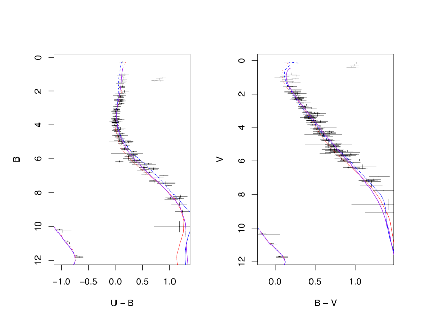
Figure 1: Isochrones for three different main-sequence model sets at the nominal age, distance, and metallicity of the Hyades. Solid purple lines represent the [Girardi et al. (2000)] models, dotted red lines represent the [Yi et al. (2001)] models, and dashed blue lines represent the [Dotter et al. (2008)] models. Gray points show additional Hyades photometry not used in these fits. (Figure from [DeGennaro et al. (2009)].)

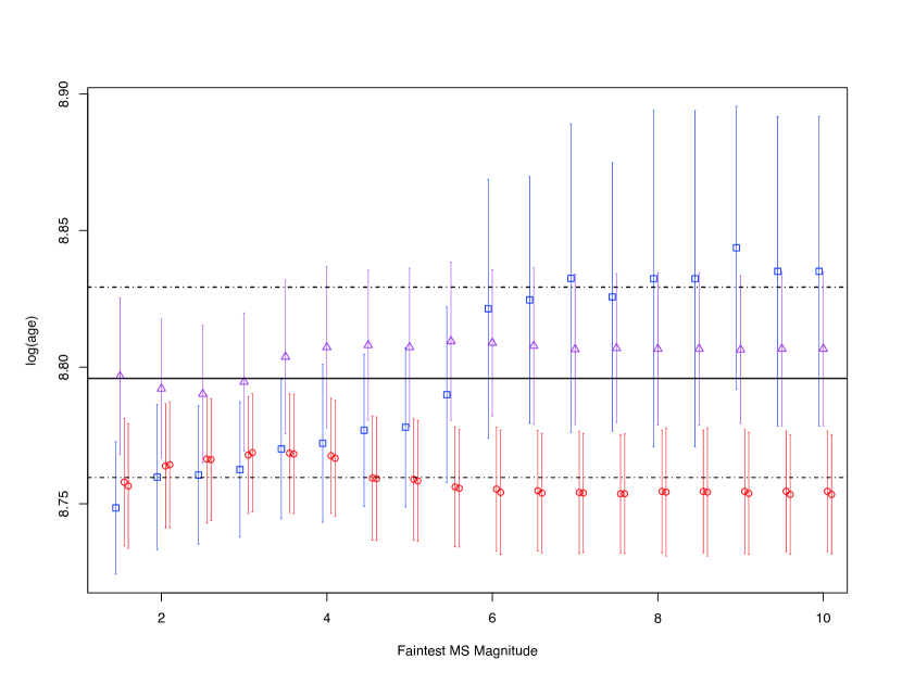
Figure 2: Derived log10(age) for the Hyades as a function of the faintest main sequence star included in the analysis. (Figure from [DeGennaro et al. (2009)].)

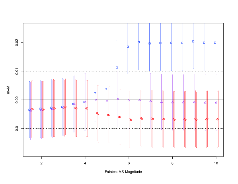
Figure 3: Derived Hyades distance modulus relative to [Perryman et al. (1998)] as a function of the faintest main sequence star included in the analysis. (Figure from [DeGennaro et al. (2009)].)

Figure 1, from [DeGennaro et al. (2009)], displays Hyades $UB$ and $BV$ CMDs along with overplotted isochrones from [Girardi et al. (2000)], [Yi et al. (2001)], and [Dotter et al. (2008)]. These isochrones represent fits that simultaneously incorporate the cluster main sequence and WDs. These fits do not include the MSTO or red giant branch (plotted in gray), as the goal of this particular study was to derive the cluster WD age. Yet, it is clear from this figure that each of these stellar evolution models fails to fit the lower main sequence, with different offsets for each model. None of these three sets of models claims to fit low mass stars, yet how does this mis-fitting propagate into creating a best fit isochrone? [DeGennaro et al. (2009)] circumvent this problem by studying the best fit as a function of depth along the main sequence, with more stars being included further down the main sequence in each of a succession of fits.

In Figure 2 we present the derived log10(age) for the Hyades as a function of the faintest main sequence star included in the analysis from [DeGennaro et al. (2009)]. The blue squares represent [Dotter et al. (2008)] models, the red circles represent two different runs of the [Yi et al. (2001)] models (to test sensitivity to starting values), and the purple triangles represent the [Girardi et al. (2000)] models. The error bars on the symbols span the 68% probability interval in the log10(age) posterior distribution. The horizontal lines are the mean and $\pm 1\sigma$ deviations of the most reliable estimate for the age of the Hyades as determined by MSTO fitting by [Perryman et al. (1998)]. In Figure 3 we present the offset in the derived distance modulus for the Hyades as a function of the faintest main sequence star included in the analysis of [DeGennaro et al. (2009)] relative to that found by [Perryman et al. (1998)]. The symbols have the same meaning as in Figure 2. The distance values comes from [Perryman et al. (1998)] and represents the prior information used in the analysis. We can see that in both figures most fits agree with previous values for the Hyades until $V\approx 8$, where we see larger departures. In the case of the Hyades, the most relevant constraint from prior work is the Hipparcos distance published by [Perryman et al. (1998)], and we can see the offset is well within the very small errors.

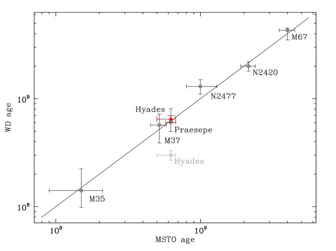
Figure 4: WD versus MSTO age for seven clusters. (Figure from [Jeffery (2009)].)

[Jeffery (2009)] continues this study and finds that the MSTO and WD ages are consistent to the limit of their study at 4 Gyr. Figure 4 shows the WD versus MSTO age for seven clusters from [Jeffery (2009)]. The age derived from the WDs in the Hyades by [DeGennaro et al. (2009)] using our Bayesian approach brings the Hyades age into agreement with the MSTO age for the first time (red solid triangle). The solid line shows the one-to-one correspondence between the WD and MSTO ages, and the gray point shows the most reliable WD age of the Hyades prior to the work by [DeGennaro et al. (2009)].

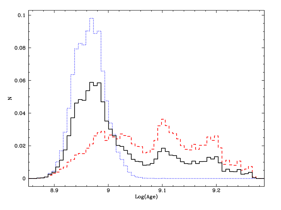
Figure 5: The age distribution of NGC 2360 with and without the inclusion of one particular WD. (Figure from [Jeffery (2009)].)

Perhaps more demonstrative of the power of the Bayesian approach is Figure 5 from [Jeffery et al. (2011)], which shows the shapes of age posterior distributions and their sensitivities to individual stars. The solid black line is the complete age posterior distribution when all WD candidates in NGC 2360 are included. The dotted blue line is the age distribution when WD5 is included as a cluster member. The red dashed line is the distribution when WD5 is excluded as a field star. This indicates the importance of this star in determining the location of the WD cooling sequence and hence measuring the cluster age.

4.2 Cluster Binary Stars

Figure 6 presents the simulated effects of unresolved binaries on the CMD. The black line is an isochrone from the [Yi et al. (2001)] models, which indicates the position of single stars. The complex hooks emanating from the isochrone show the effect of adding secondary stars to primary stars at specific points along the isochrone. The binary pairs closest to the main sequence isochrone have a secondary star with a mass of 0.4 $M_{\odot}$ and each successive point further away from the main sequence is the result of a higher mass secondary star until the final point 0.75 mag above the isochrone, where the binary consists of two equal mass stars. Figure 7 presents an enlargement of the area in Figure 6 around the three proximal binary sequences, including also an example photometric data point (in red) with errors. The photometry can match a number of different primary and secondary stars.

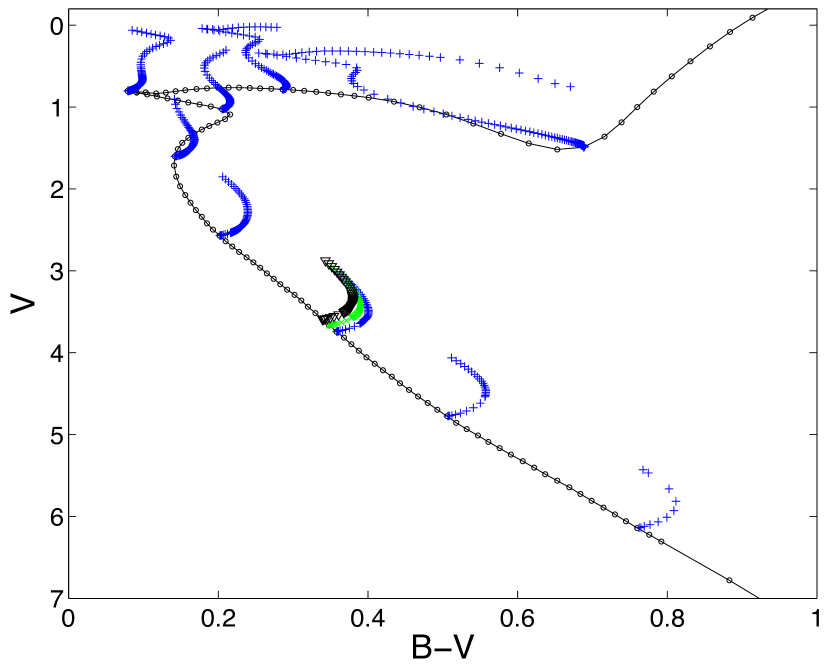
Figure 6: An example of the effects of unresolved binaries on the CMD.

Figure 7: Enlargement of the area around the three proximal binary sequences, including also an example photometric data point (in red) with errors.

Figure 8, an updated version from [van Dyk et al. (2009)], resents the joint posterior distribution for the primary and secondary masses of the star vB022 in the Hyades. The scatter plot shows the Monte Carlo sample from the posterior distribution using the three stellar evolution models discussed above and presented in Figures 1-3. The star has a posterior probability of cluster membership equal to 99.955% and the plot gives the conditional posterior distribution of the two masses given that the binary system is a member of the cluster. This is compared with a kinematic estimate of the two masses based on fitting radial velocities to this elicpsing double-lined spectroscopic binary and is indicated by the point with $\pm$ 1$\sigma$ error bars. The primary mass is marginally inconsistent ($\sim$2$\sigma$) and slightly lower ($\sim$ 0.02 to 0.03 $M_{\odot}$) than the more reliable external estimate. (All masses are in units of $M_{\odot}$.) These types of comparisons can provide tests of stellar evolution models.

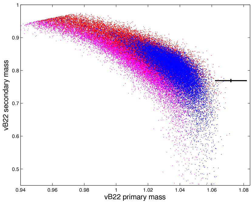
Figure 8: The joint posterior distribution for the primary and secondary masses of the Hyades binary vB022. (Figure from [van Dyk et al. (2009)].)

4.3 Sensitivity Analysis: Results Depend on Filters

[Hills et al. (2014)] showed that the cluster parameters one derives can depend on the filters one choses. This both demonstrates limitations in the stellar evolution models and is a cautionary tale to anyone who might compare cluster ages (or other parameters) fit from different filter photometry. Figure 9 shows CMDs for NGC 188 after the cluster was cleaned of most binaries. The overplotted isochrone is a fit based on [Yi et al. (2001)] models applied to $UBVRI$ photometry. The point types correspond to the assigned cluster membership probability for each star (filled circles have membership probabilities greater than 0.9, open circles indicate between 0.7 and 0.9 probability, open squares show probabilities less than 0.7). These probabilities result from the arithmetic mean of membership probabilities from [Stetson, McClure, & VandenBerg (2004)] (based on proper motions) and [Geller et al. (2008)] (based on radial velocities).

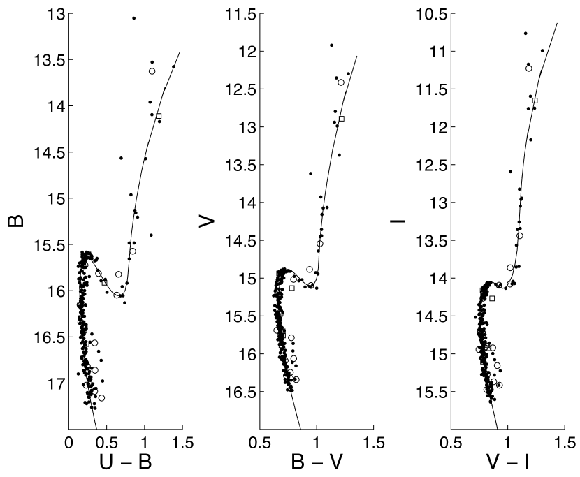
Figure 9: CMDs for NGC 188 in a range of optical bands. (Figure from [Hills et al. (2014)].)

Figure 10: Box-and-whisker plots for age across eight photometric band combinations based on [Yi et al. (2001)] models. (Figure from [Hills et al. (2014)].)

Figure 10 shows box-and-whisker plots from [Hills et al. (2014)] of age fits across eight photometric band combinations based on [Yi et al. (2001)] models. The box-and-whisker plots are a compact way of showing the degree to which a distribution is non-Gaussian. The central line indicates the median of the distribution and the upper and lower box edges indicate the 25th and 75th percentiles. The whiskers extend out to the most extreme non-outliers, and outliers are plotted individually. A data point is considered an outlier if it is smaller than $q_{1}-\frac{3}{2}(q_{3}-q_{1})$ or greater than $q_{3}+\frac{3}{2}(q_{3}-q_{1})$, where $q_{1}$ and $q_{3}$ are the 25th and 75th percentiles, respectively. Some filter combinations yield meaningfully different results, and many of these are inconsistent at the equivalent of 3$\sigma$.

4.4 Initial Final Mass Relation

Mass lost by stars ascending the red giant branch is poorly understood (see [Catelan 2009]). At the same time, red giant mass loss is key to interpreting globular cluster and old open cluster CMDs because it drives the morphology of the horizontal branch (HB). In more distant systems, such as M31, HB morphology may be our only clue to the ages of stellar systems. Yet this clue is fraught with uncertainty because we lack a properly determined mass loss formula for stellar models. A proper understanding of mass loss becomes even more important beyond the Local Group where we interpret stellar populations only through their integrated light.

Work to date has focused either on theoretical (e.g., [Blocker 1995]) or semi-empirical (e.g., [Reimers 1975]; [Judge & Stencel 1991]) parameterizations of this process or on constraints from the remnant WD masses (e.g., [Weidemann (2000)]; [Williams, Bolte, & Koester (2004)]; [Kalirai et al. (2005)]). Yet these approaches have been necessarily piecemeal, with either a focused examination of the theoretical constraints (e.g., [Vassiliadis & Wood 1993]) or an iterative and not self-consistent approach to deriving the mass lost from the mains sequence to the WDs (see [Salaris et al. (2009)] for a thorough critical evaluation). In addition, these mass loss studies are based on only a few key star clusters (e.g., [Origlia et al. 2007]) because quality data have been so limited.

An independent way to measure mass loss during the late stages of stellar evolution is to determine, via cluster ages, the mapping of initial zero age main sequence (ZAMS) masses to final WD masses, which is the so-called Initial-Final Mass Relation (IFMR). With the exception of Omega Cen and a few other globular clusters, star clusters are essentially or at least approximately single-age systems. As such, the age derived from the WDs should be equal to the age derived from the MSTO stars. The former incorporates the age of the WD precursor, the IFMR itself, and then WD cooling rates. Such work has been done in the past (e.g., [Weidemann (2000)]; [Kalirai et al. (2005)]; Williams, Bolte, & Koester (2004); Williams, Bolte, & Koester (2009)), though always in the context of a step-wise solution, often in an internally inconsistent manner ([Salaris et al. (2009)]). Because stellar evolution is a highly non-linear process, the step-wise approach does not adequately propagate errors, even when done consistently, and it certainly does not recover the entire posterior distribution on any parameterization of the IFMR. Within the Bayesian context, one can solve this problem with complete internal consistency for each stellar evolution model and recover the IFMR parameter distribution. In Figure 11 we show this type of analysis performed by [Stein et al. (2013)]. In this example, [Stein et al. (2013)] set the IFMR to be a simple linear model with two free parameters (its slope and intercept) and then used BASE-9 to fit and assess uncertainty in these two IFMR parameters while simultaneously fitting all the other cluster and stellar parameters. While the IFMR is unlikely to be linear, any given cluster constrains just a small mass range of this relation, and a linear fit is appropriate within this small range. [Stein et al. (2013)] also performed fits using broken-linear and quadratic IFMRs.

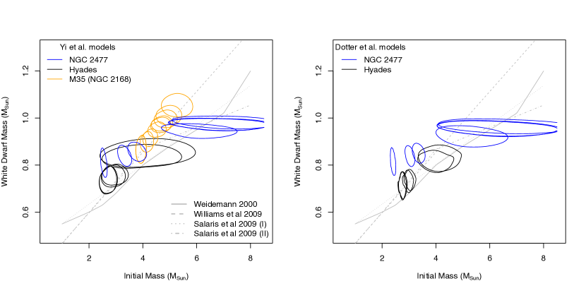
Figure 11: The initial and WD masses for WDs from the open clusters NGC 2477, the Hyades, and M35 analyzed using the [Yi et al. (2001)] models. Contours are 95% highest posterior density regions of each WD’s joint initial and final mass posterior distribution. In this particular analysis, the IFMR model enforces linearity within each cluster, but not between clusters. (Figure from [Stein et al. (2013)].)

4.5 Ages for Individual Field White Dwarfs

While one cannot typically derive ages for individual main sequence or red giant branch stars, one can derive ages for individual WDs because WDs have a mass-radius relation that constrains their luminosity. In many cases, this constraint is sufficient to yield useful ages. (In a few years, we expect GAIA astrometric results to open up new possibilities for determining the ages of individual stars.)

[Bergeron, Leggett, & Ruiz (2001)] improved the technique for deriving individual WD ages by comparing WD masses and $T_{\rm eff}$ values with WD cooling models. This technique relies on measuring $T_{\rm eff}$ from photometry or spectroscopy and log(g) from spectroscopy or WD surface area from trigonometric parallax. Because WDs have a mass-radius relation ([Hamada & Salpeter]), either log(g) or surface area yield mass, and the mass and $T_{\rm eff}$, when compared to a WD cooling model, yield the WD cooling age. The WD mass is relied upon again to infer its precursor mass through the imprecisely-known IFMR. The precursor mass is then converted to a pre-WD lifetime via stellar evolution models. Finally, the precursor lifetime is added to the WD cooling age to determine the total age of the WD.

The above-mentioned technique has its advantages and disadvantages. The foremost advantage is that it yields reasonably precise ages for individual WDs. Secondarily, for cool WDs with masses $\geq$ 0.7 M_⊙, the progenitor lifetime is short relative to the WD cooling age, and therefore uncertainties in the IFMR are unimportant (see, for instance, [von Hippel et al. (2006)], fig 16). On the negative side, this age technique involves many steps, some of which are often performed inconsistently. An additional negative is that one has to correctly propagate errors through many steps. Some errors may start out symmetrically distributed (e.g., $T_{\rm eff}$), but the assumptions behind the standard propagation of errors are not met (see [O’Malley, von Hippel, & van Dyk (2013)]), casting doubt on the estimates and errors that this approach produces.

Figure 12: Posterior probability projections in the age, distance, ZAMS mass planes for the WD J0003$-$0111 for each of four IFMRs and the [Montgomery et al. (1999)] WD cooling models. These IFMRs, from left to right, are the [Williams, Bolte, & Koester (2009)], [Weidemann (2000)], and [Salaris et al. (2009)] Linear and Piecewise relations. (Figure from [O’Malley, von Hippel, & van Dyk (2013)].)

Figure 12 displays the posterior distributions for a single representative WD (J0003$-$0111), fit with the [Montgomery et al. (1999)] WD models and each of four IFMRs studied by [O’Malley, von Hippel, & van Dyk (2013)]. There are detailed similarities in all four cases, and in fact the contours for all IFMRs peak near 6 Gyrs and 65 pc, yet the distributions are subtly different from one IFMR to another. [O’Malley, von Hippel, & van Dyk (2013)] showed such comparisons for 28 WDs and were able to make a detailed study of the effect of different IFMRs on implied WD ages.

4.6 Future Applications

In addition to the subjects studied above, there are a number of other problems in stellar astrophysics that we believe would benefit from a principled Bayesian analysis. A short list of examples follow.

4.6.1 Multiple populations in globular clusters

While it has been known for decades that some globular clusters contain stars with a range of abundances, it has only recently become clear that globular clusters can host multiple stellar populations. Exquisite Hubble Space Telescope photometry now clearly shows multiple main sequences, subgiant branches, or red giant branches in a number of clusters. This newly recognized complexity challenges current chi-by-eye approachs far more than past work on globular clusters, both because more parameters are involved in any fit and because newly abundant spectroscopic data tags individual stars with additional information indicating which population they likely belong to and some details about the properties of that population.

4.6.2 Carbon-to-oxygen ratio in WDs

Stellar evolution models predict the carbon-to-oxygen ratio as a function of stellar mass but these calculations are affected by uncertainties in the nuclear reaction rates, overshooting, and mass loss. Thus, it is important to check these results empirically both as a test of stellar evolution models and because the carbon-to-oxygen ratio affects the WD cooling rate, and thereby the implied age of any observed WD. The density-temperature phase diagram for carbon+oxygen mixtures has not been empirically verified at these densities and temperatures and thus crystallization and the possibility of phase separation of C and O remain as possible uncertainties in deriving ages for the oldest WDs, particularly those in globular clusters. One can use Bayesian techniques to compare families of WD models to the two or three globular clusters and eight open clusters with sufficient WD populations and perform simultaneous age fits for both the WDs and MSTO stars, with the carbon-to-oxygen ratio as a free parameter.

4.6.3 Width of the main sequence

What is the intrinsic width of the main sequence once one accounts for photometric errors, binaries, and other known effects? These other effects include rapid stellar rotation (e.g., [Mermilliod, Mayor, & Udry (2009)]; [James et al. (2010)]) and stellar activity (e.g., [Pace (2010)]), both of which are prevalent in young clusters. In some clusters, differential reddening broadens the main sequence (e.g., NGC 2477, [von Hippel, Gilmore & Jones (1995)]). For clusters where these effects can be minimized or properly modeled, a careful Bayesian analysis has the sensitivity to test for internal metallicity dispersions as small as $\sigma$([Fe/H]) = 0.02.

There are two reasons to perform this test. The first is to measure or place new limits on the degree of gas heterogeneity in the parent clouds that formed today’s open clusters and globular clusters. This in turn would measure the ratio of the turbulent mixing time scale to the length of time the cloud existed before forming stars. Such a metallicity heterogeneity would cause a broadening of the main sequence largely independent of stellar mass.

The second reason to perform this measurement is to test whether there are detectable signatures from the ingestion of planetary material during giant planet migration. This latter effect should be noticeable for stars with shallow convection zones such as F stars. [Pinsonneault, DePoy, & Coffee (2001)] find that stars hotter than $T_{\rm eff}$ = 6700 would have metallicities elevated by 0.02 dex after ingesting only one earth mass of iron. [Trilling, Lunine, & Benz (2002)] argue that it is likely that more planets are accreted onto their host star than remain in orbit, and thus if 10% of all solar type stars have planets we might expect an even greater fraction to have ingested planetary material. Unlike parent cloud heterogeneity, this effect would be mass dependent and thus we could distinguish the two possible sources. Measuring stellar photospheric abundance variations within a cluster could provide insight into the ubiquity and ultimate fate of planetary migration.

4.6.4 Tests of physical ingredients of stellar evolution

Convective core overshoot is a crucial ingredient in stellar models of stars with masses greater than about 1 solar mass, hence ages less than a few Gyr. In general, overshoot mixing applies to all stellar models with convective boundaries but the most dramatic evidence for this is in the convective core where overshoot mixing draws H-rich material into the core, thereby extending the main sequence lifetime of the star.

Hydrodynamic simulations of convection have been performed for a number of environments (e.g., [Freytag, Ludwig, & Steffen 1996]; [Meakin & Arnett 2007]) with the end result that it is possible to incorporate the improved understanding of overshoot mixing gained from these simulations into stellar evolution codes. This treatment of convective overshoot has been investigated in detail in models of AGB stars ([Herwig et al. 1997]; [Herwig 2000]) but has not been systematically applied to the CMD morphology of young and intermediate age open clusters. Current cluster photometry, combined with a principled Bayesian approach, can test whether or not the hydrodynamically-motivated overshoot mixing prescription is able to reproduce the CMD morphologies of various open clusters with a range of age and metallicity.

4.6.5 Coupling age information from multiple field WDs

Following on the results of [O’Malley, von Hippel, & van Dyk (2013)], it would be particularly useful if we could extract Galactic population age information from disk, thick disk, and halo populations of WDs. In many cases, we will have probabilistic population asignments based on proper motions and distances, yet there are other constraints such as a common IFMR, at least for a given metallicity, and different metallicity distributions for the precursor populations. These constraints, combined with the observational data, need to be combined in a simultaneous fit to recover the age distribution of our Galaxy’s major components.

5 Conclusions

We have used a number of examples to show that a principled Bayesian approach to fitting stellar data with models yields substantially more information with substantially higher precision than the classic chi-by-eye approach. We have demonstrated that our Bayesian technique yields more precise and accurate star clusters properties, mass ratios of binary stars, and ages of individual white dwarfs. We have further demonstrated that our technique illuminates limitations in the accuracy of stellar isochrones and quantifies post-main-sequence mass loss. There are a wide number of additional topics in stellar evolution that will benefit from principled Bayesian analysis.