Chebychev interpolations of the Gamma and Polygamma Functions and their analytical properties

in  memoriam
Cornelius Lanczos[6] 1893-1974 

address:
Email: KD.Reinartz@T-Online.de
Kieferndorfer Weg 30, D-91315 Höchstadt, GERMANY

keywords:
Gamma function, Sterling formula, Bernoulli numbers, Chebychev approximations, Chebyshev polynomials, Shifted Chebyshev polynomials, Invers Gamma function, Psi (Digamma) function, Harmonic function, Polygamma functions, Summation/Differentiation/Multiplication of Chebyshev approximations.

1 Introduction

The Gamma Function derived by Leonhard Euler (1729) is the generalization of discrete factorials:

$$z!=\Gamma\left(z+1\right)=\int_{0}^{\infty}\!{t}^{z-1}{e}^{-t}{dt},\quad\Re z>0$$ (1)

The numerical evaluation is not easy. Whittaker+Watson [10] and Temme [9] give a good discussion of the $\Gamma$ Function and several basic properties.
In contrast to that Lanczos [5] developed approximations with a restricted precision by using Chebyshev polynomials in the range [-1..+1] (instead of shifted polynomials which will be used exclusively in this paper). Chebychev polynomials were introduced into numerical analysis especially by Lanczos [6]in the US since 1935 and by Clenshaw [3] in GB since 1960.–

The next formula is due to James Stirling (1730)

$$\ln\Gamma\left(z\right)\,\sim\,ln\left(\sqrt{2\pi}\,{z}^{z-\frac{1}{2}}\,{{\rm e}^{-z}}\right)+\sum_{n=1}^{\infty}{\frac{B_{{2\,n}}}{2\,n\left(2\,n-1\right){z}^{2\,n-1}}}$$ (2)

The $B_{{2\,n}}$ are the Bernoulli numbers with a poor behaviour:

$$\begin{split}&\frac{1}{6},\,-\frac{1}{30},\,\frac{1}{42},\,-\frac{1}{30},\,\frac{5}{66},\,\frac{691}{2730},\,\frac{7}{6},\,-\frac{3617}{510},\,\frac{43867}{798},\,-\frac{174611}{330},\,\frac{854513}{138},-\frac{236364091}{2730},\\ &\quad\frac{8553103}{6},\,-\frac{23749461029}{870},\,\frac{8615841276005}{14322},\,\frac{7709321041217}{510},\,\frac{2577687858367}{6},...\end{split}$$ (3)

They decrease at the beginning only slowly and then grow with (2n)!. The complete terms in the infinite sum eq. 2 depend on n and z and grow nevertheless, especially if z is small:

$$\begin{split}&\frac{1}{12\cdot z},\,-\frac{1}{360\cdot z^{3}},\,\frac{1}{1260\cdot z^{5}},\,-\frac{1}{1680\cdot z^{7}},\,\frac{1}{1188\cdot{z^{9}}},\,-\frac{691}{360360\cdot z^{11}},\,\frac{1}{156\cdot z^{13}},\,-\frac{3617}{122400\cdot z^{15}},\\ &\quad\frac{43867}{244188\cdot z^{17}},-\frac{174611}{125400\cdot z^{19}},\,\frac{77683}{5796\cdot z^{21}},\,-\frac{236364091}{1506960\cdot z^{23}},\,\frac{657931}{300\cdot z^{25}},\,-\frac{3392780147}{93960\cdot z^{27}},\\ &\quad\frac{1723168255201}{2492028\cdot z^{29}},\,-\frac{7709321041217}{505920\cdot z^{31}},\frac{151628697551}{396\cdot z^{33}},\,-\frac{26315271553053477373}{2418179400\cdot z^{35}},...\\ \end{split}$$ (4)

[summation limit]   [correct decimal digits]

Figure 1: restricted summation and limited precision

The summation has to stop before the terms begin to grow unrestricted. There is an optimal position depending on z where summation has to end. This problem is discussed in some detail in[4] .
A further disadvantage is the low convergence of the admitted terms. In fig. 1 the problem is described in some detail depending on z: fig. 1 shows the maximal number of convergent terms, fig. 1 shows the maximal achievable accuracy in decimal digits.

2 Chebyshev Interpolations of the $\Gamma$ Function

The Chebyshev polynomials were derived by the Russian Mathematician P. L. Chebyshev (1821-1894) [7]. Among all normalized power polynomials of same degree they have the smallest deviation from zero in a predefined intervall. Most of their beautiful properties are described by Snyder [8] and Clenshaw [3] showing many applications to transcendental functions and differential equations.
The approximation of the $\Gamma$ Function is represented by

$$(z-1)!\,\simeq\Gamma\left(z\right)=\sqrt{2\pi}\,{z}^{z-\frac{1}{2}}\,{{\rm e}^{-z}}\,*\,\sideset{{}_{\,0}^{\infty}}{{}^{{}^{\prime}}}{\sum}a{{}_{r}^{*}}T{{}_{r}^{*}}(\frac{1}{z})\,,\quad 1\leq\leavevmode\nobreak\ z\leavevmode\nobreak\ \leq\infty$$ (5)

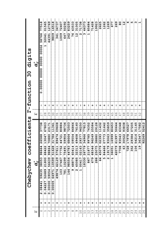
Figure 2: Chebyshev coefficients $\Gamma$-function 30 digits

Figure 2  contains 53 Chebyshev coefficients of the $\Gamma$-function for an accuracy of 30 decimal digits in the whole range $1\leq z\leq\infty$. Using two coefficients the corresponding powerseries is:

[relative error using only 2 coefficients]   [relative error using 11 coefficients]

Figure 3: overall convergence

$$\begin{split}\Gamma\left(z\right)&=\sqrt{2\pi}\cdot z^{z-\frac{1}{2}}\cdot{\rm e}^{-z}*[0.999935+\frac{0.0845506}{z}]\\ \end{split}$$ (6)

the maximal relativ error(Figure 3) is less than $8*10^{-4}$. U̇sing eleven coefficients for the corresponding powerseries

$$\begin{split}\Gamma\left(z\right)&=\sqrt{2\pi}\cdot z^{z-\frac{1}{2}}\cdot{\rm e}^{-z}\\ &\quad*[0.99999999998+\frac{0.083333337647}{z}+\frac{0.0034720552506}{z^{2}}-\frac{0.0026788696285}{z^{3}}\\ &\quad+\frac{0.00024711193390}{z^{4}}+\frac{0.00084986066787}{z^{5}}-\frac{0.000035855790507}{z^{6}}-\frac{0.00068599470338}{z^{7}}\\ &\quad+\frac{0.00067284352663}{z^{8}}-\frac{0.00029536102066}{z^{9}}+\frac{0.000052647439438}{z^{10}}]\end{split}$$ (7)

the maximal relativ error(Figure 3) is less than $2*10^{-11}$.

2.1 The $\Gamma^{-1}$ Function

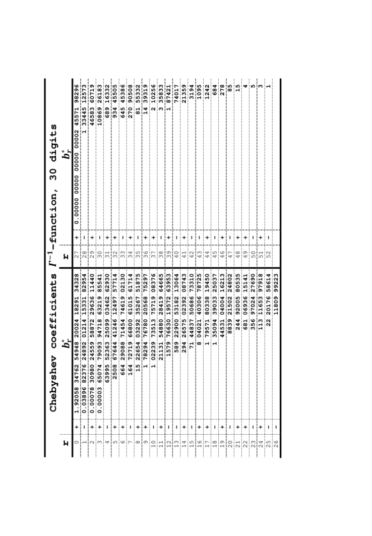
Figure 4: Chebyshev coefficients $\Gamma^{-1}$-function 30 digits

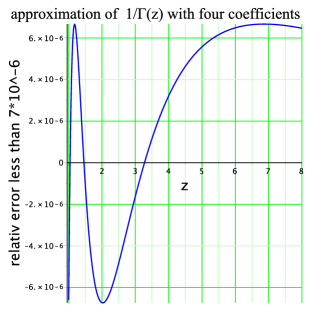
Figure 5: $\Gamma^{-1}$-function error analysis

Figure 4 contains 53 Chebyshev coefficients of the $\Gamma^{-1}$-function for an accuracy of 30 decimal digits in the whole range $1\leq z\leq\infty$.

$$\frac{1}{(z-1)!}\,\simeq\Gamma^{-1}\left(z\right)=\frac{1}{\sqrt{2\pi}}\,{z}^{\frac{1}{2}-z}\,{{\rm e}^{z}}\,*\,\sideset{{}_{\,0}^{\infty}}{{}^{{}^{\prime}}}{\sum}b{{}_{r}^{*}}T{{}_{r}^{*}}(\frac{1}{z})\,,\quad 1\leq\leavevmode\nobreak\ z\leavevmode\nobreak\ \leq\infty$$ (8)

With four coefficients the powerseries expansion is:

$$\Gamma^{-1}\left(z\right)=\frac{1}{\sqrt{2\pi}}\,{z}^{\frac{1}{2}-z}\,{{\rm e}^{z}}\,*\,[1.000006-\frac{0.08354413}{z}\,+\frac{0.004512425}{z^{2}}\,+\frac{0.001168239}{z^{3}}]$$ (9)

The maximal relativ error (Figure 5) is less than $7*10^{-6}$.
In contrast to that in the famous Handbook of Mathematical Functions [2] the series expansion for $\Gamma^{-1}$ is completely wrong.

2.2 The Ln$\Gamma$ Function

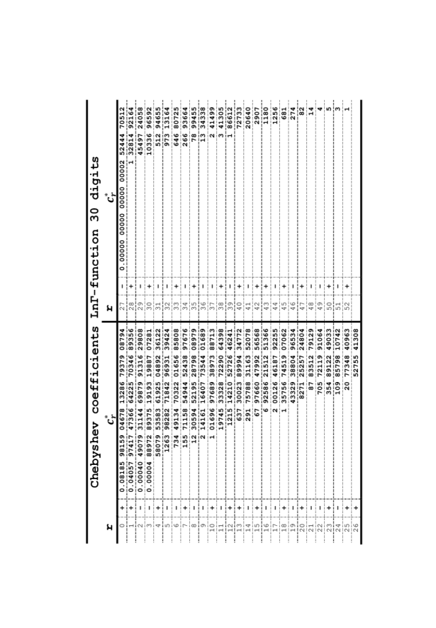
Figure 6: Chebyshev coefficients $ln\Gamma$-function 30 digits

[absolute error using only 2 coefficients]   [absolute error using 5 coefficients]

Figure 7: overall convergence

The approximation is represented by

$$\ln[(z-1)!]\,\simeq\ln\Gamma\left(z\right)=\ln\left(\sqrt{2\pi}\,{z}^{z-\frac{1}{2}}\,{{\rm e}^{-z}}\right)+\sideset{{}_{\,0}^{\infty}}{{}^{{}^{\prime}}}{\sum}c{{}_{r}^{*}}T{{}_{r}^{*}}(\frac{1}{z})\,,\quad 1\leq\leavevmode\nobreak\ z\leavevmode\nobreak\ \leq\infty$$ (10)

Figure 6 contains the Chebyshev coefficients with a precision of 30 decimal digits for the whole range of $1\leq\leavevmode\nobreak\ z\leavevmode\nobreak\ \leq\infty$. Using only the first two coefficients and building the power series form

$$\ln\Gamma\left(z\right)=\ln\sqrt{2\pi}\,+\left(z-\frac{1}{2}\right)\ln\left(z\right)-z+0.91932+\frac{0.081160}{z}$$ (11)

the maximum absolute error (Figure 7) is less than $5*10^{-4}$. Using five coefficients

$$\begin{split}\ln\Gamma&\left(z\right)=\ln\sqrt{2\pi}\,+\left(z-\frac{1}{2}\right)\ln z\,-z\\ &\quad+0.918935\,+\frac{0.0833326}{z}\,+\frac{0.000037082}{z^{2}}-\frac{0.00305155}{z^{3}}\,+\frac{0.000743418}{z^{4}}\\ \end{split}$$ (12)

the maximum absolute error (Figure 7) is less than $2*10^{-7}$.

3 The Chebyshev Interpolation of the Psi (Digamma) Function

This function is the first derivative of the Ln$\Gamma$ Function:

$$\psi^{(0)}(z)\,=\,\psi(z)=\ln^{{}^{\prime}}\Gamma\left(z\right)=\frac{\Gamma^{{}^{\prime}}(z)}{\Gamma(z)}=ln\,z-\frac{1}{2z}+\sideset{{}_{\,0}^{\infty}}{{}^{{}^{\prime}}}{\sum}c{{}_{r}^{*}}T{{}_{r}^{*^{\prime}}}(\frac{1}{z})\,,\quad 1\leq\leavevmode\nobreak\ z\leavevmode\nobreak\ \leq\infty$$ (13)

After differentiating the sum using eq. 23 and eq. 24 , $-\frac{1}{2z}=-\frac{1}{4}*(T^{*}_{0}(\frac{1}{z})+T^{*}_{1}{(\frac{1}{z})})$  has to be added. The final result is

$$\psi^{(0)}(z)\,=\,\psi(z)=\frac{\Gamma^{{}^{\prime}}(z)}{\Gamma(z)}=ln\,z+\sideset{{}_{\,0}^{\infty}}{{}^{{}^{\prime}}}{\sum}\alpha{{}_{(0)r}^{*}}T{{}_{r}^{*}}(\frac{1}{z})\,,\quad 1\leq\leavevmode\nobreak\ z\leavevmode\nobreak\ \leq\infty$$ (14)

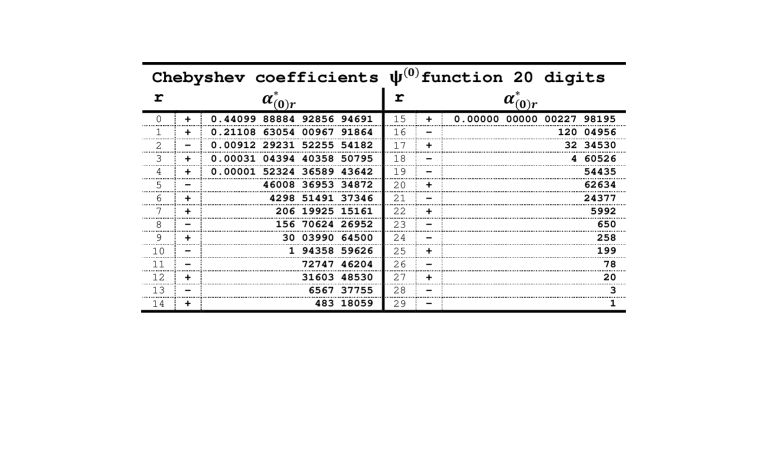
Figure 8: The $\psi^{(0)}$-approximation 20 digits

3.1 Summation of the Harmonic Series

$-\psi^{(0)}(1)\,=\,\gamma\,=0.57721\,\,56649\,\,01532\,\,86061\,\,$is Euler’s constant.

$\psi^{(0)}(n+1)\,-\,\psi^{(0)}(1)\,=\,H_{n}\,=\,1+\frac{1}{2}+\frac{1}{3}+\,...+\frac{1}{n}\,,\quad n\in N$

defines and computes the n-th harmonic number $H_{n}$.

4 Interpolating further Polygamma Functions

Differentiating the result of eq. 14 as before one gets

$$\psi^{(1)}(z)=\psi^{{}^{\prime}}(z)=\frac{1}{z}+\sideset{{}_{\,0}^{\infty}}{{}^{{}^{\prime}}}{\sum}\alpha{{}_{(0)r}^{*}}T{{}_{r}^{*^{\prime}}}(\frac{1}{z})\,,\quad 1\leq\leavevmode\nobreak\ z\leavevmode\nobreak\ \leq\infty$$ (15)

Finally $\frac{1}{z}=\frac{1}{2}*(T^{*}_{0}({\frac{1}{z}})+T^{*}_{1}({\frac{1}{z}}))$ has to be added yielding

$$\psi^{(1)}(z)=\sideset{{}_{\,0}^{\infty}}{{}^{{}^{\prime}}}{\sum}\alpha_{(1)r}^{*}T{{}_{r}^{*}}(\frac{1}{z})\,,\quad 1\leq\leavevmode\nobreak\ z\leavevmode\nobreak\ \leq\infty$$ (16)

The higher Polygamma Functions can be approximated applying the two step differentiation repeatedly without additional correction. Each next generated function looses about two decimal digits in precision.

4.1 Summation of the higher Harmonic Series

The general relation is:

$$\frac{(-1)^{m+1}}{m!}\,\psi^{(m)}(z)=\sum{{}_{k=\,0}^{\infty}}\frac{1}{(z+k)^{m+1}}\,=\,\frac{1}{z^{m+1}}+\frac{1}{(z+1)^{m+1}}+\frac{1}{(z+2)^{m+1}}+...$$ (17)

and especially for z=n integer

$$\frac{(-1)^{m+1}}{m!}\,[\psi^{(m)}(1)-\psi^{(m)}(n)]\,=\,\frac{1}{1^{m+1}}+\frac{1}{2^{m+1}}+\frac{1}{3^{m+1}}+\,...\,+\frac{1}{(n-1)^{m+1}}$$ (18)

and further specialized with m=1

$$\psi^{(1)}(1)-\psi^{(1)}(n)\,=\,\frac{1}{1^{2}}+\frac{1}{2^{2}}+\frac{1}{3^{2}}+\,...\,+\frac{1}{(n-1)^{2}}$$ (19)

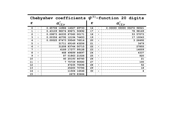
Figure 9: The $\psi^{(1)}$-function 20 digits

5 Relations of the Shifted Chebychev Polynomials

The Shifted Chebyshev polynomials are defined by

$$T^{*}_{r}(\theta) =cos(r\theta)\qquad-1\leq\cos\,\theta\leq+1\quad -1\leq T^{*}_{r}\leq+1$$

$$2z-1 =cos\,\theta\quad 0\leq\leavevmode\nobreak\ z\leavevmode\nobreak\ \leq+1$$

They are power polynomials in z. Their highest coefficient $2^{r-1}$ is used for normalization.
Chebyshev proved [7] that among all normalized power polynomials of same degree (or less) they have the smallest deviation from zero in the range $0\leq z\leq+1$. That makes them unique for optimal interpolation in the declared region. The ranges may be adapted by linear or even nonlinear transformations.
The polynomials for the intervall $0\leq z\leq+1$ are called the shifted polynomials. They are used here exclusively. Explicit expressions for the first few shifted Chebyshev polynomials are: $T^{*}_{0}(z)=1,\quad T^{*}_{1}(z)=2z-1,\quad T^{*}_{2}(z)=8z^{2}-8z+1,\quad T^{*}_{3}(z)=32z^{3}-48z^{2}+18z-1,...$

Inversion gives:
$1=T^{*}_{0}(z),\quad 2z=T^{*}_{0}(z)+T^{*}_{1}(z),\quad 8z^{2}=3T^{*}_{0}(z)+4T^{*}_{1}(z)+T^{*}_{2}(z),\quad\\ 32z^{3}=10\,T^{*}_{0}(z)+15\,T^{*}_{1}(z)+6\,T^{*}_{2}(z)+T^{*}_{3}(z),$…

5.1 Chebychev approximation of smooth functions

$$f(z)=\sideset{{}_{0}^{n}}{{}^{{}^{\prime}}}{\sum}a{{}_{r}^{*}}T{{}_{r}^{*}}(z)=\frac{1}{2}a{{}^{*}_{0}}+a{{}^{*}_{1}}T{{}^{*}_{1}}(z)+a{{}^{*}_{2}}T{{}^{*}_{2}}(z)+a{{}^{*}_{3}}T{{}^{*}_{3}}(z)+...$$ (20)

5.1.1 Numerical determination of the $a{{}_{r}^{*}}$-coefficients

For the given function f(z) the $a{{}_{r}^{*}}$ can be determined by

$$a{{}_{r}^{*}}=\sideset{{}_{j=0}^{m}}{{}^{{}^{\prime\prime}}}{\sum}f(cos^{2}(\frac{j\pi}{2m}))\,cos(\frac{rj\pi}{m})$$ (21)

${}^{{}^{\prime\prime}}$ means: terms with j=0 and j=m must be halfed and m should be chosen sufficiently large
for a good approximation.

5.1.2 Summation

1. substituting the $T^{*}$-polynomials by their powerseries representations and thereafter applying the Horner Scheme or

2. it is better to use the coefficients directly: starting with a sufficiently large index n and applying recursion:
   

   $$b^{*}_{r}=(2*z-1)*b^{*}_{r+1}-b^{*}_{r+2}+a^{*}_{r}\,,\quad b^{*}_{n+1}=b^{*}_{n+2}=0\,,\quad r=n,n-1,...,0$$ (22)

   $f(z)=\frac{1}{2}(b^{*}_{0}-b^{*}_{2})$
   

5.1.3 Differentiation

1. In order to get $f^{{}^{\prime}}(z)=\sideset{{}_{0}^{n-1}}{{}^{{}^{\prime}}}{\sum}a{{}_{r}^{*^{\prime}}}T{{}_{r}^{*}}(z)$ from eq. 20 one starts with a sufficiently large index r=n

   $$a^{*^{\prime}}_{r-1}=a^{*^{\prime}}_{r+1}+4\,r\,a^{*}_{r},\quad a^{*^{\prime}}_{n}=0,\quad a^{*^{\prime}}_{n+1}=0$$ (23)

   and applies the recursion till r=1.

2. Differentiation (chainrule) of $f(x)=\sideset{{}_{\,0}^{n}}{{}^{{}^{\prime}}}{\sum}a{{}_{r}^{*}}T{{}_{r}^{*}}({x})$with $x=\frac{1}{z}$ results in

   $$f^{{}^{\prime}}(z)=-\frac{1}{z^{2}}*\sideset{{}^{n-1}_{0}}{{}^{{}^{\prime}}}{\sum}a{{}_{r}^{*^{\prime}}}T{{}_{r}^{*}}(\frac{1}{z})$$

   
   

   In addition to the former derivation step each coefficient of the derived form has to be multiplied by
   

   $$-\frac{1}{z^{2}}=-(\frac{3}{8}T^{*}_{0}(\frac{1}{z})+\frac{1}{2}T^{*}_{1}(\frac{1}{z})+\frac{1}{8}T^{*}_{2}(\frac{1}{z}))$$ (24)

   applying the multiplication rule of the next subsection.

5.1.4 Multiplication of two Chebyshev approximations

The relation

$$T^{*}_{m}{(z)}*T^{*}_{n}{(z)}=\frac{1}{2}*[T^{*}_{m+n}{(z)}+T^{*}_{|m-n|}{(z)}]$$ (25)

is used for multiplying two polynomials eq. 20. The resulting polynomial has m+n+1 coefficients and may be further reduced in length with a minor loss in accuracy.

References

- [1]
- Abramowitz u. Stegun [1964] \NAT@biblabelnumAbramowitz u. Stegun 1964 Abramowitz, Milton (Hrsg.) ; Stegun, Irene A. (Hrsg.): Handbook of Mathematical Functions with Formulas, Graphs, and Mathematical Tables. U.S. Government Printing Office, Washington, D.C., 1964 (National Bureau of Standards Applied Mathematics Series 55). – xiv+1046 S. – Corrections appeared in later printings up to the 10th Printing, December, 1972. Reproductions by other publishers, in whole or in part, have been available since 1965.
- Clenshaw [1962] \NAT@biblabelnumClenshaw 1962 Clenshaw, C. W.: Chebyshev Series for Mathematical Functions. London : Her Majesty’s Stationery Office, 1962 (National Physical Laboratory Mathematical Tables, Vol. 5. Department of Scientific and Industrial Research). – iv+36 S.
- Graham u. a. [1994] \NAT@biblabelnumGraham u. a. 1994 Graham, Ronald L. ; Knuth, Donald E. ; Patashnik, Oren: Concrete Mathematics: A Foundation for Computer Science. 2nd. Reading, MA : Addison-Wesley Publishing Company, 1994. – xiv+657 S. – ISBN 0–201–55802–5
- Lanczos [1964] \NAT@biblabelnumLanczos 1964 Lanczos, Cornelius: A Precision Approximation of the Gamma Function. (1964)
- Lanczos [1972] \NAT@biblabelnumLanczos 1972 Lanczos, Cornelius ; Bennett, Dr. Albert A. (Hrsg.): Applied Analysis. Prentice Hall, Inc., 1972 (PRENTICE-HALL MATHEMATICS SERIES)
- Natanson [1955] \NAT@biblabelnumNatanson 1955 Natanson, Isidor P.: Konstruktive Funktionentheorie. Akademie-Verlag Berlin, 1955
- Snyder [1966] \NAT@biblabelnumSnyder 1966 Snyder, Martin A.: Chebyshev Methods in Numerical Approximation. PRENTICE-HALL, INC., 1966 (Series in Automatic Computation)
- Temme [1996] \NAT@biblabelnumTemme 1996 Temme, Nico M.: Special Functions: An Introduction to the Classical Functions of Mathematical Physics. New York : John Wiley & Sons Inc., 1996. – xiv+374 S. – ISBN 0–471–11313–1
- Whittaker u. Watson [1927] \NAT@biblabelnumWhittaker u. Watson 1927 Whittaker, E. T. ; Watson, G. N.: A Course of Modern Analysis. 4th. Cambridge University Press, 1927. – Reprinted in 1996. Table errata: Math. Comp. v. 36 (1981), no. 153, p. 319.