The Entire Virial Radius of the Fossil Cluster RXJ1159+5531: II. Dark Matter and Baryon Fraction

Abstract

In this second paper on the entire virial region of the relaxed fossil cluster RXJ 1159+5531 we present a hydrostatic analysis of the azimuthally averaged hot intracluster medium (ICM) using the results of Paper 1 (Su et al. 2015). For a model consisting of ICM, stellar mass from the central galaxy (BCG), and an NFW dark matter (DM) halo, we obtain a good description of the projected radial profiles of ICM emissivity and temperature that yield precise constraints on the total mass profile. The BCG stellar mass component is clearly detected with a $K$-band stellar mass-to-light ratio, $M_{\star}/L_{K}=0.61\pm 0.11\,M_{\odot}/L_{\odot}$, consistent with stellar population synthesis models for a Milky-Way IMF. We obtain a halo concentration, $c_{200}=8.4\pm 1.0$, and virial mass, $M_{200}=(7.9\pm 0.6)\times 10^{13}\,M_{\odot}$. For its mass, the inferred concentration is larger than most relaxed halos produced in cosmological simulations with Planck parameters, consistent with RXJ 1159+5531 forming earlier than the general halo population. The baryon fraction at $r_{200}$, $f_{\rm b,200}=0.134\pm 0.007$, is slightly below the Planck value (0.155) for the universe. However, when we take into account the additional stellar baryons associated with non-central galaxies and the uncertain intracluster light (ICL), $f_{\rm b,200}$ increases by $\approx 0.015$, consistent with the cosmic value and therefore no significant baryon loss from the system. The total mass profile is nearly a power law over a large radial range ($\sim 0.2$-10 $R_{e}$), where the corresponding density slope $\alpha$ obeys the $\alpha-R_{e}$ scaling relation for massive early-type galaxies. Performing our analysis in the context of MOND still requires a large DM fraction ($85.0\%\pm 2.5\%$ at $r=100$ kpc) similar to that obtained using the standard Newtonian approach. The detection of a plausible stellar BCG mass component distinct from the NFW DM halo in the total gravitational potential suggests that $\sim 10^{14}\,M_{\odot}$ represents the mass scale above which dissipation is unimportant in the formation of the central regions of galaxy clusters.

1. Introduction

It is well appreciated that galaxy clusters are powerful tools for cosmological studies, especially through their halo mass function and global baryon fractions (e.g., Allen et al. 2011; Kravtsov & Borgani 2012). In order to obtain mass measurements of ever larger numbers of cluster masses at higher redshifts, studies must resort to global scaling relations, often involving proxies for the mass. Global scaling relations of ICM properties are particularly useful to probe cooling and feedback in cluster evolution. Measurements of global scaling relations must be interpreted within the context of a general paradigm (e.g., $\Lambda$CDM) that makes definite assumptions about the full radial structure of a halo. It is essential that those assumptions be verified for as many systems as possible through detailed radial mapping of halo properties.

Fortunately, there are several powerful probes of cluster mass distributions (e.g., galaxy kinematics, ICM temperature and density profiles, gravitational lensing, SZ effect) which, ideally, can be combined to achieve the most accurate picture of cluster structure (e.g., Reiprich et al. 2013). In practice, different techniques are better suited for particular clusters because of multiple factors, such as distance and mass.

Well-known advantages of studying the ICM include (1) that it traces the three-dimensional cluster potential well; (2) the electron mean free path is sufficiently short (especially when considering the presence of weak magnetic fields) to guarantee the fluid approximation holds (i.e., with an isotropic pressure tensor); and (3) the hydrostatic equilibrium approximation should apply within the virialized region, allowing the gravitating mass to be derived directly from the temperature and density profiles of the ICM (e.g., Sarazin 1986; Ettori et al. 2013).

Since clusters are still forming in the present epoch, deviations from the hydrostatic approximation are expected. Cosmological simulations expect typically 10%-30% of the total ICM pressure is non-thermal, primarily arising from random turbulent motions (e.g., Rasia et al. 2004; Nagai et al. 2007; Eckert et al. 2015). Even with the very unfortunate demise of Astro-H, eventually microcalorimeter detectors will provide for the first time precise direct measurements of ICM kinematics for many bright clusters, greatly reducing (or eliminating) this greatest source of systematic error in ICM studies (e.g., Kitayama et al. 2014). Even so, for the most reliable hydrostatic analysis it is desirable that the correction for non-thermal pressure be as small as possible; i.e., for the most relaxed systems.

It turns out to be difficult to find clusters with undisturbed ICM within their entire virial region. The clusters that tend to be the most dynamically relaxed over most of their virial region are the cool core clusters which, unfortunately, are also those that most often display ICM disturbances in their central regions believed to arise from intermittent feedback from an AGN in the central galaxy (e.g., Bykov et al. 2015). Hence, CC clusters with the least evidence for central ICM disturbance are probably the best clusters for hydrostatic studies.

The cool core fossil cluster RXJ 1159+5531 is especially well-suited for hydrostatic studies of its ICM. It is both sufficiently bright and distant $(z=0.081)$ allowing for its entire virial region to be mapped through a combination of Chandra and Suzaku observations with feasible total exposure time. The high-quality Chandra image reveals a highly regular ICM with no evidence of large, asymmetrical disturbances anywhere, including the central regions (Humphrey et al. 2012a). We have Suzaku observations covering the entire region within $r_{200}$ on the sky and presented results for the ICM properties in each of four directions (including using the central Chandra observation) in Su et al. (2015, hereafter Paper 1). We found the ICM properties (e.g, temperature, density) to display only very modest azimuthal variations ($<10\%$), providing evidence for a highly relaxed ICM.

In this second paper on the entire virial radius of RXJ 1159+5531 we focus on measurements of the BCG stellar mass-to-light ratio, dark matter, gas, and baryon fraction. Whereas Paper 1 focused on the comparison of ICM properties obtained for each of the four directions observed by Suzaku, here we analyze results for all the directions together to obtain the best-fitting azimuthally averaged ICM and mass properties. For calculating distances we assumed a flat $\Lambda$CDM cosmology with $\Omega_{m,0}=0.3$ and $H_{0}=70$ km s^-1 Mpc^-1. At the redshift of RXJ 1159+5531 ($z=0.081$) this translates to an angular-diameter distance of $315$ Mpc and $1\arcsec=1.5$ kpc. Unless stated otherwise, all statistical uncertainties quoted in this paper are $1\sigma$.

The paper is organized as follows. We review very briefly the observations, data preparation, and ICM measurements in §2. We discuss our implementation of the hydrostatic method in §3 and define the particular models and parameters in §4. We present the results in §5 and describe the construction of the systematic error budget in §6. Finally, in §7 we discuss several implications of our results and present our summary and conclusions in §8.

2. Observations

The observations and data preparation are reported in Paper 1, and we refer the interested reader to that paper for details. Briefly, after obtaining cleaned events files for each observation, we extracted spectra in several concentric circular annuli for each data set and constructed appropriate response files for each annulus; i.e., redistribution matrix files (RMFs) and auxiliary response files (ARFs, including “mixing” ARFs to account for the large, energy-dependent Point Spread Function of the Suzaku data). We constructed model Suzaku spectra representing the “non-cosmic” X-ray background (NXB) and subtracted these from the observations. All other background components for both the Chandra and Suzaku data were accounted for with simple parameterized models fitted directly to the observations using xspec v12.7.2 (Arnaud 1996); i.e., the annular spectrum of each data set was fitted individually with a complex spectral model consisting of components for the ICM and background. For each annulus on the sky a single thermal plasma component (vapec) was fitted to represent all the ICM emission in that annulus. No deprojection was performed during the spectral fitting because it amplifies noise and renders the analysis of the background-dominated cluster outskirts even more challenging. Furthermore, standard deprojection algorithms (e.g., onion-peeling and projct in xspec) do not generally account for ICM emission outside the bounding annulus, which also can lead to sizable systematic effects (e.g., Nulsen & Bohringer 1995; McLaughlin 1999; Buote 2000a).

Consequently, the principal data products resulting from our analysis are the radial profiles of projected (1) emission-weighted temperature and (2) emissivity-weighted $\rho_{\rm gas}^{2}$; e.g., equations B10 and B13 of Gastaldello et al. (2007). In addition, we also use the profile of projected, emission-weighted iron abundance ($Z_{\rm Fe}$) expressed in solar units (Asplund et al. 2006) to further constrain the emissivity in our hydrostatic models.

3. Entropy-Based Method

We prefer to construct hydrostatic equilibrium models using an approach that begins by specifying a parameterized model for the ICM entropy (Humphrey et al. 2008). The benefits of this “entropy-based” approach, as well as a review of other methods, are presented in Buote & Humphrey (2012a). Compared to the temperature and density, the entropy profile is more slowly varying and has a well-motivated asymptotic form, $\sim r^{1.1}$ for all clusters (e.g., Tozzi & Norman 2001; Voit et al. 2005). In addition, by requiring the entropy to be a monotonically increasing function of radius, the additional contraint of convective stability (not typically applied in cluster mass studies) is easily enforced. We assume spherical symmetry which, if in fact the cluster is a triaxial ellipsoid, introduces only modest biases into the inferred parameters (see §6.1).

For studies of cluster ICM the thermodynamic entropy is usually replaced by the entropy proxy, $S\equiv k_{\rm B}Tn_{e}^{-2/3},$ expressed in units of keV cm². It is useful to define the quantity, $S_{\rho}\equiv(k_{\rm B}/\mu m_{\rm a})T\rho_{\rm gas}^{-2/3},$ where $\mu$ is the mean atomic mass of the ICM and $m_{a}$ is the atomic mass unit, that replaces $n_{e}$ in the entropy proxy with $\rho_{\rm gas}$ (e.g., using eqn. B4 of Gastaldello et al. 2007) so that,

$$\frac{S_{\rho}}{S}=\frac{1}{\mu m_{\rm a}}\left(\frac{2+\mu}{5\mu}\frac{1}{m_{\rm a}}\right)^{2/3}.$$ (1)

The equation of hydrostatic equilibrium may now be written,

$$\frac{d\xi}{dr}=-\frac{2}{5}\frac{GM(<r)}{r^{2}}S_{\rho}^{-3/5}$$ (2)

where $\xi\equiv P^{2/5}$, $P$ is the total thermal pressure, and $M(<r)$ is the total gravitating mass enclosed within radius $r$. Given $S_{\rho}$ (after specifying $S$) and $M(<r)$, the hydrostatic equation can be integrated directly to obtain $\xi$ and therefore the profiles of gas density, $\rho_{\rm gas}=(P/S_{\rho})^{3/5}=S_{\rho}^{-3/5}\xi^{3/2}$, and temperature, $k_{\rm B}T/\mu m_{\rm a}=S_{\rho}^{3/5}P^{2/5}=S_{\rho}^{3/5}\xi$. By comparing the density and temperature profiles to the observations, we constrain the parameters of the input $S$ and $M(<r)$ models.

Since $M(<r)$ in eqn. (2) contains $M_{\rm gas}$, direct integration only yields a self-consistent solution for $\rho_{\rm gas}$ provided $M_{\rm gas}\ll M(<r).$ In Paper 1, and all our previous studies of the entropy-based method, we insured self-consistency in the case where $M_{\rm gas}$ cannot be neglected by differentiating the equation with respect to r and making use of the equation of mass continuity; e.g., see eqn. (4) of Paper 1. Here we instead employ an iterative solution of eqn. (2) by treating $M_{\rm gas}$ as a small perturbation. We solve eqn. (2) initially by setting $M_{\rm gas}=0$. From this solution we use the new $\rho_{\rm gas}$ to compute the profile of $M_{\rm gas}$. We then insert it into the hydrostatic equation and obtain an improved solution. The process is repeated until the value of $M_{\rm gas}$ near the virial radius changes by less than a desired amount.

A boundary condition on $\xi$ must be specified to obtain a unique solution of eqn. (2). We choose to specify the “reference pressure,” $P_{\rm ref}$, at a radius of 10 kpc. Hence, the free parameters in our hydrostatic model are $P_{\rm ref}$ and those associated with $S$ and $M(<r)$, which we detail below in §4.

To compare to the observations, the three-dimensional density and temperature profiles of the ICM obtained from eqn. (2) are used to construct the volume emissivity, $\epsilon_{\nu}\propto\rho_{\rm gas}^{2}\Lambda_{\nu}(T,Z)$, where $\Lambda_{\nu}(T,Z)$ is the ICM plasma emissivity. Then $\epsilon_{\nu}$ and the emission-weighted temperature are projected on to the sky and averaged over the various circular annuli corresponding to the X-ray data using equations B10 and B13 of Gastaldello et al. (2007). Since $\Lambda_{\nu}(T,Z)$ also depends on the metal abundances, we need to specify the abundance profiles in our models. As in our previous studies, we obtain best results by simply using the measured abundance profiles in projection and assigning them to be the true three-dimensional profiles for the models. (The iron abundance profiles are presented in Fig. 3 of Humphrey et al. 2012a and Fig. 13 of Paper 1.) In §6.8 we discuss instead using a parameterized model for the iron abundance that is emission-weighted and projected onto the sky and fitted to the observations.

Since the X-ray emission in each annulus on the sky generally contains the sum of a range of temperatures and metallicities owing to radial gradients in the ICM properties, the values in particular of the temperature and metallicity obtained by fitting single-component ICM models to the projected spectra can be substantially biased with respect to the emission-weighted values (e.g., Buote 2000b; Mazzotta et al. 2004). To partially mitigate such biases in the data-model comparison, we employ “response weighting” of our projected models (see eqn. B15 of Gastaldello et al. 2007).

4. Models and Parameters

4.1. Entropy

For the ICM entropy profile we employ a power-law with two breaks plus a constant,

$$S(r)=s_{0}+s_{1}f(r),$$ (3)

where $s_{0}$ represents a constant entropy floor, and $s_{1}=S(r_{\rm ref})-s_{0}$ for some reference radius $r_{\rm ref}$ (taken to be 10 kpc). The dimensionless function $f(r)$ is,

$$f(r)=\left\{\begin{array}[]{l}\left(\frac{r}{r_{\rm ref}}\right)^{\alpha_{1}}\hfill r\leq r_{\rm b,1}\\ f_{1}\left(\frac{r}{r_{\rm ref}}\right)^{\alpha_{2}}\qquad\qquad\hfill r_{\rm b,1}<r\leq r_{\rm b,2}\\ f_{2}\left(\frac{r}{r_{\rm ref}}\right)^{\alpha_{3}}\hfill r>r_{\rm b,2}\end{array}\right.\$$

where $r_{\rm b,1}$ and $r_{\rm b,2}$ are the two break radii, and the coefficients $f_{1}$ and $f_{2}$ are given by,

$$f_{n}=f_{n-1}\left(\frac{r_{{\rm b},n}}{r_{\rm ref}}\right)^{\alpha_{n}-\alpha_{n+1}},$$

with $f_{0}\equiv 1.$ To enforce convective stability (§3) we require $\alpha_{1},\alpha_{2},\alpha_{3}\geq 0.$ Hence, this model has seven free parameters: $s_{0}$, $s_{1}$, $r_{\rm b,1}$, $r_{\rm b,2}$, $\alpha_{1}$, $\alpha_{2}$, and $\alpha_{3}$.

4.2. Stellar Mass

We represent the stellar mass of the cluster using the $K$-band light profile of the BCG (2MASX J11595215+5532053) from the Two Micron All-Sky Survey (2MASS) as listed in the Extended Source Catalog (Jarrett et al. 2000); i.e., an $n=4$ Sersic model (i.e., de Vaucouleurs) with $r_{e}=9.83$ kpc and $L_{K}=1.03\times 10^{12}\,L_{\odot}$. Additional (poorly constrained) stellar mass contributions from non-central galaxies and intracluster light are treated as a systematic error in §6.2.

4.3. Dark Matter

We consider the following models for the distribution of dark matter.

• NFW As it is the current standard both for modeling observations and simulated clusters, we use the NFW profile (Navarro et al. 1997) for our fiducial dark matter model. It has two free parameters, a concentration $c_{\Delta}$, and mass $M_{\Delta}$, evaluated with respect to an overdensity $\Delta$ times the critical density of the universe.

• Einasto The Einasto profile (Einasto 1965) is now recognized as a more accurate representation of the profiles of dark matter halos. We implement the mass profile following Merritt et al. (2006) but using the approximation for $d_{n}$ given by Retana-Montenegro et al. (2012). As with the NFW profile, we express the parameters of the Einasto model in terms of a virial concentration, $c_{\Delta}$, and mass, $M_{\Delta}$. We fix $n=5\,(\alpha=0.2)$ appropriate for cluster halos (e.g., Dutton & Macciò 2014).

• CORELOG To provide a strong contrast to the NFW and Einasto models, we investigate a model having a constant density core and with a density that approaches $r^{-2}$ at large radius. For consistency, we also express the free parameters of this model in terms of a virial concentration, $c_{\Delta}$, and mass, $M_{\Delta}$; e.g., see §2.1.2 of Buote & Humphrey (2012b) for more details.

All $c_{\Delta}$, $M_{\Delta}$, and $r_{\Delta}$ values are evaluated at the redshift of RXJ 1159+5531 (i.e., $z=0.081$). Below we quote concentration values for the total mass profile (i.e., stars+gas+DM) as, $c_{\Delta}^{\rm tot}\equiv r_{\Delta}^{\rm tot}/r_{s}^{\rm DM}$, where $r_{s}^{\rm DM}$ is the DM scale radius and $r_{\Delta}^{\rm tot}$ is the virial radius of the total mass profile. We determine $r_{\Delta}^{\rm tot}$ iteratively starting with the DM virial radius, adding in the baryon components, recomputing the virial radius, and stopping when the change in virial radius is less than a desired tolerance.

5. Results

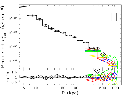
Figure 1.— The quantity plotted (with $1\sigma$ errors) is proportional to the ICM surface brightness divided by $\Lambda_{\nu}(T,Z)$ (see equation B10 of Gastaldello et al. 2007). The best-fitting fiducial hydrostatic model is also over-plotted so that its color reflects its value for each data set. The data sets are labelled as follows: Chandra (black); Suzaku pointings: N (blue), S (red), W (green), E (yellow). The vertical lines in the top right corner indicate the best-fitting virial radii for the fiducial model; i.e., from left to right: $r_{500}$, $r_{200}$, and $r_{108}$. The bottom panel plots the data/model ratio.

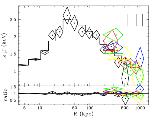
Figure 2.— Projected emission-weighted hot gas temperature ($k_{B}T$) along with the best-fitting fiducial hydrostatic model in each circular annulus versus radius $R$ on the sky. The labeling scheme is the same as Fig. 1

5.1. Overview

We fitted the model to the data using the “nested sampling” Bayesian Monte Carlo procedure implemented in the MultiNest code v2.18 (Feroz et al. 2009), and we adopted flat priors on the logarithms of all the free parameters. We used a $\chi^{2}$ likelihood function, where the $\chi^{2}$ consists of the temperature and projected $\rho_{\rm gas}^{2}$ data points, the model values, and the statistical weights. The weights are the variances of the data points obtained from the spectral fitting in Paper 1. We quote two “best” values for each parameter: (1) “Best Fit”, which is the expectation value of the parameter in the derived posterior probability distribution, and (2) “Max Like”, which is the parameter value that gives the maximum likelihood (found during the nested sampling). Finally, unless stated otherwise, all errors quoted are $1\sigma$ representing the standard deviation of the parameter computed in the posterior probability distribution. All models shown in the figures have been evaluated using the “Max Like” values.

In Figures 1 and 2 we display the projected $\rho_{\rm gas}^{2}$ ($\propto\Sigma_{\nu}/\Lambda_{\nu}(T,Z)$, where $\Sigma_{\nu}$ is the surface brightness) and temperature data along with the best-fitting “fiducial” model (and residuals). The fiducial model consists of an entropy profile with two breaks, the $n=4$ sersic model for the stellar mass of the BCG, and the NFW model for the dark matter. Inspection of the figures reveals that, overall, the fit is good. Most of the fit residuals are within $\approx 1\sigma$ of the model values, and the most deviant points lie within $\approx 2\sigma$ of the model values. Since for our Bayesian analysis we cannot easily formally assess the goodness-of-fit as in a frequentist approach, we have also fitted models to the data using a standard frequentist $\chi^{2}$ analysis. For our fiducial model we obtain a minimum $\chi^{2}=39.9$ for 39 degrees of freedom, which is formally acceptable from the frequentist perspective. (For reference, if the BCG component is omitted, $\chi^{2}=59.6$; i.e., the data strongly require it.)

Below we shall often refer to the “Best Fit” virial radii of the fiducial model: $r_{2500}=271$ kpc, $r_{500}=575$ kpc, $r_{200}=862$ kpc, and $r_{\rm vir}=r_{108}=1.12$ Mpc.

5.2. Entropy

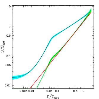
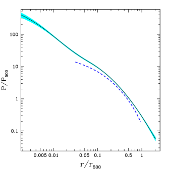
Figure 3.— (Left Panel) Radial entropy profile (black) and $1\sigma$ error region (cyan) for the fiducial hydrostatic model expressed in terms of the characteristic value $S_{500}$. The red line indicates the baseline $r^{1.1}$ profile produced by gravity-only cosmological simulations (Voit et al. 2005). The black dashed line (and green $1\sigma$ region) represents rescaling the entropy profile by a function of the gas fraction according to Pratt et al. (2010). (Right Panel) Pressure profile (black) compared to the universal profile inferred for groups and clusters by Arnaud et al. (2010) which is expected to apply for the radii shown.

Table 1Pressure and Entropy

	$P_{\rm ref}$	$s_{0}$	$s_{1}$	$r_{\rm b,1}$	$r_{\rm b,2}$	$\alpha_{1}$	$\alpha_{2}$	$\alpha_{3}$
	($10^{-2}$ keV cm-3)	(keV cm2)	(keV cm2)	(kpc)	(kpc)
Best Fit	$5.30\pm 0.25$	$4.48\pm 0.78$	$10.9\pm 1.3$	$35.6\pm 5.1$	$708\pm 277$	$1.81\pm 0.18$	$0.57\pm 0.06$	$1.01\pm 0.44$
(Max Like)	$(5.49)$	$(4.51)$	$(10.7)$	$(42.4)$	$(180)$	$(1.80)$	$(0.36)$	$(0.74)$

The results for the entropy profile using the fiducial hydrostatic model are displayed in Fig. 3, and the parameter constraints are listed in Table 1. In the figure we have plotted the “scaled” entropy in units of the characteristic entropy, $S_{500}=260.6$ keV cm² (see eqn. 3 of Pratt et al. 2010). The entropy profile has a small, but significant floor at the center and then rises more steeply than the $\sim r^{1.1}$ profile out to the first break radius ($\approx 36$ kpc). The profile is then shallower than the baseline model out to the second break ($\approx 700$ kpc), after which the slope is uncertain, but consistent with the baseline model out to the largest radii investigated $(\sim r_{\rm 108})$. As noted in Paper 1, at no radius does the scaled entropy fall below the baseline model, consistent with a simple feedback explanation. (See Paper 1 for more detailed discussion of how the entropy profile compares to theoretical models.)

In Fig. 3 following Pratt et al. (2010) we also show the result of rescaling the entropy profile by $(f_{\rm gas}/f_{b,U})^{2/3}$, where $f_{\rm gas}$ is the gas fraction as a function of radius and $f_{b,U}=0.155$ is the baryon fraction of the Universe. The overall very good agreement of this rescaled entropy profile with the baseline model suggests that the feedback has primarily served to spatially redistribute the gas rather than raise its temperature.

We note that the second break in the entropy profile is not required at high significance; i.e., the ratio of the Bayesian evidences for the 2-break and 1-break model is 1.9.

5.3. Pressure

The results for the pressure profile using the fiducial hydrostatic model are displayed in Fig. 3, and the constraints for the reference pressure are listed in Table 1. In the figure we have plotted the “scaled” pressure in units of the characteristic pressure, $P_{500}=5.9\times 10^{-4}$ keV cm^-3 (see eqn. 5 of Arnaud et al. 2010), and compared to the “universal” pressure profile of Arnaud et al. (2010). (Note that we quote results for the total gas pressure rather than the electron gas pressure and have accounted for this also in the definition of $P_{500}$.) In most of the region where the universal profile is expected to be valid, the pressure profile of RXJ 1159+5531 agrees within the 20% scatter in the pressure profiles of the clusters studied by Arnaud et al. (2010), reaching maximum deviations of 50-60% at the endpoints; i.e., RXJ 1159+5531 has a pressure profile similar to the other clusters.

5.4. Mass

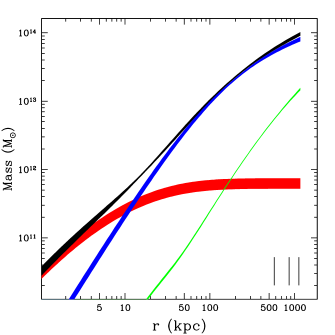
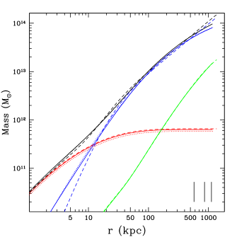
Figure 4.— (Left Panel) Radial profiles of the various mass components of the fiducial hydrostatic model: total mass (black), NFW DM (blue), stars (red), hot gas (green). The vertical lines in the bottom right corner indicate the best-fitting virial radii for the fiducial model; i.e., from left to right: $r_{500}$, $r_{200}$, and $r_{108}$. (Right Panel) Results shown for hydrostatic models having different dark matter profiles: NFW (solid lines), Einasto (dotted lines), Corelog (dashed lines). Only the best-fitting models are shown. The color scheme is the same as for the left panel. The gas mass profiles are indistinguishable between the models.

Table 2Stellar and Total Mass

	$M_{\star}/L_{K}$	$c_{2500}$	$M_{2500}$	$c_{500}$	$M_{500}$	$c_{200}$	$M_{200}$	$c_{\rm vir}$	$M_{\rm vir}$
	($M_{\odot}L_{\odot}^{-1}$)		($10^{13}M_{\odot}$)		($10^{13}M_{\odot}$)		($10^{13}M_{\odot}$)		($10^{13}M_{\odot}$)
Best Fit	$0.61\pm 0.11$	$2.6\pm 0.4$	$3.1\pm 0.1$	$5.6\pm 0.7$	$5.9\pm 0.4$	$8.4\pm 1.0$	$7.9\pm 0.6$	$10.9\pm 1.3$	$9.4\pm 0.7$
(Max Like)	$(0.53)$	$(3.0)$	$(3.1)$	$(6.3)$	$(5.6)$	$(9.4)$	$(7.4)$	$(12.2)$	$(8.8)$
Spherical	$\cdots$	$\cdots$	$\cdots$	${}_{-0.32}^{+0.13}$	${}_{-0.04}^{+0.15}$	$\cdots$	$\cdots$	$\cdots$	$\cdots$
Einasto	$-0.05$	$-0.2$	$-0.0$	$-0.4$	$0.1$	$-0.6$	$0.1$	$-0.9$	$0.1$
CORELOG	$-0.05$	$10.0$	$-0.4$	$23.1$	$0.5$	$37.5$	$2.4$	$51.7$	$4.7$
1 Break	$0.02$	$-0.1$	$0.0$	$-0.2$	$0.1$	$-0.2$	$0.2$	$-0.3$	$0.2$
$\Lambda_{\nu}(T,Z)$	$-0.04$	$0.2$	$-0.1$	$0.5$	$-0.4$	$0.7$	$-0.5$	$0.9$	$-0.6$
Response	$0.02$	$-0.2$	$0.0$	$-0.4$	$0.1$	$-0.6$	$0.3$	$-0.8$	$0.3$
Proj. Limit	${}^{+0.00}_{-0.00}$	${}^{+0.0}_{-0.0}$	${}^{+0.0}_{-0.0}$	${}^{+0.0}_{-0.0}$	${}^{+0.0}_{-0.0}$	${}^{+0.1}_{-0.0}$	${}^{+0.0}_{-0.0}$	${}^{+0.1}_{-0.0}$	${}^{+0.0}_{-0.0}$
SWCX	$0.00$	$-0.0$	$0.0$	$-0.0$	$0.0$	$-0.1$	$0.1$	$-0.1$	$0.1$
Distance	${}^{+0.03}_{-0.02}$	${}^{+0.1}_{-0.1}$	${}^{+0.0}_{-0.0}$	${}^{+0.1}_{-0.2}$	${}^{+0.1}_{-0.1}$	${}^{+0.2}_{-0.3}$	${}^{+0.1}_{-0.1}$	${}^{+0.2}_{-0.3}$	${}^{+0.2}_{-0.2}$
$N_{\rm H}$	$-0.02$	$0.1$	$-0.0$	$0.2$	$-0.1$	$0.3$	$-0.2$	$0.4$	$-0.3$
Fix $Z_{\rm Fe}(r_{\rm out})$	${}^{+0.05}_{-0.03}$	${}^{+0.2}_{-0.3}$	${}^{+0.2}_{-0.1}$	${}^{+0.3}_{-0.5}$	${}^{+0.5}_{-0.2}$	${}^{+0.5}_{-0.8}$	${}^{+0.7}_{-0.3}$	${}^{+0.6}_{-1.1}$	${}^{+0.8}_{-0.4}$
Solar Abun.	$-0.05$	$0.3$	$-0.1$	$0.5$	$-0.3$	$0.7$	$-0.5$	$1.0$	$-0.6$
PSF	$0.03$	$-0.1$	$0.1$	$-0.3$	$0.2$	$-0.4$	$0.3$	$-0.5$	$0.4$
FI-BI	$0.02$	$-0.1$	$-0.0$	$-0.1$	$0.0$	$-0.2$	$0.1$	$-0.2$	$0.1$
NXB	${}^{+0.01}_{-0.00}$	$-0.0$	${}^{+0.1}_{-0.0}$	$-0.0$	${}^{+0.1}_{-0.0}$	$-0.1$	$0.1$	$-0.1$	${}^{+0.1}_{-0.0}$
CXB	$-0.01$	$0.0$	$0.0$	$0.1$	$-0.0$	$0.1$	$-0.0$	$0.1$	$-0.1$
CXBSLOPE	${}^{+0.06}_{-0.04}$	${}^{+0.2}_{-0.4}$	${}^{+0.3}_{-0.1}$	${}^{+0.4}_{-0.7}$	${}^{+0.8}_{-0.4}$	${}^{+0.7}_{-1.0}$	${}^{+1.1}_{-0.5}$	${}^{+0.9}_{-1.4}$	${}^{+1.2}_{-0.6}$

In Fig. 4 we show the profiles for the total mass and different mass components for the fiducial hydrostatic model, while in Table 2 we list the results for $M_{\star}/L_{K}$ and the NFW parameters, concentration and mass, evaluated for several over-densities. Of all the mass components, the stellar mass has the weakest constraints $(\sim\pm 18\%)$, while the gas mass is the best constrained (e.g., $\sim\pm 4\%$ at $r_{\rm 108}$.), considering only the statistical errors.

Most of the possible systematic errors we consider in §6, and listed in Table 2, are not significant since they induce parameter changes of the same size or smaller than the $1\sigma$ statistical error. The most significant changes result from aspects of the background modeling (§6.6), the treatment of the plasma emissivity (§6.8), and how the metal abundances are treated (§6.5), particularly in the outermost apertures; i.e., the CXBSLOPE, $\Lambda_{\nu}(T,Z)$, Solar Abun, and Fix $Z_{\rm Fe}(r_{\rm out})$ rows in Table 2. It is, however, reassuring that even these changes generally lead to parameter changes not much larger than $1\sigma$. (See §6 for a more detailed discussion of the systematic error budget.)

The value we obtain for the $K$-band stellar mass-to-light ratio ($M_{\star}/L_{K}\approx 0.6M_{\odot}/L_{\odot}$) of the BCG agrees very well with our previous determinations (Gastaldello et al. 2007; Humphrey et al. 2012a) and also is consistent with the value expected from stellar population synthesis models. Using the published relationship between stellar mass-to-light ratio and color from Zibetti et al. (2009), we obtain $M_{\star}/L_{K}\approx 0.55M_{\odot}/L_{\odot}$ for $g-i=1.41$, where the $g$ and $i$ magnitudes are taken from the “Model” entries in the NASA/IPAC Extragalactic Database (NED) referring to the Sloan Digital Sky Survey Data Release 6 . This good agreement should be considered only a mild consistency check, since (1) there is significant scatter depending on which bands are used for the color (we used $g-i$ as favored by Zibetti et al. 2009), and (2) the relationship between color and $M_{\star}/L_{K}$ depends on the assumed stellar initial mass function (IMF). If instead we use the relationship between stellar mass-to-light-ratio and color of Bell et al. (2003), who employ a Salpeter-like IMF, we obtain $M_{\star}/L_{K}\approx 0.94M_{\odot}/L_{\odot}$, about $3\sigma$ above our measured value. While there is considerable scatter depending on the color used, the X-ray analysis favors the lower $M_{\star}/L_{K}$ obtained from Zibetti et al. (2009) who adopt a Milky-Way IMF (Chabrier 2003). Several previous studies have found that massive early-type galaxies instead favor a Salpeter IMF (e.g., Conroy & van Dokkum 2012; Newman et al. 2013a; Dutton & Treu 2014), although the more recent study by (e.g. Smith et al. 2015) and most of our previous X-ray studies (e.g., Humphrey et al. 2009, 2012b) favor a Milky-Way IMF.

Since fossil clusters like RXJ 1159+5531 are thought to be highly evolved, early forming systems, it is interesting to examine whether they possess large concentrations for their mass compared to the general population. According to the results of Dutton & Macciò (2014), the mean value of $c_{200}$ for a “relaxed” dark matter halo with $M_{200}=7.9\times 10^{13}\,M_{\odot}$ in the Planck cosmology is 5.3, which is a little more than $3\sigma$ lower than the value we measure for RXJ 1159+5531 $(8.4\pm 1.0)$. In addition, with respect to the intrinsic scatter of the theoretical relation, the $c_{200}$ value is a $\sim 2\sigma$ outlier. Hence, with respect to the fiducial hydrostatic model with an NFW DM halo, RXJ 1159+5531 appears to possess a significantly above-average concentration, consistent with forming earlier than the average halo population. For the Einasto DM halo, our measured $c_{200}=7.8\pm 1.0$ is slightly more than $2\sigma$ above the mean predicted value of 5.6 and a little above the $1\sigma$ intrinsic scatter ($c_{200}=7.5$) using the results of Dutton & Macciò (2014). The reduced significance for the Einasto case arises from a combination of our smaller measured $c_{200}$ and also larger theoretical intrinsic scatter for the Einasto profile compared to NFW.

In the right panel of Fig. 4 we compare the results for the different dark matter models. As is readily apparent from visual inspection, the gas mass profiles are virtually identical for all three cases; i.e., the inferred gas mass profile is robust to the assumed dark matter model. Over most of the radii investigated, the total mass profile is also quite insensitive to the assumed dark matter model, though CORELOG leads to a more massive halo than either NFW or Einasto. (Note in particular the “pinching” of the total mass profile near 10-20 kpc, about 1-2 $R_{e}$, where the dark matter crosses over the stellar mass.) The largest deviations appear at the very largest radii ($\gtrsim r_{108}$). The fitted stellar mass profile is very similar for all three DM models and yields consistent $M_{\star}/L_{K}$ values in each case.

All the DM models produce fits of similar quality in terms of the magnitude of their fractional residuals. When we perform a frequentist $\chi^{2}$ fit we obtain minimum $\chi^{2}$ values of 39.4 for Einasto, 40.1 and for CORELOG compared to 39.9 for NFW; i.e., the fits are statistically indistinguishable from the frequentist perspective. Moreover, from the Bayesian analysis we can use the ratio of evidences to compare the Einasto $(\ln Z=-53.00)$ and NFW $(\ln Z=-53.81)$ models since they have essentially the same free parameters and priors: We obtain an evidence ratio of 2.2 in favor of the Einasto model, which is not very significant. It is not straightforward to compare the evidences of the CORELOG and NFW models because they have different prior volumes (and the models are not “nested”). Nevertheless, the frequentist minimum $\chi^{2}$ values clearly show that, despite the high-quality X-ray data covering the entire virial radius in projection, the data do not statistically disfavor the CORELOG model.

For completeness, we have also examined allowing the Einasto index $n$ to be a free parameter. Since, as just noted, the data are unable to distinguish clearly between the NFW, Einasto $(n=5)$, and CORELOG profiles (each of which have two free parameters), and these models already provide formally acceptable fits, it follows that adding another free parameter does not improve the fit very much. Indeed, for the frequentist fit we find that $\chi^{2}$ is reduced by only 0.08 and gives a large $1\sigma$ error range on the index: $n=5.8^{+4.6}_{-2.0}$ or $\alpha=1/n=0.17^{+0.09}_{-0.08}$. Despite the large uncertainty, the best-fitting Einasto index matches well the value expected for a DM halo of the mass of RXJ 1159+5531 (Dutton & Macciò 2014).

5.5. Gas and Baryon Fraction

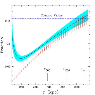
Figure 5.— Radial profiles of the baryon (solid black line, cyan $1\sigma$ error region) and gas (dotted red line, red $1\sigma$ error region) fractions of the fiducial hydrostatic model.

Table 3Gas and Baryon Fraction

	$f_{\rm gas,2500}$	$f_{\rm b,2500}$	$f_{\rm gas,500}$	$f_{\rm b,500}$	$f_{\rm gas,200}$	$f_{\rm b,200}$	$f_{\rm gas,vir}$	$f_{\rm b,vir}$
	$0.051\pm 0.001$	$0.072\pm 0.004$	$0.093\pm 0.003$	$0.104\pm 0.004$	$0.126\pm 0.007$	$0.134\pm 0.007$	$0.152\pm 0.010$	$0.159\pm 0.010$
(Max Like)	$(0.052)$	$(0.070)$	$(0.093)$	$(0.103)$	$(0.127)$	$(0.134)$	$(0.155)$	$(0.161)$
$M_{\rm stellar}^{\rm other}$	$\cdots$	+0.017	$\cdots$	+0.016	$\cdots$	+0.016	$\cdots$	+0.015
Spherical	$\cdots$	$\cdots$	${}_{-0.0009}^{+0.0006}$	$\cdots$	$\cdots$	$\cdots$	$\cdots$	$\cdots$
Einasto	$-0.001$	$0.000$	$-0.002$	$-0.001$	$-0.002$	$-0.001$	$-0.002$	$-0.001$
CORELOG	$0.003$	$0.002$	$-0.003$	$-0.001$	$-0.018$	$-0.015$	$-0.037$	$-0.035$
1 Break	$0.000$	$-0.000$	$-0.001$	$-0.001$	$-0.001$	$-0.001$	$-0.000$	$-0.000$
$\Lambda_{\nu}(T,Z)$	$0.000$	$0.001$	$0.004$	$0.004$	$0.010$	$0.010$	$0.015$	$0.016$
Response	$0.001$	$0.001$	$-0.001$	$-0.001$	$-0.003$	$-0.003$	$-0.004$	$-0.004$
Proj. Limit	${}^{+0.000}_{-0.000}$	${}^{+0.000}_{-0.000}$	${}^{+0.000}_{-0.000}$	${}^{+0.000}_{-0.000}$	${}^{+0.001}_{-0.000}$	${}^{+0.001}_{-0.000}$	${}^{+0.001}_{-0.000}$	${}^{+0.001}_{-0.000}$
SWCX	$-0.000$	$-0.000$	$-0.000$	$-0.000$	$-0.000$	$-0.000$	$-0.000$	$-0.000$
Distance	${}^{+0.002}_{-0.001}$	${}^{+0.001}_{-0.000}$	${}^{+0.002}_{-0.001}$	${}^{+0.002}_{-0.001}$	${}^{+0.003}_{-0.002}$	${}^{+0.003}_{-0.001}$	${}^{+0.003}_{-0.002}$	${}^{+0.002}_{-0.002}$
$N_{\rm H}$	$-0.000$	$0.000$	$0.001$	$0.001$	$0.002$	$0.002$	$0.003$	$0.004$
Fix $Z_{\rm Fe}(r_{\rm out})$	$0.000$	${}^{+0.001}_{-0.000}$	${}^{+0.003}_{-0.007}$	${}^{+0.003}_{-0.007}$	${}^{+0.006}_{-0.016}$	${}^{+0.006}_{-0.016}$	${}^{+0.009}_{-0.024}$	${}^{+0.009}_{-0.024}$
Solar Abun.	$-0.000$	$0.001$	$0.004$	$0.004$	$0.007$	$0.007$	$0.008$	$0.008$
PSF	$0.001$	$-0.000$	$-0.001$	$-0.002$	$-0.003$	$-0.003$	$-0.004$	$-0.004$
FI-BI	$0.002$	$0.001$	$0.003$	$0.003$	$0.005$	$0.005$	$0.007$	$0.007$
NXB	${}^{+0.001}_{-0.001}$	${}^{+0.001}_{-0.000}$	${}^{+0.002}_{-0.002}$	${}^{+0.001}_{-0.002}$	${}^{+0.001}_{-0.006}$	${}^{+0.001}_{-0.005}$	${}^{+0.000}_{-0.010}$	${}^{+0.000}_{-0.010}$
CXB	$-0.001$	$-0.000$	$-0.001$	$-0.001$	$-0.002$	$-0.002$	$-0.004$	$-0.004$
CXBSLOPE	${}^{+0.001}_{-0.001}$	${}^{+0.001}_{-0.001}$	${}^{+0.005}_{-0.009}$	${}^{+0.005}_{-0.008}$	${}^{+0.011}_{-0.018}$	${}^{+0.011}_{-0.018}$	${}^{+0.018}_{-0.027}$	${}^{+0.018}_{-0.027}$

The results for the baryon and gas fraction profiles using the fiducial hydrostatic model are displayed in Fig. 5, and the parameter constraints are listed in Table 3 including the systematic error budget. Similar to the results for the total mass, most of the systematic errors are insignificant in the sense that the estimated parameter changes in the gas and baryon fraction are comparable to or less than the $1\sigma$ statistical error. Again the most important changes occur for aspects of the background modeling (§6.6) and the treatment of the plasma emissivity (§6.8) and metal abundances (§6.5), particularly in the outermost apertures; i.e., the CXBSLOPE, $\Lambda_{\nu}(T,Z)$, Fix $Z_{\rm Fe}(r_{\rm out})$, and Solar Abun rows in Table 3. The CXBSLOPE and Fix $Z_{\rm Fe}(r)$ result in systematic errors almost $3\sigma$ in magnitude. (See §6 for a more detailed discussion of the systematic error budget.)

For most radii $f_{\rm b}<f_{\rm b,U}$, where $f_{\rm b,U}=0.155$ is the mean baryon fraction of the universe as determined by Planck (Planck Collaboration et al. 2014). Near $r_{108}$, $f_{\rm b}$ is consistent with $f_{\rm b,U}$, with the hot ICM consisting of 96% of the total baryons. These results are virtually identical to those for the Einasto model, where $f_{\rm b}=0.157\pm 0.011$ at $r_{108}$, whereas CORELOG has a smaller value, $f_{\rm b}=0.121\pm 0.008$

The preceding discussion considered the baryons contained in the hot ICM and stellar baryons associated only with the BCG as determined by the fitted $M_{\star}/L_{K}$. To estimate the stellar baryons from non-central cluster members and intracluster light (ICL) we follow the procedure we adopted in §4.3 of Humphrey et al. (2012a). Since the contribution of these non-BCG stellar baryons is not measured directly, we list it as a systematic error in Table 3 (see §6.2). At the largest radii these baryons are expected to increase the baryon fraction by $\sim 10\%,$ which is not much larger than the statistical error at $r_{108}.$

5.6. Mass and Density Slopes

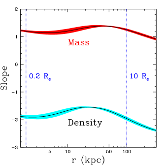
Figure 6.— Slopes (i.e., logarithmic derivatives) of the total mass and total mass density for the fiducial hydrostatic model. The error regions shown are $1\sigma$. The vertical lines indicate the regions between 0.2-10 stellar half-light radii $(R_{e})$ of the central galaxy that were studied in Humphrey & Buote (2010).

Table 4Mass-Weighted Total Density Slope

Radius	Radius
(kpc)	($R_{e}$)	$\langle\alpha\rangle$
4.9	0.5	$1.86\pm 0.07$
9.8	1.0	$1.80\pm 0.08$
19.7	2.0	$1.67\pm 0.07$
49.2	5.0	$1.62\pm 0.02$
98.3	10.0	$1.74\pm 0.04$

It is now well established that the total mass profiles of massive elliptical galaxies have density profiles very close to $\rho\sim r^{-\alpha}$ with $\alpha\approx 2$ over a wide range in radius. This relation extends to higher masses with smaller $\alpha$ in the central regions of clusters (e.g., Humphrey & Buote 2010; Newman et al. 2013b; Courteau et al. 2014; Cappellari et al. 2015, and references therein). In particular, in Humphrey & Buote (2010) it was shown that the total mass profiles inferred from hydrostatic studies of hot gas in massive elliptical galaxies, groups, and clusters, are fairly well-approximated by a single power-law over 0.2-10 stellar half-light radii $(R_{e})$ so that approximately, $\alpha=2.31-0.54\log(R_{e}/\rm kpc),$ a result consistent with that obtained from combination of stellar dynamics and strong gravitational lensing for massive elliptical galaxies (Auger et al. 2010).

In Fig. 6 we display the radial logarithmic derivatives (i.e., slopes) of the total mass and total density profiles for the fiducial hydrostatic model. The slopes are indeed slowly varying for our models, ranging from $\approx 1.2-1.4$ for the mass to $\approx$ -1.6 to -2.0 for the density over radii 0.2-10 $R_{e}$, representing a radial variation of $\pm 20\%$. In Table 4 we quote the mass-weighted total density slope $\langle\alpha\rangle$ following equation (2) of Dutton & Treu (2014),

$$\langle\alpha\rangle=3-\frac{d\ln M}{d\ln r},\hskip 11.38092pt\alpha\equiv-\frac{d\ln\rho}{d\ln r},$$ (4)

where $M$ is the total mass enclosed within radius $r$. Within $10R_{e}$, $\langle\alpha\rangle=1.74\pm 0.04$, which is consistent with the value of $\alpha=1.67^{+0.11}_{-0.10}$ we obtained previously from a power-law fit to the mass profile (Humphrey & Buote 2010) and with $\alpha=1.77$ obtained using the $\alpha-R_{e}$ scaling relation.

5.7. MOND

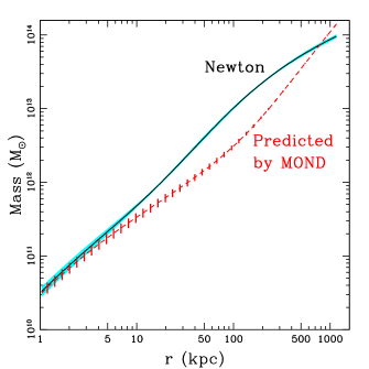
Figure 7.— (Left Panel) Radial profiles of the DM fraction for the fiducial hydrostatic model for the Newtonian (black and cyan) and MOND (red) cases. The shaded and hashed regions represent $1\sigma$ errors. (Right Panel) Newtonian mass profiles for (1) the total mass of the fiducial hydrostatic model (black and cyan, same as in Fig.4), and (2) the total mass profile predicted by MOND (red) from eqn. 6.

While the presence of dark matter is largely accepted by the astronomical community, it is worthwhile to examine interpretations of the observations that instead consider a modification of the gravitational force law. Here we consider the most widely investigated and successful modified gravity theory, MOND (Milgrom 1983), which nevertheless is unable to explain observations of galaxy clusters considering only the known baryonic matter (e.g., Sanders 1999; Pointecouteau & Silk 2005; Angus et al. 2008; Milgrom 2015). We investigate whether MOND can obviate the need for dark matter in RXJ 1159+5531 following the approach of Angus et al. (2008).

For an isolated spherical system the gravitational acceleration in Newton gravity, $g_{\rm N}=GM_{\rm N}(<r)/r^{2}$, and MOND, $g_{\rm M}=GM_{\rm M}(<r)/r^{2}$, have similar forms, where $M_{\rm N}(<r)$ and $M_{\rm M}(<r)$ are the respective enclosed masses within radius $r$. For some interpolating function, $\mu(g_{\rm N}/a_{0})$, the accelerations are related by, $g_{\rm M}=\mu(g_{\rm N}/a_{0})g_{\rm N}$, so that $M_{\rm M}=\mu(g_{\rm N}/a_{0})M_{\rm N}$, and $a_{0}\approx 1.2\times 10^{-8}$ cm s^-2 is the MOND acceleration constant. For $\mu(x)=x/(1+x)$, where $x=g_{\rm N}/a_{0}$, we have,

$$M_{\rm M}(<r)=\frac{M_{\rm N}(<r)}{1+a_{0}/g_{\rm N}(r)}.$$ (5)

In this way we easily compute the MONDian mass using the Newtonian mass we have derived previously; i.e., there is no different fitting required. Equation (5), being derived from the simple interpolating function $\mu$, has the undesirable property that $M_{\rm M}(<r)$ reaches a maximum value at some radius and then decreases (for more discussion of this point see Angus et al. 2008). Hence, for the moment we focus on results roughly within the radius where the MONDian mass reaches a maximum value.

In Fig. 7 for the fiducial hydrostatic model we compare the cumulative dark matter fractions $(M_{\rm DM}/M_{\rm total})$ inferred from Newtonian gravity and MOND. Like in the Newtonian case, MOND requires a dominant fraction of dark matter with increasing radius to match the X-ray data. At $r=100$ kpc the DM fraction is $85.0\pm 2.5\%$; i.e., the mass discrepancy is a factor of 6.7. Even when considering the contribution of baryons from (rather uncertain) non-central baryons (§6.2), the DM fraction is reduced by only a small amount to $\approx 82\%$.

It is also interesting to view the performance of MOND from a different perspective. Solving the MOND equation for $g_{\rm N}$ with the same interpolating function yields,

$$g_{\rm N}=\frac{g_{\rm M}}{2}\left(1+\sqrt{1+4\frac{a_{0}}{g_{\rm M}}}\,\,\,\,\right).$$ (6)

That is, given $g_{\rm M}$ evaluated using the baryonic mass profiles (i.e., stellar and gas) derived from the Newtonian analysis, this expression gives $g_{\rm N}$, and thus the Newtonian mass profile (with DM), that MOND would predict. In Fig. 7 we compare this “MOND predicted Newtonian mass profile” with the actual Newtonian total mass profile. The MOND profile under-predicts the Newtonian mass over most radii, with the largest deficit again occurring near $r=100$ kpc such that the predicted mass is $\approx 0.30M_{\rm N}$. The predicted profile crosses over the Newtonian profile shortly before $r_{200}$ and then exceeds the Newtonian profile afterwards.

In sum, consistent with previous results for X-ray groups and clusters, MOND requires a large fraction of dark matter similar to Newtonian gravity to explain the X-ray data.

5.8. Comparison to Previous Work

It is interesting to compare our results to those obtained by Humphrey et al. (2012a) who used only the Chandra data and the North Suzaku observation. Humphrey et al. (2012a) obtained best-fitting values, $M_{\star}/L_{K}=0.54$ (in solar units), $c_{\rm vir}=11.2$, $M_{\rm vir}=9.3\times 10^{13}\,M_{\odot}$, and $f_{\rm b,500}=0.124$ (includes non-BCG stellar baryons). All of these results agree within $1\sigma$ of the values obtained in our study (Tables 2 and 3).

The excellent agreement between the two studies is notable for several reasons. First, the addition of the Suzaku observations covering out to $r_{200}$ in the S, E, and W directions does not modify the results significantly, consistent with the results of Paper I indicating only small azimuthal variation in the ICM properties at large radius. Second, improved background modeling incorporating point sources resolved by offset Chandra observations – as well as improved calibration and data processing in the Chandra and Suzaku pipelines – do not change the results significantly. Finally, the consistent results between the studies provides a useful consistency check on the different implementations of the entropy-based hydrostatic modeling (e.g., treatment of self-gravity of gas mass, see §3) between the two studies using entirely different modeling software.

6. Error Budget

We have considered a variety of possible sources of systematic error and list a detailed error budget in Tables 2 and 3. Below we provide details on the construction of the error budgets.

6.1. Spherical Symmetry

Buote & Humphrey (2012b) showed that assuming a cluster is spherical when in fact it is ellipsoidal does not typically introduce large errors into the quantities inferred from hydrostatic modeling of the ICM. For a large range of intrinsic flattenings, they computed orientation-averaged biases (mean values and scatter) of several derived quantities, including halo concentration, total mass, and gas fraction.

We use the “NFW-EMD” results from Table 1 of Buote & Humphrey (2012b) to provide an estimate of the error arising from the assumption of spherical symmetry within $r_{500}$; i.e., the error from assuming the cluster is spherical when in fact it is a flattened ellipsoid viewed at a random orientation to the line of sight. From a study of cosmological dark matter halos Schneider et al. (2012) find that for a halo having mass similar to RXJ 1159+5531 the typical intrinsic short-to-long axis ratio is $\approx 0.5.$ We adopted this value for the error estimates on the concentration, mass, and gas fraction within $r_{500}$ in Tables 2 and 3 (“Spherical”) . In all cases the effect is insignificant.

6.2. Stellar Mass

While the BCG dominates the stellar mass in the central region of the cluster, smaller non-central galaxies and diffuse intracluster light (ICL) contribute significant stellar mass at larger radius. Due to the greater uncertainty of the amounts and distributions of these non-central baryons, we treat their contribution as a systematic effect to the baryon fraction. To account for these additional stellar baryons, we follow the procedure described in §4.3 of Humphrey et al. (2012a). For the non-central galaxies we use the result of Vikhlinin et al. (1999) that these galaxies comprise $\sim 25\%$ of the $V$-band stellar light. We assume this result also applies in the $K$ band with the same $M_{\star}/L_{K}$ as the BCG. Since we do not have a precise observational constraint on the ICL, we use the result from the theoretical study by Purcell et al. (2007) that the ICL contains up to $\sim 2$ times the stellar mass of the BCG and adopt this value to give a conservative reflection of the systematic error. We assume both components of non-central baryons are spatially distributed as the dark matter in our models.

The contribution of the non-central baryons to the baryon fraction are listed in Table 3 ($M_{\rm stellar}^{\rm other}$). These stellar baryons increase $f_{\rm b,vir}$ by $\sim 10\%$ to $0.174$ fully consistent with the value reported in Humphrey et al. (2012a) containing the contributions from both the BCG and non-central stellar baryons. This modified $f_{\rm b,vir}$ exceeds the cosmic value $f_{\rm b,U}=0.155$ by $2\sigma$ considering only the statistical error on our fiducial model, although the disagreement should be considered less significant given the uncertainties in the non-central stellar baryons.

6.3. Entropy Model

We examined the effect of restricting the entropy broken power-law model to only a single break (ONEBREAK). The effect is everywhere insignificant.

6.4. Dark Matter Model

The effects of using a DM profile different from NFW are indicated in the rows “Einasto” and “Corelog” in Tables 2 and 3. We have discussed the magnitudes of these systematic differences in §5.4 and §5.5.

6.5. Metal Abundances

We considered how choices made in the measurement of the metal abundances from the spectral fitting affected the results. (We refer the reader to Paper 1 for details on the spectral analysis.) First, we examined the impact of using different solar reference abundances. Whereas our default analysis used the solar abundance table of Asplund et al. (2006), the effect of instead using the tables of Anders & Grevesse (1989) or Lodders (2003) are listed in the “Solar Abun” row in Tables 2 and 3. The differences do not exceed the $1\sigma$ statistical error.

Second, since the spectra in the outermost apertures (i.e., at the virial radius) are the most background dominated and subject to systematic errors, we also examined the impact of fixing the metal abundance there at $0.1Z_{\odot}$ and $0.3Z_{\odot}$, bracketing the best-fitting value of $\sim 0.2Z_{\odot}$ (referred to as “$\Delta$abun” in Table 3 of Paper 1). As can be seen in the row “Fix $Z_{\rm Fe}(r_{\rm out})$” in Tables 2 and 3, this effect leads to one of the two largest systematic errors as mentioned above in §5.4 and §5.5.

6.6. Background

We considered the impacts of several choices made in the treatment of the background in the spectral fitting (see Paper 1). The effect of including a model for the solar wind charge exchange emission in the spectral analysis is listed in row “SWCX” in Tables 2 and 3. We find the effect to be insignificant in all cases.

To assess the sensitivity of the results to the particle background in the Suzaku observations, we artificially increased and decreased the estimated non-X–ray background component by $\pm 5\%$ and list the results in row “NXB” in Tables 2 and 3. In all instances the differences are insignificant for the stellar and total mass parameters. While this is also true at most radii for the gas and baryon fractions, at $r_{\rm vir}$ the differences are comparable to the $1\sigma$ error.

We also explored the sensitivity of our results to the extragalactic Cosmic X-ray Background (CXB) power-law component (see §5.1 of Paper 1). In Paper 1 by default we assumed a power-law component in our spectral fits with a slope fixed at $\Gamma=1.41$ (e.g., De Luca & Molendi 2004) and normalization free to vary. If we fix the normalization to the value expected for the cosmic average (see §2.3 of Paper 1), we obtain the results listed in row “CXB” in Tables 2 and 3. It is reassuring that the differences are all negligible. If instead we keep the normalization free to vary but change the slopes used to $\Gamma=1.3,1.5$ we obtain the results listed in row “CXBSLOPE” (corresponding to “CXB-$\Gamma$” in Table 3 of Paper 1). As already noted in §5.4 and §5.5, this effect leads to one of the two largest systematic errors. The differences are comparable to the $1\sigma$ errors within $r_{2500}$ and increase to 2-3$\sigma$ at $r_{\rm vir}$, where the data are most dominated by the background.

6.7. Miscellaneous Spectral Fitting

We performed other tests associated with the spectral fitting which we summarize here. In all cases they did not produce significant parameter differences in Tables 2 and 3. (1) The effect of varying the adopted value of Galactic $N_{\rm H}$ (Dickey & Lockman 1990) by $\pm 20\%$ is shown in row “$N_{\rm H}$” in Tables 2 and 3 (see §5.6 of Paper 1). (2) We varied the spectral mixing between extraction annuli by $\pm 5\%$ from our default case to assess the impact of small changes on how we account for the large, energy-dependent Suzaku PSF (see §5.3 of Paper 1). The results are given in row “PSF” in Tables 2 and 3. (3) By default we allowed the normalization of the ICM model for annuli on the Suzaku XIS front-illuminated (FI) and back-illuminated (BI) chips to be varied separately to allow for any calibration differences. To assess the impact of this choice, we also performed the spectral fitting requiring the same normalizations for the FI and BI chips (§5.7 of Paper 1) and the results are given in the row “FI-BI” in Tables 2 and 3.

6.8. Miscellaneous Hydrostatic Modeling

Here we describe a few remaining tests we performed associated with choices made in our hydrostatic modeling procedure. First, we varied the cluster redshift by $\pm 5\%$ in our hydrostatic models (it was similarly varied in the spectral fitting in Paper 1), and the results are listed in row “Distance” of Tables 2 and 3. The differences are everywhere insignificant. Second, we explored the impact of changing the default bounding radius of the cluster model. Whereas the default employed is 2.5 Mpc, in row “Proj. Limit” of Tables 2 and 3 we show the differences resulting from instead using either 2.0 Mpc or 3.0 Mpc for the bounding radius. In all cases the effect is negligible. Next we examined the sensitivity of the results to the “response weighting” (§3) by instead performing no such weighting. As indicated in row “Response” of Tables 2 and 3 the differences are insignificant.

Finally, we examined how our choices regarding the modeling of the plasma emissivity affect the results. As discussed in §3, the hydrostatic models by default take the measured metal abundance profile in projection and assigns it to be the true three-dimensional profile which is then used (along with the temperature) to compute the plasma emissivity $\Lambda_{\nu}(T,Z)$. Our default procedure to do this assignment uses the Chandra data and only the N Suzaku observation. We investigated using instead each of the other three Suzaku pointings. For a more rigorous test, we also fitted a projected, emission-weighted parametric model to the projected iron abundance profile (Fig. 13 of Paper 1). We employed a multi-component model consisting of two power-laws mediated by an exponential (eqn. 5 of Gastaldello et al. 2007) and a constant floor of $0.05Z_{\odot}$. The results of both of these tests for the plasma emissivity are listed in row “$\Lambda_{\nu}(T,Z)$” of Tables 2 and 3. The differences are among the largest, though in most cases are less than the $1\sigma$ error. In detail, both the metallicity model test and the cases where the E and S Suzaku pointings are used produce negligible results. The differences indicated in the tables are largest when the W Suzaku pointing is used to assign the metallicity profile.

7. Discussion

7.1. Distinct Stellar BCG and DM Halo Components

Previously in Zappacosta et al. (2006) we made the observation that in massive galaxy clusters (i.e., with virial mass larger than a few $10^{14}\,M_{\odot}$) the total gravitating mass profile inferred from X-ray studies is itself generally well-described by a single NFW profile without any need for a distinct component for stellar mass from the central BCG. On the other hand, individual massive elliptical galaxies (e.g., Humphrey et al. 2006, 2011, 2012b) and group-scale systems (e.g., Gastaldello et al. 2007; Zhang et al. 2007; Démoclès et al. 2010; Su et al. 2014) with virial masses less than $10^{14}\,M_{\odot}$ studied with X-rays usually (but do not always) require distinct stellar BCG and DM mass components.

The most massive clusters where X-ray observations clearly require distinct stellar BCG (with a reasonable stellar mass-to-light ratio) and DM (without an anomalously low concentration) mass components are RXJ 1159+5531 ($M_{200}=7.9\pm 0.6\times 10^{13}\,M_{\odot}$) and A262 ($M_{200}=9.3\pm 0.8\times 10^{13}\,M_{\odot}$, Gastaldello et al. 2007). Hence, from the perspective of X-ray studies, $\sim 10^{14}\,M_{\odot}$ appears to represent a point of demarcation above which the total mass profile, rather than the DM profile, is represented by a single NFW component.

Since X-ray images of the central regions of cool core clusters typically display irregular features (e.g., cavities) believed to be associated with intermittent AGN feedback, it is tempting to speculate that the inability to detect a distinct stellar BCG component in massive cool core clusters reflects simply a strong violation of the approximation of hydrostatic equilibrium used to measure the mass profile. However, Newman and colleagues (Newman et al. 2013b) have used a combination of stellar dynamics and gravitational lensing to perform detailed studies of the radial mass profiles in several galaxy clusters. In their most recent study of 10 clusters (Newman et al. 2015), they also propose $\sim 10^{14}\,M_{\odot}$ as the mass above which the total mass profile, rather than the DM, is well-described by a single NFW component.

The consistent picture obtained by X-ray, stellar dynamics, and lensing studies provides strong evidence for the reality of this transition mass. This has important implications for models of cluster formation since $\sim 10^{14}\,M_{\odot}$ appears to represent the mass scale where dissipative processes become important in the formation of the central regions of galaxy groups and clusters; i.e., above this mass the impact of dissipative processes on the total mass profile has been counteracted by late-time collisionless merging that re-establishes the NFW profile (e.g., Loeb & Peebles 2003; Laporte & White 2015).

As discussed in §5.6, the various mass components of RXJ 1159+5531 combine to produce a nearly power-law total mass profile with slowly varying logarithmic density slope ranging between $\alpha\approx-1.6$ to -2.0 within a radius $\sim 100$ kpc ($\sim 10R_{e}$). This result is not strongly dependent on the assumed DM profile (NFW, Einasto, CORELOG). The slope $\alpha$ is consistent with that inferred from the scaling relation with $R_{e}$ proposed by Humphrey & Buote (2010) and Auger et al. (2010).

This nearly power-law behavior in the total mass obeying scaling relations between $\alpha$ and $R_{e}$ (and stellar density) for early-type galaxies is known as the “Bulge-Halo Conspiracy.” Using empirically constrained $\Lambda$CDM models Dutton & Treu (2014) argue that a complex balance between feedback and baryonic cooling is required to explain this “conspiracy.”

7.2. High DM Concentration

While some early X-ray studies indicated that fossil groups and clusters have unusually large NFW DM concentrations, essentially all of those measurements were inflated by neglecting to include the stellar BCG component in the mass modeling (e.g., Mamon & Łokas 2005). For the fossil cluster RX J1416.4+2315, Khosroshahi et al. (2006) accounted for the presence of the stellar BCG component and inferred a DM concentration of $c_{200}=11.2\pm 4.5$ which is about $2\sigma$ above the value of $\sim 4$ expected for a relaxed halo with $M_{200}=3.1\times 10^{14}\,M_{\odot}$ according to Dutton & Macciò (2014). The result we obtained for RXJ 1159+5531 in §5.4 is a $3\sigma$ discrepancy, providing even stronger evidence for an above-average concentration in a fossil cluster, suggestive of a halo that formed earlier than the general population. (We note that we have not included adiabatic contraction (e.g., Blumenthal et al. 1986; Gnedin et al. 2004) of the DM halo in our model which would lead to an even larger concentration.) We caution, however, that as noted in §5.4, when the Einasto DM model is employed the significance of RXJ 1159+5531 as an outlier is somewhat reduced.

It is also worth emphasizing that from the perspective of relaxed, low-redshift X-ray clusters, the concentration of RXJ 1159+5531 is not very remarkable. The only study that has measured the X-ray concentration-mass relation for a sizable number of relaxed systems having masses both lower and higher than RXJ 1159+5531 is Buote et al. (2007), which also included the measurement of RXJ 1159+5531 by Gastaldello et al. (2007). Our value for RXJ 1159+5531 is only $\sim 1\sigma$ larger than the mean relation obtained by Buote et al. (2007). The higher normalization of the X-ray concentration-mass relation can be explained by including reasonable star formation and feedback in the cluster simulations (Rasia et al. 2013) which are not present in the DM-only simulations of Dutton & Macciò (2014).

7.3. Gas Fraction

Recently, Eckert et al. (2015) have used gas masses inferred from XMM-Newton and total masses from weak lensing to measure gas fractions at $r_{500}$ for a large cluster sample. They conclude that the gas fractions measured in this way are significantly smaller than those obtained from hydrostatic studies (e.g., Ettori 2015). By assuming the weak lensing masses are accurate, Eckert et al. (2015) infer a hydrostatic mass bias of $0.72^{+0.08}_{-0.07}$. When compared to numerical hydrodynamical simulations (Le Brun et al. 2014), the small gas fractions obtained by Eckert et al. (2015) favor an extreme feedback model in which a substantial amount of baryons are ejected from cluster cores.

From our hydrostatic analysis of RXJ 1159+5531 we measured within a radius $r_{500}$: $M_{500}=(5.9\pm 0.4)\times 10^{13}\,M_{\odot}$ and $f_{\rm gas}=0.093\pm 0.003$ (Tables 2 and 3). For this value of $M_{500}$, the best-fitting relation for the gas fraction obtained by Eckert et al. (2015) gives $f_{\rm gas}=0.05$ implying a hydrostatic mass bias of $\approx 80\%$. Since the wealth of evidence indicates the ICM in RXJ 1159+5531 is very relaxed (see below in §7.4), including that the value of $f_{\rm gas}\approx 0.09$ we measure agrees much better with the cluster gas fractions produced in the simulations of Le Brun et al. (2014) considering plausible cooling and supernova feedback, we do not believe such a large hydrostatic mass bias in RXJ 1159+5531 is supported by the present observations. Instead, we believe these results for RXJ 1159+5531 support the suggestion by Eckert et al. (2015) that the weak lensing masses are biased high.

7.4. Hydrostatic Equilibrium Approximation

As we have noted previously in the related context of elliptical galaxies (see §8.2.2.1 of Buote & Humphrey 2012a), even without possessing direct, precise measurements of the hot gas kinematics, it is still possible to identify relaxed systems where the hydrostatic equilibrium approximation should be most accurate. RXJ 1159+5531 is a cool core cluster and displays a very regular X-ray image from the smallest scales probed by Chandra (with little or no evidence for AGN-induced disturbances) out to $r_{200}$. The Suzaku images mapping the radial region from $\sim r_{2500}-r_{200}$ with full azimuthal coverage display remarkably homogeneous ICM properties (Paper 1).

We are able to obtain a good representation of the X-ray data with hydrostatic models with reasonable values for the model parameters: (1) the stellar mass-to-light ratio is consistent with stellar population synthesis models (§5.4); (2) the value of the concentration, while statistically higher than the expected mean of the halo population, is within the $2\sigma$ cosmological intrinsic scatter (§5.4), and, at any rate, deviations from hydrostatic equilibrium due to additional non-thermal pressure support should tend to produce anomalously low, not high, concentrations by leading to smaller inferences of the virial mass and radius (e.g., see discussion in §6.2 of Buote et al. 2007); and (3) the baryon fraction is consistent with the cosmic value.

Although it is tempting to ascribe the very relaxed state of RXJ 1159+5531 to it being a fossil cluster, recent evidence suggests that the X-ray properties of fossil systems are not significantly distinguishable from the general cluster population (Girardi et al. 2014). The apparently highly relaxed ICM within $r_{200}$ implies that non-thermal pressure support is small throughout the cluster and, as such, constrains theories that predict a large amount of non-thermal pressure support from the magneto-thermal instability (MTI) in the ICM outside of $r_{500}$ (e.g., Parrish et al. 2012).

8. Conclusions

We present a detailed hydrostatic analysis of the ICM of the fossil cluster, RXJ 1159+5531, a system especially well-suited for study of its mass distribution with current X-ray observations. At a redshift of 0.081 it is sufficiently distant to allow mapping of its entire virial region on the sky with reasonable exposures, while still being close enough to spatially resolve the central regions near the BCG. Previous studies have shown this cluster to have a remarkably regular and undisturbed ICM (Vikhlinin et al. 1999, 2006; Gastaldello et al. 2007; Humphrey et al. 2012a). In Paper 1 we presented three new Suzaku observations in the South, East, and West directions, which, in conjunction with the existing Suzaku pointing to the North and central Chandra data, allow complete azimuthal and radial coverage on the sky within $r_{200}$. Our separate analysis of the ICM in each of the four directions found the ICM properties to be very homogenous in azimuth, testifying to the relaxed state of the ICM out to $r_{200}$ (see Paper 1).

We constructed hydrostatic models and fitted them simultaneously to the projected ICM temperature and emission measure ($\propto\rho_{gas}^{2}$) measured individually for each Chandra and Suzaku observation (see Paper 1). We employ an “entropy-based” procedure (Humphrey et al. 2008; Buote & Humphrey 2012a) where the hydrostatic equilibrium equation is expressed in terms of the entropy proxy $S$ and total mass, which allows the additional contraint of convective stability ($dS/dr>0$) to be easily enforced. Our fiducial model consists of a power-law with two breaks and a constant for $S$, a Sersic model for the stellar mass of the BCG, and an NFW DM halo. We explore the parameter space and determine confidence limits using a Bayesian Monte Carlo procedure and find the fiducial model is a good fit to the data.

We constructed a detailed budget of systematic errors (§6) to assess the impact that different data analysis and modeling choices have on our measurements. The largest systematic effects are associated with the background spectral models, metal abundances, and modeling the plasma emissivity variation with radius. These effects are most significant at the largest radii, although none of them change qualitatively the results of the fiducial model.

The principal results are the following:

• Entropy The radial entropy profile of the ICM is described well by the power-law model with either one or two breaks. When rescaled in terms of the “virial” entropy $(S_{500})$, the entropy exceeds the $\sim r^{1.1}$ profile predicted by pure gravitational formation until $\sim r_{200}$, but does not fall below it at any radius. Further rescaling of the entropy by $(f_{\rm gas}/f_{b,U})^{2/3}$ matches very well the $\sim r^{1.1}$ profile, suggesting that feedback has spatially redistributed the ICM rather than raised its temperature (Pratt et al. 2010).

• Pressure The radial pressure profile expressed in terms of $P_{500}$ slightly exceeds the mean“universal” pressure profile of Arnaud et al. (2010), but is consistent within the scatter of that profile.

• BCG Stellar Mass & Dissipation Scale The stellar mass of the BCG is clearly required by the model fits and yields a $K$-band stellar mass-to-light ratio, $M_{\star}/L_{K}=0.61\pm 0.11\,M_{\odot}/L_{\odot}$, consistent with stellar population synthesis models for a Milky-Way IMF. This makes RXJ 1159+5531 along with A262 (Gastaldello et al. 2007) the most massive clusters where X-ray studies have measured such a distinct BCG stellar component and supports recent work (Newman et al. 2015; Laporte & White 2015) suggesting that $\sim 10^{14}\,M_{\odot}$ represents the mass scale above which dissipation does not dominate the formation of the inner regions of clusters (§7.1).

• Dark Matter Profiles Despite the high-quality X-ray data covering the entire region within $r_{200}$, our model fits do not statistically distinguish between NFW, Einasto $(n=5)$, or CORELOG (singular isothermal sphere with a core) profiles for the DM halo. This contrasts with clusters much more massive than RXJ 1159+5531 where previous X-ray studies (e.g. Pointecouteau et al. 2005) clearly disfavor pseudo-isothermal models in favor of NFW, which is also found by recent results from the CLASH survey from gravitational lensing analysis of several very massive clusters (Umetsu et al. 2015). Allowing the Einasto index $n$ to be free does not improve the fit significantly and yields, $n=5.8^{+4.6}_{-2.0}$ or $\alpha=1/n=0.17^{+0.09}_{-0.08}$, very consistent with the values expected for a DM halo of the mass of RXJ 1159+5531 (Dutton & Macciò 2014).

• High Concentration For the fiducial model (i.e., with an NFW profile) we obtain $c_{200}=8.4\pm 1.0$ and $M_{200}=(7.9\pm 0.6)\times 10^{13}\,M_{\odot}$. The concentration exceeds the value of 5.2 expected for the mean relaxed cluster population in the Planck cosmology (Dutton & Macciò 2014) by $3\sigma$. It is also a $\sim 2\sigma$ outlier considering the intrinsic scatter of the theoretical relation, although the discrepancy is reduced to a little more than a $1\sigma$ outlier when the Einasto DM profile is used. These properties make RXJ 1159+5531 the most significant over-concentrated fossil cluster to date (see §7.2), indicating an earlier formation time than the average cluster at its redshift. However, with respect to a sample of relaxed, low-redshift galaxy systems studied in X-rays spanning a mass range of $\sim 10^{12}-10^{15}\,M_{\odot}$, the concentration of RXJ 1159+5531 is only $\sim 1\sigma$ above the mean relation of Buote et al. (2007).

• Gas and Baryon Fraction Considering only the baryons associated with the ICM and the BCG, we obtain a baryon fraction at $r_{200}$, $f_{\rm b,200}=0.134\pm 0.007$, that is slightly below the Planck value (0.155) for the universe, but the baryon fraction continues to rise with radius so that, $f_{\rm b,vir}=0.159\pm 0.010$ at $r_{\rm vir}=r_{108}$. Taking into account estimates for the stellar baryons associated with non-central galaxies and intracluster light (ICL) increases these values by $\approx 0.015$, in which case $f_{\rm b,vir}$ marginally exceeds (by $2\sigma$) the cosmic value. Since our estimate of the ICL mass is very uncertain, we do not consider the disagreement to be significant; i.e., the baryon fraction is consistent with the cosmic value and therefore no significant baryon loss from the system.

• Slope of the Total Mass Profile The total mass profile is nearly a power-law over radii $0.2-10R_{e}$ with a slope ranging from $\approx 1.2-1.4$ and density slope $\alpha$ ranging from -1.6 to -2.0. Within $10R_{e}$, the mass-weighted slope of the total density profile, $\langle\alpha\rangle=1.74\pm 0.04$, is consistent with the value $\alpha=1.77$ obtained using the $\alpha-R_{e}$ scaling relation (Humphrey & Buote 2010; Auger et al. 2010).

• MOND Following the procedure of Angus et al. (2008) using a particular simple interpolating function $\mu(g_{\rm N}/a_{0})$, we computed mass profiles in the context of MOND. We find that MOND requires DM fractions nearly as large as for conventional Newton gravity: At $r=100$ kpc the DM fraction is $85.0\%\pm 2.5\%$ implying a mass discrepancy of a factor of 6.7. The DM fraction decreases to $\approx 82\%$ considering the (rather uncertain) contribution of non-central stellar baryons (§6.2). Therefore, consistent with previous results for other X-ray groups and clusters, MOND requires a large DM fraction to explain the X-ray data.

In sum, our hydrostatic analysis of the ICM emission within $r_{200}$ yields baryon and DM properties quite consistent with typical clusters for its virial mass in the $\Lambda$CDM paradigm. The only notable exception is the higher-than-average NFW concentration parameter that, nevertheless, is not unreasonable for a fossil system expected to form earlier than the general cluster population. Hence, RXJ 1159+5531 appears to be an optimal, benchmark cluster for hydrostatic studies of its ICM.

References

- Allen et al. (2011) Allen, S. W., Evrard, A. E., & Mantz, A. B. 2011, ARA&A, 49, 409
- Anders & Grevesse (1989) Anders, E., & Grevesse, N. 1989, Geochim. Cosmochim. Acta, 53, 197
- Angus et al. (2008) Angus, G. W., Famaey, B., & Buote, D. A. 2008, MNRAS, 387, 1470
- Arnaud (1996) Arnaud, K. A. 1996, in Astronomical Society of the Pacific Conference Series, Vol. 101, Astronomical Data Analysis Software and Systems V, ed. G. H. Jacoby & J. Barnes, 17
- Arnaud et al. (2010) Arnaud, M., Pratt, G. W., Piffaretti, R., et al. 2010, A&A, 517, A92
- Asplund et al. (2006) Asplund, M., Grevesse, N., & Jacques Sauval, A. 2006, Nuclear Physics A, 777, 1
- Auger et al. (2010) Auger, M. W., Treu, T., Bolton, A. S., et al. 2010, ApJ, 724, 511
- Bell et al. (2003) Bell, E. F., McIntosh, D. H., Katz, N., & Weinberg, M. D. 2003, ApJS, 149, 289
- Blumenthal et al. (1986) Blumenthal, G. R., Faber, S. M., Flores, R., & Primack, J. R. 1986, ApJ, 301, 27
- Buote (2000a) Buote, D. A. 2000a, ApJ, 539, 172
- Buote (2000b) —. 2000b, MNRAS, 311, 176
- Buote et al. (2007) Buote, D. A., Gastaldello, F., Humphrey, P. J., et al. 2007, ApJ, 664, 123
- Buote & Humphrey (2012a) Buote, D. A., & Humphrey, P. J. 2012a, in Astrophysics and Space Science Library, Vol. 378, Astrophysics and Space Science Library, ed. D.-W. Kim & S. Pellegrini, 235
- Buote & Humphrey (2012b) Buote, D. A., & Humphrey, P. J. 2012b, MNRAS, 421, 1399
- Bykov et al. (2015) Bykov, A. M., Churazov, E. M., Ferrari, C., et al. 2015, Space Sci. Rev., 188, 141
- Cappellari et al. (2015) Cappellari, M., Romanowsky, A. J., Brodie, J. P., et al. 2015, ApJ, 804, L21
- Chabrier (2003) Chabrier, G. 2003, ApJ, 586, L133
- Conroy & van Dokkum (2012) Conroy, C., & van Dokkum, P. G. 2012, ApJ, 760, 71
- Courteau et al. (2014) Courteau, S., Cappellari, M., de Jong, R. S., et al. 2014, Reviews of Modern Physics, 86, 47
- De Luca & Molendi (2004) De Luca, A., & Molendi, S. 2004, A&A, 419, 837
- Démoclès et al. (2010) Démoclès, J., Pratt, G. W., Pierini, D., et al. 2010, A&A, 517, A52
- Dickey & Lockman (1990) Dickey, J. M., & Lockman, F. J. 1990, ARA&A, 28, 215
- Dutton & Macciò (2014) Dutton, A. A., & Macciò, A. V. 2014, MNRAS, 441, 3359
- Dutton & Treu (2014) Dutton, A. A., & Treu, T. 2014, MNRAS, 438, 3594
- Eckert et al. (2015) Eckert, D., Ettori, S., Coupon, J., et al. 2015, ArXiv e-prints, arXiv:1512.03814
- Einasto (1965) Einasto, J. 1965, Trudy Astrofizicheskogo Instituta Alma-Ata, 5, 87
- Ettori (2015) Ettori, S. 2015, MNRAS, 446, 2629
- Ettori et al. (2013) Ettori, S., Donnarumma, A., Pointecouteau, E., et al. 2013, Space Sci. Rev., 177, 119
- Feroz et al. (2009) Feroz, F., Hobson, M. P., & Bridges, M. 2009, MNRAS, 398, 1601
- Gastaldello et al. (2007) Gastaldello, F., Buote, D. A., Humphrey, P. J., et al. 2007, ApJ, 669, 158
- Girardi et al. (2014) Girardi, M., Aguerri, J. A. L., De Grandi, S., et al. 2014, A&A, 565, A115
- Gnedin et al. (2004) Gnedin, O. Y., Kravtsov, A. V., Klypin, A. A., & Nagai, D. 2004, ApJ, 616, 16
- Humphrey & Buote (2010) Humphrey, P. J., & Buote, D. A. 2010, MNRAS, 403, 2143
- Humphrey et al. (2012a) Humphrey, P. J., Buote, D. A., Brighenti, F., et al. 2012a, ApJ, 748, 11
- Humphrey et al. (2008) Humphrey, P. J., Buote, D. A., Brighenti, F., Gebhardt, K., & Mathews, W. G. 2008, ApJ, 683, 161
- Humphrey et al. (2009) —. 2009, ApJ, 703, 1257
- Humphrey et al. (2011) Humphrey, P. J., Buote, D. A., Canizares, C. R., Fabian, A. C., & Miller, J. M. 2011, ApJ, 729, 53
- Humphrey et al. (2006) Humphrey, P. J., Buote, D. A., Gastaldello, F., et al. 2006, ApJ, 646, 899
- Humphrey et al. (2012b) Humphrey, P. J., Buote, D. A., O’Sullivan, E., & Ponman, T. J. 2012b, ApJ, 755, 166
- Jarrett et al. (2000) Jarrett, T. H., Chester, T., Cutri, R., et al. 2000, AJ, 119, 2498
- Khosroshahi et al. (2006) Khosroshahi, H. G., Maughan, B. J., Ponman, T. J., & Jones, L. R. 2006, MNRAS, 369, 1211
- Kitayama et al. (2014) Kitayama, T., Bautz, M., Markevitch, M., et al. 2014, ArXiv e-prints, arXiv:1412.1176
- Kravtsov & Borgani (2012) Kravtsov, A. V., & Borgani, S. 2012, ARA&A, 50, 353
- Laporte & White (2015) Laporte, C. F. P., & White, S. D. M. 2015, MNRAS, 451, 1177
- Le Brun et al. (2014) Le Brun, A. M. C., McCarthy, I. G., Schaye, J., & Ponman, T. J. 2014, MNRAS, 441, 1270
- Lodders (2003) Lodders, K. 2003, ApJ, 591, 1220
- Loeb & Peebles (2003) Loeb, A., & Peebles, P. J. E. 2003, ApJ, 589, 29
- Mamon & Łokas (2005) Mamon, G. A., & Łokas, E. L. 2005, MNRAS, 362, 95
- Mazzotta et al. (2004) Mazzotta, P., Rasia, E., Moscardini, L., & Tormen, G. 2004, MNRAS, 354, 10
- McLaughlin (1999) McLaughlin, D. E. 1999, AJ, 117, 2398
- Merritt et al. (2006) Merritt, D., Graham, A. W., Moore, B., Diemand, J., & Terzić, B. 2006, AJ, 132, 2685
- Milgrom (1983) Milgrom, M. 1983, ApJ, 270, 365
- Milgrom (2015) —. 2015, MNRAS, 454, 3810
- Nagai et al. (2007) Nagai, D., Vikhlinin, A., & Kravtsov, A. V. 2007, ApJ, 655, 98
- Navarro et al. (1997) Navarro, J. F., Frenk, C. S., & White, S. D. M. 1997, ApJ, 490, 493
- Newman et al. (2015) Newman, A. B., Ellis, R. S., & Treu, T. 2015, ArXiv e-prints, arXiv:1503.05282
- Newman et al. (2013a) Newman, A. B., Treu, T., Ellis, R. S., & Sand, D. J. 2013a, ApJ, 765, 25
- Newman et al. (2013b) Newman, A. B., Treu, T., Ellis, R. S., et al. 2013b, ApJ, 765, 24
- Nulsen & Bohringer (1995) Nulsen, P. E. J., & Bohringer, H. 1995, MNRAS, 274, 1093
- Parrish et al. (2012) Parrish, I. J., McCourt, M., Quataert, E., & Sharma, P. 2012, MNRAS, 419, L29
- Planck Collaboration et al. (2014) Planck Collaboration, Ade, P. A. R., Aghanim, N., et al. 2014, A&A, 571, A16
- Pointecouteau et al. (2005) Pointecouteau, E., Arnaud, M., & Pratt, G. W. 2005, A&A, 435, 1
- Pointecouteau & Silk (2005) Pointecouteau, E., & Silk, J. 2005, MNRAS, 364, 654
- Pratt et al. (2010) Pratt, G. W., Arnaud, M., Piffaretti, R., et al. 2010, A&A, 511, A85
- Purcell et al. (2007) Purcell, C. W., Bullock, J. S., & Zentner, A. R. 2007, ApJ, 666, 20
- Rasia et al. (2013) Rasia, E., Borgani, S., Ettori, S., Mazzotta, P., & Meneghetti, M. 2013, ApJ, 776, 39
- Rasia et al. (2004) Rasia, E., Tormen, G., & Moscardini, L. 2004, MNRAS, 351, 237
- Reiprich et al. (2013) Reiprich, T. H., Basu, K., Ettori, S., et al. 2013, Space Sci. Rev., 177, 195
- Retana-Montenegro et al. (2012) Retana-Montenegro, E., van Hese, E., Gentile, G., Baes, M., & Frutos-Alfaro, F. 2012, A&A, 540, A70
- Sanders (1999) Sanders, R. H. 1999, ApJ, 512, L23
- Sarazin (1986) Sarazin, C. L. 1986, Reviews of Modern Physics, 58, 1
- Schneider et al. (2012) Schneider, M. D., Frenk, C. S., & Cole, S. 2012, J. Cosmology Astropart. Phys, 5, 030
- Smith et al. (2015) Smith, R. J., Lucey, J. R., & Conroy, C. 2015, MNRAS, 449, 3441
- Su et al. (2015) Su, Y., Buote, D., Gastaldello, F., & Brighenti, F. 2015, ApJ, 805, 104
- Su et al. (2014) Su, Y., Gu, L., White, III, R. E., & Irwin, J. 2014, ApJ, 786, 152
- Tozzi & Norman (2001) Tozzi, P., & Norman, C. 2001, ApJ, 546, 63
- Umetsu et al. (2015) Umetsu, K., Zitrin, A., Gruen, D., et al. 2015, ArXiv e-prints, arXiv:1507.04385
- Vikhlinin et al. (2006) Vikhlinin, A., Kravtsov, A., Forman, W., et al. 2006, ApJ, 640, 691
- Vikhlinin et al. (1999) Vikhlinin, A., McNamara, B. R., Hornstrup, A., et al. 1999, ApJ, 520, L1
- Voit et al. (2005) Voit, G. M., Kay, S. T., & Bryan, G. L. 2005, MNRAS, 364, 909
- Zappacosta et al. (2006) Zappacosta, L., Buote, D. A., Gastaldello, F., et al. 2006, ApJ, 650, 777
- Zhang et al. (2007) Zhang, Z., Xu, H., Wang, Y., et al. 2007, ApJ, 656, 805
- Zibetti et al. (2009) Zibetti, S., Charlot, S., & Rix, H.-W. 2009, MNRAS, 400, 1181