Variational Monte Carlo method for the Baeriswyl wavefunction: application to the one-dimensional bosonic Hubbard model

Abstract

A variational Monte Carlo method for bosonic lattice models is introduced. The method is based on the Baeriswyl projected wavefunction. The Baeriswyl wavefunction consists of a kinetic energy based projection applied to the wavefunction at infinite interaction, and is related to the shadow wavefunction already used in the study of continuous models of bosons. The wavefunction at infinite interaction, and the projector, are represented in coordinate space, leading to an expression for expectation values which can be evaluated via Monte Carlo sampling. We calculate the phase diagram and other properties of the bosonic Hubbard model. The calculated phase diagram is in excellent agreement with known quantum Monte Carlo results. We also analyze correlation functions.

I Introduction

Variational Monte Carlo is a powerful tool to calculate the properties of quantum systems. In general, expectation values of physical quantities over conveniently chosen variational wavefunctions allow the application of Monte Carlo sampling methods. For fermionic lattice models, commonly used variational wavefunctions are the Gutzwiller Gutzwiller63 ; Gutzwiller65 and Baeriswyl Baeriswyl86 ; Baeriswyl00 ; Dzierzawa97 wavefunctions (GWF and BWF, respectively). The GWF starts with a non-interacting wavefunction, and projects out configurations according to the interaction. For fermionic systems, evaluation of physical quantities can be done approximately via a combinatorial approximation, or exactly in the case of the one-dimensional Metzner87 ; Metzner89 and the infinite Metzner88 ; Metzner89 ; Metzner90 dimensional case. In between those two cases the state-of-the-art is the Monte Carlo method developed by Yokoyama and Shiba Yokoyama87a ; Yokoyama87b . For bosonic systems, the GWF reduces to mean-field theory Rokhsar91 .

The BWF can be considered the counterpart of the GWF: the starting point is the wavefunction with inifinite interaction, and the projection applied thereonto is a function of the hopping energy. For fermionic systems this wavefunction already has a history Baeriswyl86 ; Baeriswyl00 ; Dzierzawa97 ; Hetenyi10 ; Dora16 . For a model of interacting spinless fermions the BWF produces excellent results for the ground state energy Dora16 . We note also, that a method known as the momentum dependent local ansatz, in which momentum dependent amplitudes of pairs are used as variational parameters, was recently developed Patoary13a ; Patoary13b ; Kakehashi14 . While there are a number of schemes to solve the BWF for fermionic systems, it has, to the best of our knowledge, not been applied to bosonic systems.

In this work we develop a variational Monte Carlo (VMC) method for correlated bosonic models based on the BWF and apply it to the bosonic Hubbard model Gersch63 ; Fisher89 (BHM) with on-site interaction. The BHM was originally proposed to study actual materials (bosons in porous materials), but they were recently also realized experimentally as ultra-cold gases in optical lattices Jaksch98 ; Greiner02 . The BHM has been treated by analytical and numerical means, including mean-field theory Fisher89 ; Rokhsar91 , perturbative expansion Freericks96 , quantum Monte Carlo (QMC) Batrouni90 ; Krauth91 ; Scalettar05 ; Rousseau06 ; Kashurnikov96b ; Rombouts06 , density matrix renormalization group (DMRG) Kuhner00 ; Ejima11 ; Zakrzewski08 ; Carrasquilla13 ; Kuhner98 , and exact diagonalization (ED)  Kashurnikov96a . DMRG is limited to one dimension, QMC is limited to small system sizes, and ED is limited to even smaller system sizes. Our variational Monte Carlo approach is shown to give good quantitative results, at the same time, it is not restricted to one dimension, and is less computationally demanding than QMC or ED. It can also be generalized to more complex bosonic strongly correlated models with distance dependent interaction, and/or disorder.

We calculate some of the properties of the BHM. As expected, the ground state energy obtained using our VMC method has a lower value than the one given by mean-field theory. More importantly, for the phase diagram, our results are in excellent quantitative agreement with the quantum Monte Carlo results of Rousseau et al. Rousseau06 ; Rousseau08a ; Rousseau08b . We also obtain the Kosterlitz-Thouless point at the tip of the Mott lobes, and find that our calculations underestimate the values calculated by others Kuhner00 ; Ejima11 ; Zakrzewski08 ; Kashurnikov96a ; Kashurnikov96b ; Rombouts06 . We also calculate the one-particle reduced density matrix at integer and away from integer fillings. For integer fillings we find decay to zero. The decay is well approximated by an exponential function, implying the absende of a condensate.

The rest of this paper is organized as follows. In the following section we describe in detail the variational Monte Carlo method and our implementation of it for the BHM. In section III we present our results for the phase diagram and one-body density matrix. Subsequently, we conclude our work.

II Model and method

II.1 Bosonic Hubbard model and the Baeriswyl variational wavefunction

We study the BHM with nearest neighbor hopping in one dimension at fixed particle number. The Hamiltonian is

$$H=-J\sum_{x=1}^{L}\left(\hat{c}^{\dagger}_{x+1}\hat{c}_{x}+\hat{c}^{\dagger}_{x}\hat{c}_{x+1}\right)+U\sum_{x=1}^{L}\hat{n}_{x}(\hat{n}_{x}-1),$$ (1)

where $L$ denotes the number of sites, $J$ and $U$ are the hopping and interaction parameters, respectively. The BWF has the form

$$|\Psi_{B}\rangle=\exp(-\alpha\hat{T})|\Psi_{\infty}\rangle,$$ (2)

where $\alpha$ denotes the variational parameter, and $|\Psi_{\infty}\rangle$ is the wavefunction at $U=\infty$. $\hat{T}$ denotes the hopping operator (first term in Eq. (1)). The idea of the Baeriswyl wavefunction is to start with the infinitely interacting wavefunction, and act on it with a projector which implements hoppings.

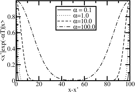
Figure 1: Kinetic energy propagator as a function of distance for different values of $\alpha$.

II.2 Variational Monte Carlo

The expectation value of an operator $\hat{O}$ can be written as

$$\langle\hat{O}\rangle=\langle\Psi_{B}|\hat{O}|\Psi_{B}\rangle=\frac{\langle\Psi_{\infty}|e^{-\alpha\hat{T}}\hat{O}e^{-\alpha\hat{T}}|\Psi_{\infty}\rangle}{\langle\Psi_{\infty}|e^{-2\alpha\hat{T}}|\Psi_{\infty}\rangle}.$$ (3)

The following derivations will treat a one particle system, but they are generally applicable. We also assume that the operator $\hat{O}$ is diagonal in the coordinate representation. Inserting coordinate identities, $\sum_{x}|x\rangle\langle x|=1,$ results in

$$\langle\hat{O}\rangle=\sum_{x_{L}}\sum_{x_{C}}\sum_{x_{R}}P(x_{L},x_{C},x_{R})O(x_{C}),$$ (4)

where the probability distribution $P(x_{L},x_{C},x_{R})$ is

$$P(x_{L},x_{C},x_{R})=\frac{1}{\Omega}\langle\Psi_{\infty}|x_{L}\rangle K(x_{L},x_{C})K(x_{C},x_{R})\langle x_{R}|\Psi_{\infty}\rangle,$$ (5)

where

$$K(x,x^{\prime})=\langle x|\exp(-\alpha\hat{T})|x^{\prime}\rangle$$ (6)

with $\Omega$ the normalization determined by the requirement that

$$\sum_{x_{L},x_{C},x_{R}}P(x_{L},x_{C},x_{R})=1.$$ (7)

The quantum particle is represented by three coordinates which we call the “left”, “center”, and “right” coordinates. Operators diagonal in the coordinate representation can be evaluated using the center coordinate. In quantum Monte Carlo based methods whether finite temperature Pollet12 ; Ceperley95 or ground state Baroni99 ; Hetenyi99 ; Sarsa00 each particle is represented by a large number of coordinates (Trotter slices) whose number must be increased for accurate results as the temperature is lowered. Therefore, while our method is not exact as the QMC is, it is significantly less demanding of computational resources. Within our VMC method we can reach larger system sizes. In this work, we limit ourselves to system sizes with $L=50,100$, in order to have a direct reliable comparison to the available QMC results.

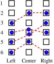
Figure 2: (Color online) Representation of our variational algorithm. In our method there are three replicas of the system, labelled left, center, and right. The black squares represent the lattice sites of the one-dimensional system for each such replica. The blue filled circles represent particles. Each particle is represented by one replica on the left, center, and right lattices. The dashed red line represents the kinetic energy projection operator (Eq. (8)). The left and right replicas correspond to the infinitely interacting system. Since in the case there would be an infinite energy cost, there are no sites with more than one particle among the left and right replicas. In the center replica of the lattice, two or more particles can be on the same lattice.

The kinetic energy projection operator can be expressed as

$$K(x,x^{\prime})=\frac{1}{L}\sum_{k}\exp[-\alpha\epsilon_{k}+ik(x-x^{\prime})],$$ (8)

and is shown in Fig. 1. As $\alpha$ increases the propagator also increases in value, allowing for delocalization through increased quantum fluctuations. Given that $P(x_{L},x_{C},x_{R})$ is positive and normalized, MC techniques can be applied to evaluate expectation values. In the continuum limit, the kinetic energy propagator reads $K(r)=I_{r}(2\alpha J)$ where $I_{n}(x)$ are the modified Bessel functions of the first kind.

The kinetic energy can be evaluated by constructing an estimator based on taking the logarithmic derivative of the quantity $\Omega$ with respect to the variational parameter $\alpha$. We can write the normalization as

$$\Omega=\langle\Psi_{\infty}|\exp(-2\alpha\hat{T})|\Psi_{\infty}\rangle,$$ (9)

and the average kinetic energy as

$$\langle T\rangle=-\frac{1}{2\Omega}\frac{\partial\Omega}{\partial\alpha}.$$ (10)

Writing $\Omega$ in terms of the projected wavefunction one can show that

$$\langle T\rangle=\sum_{x_{L},x_{C},x_{R}}P(x_{L},x_{C},x_{R})T(x_{L},x_{C},x_{R}),$$ (11)

where

$$T(x_{L},x_{C},x_{R})=-\frac{1}{2}\left[\frac{\partial\ln K(x_{L},x_{C})}{\partial\alpha}+\frac{\partial\ln K(x_{C},x_{R})}{\partial\alpha}\right].$$ (12)

The generalization to the many-body case is straightforward, but it is in order to make some comments. A typical configuration is represented in Fig. 2. In that figure a lattice of $6$ sites is shown. The left, center, and right replicas of the lattice are all represented. A single quantum particle is represented by three classical particles, one on each lattice replica. The dashed lines on the figure connecting the three particles refer to the kinetic energy projector $K(x,x^{\prime})$ (Eq. (8)). Since the left and right coordinates refer to the infinite interaction wavefunction ($\Psi_{\infty}$) no configuration occurs in which more than one particle is on a particular lattice site. This will be the case for fillings less than one. In general for a filling of $n$ the left and right replicas will only have lattice sites with int($n$) or int($n$)$+1$ particles. However, in the center replica, the lattice sites with any number of particles can occur, since the projector does not place any restrictions there. Since the casting of our method above is in terms of first quantization, exchange is implemented by explicit exchange moves of pairs of particles on the left or right lattices. One randomly chooses a pair and then propose the exchange as a Monte Carlo move. This is similar to how it is done in the continuous quantum Monte Carlo methods, such as path-integral Monte Carlo Ceperley95 .

II.3 One-particle reduced density matrix

A quantity of general interest is the one-particle reduced density matrix (RDM). The RDM gives information about Bose-Einstein condensation Penrose56 : if it tends to a finite value at long distance, a condensate is present in the system. The RDM (in our case for the BWF) is given by

$$\rho(y,x)=\langle\Psi_{B}|\hat{c}_{y}^{\dagger}\hat{c}_{x}|\Psi_{B}\rangle.$$ (13)

The difficulty with calculating this quantity stems from the fact that it is not diagonal in the coordinate representation. While this is also true for the kinetic energy, there only nearest-neighbor hoppings contribute, moreover, one can simply take the derivative with respect to the variational parameter.

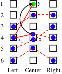
Figure 3: (Color online) Representation of a configuration with virtual hopping which contributes to the one-particle reduced density matrix (Eq. (13)). The virtual hopping takes place from site $y$ to site $x$, indicated by the black semi-circular arrow. The contribution to the average reduced density matrix is the proportion of the Baeriswyl propagators denoted by the straight solid red lines (see also Eq. (14)). The propagators connect the left coordinate of the particle considered (in this case site $4$) to the central coordinate after virtual hopping (in this case site $1$, particle represented by green circle), and the propagator between the left coordinate to the unmoved central coordinate of the particle (site $4$, particle represented by blue circle).

In the context of our variational method, the operator $\hat{c}_{x}^{\dagger}\hat{c}_{y}$ corresponds to a virtual hopping from $y$ to $x$, and has the effect of giving rise to virtual configurations in which a given particle has two central coordinates. One of these is located at $x$, the other at $y$. One of these ($x$) is connected to the left coordinate of the given particle via a Baeriswyl projector, the other ($y$) to the right coordinate. To calculate $\rho(x,y)$ one starts with a regular configuration, obtained from the Monte Carlo sampling outlined above. One choses a particle (say, with coordinates $x_{L}$, $x$, $x_{R}$, with $x$ denoting the central coordinate) and calculates the ratio

$$\gamma=\frac{K(x_{L},y)}{K(x_{L},x)}.$$ (14)

Part of $\rho(x,y)$ is the average of contributions of this type. The scenario for calculating such contributions to the RDM is visually represented in Fig. 3. The two Baeriswyl projectors in the expression in Eq. (14) are shown in the figure by the solid straight lines. For integer fillings, averaging over configurations of this type is all that is needed.

In general, there is another class of virtual configurations which needs to be considered. Away from integer filling, there are holes among the left and right coordinates. As such, the virtual hopping to which $\hat{c}_{x}^{\dagger}\hat{c}_{y}$ coordsponds can also move either the left or the right coordinate. In Fig. 4 this state of affairs is represented. In this case the quantity which must be considered is

$$\gamma=\frac{K(y_{L},y)}{K(x_{L},x)},$$ (15)

where $y_{L}$ represents the site to which $x_{L}$ is moved. In the original configuration, from which this virtual configuration is sampled, this site is an empty site (or for fillings $n>1$, they are sites with int($n$) number of particles, rather than int($n$)+1).

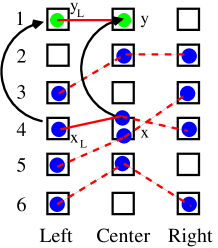
Figure 4: (Color online) Representation of a configuration with virtual hopping which contributes to the one-particle reduced density matrix (Eq. (13)). The virtual hopping takes place from site $y$ to site $x$, indicated by the black semi-circular arrow. At the same time, a virtual hopping takes place among the left coordinates, also indicated by a black semi-circular arrow. The contribution to the average reduced density matrix is the proportion of the Baeriswyl propagators denoted by the straight solid red lines (see also Eq. (15)). The propagators connect left coordinate of the particle (site $1$, particle represented by green circle) to the central coordinate of the particle (site $1$, particle represented by green circle), both after the virtual hopping, and the propagator left coordinate (site $4$, represented by a blue circle) and the central coordinate of the particle (site $4$, represented by a blue circle) both before the virtual hopping.

II.4 Relation to shadow wavefunction

The BWF is the lattice analog of the shadow wavefunction (SWF) Reatto88 ; Vitiello88 , used often in continuous systems in the study of supersolidity. To show this, we consider a one-dimensional system with Hamiltonian

$$H=-\frac{\hbar^{2}}{2m}\frac{\partial^{2}}{\partial x^{2}}+V(x).$$ (16)

In one dimension the SWF is given by

$$\Psi(x)=\phi_{1}(x)\int dx^{\prime}f(|x-x^{\prime}|)\phi_{2}(x^{\prime}).$$ (17)

The function $\phi_{1}(x)$ is a real-space projection operator (for now we will take it to be one). The term $f(|x-x^{\prime}|)$ is chosen Reatto88 ; Vitiello88 to be a Gaussian therefore we can write

$$\Psi(x)=A\int dx^{\prime}\exp[-C(x-x^{\prime})^{2}]\phi_{2}(x^{\prime}),$$ (18)

where $A$ is the normalization and $C$ is the variational constant.

Let us now start with a wavefunction of the form

$$\exp(-\alpha\hat{T})|\phi_{2}\rangle=\int dx^{\prime}\exp(\alpha\hat{T})|x^{\prime}\rangle\langle x^{\prime}|\phi_{2}\rangle,$$ (19)

in which the kinetic energy propagator is applied to the state $\phi_{2}$. Inserting a momentum identity, and casting the function in the coordinate representation, results in

$$\langle x|\exp(-\alpha\hat{T})|\phi_{2}\rangle=\sqrt{\frac{m}{2\alpha\pi}}$$ (20)

$$\times\int dx^{\prime}\exp\left(-\frac{m}{2\alpha}(x-x^{\prime})^{2}\right)\phi_{2}(x^{\prime}).$$

The constant $C$ is identified as $C=\frac{m}{2\alpha}$. The other real-space projection $\phi_{1}(x)$ can be implemented also in the case of a lattice, this would be an example of a Gutzwiller-Baeriswyl projected wavefunction Baeriswyl00 ).

II.5 Implementation

Before MC sampling the kinetic energy propagator, as well as the estimator, is calculated (Fig. (1)) and stored. We apply two types of MC moves. We move the left, central, and right coordinates by standard Metropolis sampling from the distribution $P(x_{L},x_{C},x_{R})$. We also use exchange moves: two left (or right) particles are randomly chosen and exchanged. These moves are essential for simulating a bosonic system. The calculations below show results from runs on the order of $10^{6}$ MC steps. The number of independent data points are on the order of $10^{5}$. In our energy calculations error bars typically occurred in the fourth digit of the kinetic or potential energies.

Figure 5: (Color online) Energy per lattice site for fillings of one and one-half calculated by our variational Monte Carlo method, and mean-field theory. Lines with symbols represent variational Monte Carlo calculations, lines without symbols are the results of mean-field theory.

III Results

Figure 6: Phase diagram of the bosonic Hubbard model according to the Baeriswyl wavefunction (full circles connected by solid line) compared to quantum Monte Carlo Results of Rousseau et al. Rousseau06 (open diamonds) recalculated via QMC Rousseau08a ; Rousseau08b . $n$ denotes the filling factor. The error bars in the calculations are smaller than the thickness of the symbols.

For a system of $L=100$ sites we calculated the hopping and the potential term. The energy was minimized for different values of $J/U$. The total energy as a function of $J/U$ for $100$ and $50$ particles based on our variational calculations is shown in Fig. 5. Also shown are results for the same quantity from mean-field theory. As is well-known, the mean-field theory of the Bose-Hubbard model Fisher89 give equations in which the chemical potential is held fixed and the particles fluctuate. We solve the usual mean-field equations for a given $J/U$ adjusting the chemical potential to correspond to an average filling of one and one-half. The figure shows results for the total energy without the term proportional to the chemical potential (in order to compare the corresponding quantities from both calculations). The mean-field energies are quite close to the variational Monte Carlo results, but the variational Monte Carlo results are always below the mean-field theory. For small $J/U$ the energy of the system with filling one is larger than the energy for half-filling, but this changes between $J/U=0.4$ and $J/U=0.5$.

The mean-field results indicate a phase transition at fixed filling. At a filling of one the phase transition occurs at $J/U\approx 0.172$, and it can be seen in a discontinuous change in the slope of the energy and the order parameter Fisher89 . In our variational calculations no discontinuity in the slope of the energy is found, although gap closure does occur (discussed below). This result is qualitatively similar to what happens when the BWF is applied to fermions: there also, no metal-insulator transition is found Dzierzawa97 at fixed filling. The curves of the calculated phase diagram (Fig. 6) arise purely as a result of a phase transition which occurs when the particle number is changed; away from integer fillings the phase is superfluid.

To calculate the phase diagram we follow the same procedure, as well as the same parametrization, as Scalettar et al. Scalettar05 and Rousseau et al. Rousseau06 . Using the definition of the chemical potential $\mu=E(N+1)-E(N)$ we obtain a density vs. chemical potential curve. The curve exhibits plateaus at integer fillings (similar to Fig. 2 of Ref. Scalettar05 ). From the edges of the plateaus the phase diagram can be constructed. The results are shown in Fig. 6. Inspite of being a variational method, the results are in good quantitative agreement with the quantum Monte Carlo simulations (c.f. Fig. 11 in Ref. Rousseau06 ). Also, for larger values of $J$ than shown in the figure the gap closes indicating a superfluid phase.

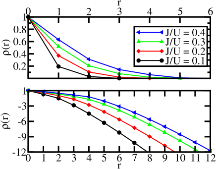
Figure 7: (Color online) One-particle reduced density matrix for systems at filling one with $J/U=0.1,0.2,0.3,0.4$. The bottom panel is a semi-log plot. The bottom panel is a semilog plot, the $y$-axis is labelled according to powers of ten. The decay of the one-body reduced density matrices is nearly exponential, implying the absence of a condensate.

At the tip of the Mott lobe, at integer filling when $J/U$ is varied a transition is known to occur. From scaling theory it is known to belong to the Kosterlitz-Thouless universality class Fisher89 . The point at which this phase transition occurs can be estimated from inspecting the gap (it closes at the transition point), but since small errors make a big difference at the tip, it can also be obtained Kuhner00 from the expression for the gap

$$\Delta(J)=A\exp\left(-\frac{B}{\sqrt{J_{KT}-J}}\right).$$ (21)

Our results also indicate gap closure. For a system with $L=200$ lattice sites we obtain $J_{KT}=0.4604(2)$ from fitting this function to our data for $J>2$, and $J_{KT}\approx 0.46$ by calculating the point where the gap closes.

The estimates given by our method significantly underestimate the Kosterlitz-Thouless point $J_{KT}$ compared to other results in the literature Factor2 . DMRG calculations of Kühner et al. Kuhner00 find $J_{KT}=0.594(2)$, those of Ejima et al. Ejima11 find $J_{KT}=0.610(2)$, Zakrzewski and Delande Zakrzewski08 find $J_{KT}=0.5950\pm 0.020$ for the first Mott lobe, and $J_{KT}=0.350\pm 0.004$ for the second one. An exact diagonalization study of Kashurnikov and Svistunov Kashurnikov96a gives $J_{KT}=0.608(4)$, QMC studies find $J_{KT}=0.600\pm 0.010$ Kashurnikov96b and $J_{KT}=0.610(8)$ Rombouts06 . We attribute the discrepancy between the above results and ours to the limitation of the BWF in describing the behavior of the system as $J$ increases. By construction, the BWF is expected Baeriswyl86 ; Baeriswyl00 to produce reliable results for small hoppings.

We also calculated the RDM for several cases. Fig. 7 shows the results of our calculations for a system of $L=100$ at filling one for different values of $J/U$. The functions show decay, although there is some deviation from the expected exponential decay (exponential decay implies the absence of a condensate). Our estimates for the correlation lengths $\xi$ for the different cases are: $\xi=0.605(5),0.95(3),1.31(5),1.66(8)$, for $J/U=0.1,0.2,0.3,0.4$, respectively. These results were obtained from fitting a simple exponential function to the calculated RDMs. We emphasize that the exponential functions fit our correlation functions significantly better than power law decay, as expected.

We have also calculated the RDM for systems away from integer fillings. We used a system of size $L=50$, with particle numbers $N=49$ and $N=48$. In this case, the decay does not reach zero, in other words, a finite condensate fraction is found, which is unexpected in one dimension. We emphasize that our variational approach has certain limitations which are likely the cause of this behavior. On one hand, our $U=\infty$ function is represented in a purely combinatorial manner, neglecting correlations between holes or extra particles when near integer filling. This approximation is correct in infinite dimensions. Apart from this, as in the original shadow wavefunction, a spatially dependent (Gutzwiller) projector could be added to act on the central coordinate, an approach which would improve how correlations are captured. This would correspond to the so-called Baeriswyl-Gutzwiller wavefunction.

IV Conclusion

We developed a variational Monte Carlo method for strongly correlated bosonic systems based on the Baeriswyl wavefunction. Our method was applied to the simple bosonic Hubbard model in one dimension, but it can be generalized to more complex models (e.g., long-range interaction, disorder), and can be applied in any number of dimensions. We calculated the phase diagram of the Bose-Hubbard model, and found excellent agreement with results from quantum Monte Carlo simulations. Our calculations recover the shape of the Mott lobes well. The tip of the Mott lobes is underestimated. We also calculated the one-particle reduced density matrix. At a filling of one we see decay which is nearly exponential.

References

- (1) M. C. Gutzwiller, Phys. Rev. Lett., 10 159 (1963).
- (2) M. C. Gutzwiller, Phys. Rev., 137 A1726 (1965).
- (3) D. Baeriswyl in Nonlinearity in Condensed Matter, Ed. A. R. Bishop, D. K. Campbell, D. Kumar, and S. E. Trullinger, Springer-Verlag (1986).
- (4) D. Baeriswyl, Found. Physics, 30 2033 (2000).
- (5) M. Dzierzawa, D. Baeriswyl, and L. M. Martelo, Helv. Phys. Acta, 70 124 (1997).
- (6) W. Metzner and D. Vollhardt: Phys. Rev. Lett., 59 (1987) 121.
- (7) W. Metzner and D. Vollhardt: Phys. Rev. Lett., 62 (1989) 324.
- (8) W. Metzner and D. Vollhardt: Phys. Rev. B, 37 (1988) 7382.
- (9) W. Metzner and D. Vollhardt: Helv. Phys. Acta, 63 (1990) 364.
- (10) H. Yokoyama and H. Shiba, J. Phys. Soc. Jpn., 56 1490 (1987).
- (11) H. Yokoyama and H. Shiba, J. Phys. Soc. Jpn., 56 3582 (1987).
- (12) D. S. Rokhsar and B. G. Kotliar Phys. Rev. B, 44 10328 (1991).
- (13) B. Hetényi, Phys. Rev. B, 82 115104 (2010).
- (14) B. Dóra, M. Haque, F. Pollmann and B. Hetényi , Phys. Rev. B, 93 115124 (2016).
- (15) M. A. R. Patoary, S. Chandra, and Y. Kakehashi, J. Phys. Soc. Jpn. 82 013701 (2013).
- (16) M. A. R. Patoary and Y. Kakehashi, J. Phys. Soc. Jpn. 82 084710 (2013).
- (17) Y. Kakehashi, S. Chandra, D. Rowlands, M. A. R. Patoary Mod. Phys. Lett. 28 1430007 (2014).
- (18) H. Gersch and G. Knollmann Phys. Rev., 129 959 (1963).
- (19) M. P. A. Fisher, P. B. Weichman, G. Grinstein, and D. S. Fisher, Phys. Rev. B, 40 546 (1989).
- (20) D. Jaksch, C. Bruder, J. I. Cirac, C. W. Gardiner, P. Zoller, Phys. Rev. Lett., 81 3108 (1998).
- (21) M. Greiner, O. Mandel, T. Esslinger, T. W. Hänsch, I. Bloch, Nature, 415 39 (2002).
- (22) J. K. Freericks and H. Monien Phys. Rev. B, 53 2691 (1996).
- (23) G.G. Batrouni, R. T. Scalettar, and G. T. Zimányi, Phys. Rev. Lett., 65 1765 (1990).
- (24) W. Krauth, and N. Trivedi, Europhys. Lett. 14 627 (1991).
- (25) R. T. Scalettar, G. Batrouni, P.J.H. Denteneer, F. Hébert, A. Muramatsu, M. Rigol, V. G. Rousseau et M. Troyer, J. Low Temp. Phys., 140 315 (2005).
- (26) V. G. Rousseau, D. P. Arovas, M. Rigol, F. Hébert, G. G. Batrouni, and R. T. Scalettar, Phys. Rev. B, 73 174516 (2006).
- (27) V. A. Kashurnikov, A. V. Kravasin, B. V. Svistunov, JETP Lett. 64 99 (1996).
- (28) S. M. A. Rombouts, K. Van Houcke, and L. Pollet, Phys. Rev. Lett. 96 180603 (2006).
- (29) T. D. Kühner, S. R. White, and H. Monien, Phys. Rev. B, 61 12474 (2000).
- (30) S. Ejima, H. Fehske, and F. Gebhard, EPL 93 30002 (2011).
- (31) J. Zakrzewski and D. Delande, AIP Conf. Proc. 1076 292 (2008).
- (32) J. Carrasquilla, S. R. Manmana, and M. Rigol, Phys. Rev. A 87 043606 (2013).
- (33) T. D. Kühner, and H. Monien, Phys. Rev. B, 58 R14741 (1998).
- (34) V. A. Kashurnikov and B. V. Svistunov, Phys. Rev. B 53 11776 (1996).
- (35) V. G. Rousseau, Phys. Rev. E, 77 056705 (2008).
- (36) V. G. Rousseau, Phys. Rev. E, 78 056707 (2008).
- (37) L. Pollet, Rep. Prog. Phys., 75 094501 (2012).
- (38) D. M. Ceperley Rev. Mod. Phys., 67 279 (1995).
- (39) S. Baroni and S. Moroni, Phys. Rev. Lett., 82 4745 (1999).
- (40) B. Hetényi, E. Rabani, and B. J. Berne, J. Chem. Phys., 110 6143 (1999).
- (41) A. Sarsa, K. E. Schmidt, and R. W. Magro, J. Chem. Phys., 113 1366 (1999).
- (42) O. Penrose and L. Onsager, Phys. Rev. 104 576 (1956).
- (43) L. Reatto and G. L. Masserini, Phys. Rev. B, 38 4516 (1988)
- (44) S. Vitiello, K. Runge, and M. H. Kalos, Phys. Rev. Lett., 60 1970 (1988).
- (45) The results reported here for comparison are based on a different definition of the Bose-Hubbard model, in which the potential is divided by two. For this reason, the results reported in the original papers are half of the values cited here. ——————