How Much Cache is Needed to Achieve Linear Capacity Scaling in Backhaul-Limited Dense Wireless Networks?

Abstract

Dense wireless networks are a promising solution to meet the huge capacity demand in 5G wireless systems. However, there are two implementation issues, namely the interference and backhaul issues. To resolve these issues, we propose a novel network architecture called the backhaul-limited cached dense wireless network (C-DWN), where a physical layer (PHY) caching scheme is employed at the base stations (BSs) but only a fraction of the BSs have wired payload backhauls. The PHY caching can replace the role of wired backhauls to achieve both the cache-induced MIMO cooperation gain and cache-assisted Multihopping gain. Two fundamental questions are addressed. Can we exploit the PHY caching to achieve linear capacity scaling with limited payload backhauls? If so, how much cache is needed? We show that the capacity of the backhaul-limited C-DWN indeed scales linearly with the number of BSs if the BS cache size is larger than a threshold that depends on the content popularity. We also quantify the throughput gain due to cache-induced MIMO cooperation over conventional caching schemes (which exploit purely the cached-assisted multihopping). Interestingly, the minimum BS cache size needed to achieve a significant cache-induced MIMO cooperation gain is the same as that needed to achieve the linear capacity scaling.

I Introduction

In dense wireless networks, the dense BS deployment brings the network closer to mobile users and thus can significantly improve spectral efficiency per unit area. For instance, the capacity of dense wireless networks scales linearly with the number of BSs $N$ if all BSs are equipped with wired payload backhauls. However, there are also two key technical challenges: the interference and the backhaul cost issues.

Compared to traditional cellular networks, the interference in dense wireless networks is more severe due to the increased BS density. Recently, some advanced interference mitigation schemes such as cooperative MIMO (Co-MIMO) [1, 2, 3] have been proposed. By sharing both channel state information (CSI) and payload data among the concerned BSs, the Co-MIMO can transform the wireless network from an unfavorable interference topology to a favorable broadcast topology, where the interference can be mitigated much more efficiently. However, the Co-MIMO technique requires high capacity backhaul for payload exchange between BSs, which is a cost bottleneck in dense wireless networks.

Moreover, a dense wireless network with all small BSs having wired payload backhauls suffers from high CAPEX and OPEX [4]. To address this issue, a more flexible backhaul solution has been proposed where only a fraction of $N_{0}\ll N$ BSs have wired payload backhauls, and the other BSs are connected to the core network via low-cost wireless backhauls [5, 6, 7, 8]. However, in this case, the performance is limited by the number of wired payload backhauls $N_{0}$ and the total network capacity can only scale as $\Theta\left(N_{0}\right)$.

This paper addresses the following fundamental questions in dense wireless networks. Can we realize the benefit of MIMO cooperation without wired backhaul connections between the BSs? Can we achieve linear capacity scaling with only $N_{0}\ll N$ wired payload backhauls? According to classical information theory, where the information is considered as random raw bits, the answers to these questions are negative. However, in practice, we are more concerned about delivering content. By exploiting the fact that content is “cachable”, we show that the answers to both questions can be positive using PHY caching at the BSs. Specifically, there are two fundamental benefits associated with PHY caching in dense wireless networks. If the content accessed by users exists simultaneously at the BS caches, the BSs can engage in Co-MIMO and enjoy a large MIMO cooperation gain, as illustrated in Fig. 1 for the red and green data flows. This is referred to as cache-induced opportunistic Co-MIMO. If the content requested by a user is distributed in the caches of the nearby BSs, this user can directly obtain the requested content from the nearby BSs, which reduces the number of hops from the source BSs to the destination user, as illustrated in Fig. 1 for the purple data flow. This is referred to as cache-assisted multihopping.

We are interested in studying the fundamental linear capacity scaling in the backhaul-limited C-DWN and how to exploit the above benefits of PHY caching to achieve the linear capacity scaling. Some related works are reviewed below.

Capacity scaling law in wireless ad hoc networks: The capacity scaling law of wireless ad hoc networks was first studied by Gupta and Kumar in the seminal paper [9], where they showed that in a large wireless ad hoc networks with $N$ random located nodes, the aggregate throughput of classical multihop communication scheme scales at most as $\Theta\left(\sqrt{N}\right)$. After that, a number of works [10, 11, 12] have studied the information theoretic capacity scaling law under different channel models and traffic models. Specifically, it was shown in [13] that under a physical channel model with the path loss exponent $\alpha\in\left(2,3\right]$, the total network capacity scales as $\Theta\left(N^{2-\alpha/2}\right)$, which can approach the linear capacity scaling law $\Theta\left(N\right)$ as $\alpha$ approaches $2$. However, this capacity gain is at the cost of increased system complexity due to the complicated hierarchical MIMO cooperation [13, 14]. In [14], the authors studied the capacity scaling in ad hoc networks with arbitrary node placement. The capacity regions of the ad hoc network with more complicated unicast or multicast traffic model have been studied in [15].

Capacity scaling law in cellular networks: Unlike ad hoc networks, cellular networks consist of infrastructure gateways as the sources of data traffics. When all BSs have wired payload backhauls, the capacity scales linearly with the number of the BSs. However, adding more backhaul-connected BSs (i.e., BSs that have wired backhauls) leads to high CAPEX and OPEX [4]. A more cost-effective way to enhance the capacity is to add relay nodes to enable multihop communications between the users and BSs. It was shown in [16] that multihop cellular networks with $N$ relay nodes and $M$ BSs achieve higher per-node throughput than pure cellular networks (with only $M$ BSs) by a scaling factor of $\log_{2}N$. However, the total capacity order $\Theta\left(M\log_{2}N\right)$ is still far from the linear capacity $\Theta\left(N\right)$ for large $N$.

Wireless Caching: Recently, wireless caching has been proposed as a cost-effective solution to handle the high traffic rate caused by content delivery applications [17, 5]. For example, [18] proposed coded caching schemes that can create coded multicast opportunities. A proactive caching paradigm was proposed in [19] to exploit both the spatial and social structure of the wireless networks. The fundamental tradeoff in wireless D2D caching networks have also been studied in [20, 21, 22, 23]. Furthermore, [24] studied the joint optimization of cache content replication and routing in a regular network and identified the throughput scaling laws for various regimes. Note that although both [24] and this paper focus on the scaling law of cached wireless networks, they are different in many aspects. First, the throughput scaling law in [24] is obtained by assuming a specific caching and multihop transmission scheme. On the other hand, the capacity scaling law studied in this paper is an information theoretic scaling law which does not depend on any specific caching or PHY transmission scheme. Second, the role of caching is also different. In [24], the main role of caching is to reduce the number of hops in multihop transmissions. In this paper, the role of PHY caching includes both the cache-assisted multihopping and the cache-induced MIMO cooperation. Third, the network topologies are also different. [24] considered a regular network where all nodes are placed on a perfect grid and have homogeneous traffic. This paper considers a general network with arbitrary node placements and content requests. Finally, the key difference between wireless and wired networks is that the performance of wireless networks is fundamentally limited by the interference due to the broadcast nature of wireless channel. However, this unique feature of wireless networks and the associated PHY transmission scheme are not considered in the analysis in [24]. In this paper, we consider joint design of PHY caching and transmission schemes (e.g., the PHY transmission modes in our design depend on the cache mode of the requested file) where interference plays a vital role (e.g., both frequency partitioning and cache-induced MIMO cooperation are proposed to mitigate the interference).

The above works on wireless caching do not consider cache-induced MIMO cooperation among the BSs. The concept of cached-induced opportunistic Co-MIMO was first introduced in [25, 26]. The achievable throughput scaling laws of ad hoc networks with PHY caching were also studied in [27]. However, the capacity scaling in the backhaul-limited C-DWN and the corresponding order-optimal PHY caching and transmission schemes have not been addressed in the literature. This paper provides solutions to the following important questions associated with the backhaul-limited C-DWN.

• How much cache is needed to achieve the linear capacity scaling in the backhaul-limited C-DWN? We show that the total network capacity of the backhaul-limited C-DWN scales as $\Theta\left(N\right)$ when the BS cache size is larger than a threshold that depends on the content popularity distribution. We quantify the minimum BS cache size required to achieve the linear capacity scaling as a function of the content popularity parameter.

• What is the order-optimal capacity achieving scheme? We propose an order-optimal achievable scheme, which can exploit both the cache-induced opportunistic Co-MIMO and cache-assisted multihopping to achieve the linear capacity scaling for the backhaul-limited C-DWN.

• What is the role of cache-induced Co-MIMO? Exploiting cache-induced Co-MIMO cannot change the throughput scaling law of the backhaul limited C-DWN. However, it helps to mitigate the interference and increase the spatial degrees of freedom (i.e., the number of data streams that can be simultaneously transmitted) in the backhaul limited C-DWN. As a result, a huge throughput gain can be achieved by exploiting cache-induced Co-MIMO. In this paper, we derive closed-form expression for this cache-induced MIMO cooperation gain and analyze the minimum BS cache size needed to achieve a significant cache-induced MIMO cooperation gain.

The rest of the paper is organized as follows. In Section II, we introduce the system model. In Section III, we give some preliminary results on capacity bound in backhaul-limited dense wireless networks without cache. In Section IV, we present the main results on the linear capacity scaling law in the backhaul-limited C-DWN. The order-optimal achievable schemes are elaborated in Section V. The performance analysis for the regular C-DWN is given in Section VI. Section VII provides some numerical results. Section VIII discusses some extensions and Section IX concludes.

II System Model

II-A Architecture of the Backhaul-Limited C-DWN

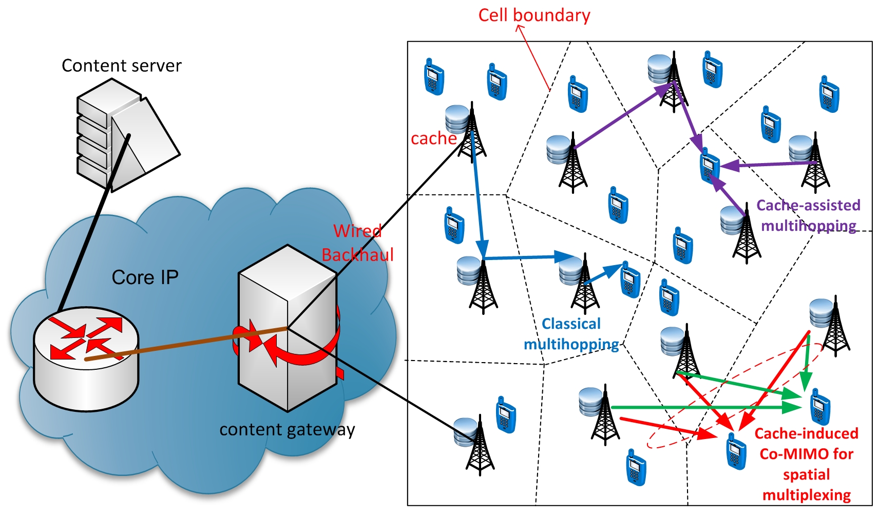
Figure 1: Architecture of the backhaul-limited C-DWN.

Consider a backhaul-limited C-DWN with $N$ BSs and $K$ users placed on a square of area $Nr_{0}^{2}$ as illustrated in Fig. 1. Each BS has an average transmit power budget of $P$ and a cache of limited size $B_{C}$ bits. Only $N_{0}\ll N$ BSs have wired backhaul connections with the core network. We divide the square into $N$ cells. The $n$-th cell is the set of all points which are closer to the $n$-th BS. If a user $k$ lies in the $n$-th cell, user $k$ is said to be associated with BS $n$. Let $b_{k}$ denote the BS associated with user $k$. We have the following assumption on the BS and user placement.

Assumption 1 (BS and User Placement).

The BS and user placement satisfies the following conditions.

1. The distance between any two BSs is no less than $r_{\textrm{min}}$

2. The distance between a BS and a user is no less than $d_{\textrm{min}}$.

3. For any point in the $n$-th cell, the distance between this point and the $n$-th BS is no more than $r_{\textrm{max}}$.

4. Each BS is associated with at most $k_{\textrm{max}}$ users, where $k_{\textrm{max}}$ is constant.

5. The total numbers of users and BSs satisfy $K=\Theta\left(N\right)$.

Assumption 1-1) means that the BS density at any local area does not go to infinity, which is always satisfied in practice. Assumption 1-2) means that the distance between any user and its associated BS is bounded away from zero so that the receive SNR at any user is bounded. Assumption 1-3) means that the size of any cell is bounded so that the received SNR of any user at any location is sufficiently large to establish a communication link between this user and the network. This assumption is used to ensure that there is no coverage hole in the network. Assumption 1-4) means that the user density at each cell does not go to infinity. Finally, Assumption 1-5) means that we consider a heavily loaded system where there are active users in most of the cells (BSs).

A large portion of the traffic in future wireless networks will come from content delivery applications where users obtain content (e.g., video) from the content server via the BSs and core network as illustrated in Fig. 1. There are $L$ content files on the content server and the size of each file is $F$ bits. For convenience, let $l_{k}$ denote the index of the file requested by the $k$-th user and let $\vec{l}=\left\{l_{1},...,l_{K}\right\}$ denote the user request profile (URP). Assume that each node independently accesses the $l$-th content file with probability $p_{l}$, where probability mass function $\mathbf{p}=\left[p_{1},...,p_{L}\right]$ represents the popularity of the content files. Without loss of generality, suppose $p_{1}\geq p_{2}\geq...\geq p_{L}$. In the rest of the paper, we focus on the non-trivial case when each BS does not have enough cache to store all the $L$ files, i.e., $B_{C}<LF$.

II-B Cached and Uncached Dense Wireless Networks

Suppose user $k$ is associated with a BS which has no wired backhaul. Without PHY caching, user $k$ has to obtain the requested content from the content server via the core network, wired backhaul, and multihop wireless links, as illustrated in Fig. 1 for the blue data flow. As a result, the user throughput is fundamentally limited by the multihop wireless inter-BS communications. For convenience, the backhaul-limited dense wireless networks without PHY caching is called the backhaul-limited uncached dense wireless networks (U-DWN).

In this paper, we propose a new architecture called the cached dense wireless network (C-DWN), where the BSs can cache some of the content from the content servers. If the content requested by a user is in the caches of the nearby BSs, this user can directly obtain the requested content from the nearby BSs via cache-induced opportunistic Co-MIMO (as illustrated in Fig. 1 for the red and green data flows) or cache-assisted multihopping (as illustrated in Fig. 1 for the purple data flow), depending on the cache state of the nearby BSs. An interesting question is that, what are the optimal capacity scaling and the corresponding optimal achievable scheme in C-DWN. This question will be answered in this paper.

II-C Channel Model

We use similar channel model as in [13], where the wireless link between any two nodes is a flat fading channel with bandwidth $W$. The channel coefficient between BS $n$ and BS $n^{{}^{\prime}}$ at time $t$ is

$$h_{n^{{}^{\prime}},n}^{b}\left(t\right)=\sqrt{G^{b}}\left(r_{n^{{}^{\prime}},n}^{b}\right)^{-\alpha/2}\exp\left(j\theta_{n^{{}^{\prime}},n}^{b}\left(t\right)\right),$$

where $r_{n^{{}^{\prime}},n}^{b}$ is the distance between BS $n$ and BS $n^{{}^{\prime}}$, $\theta_{n^{{}^{\prime}},n}^{b}\left(t\right)$ is the random phase at time $t$, $G^{b}$ is some constant depending on the transmitter and receiver antenna gains at the BSs, and $\alpha>2$ is the path loss exponent. Similarly, the channel between BS $n$ and user $k$ at time $t$ is given by

$$h_{k,n}^{d}\left(t\right)=\sqrt{G^{d}}\left(r_{k,n}^{d}\right)^{-\alpha/2}\exp\left(j\theta_{k,n}^{d}\left(t\right)\right),$$

where $r_{k,n}^{d}$ is the distance between BS $n$ and user $k$, $\theta_{k,n}^{d}\left(t\right)$ is the random phase, and $G^{d}$ is some constant. We assume that $\theta_{n^{{}^{\prime}},n}^{b}\left(t\right)$ and $\theta_{k,n}^{d}\left(t\right)$ are i.i.d. (w.r.t. the node index $n^{{}^{\prime}},n,k$ and time index $t$) with uniform distribution on $\left[0,2\pi\right]$. At each node, the received signal is corrupted by a circularly symmetric Gaussian noise with spectral density $\eta_{0}$.

II-D Offline Cache Initialization

There are two phases during the operation of cached wireless networks: the cache initialization phase and content delivery phase. In the cache initialization phase, each BS caches a portion of $q_{l}F$ (possibly encoded) bits of the $l$-th content file ($\forall l$), where $\mathbf{q}=\left[q_{1},...,q_{L}\right]^{T}$ (with $q_{l}\in\left[0,1\right]$ and $\sum_{l=1}^{L}q_{l}F\leq B_{C}$) are called cache content replication vector. The cache content replication vector $\mathbf{q}$ and the corresponding content stored at each BS is slowly adaptive to the popularity of files according to some caching scheme. The cache initialization phase restarts whenever the popularity changes. After each BS received the content determined by the caching scheme, the content delivery phase starts. Let $t_{C}$ denote the interval between two consecutive cache initialization phase. Since the popularity of content files change very slowly (e.g., new movies are usually posted on a weekly or monthly timescale), $t_{C}$ is large and thus the cache update overhead in the cache initialization phase is usually small compared to the PHY caching gain. In this paper, we assume that $t_{C}$ is sufficiently large and thus the cache update overhead can be ignored. We will focus on studying the content delivery phase.

III Capacity Bound of Backhaul-Limited U-DWN

In this section, we give an information theoretic upper bound on the aggregate throughput of the backhaul-limited U-DWN, which serves as benchmarking to quantify the gain due to PHY caching later.

For convenience, let $\mathcal{B}_{P}$ denote the set of $N_{0}$ backhaul-connected BSs. Let $\mathbf{H}_{b}=\left[h_{n^{{}^{\prime}},n}^{b}\right]_{\forall n^{{}^{\prime}}\in\left\{1,...,N\right\}\backslash\mathcal{B}_{P},n\in\mathcal{B}_{P}}\in\mathbb{C}^{\left(N-N_{0}\right)\times N_{0}}$ denote the composite channel between the $N_{0}$ backhaul-connected BSs and all other BSs. Let $\mathbf{H}_{d}=\left[h_{k,n}^{d}\right]_{\forall k,n\in\mathcal{B}_{P}}\in\mathbb{C}^{K\times N_{0}}$ denote the composite channel between the $N_{0}$ backhaul-connected BSs and all users. The following lemma is useful for deriving the capacity upper bound of the backhaul-limited U-DWN.

Lemma 1.

Let $\tilde{\mathbf{H}}=\left[\mathbf{H}_{b}^{T},\mathbf{H}_{d}^{T}\right]^{T}\in\mathbb{C}^{\left(N-N_{0}+K\right)\times N_{0}}$ denote the composite channel between the $N_{0}$ backhaul-connected BSs and all other nodes. The aggregate throughput of the backhaul-limited U-DWN is bounded above by

$$\tilde{T}\leq W\max_{\tilde{\mathbf{Q}}\left(\tilde{\mathbf{H}}\right)\succeq\mathbf{0},\textrm{E}\left[\textrm{Tr}\left(\tilde{\mathbf{Q}}\left(\tilde{\mathbf{H}}\right)\right)\right]\leq N_{0}P}\textrm{E}\left[\log\left|\mathbf{I}+\tilde{\mathbf{H}}\tilde{\mathbf{Q}}\left(\tilde{\mathbf{H}}\right)\tilde{\mathbf{H}}^{\dagger}\right|\right].$$ (1)

Moreover, we have $\textrm{Tr}\left(\tilde{\mathbf{H}}\tilde{\mathbf{H}}^{\dagger}\right)=\tilde{b}_{U}=\Theta\left(N_{0}\right),\forall\tilde{\mathbf{H}}$, where

$$\tilde{b}_{U}=\sum_{n\in\mathcal{B}_{P}}\sum_{n^{{}^{\prime}}\notin\mathcal{B}_{P}}G^{b}\left(r_{n^{{}^{\prime}},n}^{b}\right)^{-\alpha}+\sum_{n\in\mathcal{B}_{P}}\sum_{k=1}^{K}G^{d}\left(r_{k,n}^{d}\right)^{-\alpha}$$

Using Lemma 1, we can prove the following theorem.

Theorem 1 (Capacity upper bound of backhaul-limited U-DWN).

Define a function

$$f\left(\xi,x\right)=\begin{cases}\log\left(1+\xi x^{2}\right),&x\geq\sqrt{\frac{\zeta}{\xi}}\\ \frac{2\sqrt{\xi\zeta}}{1+\zeta}x,&x\in\left[0,\sqrt{\frac{\zeta}{\xi}}\right)\end{cases},$$

where $\xi=\frac{\tilde{b}_{U}}{N_{0}P}$, $\zeta=-1+e^{2+W_{0}\left(-2e^{-2}\right)}\approx 3.9216$, and $W_{0}\left(z\right)$ is the principal branch of the Lambert W function. Then the aggregate throughput of the backhaul-limited U-DWN is bounded above by

$$\tilde{T}\leq N_{0}Wf\left(\xi,P\right)=\Theta\left(N_{0}\right).$$

Please refer to Appendix -A for the proof of Lemma 1 and Theorem 1.

IV Capacity Scaling in Backhaul-Limited C-DWN

We first give an information theoretic upper bound on the aggregate throughput. The following lemma is useful for deriving the capacity upper bound.

Lemma 2.

Let $\mathbf{H}=\left[h_{k,n}^{d}\right]_{\forall k,n}\in\mathbb{C}^{K\times N}$ denote the composite channel between all BSs and all users. The aggregate throughput of the backhaul-limited C-DWN is bounded by

$$T\leq W\max_{\mathbf{Q}\left(\mathbf{H}\right)\succeq\mathbf{0},\textrm{E}\left[\textrm{Tr}\left(\mathbf{Q}\left(\mathbf{H}\right)\right)\right]\leq NP}\textrm{E}\left[\log\left|\mathbf{I}+\mathbf{H}\mathbf{Q}\left(\mathbf{H}\right)\mathbf{H}^{\dagger}\right|\right].$$ (2)

Moreover, we have $\textrm{Tr}\left(\mathbf{H}\mathbf{H}^{\dagger}\right)=b_{U}=\Theta\left(N\right),\forall\mathbf{H}$, where

$$b_{U}=\sum_{n=1}^{N}\sum_{k=1}^{K}G^{d}\left(r_{k,n}^{d}\right)^{-\alpha}.$$

Using Lemma 2, we can prove the following result.

Theorem 2 (Capacity upper bound of backhaul-limited C-DWN).

The aggregate throughput of the backhaul-limited C-DWN is bounded above by

$$T\leq NWf\left(\frac{b_{U}}{NP},P\right)=\Theta\left(N\right).$$

The proof of Lemma 2 and Theorem 2 is similar to that of Lemma 1 and Theorem 1 in Appendix -A. Next, we give the achievable throughput scaling laws. Define $\tilde{L}=\frac{LF}{B_{C}}$ as the normalized content size. Let the notation $N,\tilde{L}\overset{\iota}{\rightarrow}\infty$ denote $N\rightarrow\infty$ and $\lim_{N\rightarrow\infty}\frac{\tilde{L}}{N}=\iota\in\left[0,\infty\right)$. There are two classes of scaling laws depending on the normalized content size $\tilde{L}$.

Theorem 3 (Achievable throughput scaling laws with $\tilde{L}=\Theta\left(1\right)$).

In the backhaul-limited C-DWN, a per user throughput of $R=\Theta\left(1\right)$ is achievable when $N\rightarrow\infty$ and $\tilde{L}=\Theta\left(1\right)$. As a result, an aggregate throughput of $KR=\Theta\left(N\right)$ is also achievable.

When $\tilde{L}$ goes to infinity, the throughput scaling laws will also depend on the content popularity distribution. We make the following assumptions on the content popularity.

Assumption 2 (Content popularity).

The content popularity is modeled by the Zip distribution [29]:

$$p_{l}=\frac{1}{Z_{\tau}\left(L\right)}l^{-\tau},l=1,...,L,$$ (3)

where $\tau$ is the popularity skewness parameter, and $Z_{\tau}\left(L\right)=\sum_{l=1}^{L}l^{-\tau}$ is a normalization factor.

Theorem 4 (Achievable throughput scaling laws with Large $\tilde{L}$).

In the backhaul-limited C-DWN, a per user throughput of $R$ is achievable when $N,\tilde{L}\overset{\iota}{\rightarrow}\infty$, where

$$R=\begin{cases}\Theta\left(1/\sqrt{\tilde{L}}\right),&if\>0\leq\tau<1\\ \min\left(\Theta\left(\log L/\sqrt{\tilde{L}}\right),\Theta\left(1\right)\right)&if\>\tau=1\\ \min\left(\Theta\left(L^{\tau-1}/\sqrt{\tilde{L}}\right),\Theta\left(1\right)\right)&if\>1<\tau<\frac{3}{2}\\ \min\left(\Theta\left(\sqrt{L}\log^{-3/2}L/\sqrt{\tilde{L}}\right),\Theta\left(1\right)\right)&if\>\tau=3/2\\ \Theta\left(1\right),&if\>\tau>3/2\end{cases}$$

The proof of Theorem 3 and 4 relies on the construction of an achievable scheme that realizes the promised scaling law. The details will be given in Section V. Theorem 4 and Theorem 2 together establish the linear capacity scaling law in the backhaul-limited C-DWN when the normalized cache size $\tilde{B}_{C}=B_{C}/F$ is sufficiently large. Specifically, the following corollary from Theorem 3 and 4 quantifies the minimum normalized cache size $\tilde{B}_{C}^{\textrm{min}}$ needed to achieve the linear capacity scaling law.

Corollary 1 (Minimum cache size to achieve linear capacity scaling).

When $L=\Theta\left(1\right)$, the order of the minimum normalized cache size needed to achieve the linear capacity scaling $R=\Theta\left(1\right)$ is $\tilde{B}_{C}^{\textrm{min}}=\Theta\left(1\right)$. When $N,\tilde{L}\overset{\iota}{\rightarrow}\infty$, we have

$$\tilde{B}_{C}^{\textrm{min}}=\begin{cases}\Theta\left(L\right)&if\>0\leq\tau<1\\ \Theta\left(L/\log^{2}L\right)&if\>\tau=1\\ \Theta\left(L^{3-2\tau}\right)&if\>1<\tau<3/2\\ \Theta\left(\log^{3}L\right)&if\>\tau=3/2\\ \Theta\left(1\right)&if\>\tau>3/2\end{cases}$$

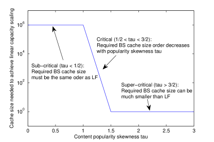
Figure 2: Phase transition of minimum BS cache size $B_{C}$ needed to achieve the linear capacity scaling for large $L$.

For a larger $\tau$, the requests will concentrate more on a few content files and thus a smaller BS cache is needed to achieve the linear capacity scaling law. When $N,\tilde{L}\overset{\iota}{\rightarrow}\infty$, there are two critical popularity skewness points: $\tau=1$ and $\tau=3/2$, as illustrated in Fig. 2. For the super-critical case when $\tau>3/2$, the linear capacity scaling laws can be achieved even when the cache size at each BS is much smaller than the total content size (i.e., $B_{C}=\Theta\left(1\right)$ and $LF\rightarrow\infty$). The intuition behind this result is as follows. When $\tau>3/2$, the user requests concentrate heavily on the $\Theta\left(1\right)$ most popular files such that we can ignore the impact of requesting the other $L-\Theta\left(1\right)$ files on the throughput scaling law. In this case, we can achieve the linear capacity scaling law by letting each BS cache a portion of $\frac{B_{C}}{F\Theta\left(1\right)}$ bits for each of the $\Theta\left(1\right)$ most popular files. This is because under such caching scheme, whenever a user requests one of the $\Theta\left(1\right)$ most popular files, the requested file must exist in the nearest $\Theta\left(1\right)$ BSs and thus the number of hops from the source BSs to the destination user is $\Theta\left(1\right)$. As a result, we can achieve the linear capacity scaling since the probability of requesting the other $L-\Theta\left(1\right)$ files is negligible when $\tau>3/2$. On the other hand, for the sub-critical case when $\tau<1$, the BS cache size $B_{C}$ must scale at the same order as the content size $LF$ in order to achieve the linear capacity scaling. The intuition behind this result is as follows. When $\tau<1$, the popularity is very flat such that the order of the minimum BS cache size $B_{C}$ needed to achieve the linear capacity scaling is the same as that of the extremely case when the popularity is completely flat (i.e., $p_{l}=\frac{1}{L},\forall l$). In this case, the optimal caching scheme is uniformly caching (i.e., $q_{l}=\frac{B_{C}}{FL},\forall l$) due to the symmetry of different files, and thus the requested file of any user must exist in the nearest $\Theta\left(\frac{FL}{B_{C}}\right)$ BSs. Clearly, if we want to achieve the linear capacity scaling, we must have $\frac{FL}{B_{C}}=\Theta\left(1\right)$, i.e., $B_{C}=\Theta\left(LF\right)$.

According to Theorem 3 and 4, we can achieve linear capacity scaling law in the backhaul-limited C-DWN with only a fixed number of wired payload backhauls $N_{0}$ by a proper PHY caching scheme, when the cache size $B_{C}$ is sufficiently large. Moreover, the required cache size to achieve the linear capacity scaling law decreases with the popularity skewness $\tau$. These results have fundamental impact on future wireless networks. Since the cost of storage device is much lower than the cost of wired backhaul, and the popularity skewness $\tau$ can be large for mobile applications [29], the backhaul-limited C-DWN provides a promising architecture for future wireless networks.

V Order-optimal Capacity Achieving Scheme

In this section, we propose an achievable PHY caching and transmission scheme (abbreviated as Scheme A) which can achieve the throughput scaling laws in Theorem 3 and 4. There are two major components: the two-mode maximum distance separable (MDS) coded caching working in the cache initiation phase and the cache-assisted PHY transmission working in the content delivery phase. The two-mode MDS-coded caching decides how to cache the coded segments at each BS and the cache-assisted PHY transmission contains two modes, namely, the cache-assisted multihop transmission mode and cache-induced Co-MIMO transmission mode. They are elaborated below.

V-A Two-mode MDS-coded Caching Scheme

The cache-assisted multihopping and cache-induced opportunistic Co-MIMO have conflicting requirements on the caching scheme. For the former, it is better to cache different content at different BSs. For the later, it is better to cache the same content at nearby BSs to create a MIMO cooperation opportunity. We propose a two-mode MDS-coded caching scheme to strike a balance between them. There are two cache modes depending on the popularity of the cached files. The Co-MIMO cache mode is used for popular files to induce MIMO cooperation opportunity, and the multihop cache mode is used for less popular files to achieve cache-assisted multihopping gain. The details are summarized below.

Step 1 (MDS Encoding and Cache Modes Determination): At the content server, each file is divided into segments of size $L_{S}$ bits and each segment is encoded using an ideal MDS rateless code. If $q_{l}=1$, the cache mode for the $l$-th file is set to be Co-MIMO cache mode. In this case, for each segment of the $l$-th file, the MDS encoder generates one Co-MIMO parity block of length $L_{S}$ bits. If $q_{l}<1$, the cache mode for the $l$-th file is set to be multihop cache mode and the MDS encoder generates $N$ multihop parity blocks of length $q_{l}L_{S}$ for each segment of the $l$-th file. Define $\Omega\left(\mathbf{q}\right)\triangleq\left\{l:\>q_{l}<1\right\}$ as the set of files associated with multihop cache mode and $\overline{\Omega}\left(\mathbf{q}\right)\triangleq\left\{l:\>q_{l}=1\right\}$ as the set of files associated with Co-MIMO cache mode.

Step 2 (Offline Cache Initialization): For $l=1,..,L$, if $l\in\Omega\left(\mathbf{q}\right)$, then the cache of BS $n$ is initialized with the $n$-th multihop parity block for each segment of the $l$-th file. If $l\in\overline{\Omega}\left(\mathbf{q}\right)$, then the caches of all the BSs are initialized with the Co-MIMO parity block for each segment of the $l$-th file.

We use an example to illustrate the above caching scheme with $2$ files. The first file is popular, and the Co-MIMO cache mode is used ($q_{1}=1$). The second file is less popular, and the multihop cache mode is used ($q_{2}=0.5$). The size of each file is $3$Mbits and the segment size is $L_{S}=1$Mbits. There are two BSs and the cache size $B_{C}$ is $4.5$Mbits. For file 1, the content server only generates a single Co-MIMO parity block of length 1Mbits from each segment (there are totally 3 Co-MIMO parity blocks). BS 1 and BS 2 cache the same Co-MIMO parity block of every segment of file 1. For file 2, the content server generates two multihop parity blocks of length 0.5Mbits from each segment (there are totally 6 multihop parity blocks). BS 1 (2) caches the first (second) multihop parity block of every segment of file 2.

The achievable throughput depends on the choice of the cache content replication vector $\mathbf{q}$. In Theorem 5, we will give an order-optimal cache content replication vector $\mathbf{q}$ to maximize the order of the per user throughput.

V-B PHY Mode Determination and Frequency Partitioning

The transmission mode for a requested file is determined by the cache mode. Specifically, a requested file $l\in\Omega\left(\mathbf{q}\right)$ ($l\in\overline{\Omega}\left(\mathbf{q}\right)$) associated with the multihop cache mode (Co-MIMO cache mode) is delivered to the destination user using the cache-assisted multihop transmission (cache-induced Co-MIMO). To transmit a file $l\in\Omega\left(\mathbf{q}\right)$ to a user, the associated BS needs to first collect the requested parity bits from a set of source BSs (determined by source BS set selection) via wireless inter-BS transmission and then send them to this user via downlink access transmission, as illustrated in Fig. 3. Correspondingly, the system bandwidth $W$ is divided into three bands: the inter-BS band with size $W_{b}$ for wireless inter-BS transmission, the downlink access band with size $W_{d}$ for downlink access transmission, and the Co-MIMO band with size $W_{c}$ for Co-MIMO transmission, where $W_{b}+W_{d}+W_{c}=W$. As a result, these three transmissions can occur simultaneously without causing interference to each other.

V-C Cache-assisted Multihop Transmission

V-C1 Source BS Set Selection

For a user $k$ requesting a file $l\in\Omega\left(\mathbf{q}\right)$, the associated BS needs to select a set of source BSs to download the requested file segment. Intuitively, the associated BS should select the source BS set so as to reduce the number of hops and to balance the BS loads. We propose the following scheme to achieve this.

Step 1 (Source BS Set Selection): The associated BS chooses the nearest BSs (including the associated BS) which have a total number of $L_{S}$ parity bits of the requested file segment as the source BSs. Specifically, let $r_{k}^{*}=\min\>r,\>\textrm{s.t. }\left|\left\{n:\>r_{b_{k},n}\leq r\right\}\right|\geq\left\lceil 1/q_{l}\right\rceil$. Then the set of source BSs for user $k$ is given by $\mathcal{B}_{k}=\left\{n:\>r_{b_{k},n}\leq r_{k}^{*}\right\}$.

Step 2 (Load Partitioning): The associated BS determines the load partition among the source BSs as follows. For convenience, define $\overline{\mathcal{B}}_{k}=\left\{n:\>r_{b_{k},n}<r_{k}^{*}\right\}$. Note that $\left|\overline{\mathcal{B}}_{k}\right|\leq\left\lceil 1/q_{l}\right\rceil-1$. For each requested file segment, user $k$ obtains $q_{l}L_{S}$ parity bits from each BS in $\overline{\mathcal{B}}_{k}$ and $\frac{\left(1-\left|\overline{\mathcal{B}}_{k}\right|q_{l}\right)L_{S}}{\left|\mathcal{B}_{k}\right|-\left|\overline{\mathcal{B}}_{k}\right|}$ parity bits from each BS in $\mathcal{B}_{k}\backslash\overline{\mathcal{B}}_{k}$.

The following lemma gives an upper bound for $r_{k}^{*}$.

Lemma 3.

For a user $k$ requesting a file $l\in\Omega\left(\mathbf{q}\right)$ associated with the multihop cache mode, we have

$$r_{k}^{*}\leq\left(2\sqrt{\left\lceil 1/q_{l}\right\rceil-1}+1\right)r_{\textrm{max}}.$$

Please refer to Appendix -B for the proof.

V-C2 Wireless Inter-BS Transmission

Frequency reuse is used to control the interference between the BSs on the inter-BS band. The inter-BS bandwidth $W_{b}$ is uniformly divided into $M_{b}$ subbands and each BS is allocated with one subband such that the following condition is satisfied.

Condition 1.

Any two BSs with distance no more than $r_{I}^{b}$ is allocated with different subbands, where $r_{I}^{b}>2r_{\textrm{max}}$ is a system parameter.

The following lemma gives the number of subbands that is required to satisfy the above condition.

Lemma 4.

There exists a frequency reuse scheme which has $M_{b}\leq\left(\frac{2r_{I}^{b}}{r_{\textrm{min}}}+1\right)^{2}+1$ subbands and satisfies Condition 1.

Please refer to Appendix -B for the proof.

We now elaborate the wireless inter-BS transmission scheme for a user $k$ requesting a file $l\in\Omega\left(\mathbf{q}\right)$. For any source BS $n^{{}^{\prime}}$other than the associated BS $n=b_{k}$, we draw a routing line segment $\mathcal{L}_{n^{{}^{\prime}},n}$ between BS $n^{{}^{\prime}}$ and BS $n$. This routing line segment intersects several cells. Then the parity bits requested by the user are relayed from BS $n^{{}^{\prime}}$ to the BS $n$ in a sequence of hops. In each hop, the parity bits are transferred from one cell (BS) to another in the order in which they intersect the routing line segment, as illustrated in Fig. 3.

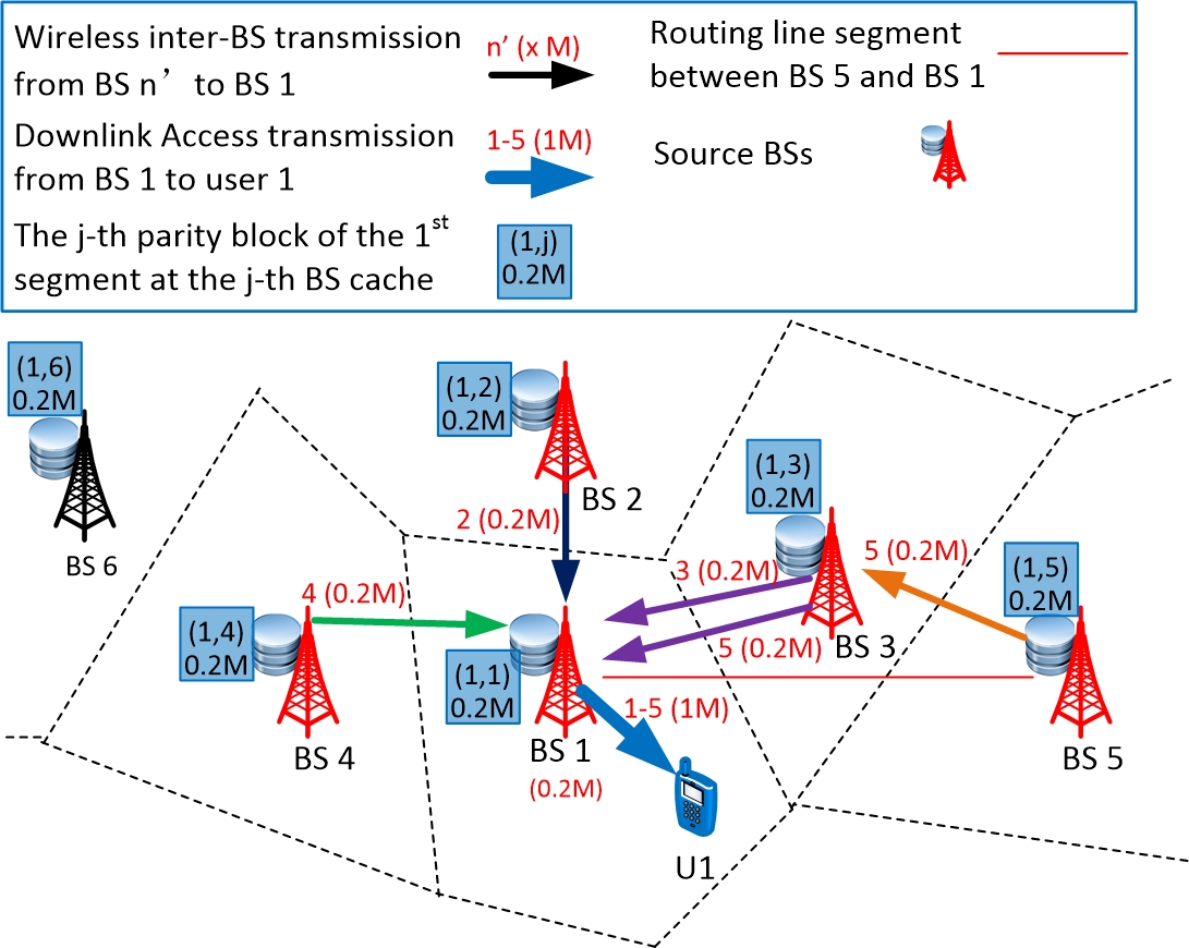
Figure 3: An illustration of cache-assisted multihop transmission, where user $1$ requests the first segment (with size $L_{S}=1$Mbits) of a file associated with multihop caching mode. The requested file segment is encoded into parity blocks of 0.2Mbits at the content server and each BS caches one parity block (0.2M parity bits).

For convenience, we call $\left\{\mathcal{L}_{n^{{}^{\prime}},b_{k}},\forall n^{{}^{\prime}}\in\mathcal{B}_{k}\backslash\left\{b_{k}\right\}\right\}$ the set of routing line segments of user $k$. The following lemma is useful when deriving the lower bound for the achievable rates.

Lemma 5.

For any $n$, the average number of users whose routing line segments intersect cell $n$ is upper bounded by

$$J\triangleq\sum_{l=1}^{L}p_{l}\left(\frac{\left(4\sqrt{\left\lceil 1/q_{l}\right\rceil-1}+2\right)r_{\textrm{max}}}{r_{\textrm{min}}}+1\right)^{2}k_{\textrm{max}}.$$

Please refer to Appendix -B for the proof.

V-C3 Downlink Access Transmission for Cache-assisted Multihop

For a user $k$ requesting a file $l\in\Omega\left(\mathbf{q}\right)$, the wireless inter-BS transmission scheme ensures that all the segments (parity bits) requested by user $k$ are available at the associated BS $b_{k}$. Then the associated BS $b_{k}$ sends the requested parity bits to user $k$ using downlink access transmission. To control the inter-cell interference, the downlink access bandwidth $W_{d}$ is uniformly divided into $M_{d}\leq\left(\frac{2r_{I}^{d}}{r_{\textrm{min}}}+1\right)^{2}+1$ subbands and each BS is allocated with one subband such that any two BSs with distance no more than $r_{I}^{d}$ is allocated with different subbands, where $r_{I}^{d}>r_{\textrm{max}}$ is a system parameter. Within each cell, a simple TDMA scheme is used to mitigate the multi-user interference in the downlink access transmission, where at each time slot, only one user is scheduled for transmission in a round robin fashion.

The overall cache-assisted multihop transmission is summarized in Fig. 3. The cache-assisted multihop transmission contains 3 steps.

Step 1 (source BS set selection): The associated BS (BS 1) chooses the nearest BSs (including BS 1) which have a total number of 1M parity bits of the requested file segment as the source BS set (which is $\left\{1,...,5\right\}$). The load partition among the source BSs is illustrated in red above each data flow (colored arrow). Step 2 (wireless inter-BS transmission): The wireless inter-BS transmission between a source BS, say BS 5, and the associated BS is as follows. We first draw a routing line segment between BS 5 and BS 1 (red line). The routing line segment intersects cell 3 and cell 1. Then BS 5 sends the parity bits requested by user $1$ to the associated BS (BS 1) via wireless inter-BS transmission over the route BS 5$\rightarrow$BS 3$\rightarrow$BS 1. Step 3 (downlink access transmission): BS 1 transmits the collected 1M parity bits (0.2Mbits from the local cache and 0.8Mbits from the other source BSs) of the requested file segment to user $1$ via downlink access transmission. Note that the arrows with different colors represent the transmissions on different subbands for interference control.

V-D Cache-induced Co-MIMO Transmission

For a user requesting a file $l\in\overline{\Omega}\left(\mathbf{q}\right)$, the requested segment exists at all BS caches. As a result, the BSs can employ Co-MIMO to improve the PHY performance. The cache-induced Co-MIMO scheme contains the following three steps.

Step 1 (BS clustering): At each time slot, the whole area is partitioned into squares of size $N_{c}r_{0}^{2}$, where $N_{c}$ determines the BS cluster size. Then the BSs in the same square forms a cluster.

Step 2 (User scheduling in each cluster): Without loss of generality, we consider the $j$-th cluster. Let $\mathcal{G}_{j}^{B}$ denote the set of BSs in the $j$-th cluster and let $\mathcal{G}_{j}^{K}\triangleq\left\{k:\>b_{k}\in\mathcal{G}_{j}^{B},l_{k}\in\overline{\Omega}\left(\mathbf{q}\right)\right\}$ denote the set of users which are associated with the BSs in $\mathcal{G}_{j}^{B}$. At each time slot, $K_{j}^{S}=\min\left(\left|\mathcal{G}_{j}^{K}\right|,\left|\mathcal{G}_{j}^{B}\right|\right)$ users in $\mathcal{G}_{j}^{K}$ are scheduled for transmission in a round robin fashion.

Step 3 (Co-MIMO transmission in each cluster): In the $j$-th cluster, the $\left|\mathcal{G}_{j}^{B}\right|$ BSs employ Co-MIMO to jointly transmit some parity bits to the scheduled $K_{j}^{S}$ users.

Finally, we adopt uniform power allocation where the power allocated to each subband is proportional to the bandwidth of the subband. For example, at each BS, the power allocated on each subband of the wireless inter-BS transmission is $\frac{W_{b}P}{M_{b}W^{{}^{\prime}}}$, the power allocated on each subband of the downlink access transmission is $\frac{W_{d}P}{M_{d}W^{{}^{\prime}}}$, and the power allocated on the Co-MIMO band is $\frac{W_{c}P}{W^{{}^{\prime}}}$, where $W^{{}^{\prime}}=\frac{W_{b}}{M_{b}}+\frac{W_{d}}{M_{d}}+W_{c}$. The total transmit power of a BS is given by $P$.

V-E Order Optimality Analysis

The order optimality of Scheme A is summarized in the following theorem.

Theorem 5 (Order optimality of Scheme A).

In the backhaul-limited C-DWN, a per user throughput of

$$R=\Theta\left(\frac{W}{\sum_{l=1}^{L}p_{l}\sqrt{\frac{1}{q_{l}}}}\right)$$ (4)

can be achieved by Scheme A. Moreover, the order-optimal cache content replication vectors $\mathbf{q}^{*}$ and the corresponding per user throughput orders for different cases are given below.

1. When the normalized content size $\tilde{L}=\Theta\left(1\right)$ and $N\rightarrow\infty$, an order-optimal cache content replication vector is given by $q_{l}^{*}=\frac{B_{C}}{LF},l=1,...,L$, and the corresponding per user throughput order is $\Theta\left(1\right)$.

2. When $N,\tilde{L}\overset{\iota}{\rightarrow}\infty$, an order-optimal cache content replication vector is given by

   $$q_{l}^{*}=\min\left(\frac{B_{C}}{F}\frac{p_{l}^{2/3}}{\sum_{l=1}^{L}p_{l}^{2/3}},1\right),l=1,...,L,$$ (5)

   and the corresponding per user throughput order is the same as that in Theorem 4.

The factor $\sum_{l=1}^{L}p_{l}\sqrt{\frac{1}{q_{l}}}$ in (4) is due to the wireless inter-BS transmission and it determines the order of per user throughput. According to Lemma 5, the traffic to be relayed by a BS due to wireless inter-BS transmission is upper bounded by $JR$, where $J=\Theta\left(\sum_{l=1}^{L}p_{l}\sqrt{\frac{1}{q_{l}}}\right)$. Since the capacity of a BS on the inter-BS band is $\Theta\left(1\right)$, we must have $R\leq\Theta\left(1/J\right)$. Hence, the capacity order of the backhaul-limited C-DWN is mainly limited by the wireless inter-BS transmission. Please refer to Appendix -C for the detailed proof of Theorem 5.

VI What is the Role of Cache-induced Co-MIMO?

Since the cache-induced Co-MIMO cannot improve scaling laws, an important question is that, what is the role of cache-induced Co-MIMO and is it worthwhile to exploit cache-induced Co-MIMO? In this section, we are going to answer this question by comparing Scheme A with a baseline scheme called Scheme B, which exploits purely the cached-assisted multihopping benefit in C-DWN. In Scheme B, there is no cache-induced Co-MIMO transmission as depicted in Section V-D. As a result, we have $W_{c}=0$ and $W_{b}+W_{d}=W$. The PHY transmission scheme for requesting a file $l\in\Omega\left(\mathbf{q}\right)$ is based on the cache-assisted multihop transmission summarized in Fig. 3. On the other hand, a requested file $l\in\overline{\Omega}\left(\mathbf{q}\right)$ is delivered from the associated BS to the destination user using the downlink access transmission described in V-C3 since all the segments of a file $l\in\overline{\Omega}\left(\mathbf{q}\right)$ exist in the caches of all BSs.

We will first analyze the per BS throughput of Scheme A and B in the regular C-DWN defined below.

Definition 1 (Regular C-DWN).

In a regular C-DWN, the BSs are placed on a grid as illustrated in Fig. 4. The distance between the adjacent BSs is $r_{0}$. Each BS has four users and they are placed on the grid line around the BS. The distance between a user and the associated BS is $d_{0}<r_{0}/2$.

Then we will quantify the cache-induced MIMO cooperation gain, which is defined as the per BS throughput gap between Scheme A and Scheme B. In the following analysis, we let $N\rightarrow\infty$ to get rid of the boundary effect. We also assume symmetric traffic model where all users have the same throughput requirement $R$.

VI-A Closed-form Bounds for Per BS Throughput

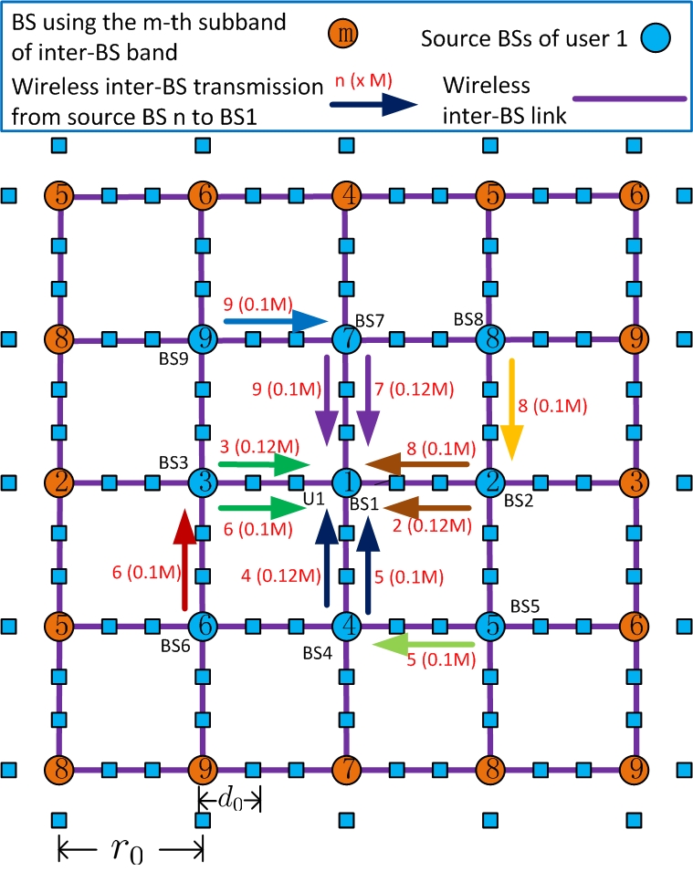
Figure 4: An illustration of cache-assisted multihop transmission in the regular C-DWN. User $1$ requests the $i$-th segment (with size $L_{S}=1$Mbits) of file $l$ associated with multihop caching mode. The requested file segment is encoded into parity blocks of 0.12Mbits at the content server and each BS caches one parity block (0.12M parity bits). The set of source BSs for user $1$ is $\left\{1,...,9\right\}$. The wireless inter-BS transmissions between the source BSs and the associated BS (BS1) are illustrated with colored arrows, where different colors represents different subbands. After collecting $1$M parity bits of the $i$-th segment from the source BSs, BS 1 transmits them to user 1 via downlink access transmission.

It is highly non-trivial to derive the exact expression for the per BS throughput especially for Scheme A with complicated cache-induced Co-MIMO transmission. In this section, we derive closed-form bounds for per BS throughput which are asymptotically tight at high SNR. The common parameters in Scheme A and B are set as: $r_{I}^{b}=2.5r_{0}$ and $r_{I}^{d}=1.5r_{0}$. As a result, the inter-BS bandwidth $W_{b}$ is divided into $M_{b}=9$ subbands and the distance between a BS and its nearest interfering BS is $3r_{0}$ on the inter-BS band, as illustrated in Fig. 4. On the other hand, $M_{d}=4$ and it can be verified that the distance between a BS and its nearest interfering BS is $2r_{0}$ on the downlink access band. In Fig. 4, we illustrate the cache-assisted multihop transmission for a regular C-DWN. According to the wireless inter-BS transmission scheme in Section V-C2, only the adjacent BSs can communicate with each other and the wireless link between two adjacent BSs is called a wireless inter-BS link as illustrated in Fig. 4.

First, we derive the average rate of each wireless inter-BS link and the per user downlink access transmission rate in the cache-assisted multihop transmission.

Lemma 6.

The average rate of each wireless inter-BS link is $W_{b}R_{b}\left(W_{b},W_{c}\right)$, where

$$R_{b}\left(W_{b},W_{c}\right)=\frac{1}{36}\log\left(1+\frac{PG^{b}r_{0}^{-\alpha}}{W^{{}^{\prime}}\eta_{0}+PG^{b}I_{R}\left(1,3\right)}\right),$$

$W^{{}^{\prime}}=\left(9W-5W_{b}+27W_{c}\right)/36$, and

$$I_{R}\left(x,y\right)$$

$$= \sum_{i=1}^{\infty}\frac{1}{r_{0}^{\alpha}}\left[\sum_{j=1}^{\infty}2\left(\left(yi+x\right)^{2}+y^{2}j^{2}\right)^{-\frac{\alpha}{2}}+\left|yi+x\right|^{-\alpha}\right]$$

$$+ \sum_{i=1}^{\infty}\frac{1}{r_{0}^{\alpha}}\left[\sum_{j=1}^{\infty}2\left(\left(yi-x\right)^{2}+y^{2}j^{2}\right)^{-\frac{\alpha}{2}}+\left|yi-x\right|^{-\alpha}\right]$$

$$+ \sum_{i=1}^{\infty}\frac{2}{r_{0}^{\alpha}}\left(y^{2}i^{2}+x^{2}\right)^{-\frac{\alpha}{2}}.$$

The per user average downlink access transmission rate is given by $W_{d}R_{d}\left(W_{b},W_{c}\right)$, where

$$R_{d}\left(W_{b},W_{c}\right)=\frac{1}{16}\log\left(1+\frac{PG^{d}d_{0}^{-\alpha}}{W^{{}^{\prime}}\eta_{0}+PG^{d}I_{R}\left(\frac{d_{0}}{r_{0}},2\right)}\right).$$

Please refer to Appendix -D for the proof of Lemma 6.

Clearly, $R_{b}$ is bounded as $R_{b}^{U}\geq R_{b}\left(W_{b},W_{c}\right)\geq R_{b}^{L}$, where

$$R_{b}^{U}=\frac{1}{36}\log\left(1+\frac{9PG^{b}r_{0}^{-\alpha}}{W\eta_{0}+9PG^{b}I_{R}\left(1,3\right)}\right),$$

$$R_{b}^{L} = \frac{1}{36}\log\left(1+\frac{PG^{b}r_{0}^{-\alpha}}{W\eta_{0}+PG^{b}I_{R}\left(1,3\right)}\right),$$

and $R_{d}$ is bounded as $R_{d}^{U}\geq R_{d}\left(W_{b},W_{c}\right)\geq R_{d}^{L}$, where

$$R_{d}^{U}=\frac{1}{16}\log\left(1+\frac{9PG^{d}d_{0}^{-\alpha}}{W\eta_{0}+9PG^{d}I_{R}\left(\frac{d_{0}}{r_{0}},2\right)}\right),$$

$$R_{d}^{L} = \frac{1}{16}\log\left(1+\frac{PG^{d}d_{0}^{-\alpha}}{W\eta_{0}+PG^{d}I_{R}\left(\frac{d_{0}}{r_{0}},2\right)}\right).$$

On the other hand, the average rate of a user on the Co-MIMO band has no closed-form expression. The following lemma gives closed-form bounds for the average Co-MIMO transmission rate.

Lemma 7 (Average rate bounds for cache-induced Co-MIMO).

Let $G_{C}=I_{R}\left(\frac{d_{0}}{r_{0}},1\right)+d_{0}^{-\alpha}$, $\rho=\frac{1}{2}\left(1-\frac{d_{0}^{-\alpha}}{G_{C}}\right)^{2}$, $R_{c}^{U}=\frac{1}{4}\log\left(1+\frac{9PG^{d}G_{C}}{W\eta_{0}}\right)$ and $R_{c}^{L}=\frac{\rho}{4}\log\left(1+\frac{PG^{d}d_{0}^{-\alpha}}{W\eta_{0}}\right)$. The average rate of a user on the Co-MIMO band is $W_{c}R_{c}\left(W_{b},W_{c}\right)$ , where $R_{c}\left(W_{b},W_{c}\right)$ is bounded as

$$R_{c}^{U}\geq R_{c}\left(W_{b},W_{c}\right)\geq R_{c}^{L}+O\left(PN_{c}^{-\frac{\alpha-2}{2\left(\alpha-1\right)}}\right).$$

Please refer to Appendix -E for the proof. Finally, using Lemma 6 and 7, the per BS throughput of Scheme A is bounded in the following theorem.

Theorem 6 (Per BS throughput bounds of Scheme A).

The per BS throughput $\Gamma_{A}\left(\mathbf{q}\right)$ of Scheme A is bounded as $\Gamma_{A}^{U}\left(\mathbf{q}\right)\geq\Gamma_{A}\left(\mathbf{q}\right)\geq\Gamma_{A}^{L}\left(\mathbf{q}\right)+O\left(PN_{c}^{-\frac{\alpha-2}{2\left(\alpha-1\right)}}\right)$ with

$$\Gamma_{A}^{a}\left(\mathbf{q}\right)=\frac{4R_{b}^{a}R_{c}^{a}R_{d}^{a}W}{Q_{\mathbf{q}}^{b}R_{c}^{a}R_{d}^{a}+Q_{\mathbf{q}}^{c}R_{b}^{a}R_{d}^{a}+Q_{\mathbf{q}}^{d}R_{b}^{a}R_{c}^{a}},$$ (6)

for $a\in\left\{L,U\right\}$, where $Q_{\mathbf{q}}^{b}=\sum_{l\in\Omega\left(\mathbf{q}\right)}p_{l}\psi\left(q_{l}\right)$, $Q_{\mathbf{q}}^{c}=\sum_{l\in\overline{\Omega}\left(\mathbf{q}\right)}p_{l}$, $Q_{\mathbf{q}}^{d}=\sum_{l\in\Omega\left(\mathbf{q}\right)}p_{l}$, and

$$\psi\left(q_{l}\right) = \phi\left(q_{l}\right)\left(1-q_{l}\right)-\frac{2}{3}\left(\phi^{3}\left(q_{l}\right)-\phi\left(q_{l}\right)\right)q_{l},$$ (7)

$$\phi\left(q_{l}\right) = \left\lceil\frac{-1+\sqrt{\frac{2}{q_{l}}-1}}{2}\right\rceil.$$

Finally, as $P,N_{c}\rightarrow\infty$ such that $PN_{c}^{-\frac{\alpha-2}{2\left(\alpha-1\right)}}\rightarrow 0$, we have

$$\Gamma_{A}\left(\mathbf{q}\right)\rightarrow\frac{W\tilde{R}_{b}\tilde{R}_{d}}{4Q_{\mathbf{q}}^{d}\tilde{R}_{b}+9Q_{\mathbf{q}}^{b}\tilde{R}_{d}},$$ (8)

where $\tilde{R}_{b}=\log\left(1+\frac{r_{0}^{-\alpha}}{I_{R}\left(1,3\right)}\right)$ and $\tilde{R}_{d}=\log\left(1+\frac{d_{0}^{-\alpha}}{I_{R}\left(\frac{d_{0}}{r_{0}},2\right)}\right)$.

Please refer to Appendix -F for the proof. The physical meaning of the terms $\phi\left(q_{l}\right)$ and $\psi\left(q_{l}\right)$ in Theorem 6 can be interpreted as follows. As can be seen in Fig. 4, for each BS, the number of BSs with the nearest distance ($r_{0}$) from the associated BS is $4$, that with the second nearest distance ($\sqrt{2}r_{0}$) is $8$, and that with the $m$-th nearest distance is $4m$. Let $\mathcal{B}_{k,m}$ denote the set of BSs with the $m$-th nearest distance from the associated BS. Suppose user $k$ requests file $l$. Then $\phi\left(q_{l}\right)$ is the maximum number of hops between the associate BS and the source BSs in $\mathcal{B}_{k}$ (e.g., in Fig. 4, the maximum number of hops between the associate BS of user $1$ and its source BSs is $\phi\left(0.12\right)=2$). Moreover, it can be shown that $\sum_{l\in\Omega\left(\mathbf{q}\right)}p_{l}\psi\left(q_{l}\right)R$ is the average traffic rate on the inter-BS band induced by a single user.

Following similar analysis, it can be shown that the per BS throughput $\Gamma_{B}\left(\mathbf{q}\right)$ of Scheme B at high SNR is given by

$$\Gamma_{B}\left(\mathbf{q}\right)\rightarrow\frac{W\tilde{R}_{b}\tilde{R}_{d}}{4\tilde{R}_{b}+9Q_{\mathbf{q}}^{B}\tilde{R}_{d}},\>\textrm{as}\>P\rightarrow 0.$$ (9)

VI-B Analysis of Cache-induced MIMO Cooperation Gain

From Theorem 6, we can obtain the following corollary which quantifies the cache-induced MIMO cooperation gain $\triangle\Gamma\triangleq\Gamma_{A}\left(\mathbf{q}^{*}\right)-\Gamma_{B}\left(\mathbf{q}^{*}\right)$ under the order-optimal cache content replication vector $\mathbf{q}^{*}$ in (5).

Corollary 2 (Cache-induced MIMO cooperation gain).

The cache-induced MIMO cooperation gain $\triangle\Gamma$ is bounded as $\triangle\Gamma_{U}\geq\triangle\Gamma\geq\triangle\Gamma_{L}+O\left(PN_{c}^{-\frac{\alpha-2}{2\left(\alpha-1\right)}}\right)$ with

$$\triangle\Gamma_{a} = \Gamma_{A}^{a}\left(\mathbf{q}^{*}\right)-\Gamma_{B}\left(\mathbf{q}^{*}\right),\>a\in\left\{L,U\right\},$$ (10)

where $\mathbf{q}^{*}$ is given in (5). Moreover, as $P,N_{c}\rightarrow\infty$ such that $PN_{c}^{-\frac{\alpha-2}{2\left(\alpha-1\right)}}\rightarrow 0$, we have $\triangle\Gamma\rightarrow\overline{\triangle\Gamma}$, where

$$\overline{\triangle\Gamma} = \frac{4W\tilde{R}_{b}\tilde{R}_{d}\left(1-Q_{\mathbf{q}^{*}}^{d}\right)\tilde{R}_{b}}{\left(4Q_{\mathbf{q}^{*}}^{d}\tilde{R}_{b}+9Q_{\mathbf{q}^{*}}^{b}\tilde{R}_{d}\right)\left(4\tilde{R}_{b}+9Q_{\mathbf{q}^{*}}^{B}\tilde{R}_{d}\right)}$$

$$= \Theta\left(\frac{\frac{B_{C}}{F}Q_{\mathbf{q}^{*}}^{c}}{\left[\sum_{l=1}^{L}p_{l}^{2/3}\right]^{3}}\right).$$

According to Corollary 2, the PHY caching gain can be well approximated by $\overline{\triangle\Gamma}$ at high SNR. $\overline{\triangle\Gamma}$ captures the key features of the actual (simulated) cache-induced MIMO cooperation gain as illustrated in Fig. 5. From (2), we have the following observations.

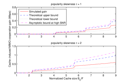
Figure 5: Impact of system parameters on the cache-induced MIMO cooperation gain in a regular C-DWN with $N=144$ BSs, $K=576$ users and $L=10$ files. The system bandwidth is 1MHz and SNR$=20$dB. The content popularity skewness $\tau=$1 in the upper subplot and $\tau=$2 in the lower subplot. The Co-MIMO cluster size is $N_{c}=9$.

Impact of the normalized cache size $\tilde{B}_{C}$: When $\tilde{B}_{C}<\sum_{l=1}^{L}l^{-\frac{2}{3}\tau}$, we have $q_{l}^{*}<1,\forall l$ and $\overline{\triangle\Gamma}=0$. When $\tilde{B}_{C}\geq\sum_{l=1}^{L}l^{-\frac{2}{3}\tau}$, $\overline{\triangle\Gamma}>0$ and $\overline{\triangle\Gamma}$ is an increasing function of $\tilde{B}_{C}$, as shown in Fig. 5. Note that as $\tilde{B}_{C}$ increases, $\overline{\triangle\Gamma}$ has positive jumps because $Q_{\mathbf{q}}^{d}$ is not a continuous function of $\tilde{B}_{C}$.

Impact of the Content Popularity Skewness $\tau$: As $\tau$ increases, the minimum normalized cache size $\tilde{B}_{C}$ needed to achieve a non-zero cache-induced MIMO cooperation gain decreases, and the gain $\overline{\triangle\Gamma}$ also increases for the same $\tilde{B}_{C}$, as illustrated in Fig. 5. When $\tau>\frac{3}{2}$, $\sum_{l=1}^{L}p_{l}^{2/3}=\Theta\left(\sum_{l=1}^{L}l^{-\frac{2}{3}\tau}\right)$ is bounded and we can achieve a cache-induced MIMO cooperation gain of $\Theta\left(1\right)$ even when the normalized cache size $\tilde{B}_{C}=\Theta\left(1\right)$ is fixed and $L\rightarrow\infty$. On the other hand, when $\tau\leq\frac{3}{2}$, the normalized cache size $\tilde{B}_{C}$ has to increase with $L$ at different orders as $L\rightarrow\infty$ in order to achieve a significant cache-induced MIMO cooperation gain as shown in the following corollary.

Corollary 3.

The order of the minimum normalized cache size $\tilde{B}_{C}^{\textrm{min}}$ needed to achieve a cache-induced MIMO cooperation gain of $\Theta\left(1\right)$ is the same as that needed to achieve the linear capacity scaling, as given in Corollary 1.

Hence, the minimum required cache size $\tilde{B}_{C}^{\textrm{min}}$ to achieve a large cache-induced MIMO cooperation gain decreases with the popularity skewness $\tau$, as shown in Fig. 2. When either the BS cache size $B_{C}$ is large, or the popularity skewness $\tau$ is large, the cache-induced MIMO cooperation gain is significant and it is worthwhile to exploit cache-induced Co-MIMO.

VII Numerical Results

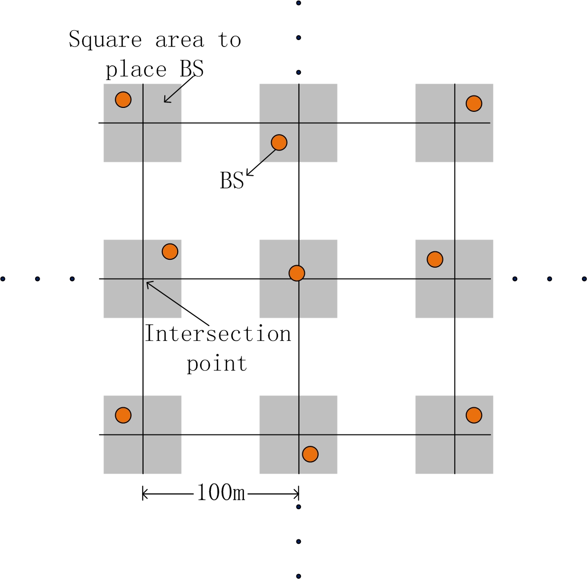
Figure 6: An illustration of BS placement in the C-DWN network considered in the simulations.

In this section, we illustrate the PHY caching gains for a general C-DWN network with 225 BSs and 900 users. The locations of the BSs and users are randomly generated according to Assumption 1 with parameters $r_{\textrm{min}}=50$m, $r_{\textrm{max}}=75\sqrt{2}$m, $d_{\textrm{min}}=10$m and $k_{\textrm{max}}=8$. Specifically, we first generate a $15\times 15$ grid as illustrated in Fig. 6. Then each BS is randomly placed in the square of side length $50$m (gray squares in Fig. 6) centered at each of the 225 intersection points on the gird. Finally, the users are placed one by one in the network. When placing the $k$-th user, we first randomly pick a cell that has less than $k_{\textrm{max}}=8$ users. Then, user $k$ is randomly placed at a point within the cell that is at least $d_{\textrm{min}}=10$m away from the BS in this cell. Only $N_{0}=10$ BSs have wired backhaul. The system bandwidth is 1MHz. There are $L=50$ content files on content server and the size of each file is 1GB. We assume Zipf popularity distribution with different values $\tau$. The BS cluster size in cache-induced Co-MIMO transmission is set as $N_{c}=9$.

In Fig. 7, we plot the per BS throughput versus the cache size $B_{C}$. The content popularity skewness $\tau$ is fixed as 1.5. It can be seen that both the cache-assisted multihopping gain and cache-induced MIMO cooperation gain increase with the cache size $B_{C}$, and both gains of PHY caching becomes significant when the BS cache size is large.

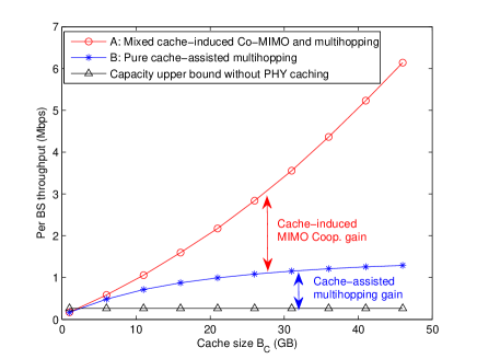
Figure 7: Per BS throughput versus the cache size $B_{C}$. The content popularity skewness $\tau$ is fixed as 1.5.

We then simulate the case when the BS cache size is much smaller than the total content size. In Fig. 8, we plot the per BS throughput versus the content popularity skewness $\tau$. The BS cache size is fixed as 5GB. The results in Fig. 8 show that both gains of PHY caching increase with the content popularity skewness $\tau$. Moreover, even when $B_{C}$ is small compared to the total content size, it is still possible to achieve a large PHY caching gain when $\tau$ is large, as shown in Fig. 8.

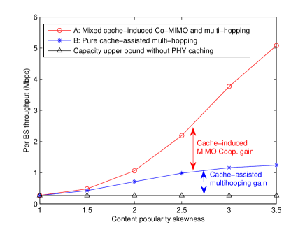
Figure 8: Per BS throughput versus the popularity skewness $\tau$. The BS cache size is fixed as 5GB and $L=50$.

VIII Discussion

In this section, we extend the results in this paper to study the impact of network deployment on the throughput scaling laws. Specifically, we consider the impact of two network parameters, namely the number of backhaul-connected BSs $N_{0}$ and the system loading in the network.

The number of backhaul-connected BSs $N_{0}$ controls the tradeoff between performance and deployment cost. In this paper, we focus on the backhaul-limited case when $N_{0}=\Theta\left(1\right)$. However, the results can be extended to the case with arbitrary $N_{0}\in\left[0,N\right]$. In this case, the achievable per user throughput scales according to $\Theta\left(\max\left\{R_{\textrm{BL}},\frac{N_{0}}{K}\right\}\right)$, where $R_{\textrm{BL}}$ is the achievable per user throughput when $N_{0}=\Theta\left(1\right)$ and its scaling law is described in Theorem 4, and $\frac{N_{0}}{K}$ is the contribution of the wired payload backhauls to the throughput scaling law. When $N_{0}=O\left(\frac{K}{\sqrt{LF/B_{C}}}\right)$, the number of wired payload backhauls is too small to affect the scaling law. However, as $N_{0}$ increases, the wired payload backhauls may contribute to the scaling law, depending on the popularity skewness $\tau$. For example, when the popularity skewness $1<\tau<3/2$ and $\Theta\left(N_{0}\right)>\Theta\left(\frac{B_{C}K}{FL^{3/2-\tau}}\right)$, the throughput scales according to $\Theta\left(\frac{N_{0}}{K}\right)$, which has order-wise improvement compared to $R_{\textrm{BL}}$. On the other hand, when $\tau>3/2$, the linear capacity scaling law can be achieved purely by PHY caching without any wired payload backhaul.

The system loading is another important network parameter that may affect the throughput scaling law. In practice, there are usually a large number of users within the coverage area of a network, but not all of them are active. For example, at peak hours, most of the users will be active, which corresponds to a large system loading, while at off-peak hours, the ratio of active users will be small, which corresponds to a light system loading. Hence, the system loading can be measured using the ratio of active users $\beta\in\left[0,1\right]$. In this paper, we focus on the more challenging case of full system loading (i.e., $\beta=1$), where all $K=\Theta\left(N\right)$ users are assumed to be active. However, the results can be extended to the case with arbitrary $\beta\in\left[0,1\right]$. In this case, the achievable per user throughput scales according to $\Theta\left(\min\left\{\frac{1}{\beta}R_{\textrm{BL}},1\right\}\right)$, where $R_{\textrm{BL}}$ is the achievable per user throughput under full system loading $\beta=1$ and its scaling law is described in Theorem 4. Hence, as $\beta$ decreases, the per user throughput will increase. However, when $\beta$ is order-wise smaller than a critical system loading $\beta_{0}=\Theta\left(R_{\textrm{BL}}\right)$, the order of the aggregate network throughput will degrade compared to the case when $\beta=1$. The critical system loading $\beta_{0}$ increases with both the cache size $B_{C}$ and popularity skewness $\tau$.

IX Conclusion

In this paper, we propose a PHY caching scheme to address the interference issue (via cache-induced opportunistic Co-MIMO) and the backhaul cost issue (via cache-assisted multihopping) in dense wireless networks. We establish the linear capacity scaling law and present order-optimal PHY caching and transmission schemes in the backhaul-limited C-DWN. We further study the impact of various system parameters on the PHY caching gain and provide fundamental design insight for the backhaul-limited C-DWN. Specifically, the analytical results show that the minimum cache size needed to achieve the linear capacity scaling and significant cache-induced MIMO cooperation gain decreases with the popularity skewness $\tau$, which measures the concentration of the popularity distribution. In practice, the popularity skewness $\tau$ can be large especially for mobile applications [29]. Hence both benefits of cache-assisted multihopping and cache-induced Co-MIMO provided by the PHY caching are very effective ways of enhancing the capacity of dense wireless networks.

-A Proof of Lemma 1 and Theorem 1

The throughput bound in (1) follows directly from the cut set bound. Using Assumption 1-1), it can be shown that both $\sum_{n^{{}^{\prime}}\notin\mathcal{B}_{P}}G^{b}\left(r_{n^{{}^{\prime}},n}^{b}\right)^{-\alpha}$ and $\sum_{k=1}^{K}G^{d}\left(r_{k,n}^{d}\right)^{-\alpha}$ can be bounded by some constant for all $n\in\mathcal{B}_{P}$. Hence, we have $\tilde{b}_{U}=\Theta\left(N_{0}\right)$. This completes the proof of Lemma 1.

The maximization problem in (1) is equivalent to:

$$\max_{\left\{x_{n}\left(\tilde{\mathbf{H}}\right)\right\}}\textrm{E}\left[\sum_{n=1}^{N_{0}}\log\left(1+y_{n}\left(\tilde{\mathbf{H}}\right)x_{n}\left(\tilde{\mathbf{H}}\right)\right)\right]$$ (12)

$$\textrm{s.t.}\>\textrm{E}\left[\sum_{n=1}^{N_{0}}x_{n}\left(\tilde{\mathbf{H}}\right)\right]\leq N_{0}P,$$

where $y_{n}\left(\tilde{\mathbf{H}}\right)$ is the $n$-th eigenvalue of $\tilde{\mathbf{H}}^{\dagger}\tilde{\mathbf{H}}$ and $x_{n}\left(\tilde{\mathbf{H}}\right)$ is the transmit power for the $n$-th eigenchannel. Since $\sum_{n=1}^{N_{0}}y_{n}\left(\tilde{\mathbf{H}}\right)=\textrm{Tr}\left(\tilde{\mathbf{H}}\tilde{\mathbf{H}}^{\dagger}\right)=\tilde{b}_{U},\forall\tilde{\mathbf{H}}$, the optimal objective value of (12) is upper bounded by that of

$$\max_{\left\{x_{n}\left(\tilde{\mathbf{H}}\right),y_{n}\left(\tilde{\mathbf{H}}\right)\right\}}\textrm{E}\left[\sum_{n=1}^{N_{0}}\log\left(1+y_{n}\left(\tilde{\mathbf{H}}\right)x_{n}\left(\tilde{\mathbf{H}}\right)\right)\right]$$ (13)

$$\textrm{s.t.}\>\textrm{E}\left[\sum_{n=1}^{N_{0}}x_{n}\left(\tilde{\mathbf{H}}\right)\right]\leq N_{0}P,\>\textrm{E}\left[\sum_{n=1}^{N_{0}}y_{n}\left(\tilde{\mathbf{H}}\right)\right]\leq\tilde{b}_{U},$$

where $y_{n}\left(\tilde{\mathbf{H}}\right)$ is also treat as an optimization variable. When $y_{n}\left(\tilde{\mathbf{H}}\right)$ is fixed as the $n$-th eigenvalue of $\tilde{\mathbf{H}}^{\dagger}\tilde{\mathbf{H}}$, problem (13) reduces to problem (12). It can be shown that the optimal objective value of (13) is equal to that of

$$\max_{\left\{x_{n}\left(\tilde{\mathbf{H}}\right)\right\}}\textrm{E}\left[\sum_{n=1}^{N_{0}}\log\left(1+\xi x_{n}^{2}\left(\tilde{\mathbf{H}}\right)\right)\right]$$ (14)

$$\textrm{s.t.}\>\textrm{E}\left[\sum_{n=1}^{N_{0}}x_{n}\left(\tilde{\mathbf{H}}\right)\right]\leq N_{0}P.$$

Since $f\left(\xi,x\right)$ is concave w.r.t. $x$ and $f\left(\xi,x\right)\geq\log\left(1+\xi x^{2}\right),\forall x\geq 0$, the optimal objective value of (14) is upper bounded by that of the following convex problem:

$$\max_{\left\{x_{n}\left(\tilde{\mathbf{H}}\right)\right\}}\textrm{E}\left[\sum_{n=1}^{N_{0}}f\left(\xi,x_{n}\left(\tilde{\mathbf{H}}\right)\right)\right]$$ (15)

$$\textrm{s.t.}\>\textrm{E}\left[\sum_{n=1}^{N_{0}}x_{n}\left(\tilde{\mathbf{H}}\right)\right]\leq N_{0}P.$$

By Jensen’s inequality, we have

$$\textrm{E}\left[\sum_{n=1}^{N_{0}}f\left(\xi,x_{n}\left(\tilde{\mathbf{H}}\right)\right)\right] \leq \sum_{n=1}^{N_{0}}f\left(\xi,\textrm{E}\left[x_{n}\left(\tilde{\mathbf{H}}\right)\right]\right)$$

$$\leq N_{0}f\left(\xi,\frac{1}{N_{0}}\textrm{E}\left[\sum_{n=1}^{N_{0}}x_{n}\left(\tilde{\mathbf{H}}\right)\right]\right).$$

Since $\textrm{E}\left[\sum_{n=1}^{N_{0}}x_{n}\left(\tilde{\mathbf{H}}\right)\right]\leq N_{0}P$, the optimal objective value of (15) is upper bounded by $N_{0}f\left(\xi,P\right)$. This completes the proof of Theorem 1.

-B Proof of Lemma 3-5

Proof of Lemma 3

Let $\mathcal{O}_{k}$ denote a disk centered at the BS $b_{k}$ with radius $r_{k}^{*}-r_{\textrm{max}}$ and let $\mathcal{O}_{k}^{{}^{\prime}}$ denote the intersection of $\mathcal{O}_{k}$ and the network coverage area (i.e., the square of area $Nr_{0}^{2}$). By Assumption 1-2), any point inside $\mathcal{O}_{k}^{{}^{\prime}}$ must lie in the coverage area of the BSs in $\overline{\mathcal{B}}_{k}$. Since the coverage area of each BS is less than $\pi r_{\textrm{max}}^{2}$, we must have $\mathcal{A}\left(\mathcal{O}_{k}^{{}^{\prime}}\right)\leq\left|\overline{\mathcal{B}}_{k}\right|\pi r_{\textrm{max}}^{2}$, where $\mathcal{A}\left(\mathcal{O}_{k}^{{}^{\prime}}\right)$ denotes the area of $\mathcal{O}_{k}^{{}^{\prime}}$. Since $\mathcal{A}\left(\mathcal{O}_{k}^{{}^{\prime}}\right)\geq\frac{\pi\left(r_{k}^{*}-r_{\textrm{max}}\right)^{2}}{4}$ and $\left|\overline{\mathcal{B}}_{k}\right|\leq\left\lceil 1/q_{l}\right\rceil-1$, we have $\frac{\pi\left(r_{k}^{*}-r_{\textrm{max}}\right)^{2}}{4}\leq\left(\left\lceil 1/q_{l}\right\rceil-1\right)\pi r_{\textrm{max}}^{2}$ and thus $r_{k}^{*}\leq\left(2\sqrt{\left\lceil 1/q_{l}\right\rceil-1}+1\right)r_{\textrm{max}}$.

Proof of Lemma 4

Construct a graph where the vertices are the BS nodes. There is an edge between any two BSs with distance no more than $r_{I}^{b}$. Then finding a frequency reuse scheme which satisfies Condition 1 is essentially a vertex coloring problem in graph theory. It is well known that a graph of degree no more than $D_{G}$ can have its vertices colored by using no more than $D_{G}+1$ colors, with no two neighboring vertices having the same color [31]. One can therefore allocate the cells with no more than $D_{G}+1$ subbands to satisfies Condition 1. The rest is to bound $D_{G}$, which is the number of BSs in a circle with radius $r_{I}^{b}$. Using Assumption 1-1), we must have $\frac{D_{G}\pi r_{\textrm{min}}^{2}}{4}\leq\pi\left(r_{I}^{b}+\frac{r_{\textrm{min}}}{2}\right)^{2}$.

Proof of Lemma 5

The routing line segments of a user $k$ can intersect cell $n$ only when the associated BS $b_{k}$ is within the radius $r_{k}^{*}$. By lemma 3, $r_{k}^{*}\leq\left(2\sqrt{\left\lceil 1/q_{l}\right\rceil-1}+1\right)r_{\textrm{max}}$ for any user $k$ requesting the $l$-th file. Let $n_{l}^{\textrm{max}}$ denote the maximum number of BSs in a circle with radius $\left(2\sqrt{\left\lceil 1/q_{l}\right\rceil-1}+1\right)r_{\textrm{max}}$. Then according to the above analysis, the average number of users whose routing line segments intersect cell $n$ is upper bounded by $\sum_{l}p_{l}n_{l}^{\textrm{max}}k_{\textrm{max}}$. Using similar analysis as for $D_{G}$, it can be shown that $n_{l}^{\textrm{max}}\leq\left(\frac{\left(4\sqrt{\left\lceil 1/q_{l}\right\rceil-1}+2\right)r_{\textrm{max}}}{r_{\textrm{min}}}+1\right)^{2}$. This completes the proof.

-C Proof of Theorem 5

Clearly, the throughput of each wireless inter-BS link $C_{b}=\Theta\left(1\right)$, and the per cell downlink access transmission rate $C_{d}=\Theta\left(1\right)$. Suppose we want to support a per user throughput of $R$. Then the traffic to be relayed by a BS due to wireless inter-BS transmission is upper bounded by $JR$ according to Lemma 5 and the traffic to be handled by a BS due to downlink access transmission is upper bounded by $k_{\textrm{max}}R$. Clearly, for a user requesting a file with multihop cache mode, a throughput of $R$ can be supported by Scheme A if no BS is overloaded, i.e., $JR\leq C_{b}$ and $k_{\textrm{max}}R\leq C_{d}$. Hence, a per user throughput of $R=\min\left(\frac{C_{b}}{J},\frac{C_{d}}{k_{\textrm{max}}}\right)$ is achievable. Since $J=\Theta\left(\sum_{l=1}^{L}p_{l}\sqrt{\frac{1}{q_{l}}}\right)$ from Lemma 5, the order of $R$ is given by (4). On the other hand, for a user requesting a file with Co-MIMO cache mode, it is clear that a throughput of $\Theta\left(1\right)\geq\Theta\left(\frac{1}{J}\right)$ is achievable. As a result, an overall per user throughput of $R=\Theta\left(\frac{1}{J}\right)$ is also achievable.

Consider the convex problem of maximizing the order of per user throughput:

$$\min_{\mathbf{q}}\sum_{l=1}^{L}p_{l}\sqrt{\frac{1}{q_{l}}},\>s.t.\>q_{l}\in\left[0,1\right],\forall l,\>\sum_{l=1}^{L}q_{l}\leq\frac{B_{C}}{F}.$$ (16)

By analyzing the KKT conditions, it can be shown that (5) is an order optimal solution for (16). By substituting (16) into $R=\Theta\left(1/\sum_{l=1}^{L}p_{l}\sqrt{\frac{1}{q_{l}}}\right)$, it can be verified that the order of $R$ is the same as that in Theorem 4.

-D Proof of Lemma 6

For each wireless inter-BS link, the bandwidth is $\frac{W_{b}}{36}$ (note that each BS has four wireless inter-BS links) and the transmit power on this bandwidth is $\frac{W_{b}P}{36W^{{}^{\prime}}}$. The noise power is $\frac{W_{b}\eta_{0}}{36}$ and it can be verified that the interference power is $\frac{W_{b}P}{36W^{{}^{\prime}}}G^{b}I_{R}\left(1,3\right)$. Hence the SINR of each wireless inter-BS link is $\frac{PG^{b}r_{0}^{-\alpha}}{W^{{}^{\prime}}\eta_{0}+PG^{b}I_{R}\left(1,3\right)}$ and the rate is given by $W_{b}R_{b}^{B}$.

Similarly, for downlink access transmission, the bandwidth allocated to each cell is $\frac{W_{d}}{4}$ and the transmit power on this bandwidth is $\frac{W_{d}P}{4W^{{}^{\prime}}}$. The noise power is $\frac{W_{d}\eta_{0}}{4}$ and it can be verified that the interference power is $\frac{W_{d}P}{4W^{{}^{\prime}}}G^{d}I_{R}\left(\frac{d_{0}}{r_{0}},2\right)$. Hence the SINR in downlink access transmission is $\frac{PG^{d}d_{0}^{-\alpha}}{W^{{}^{\prime}}\eta_{0}+PG^{d}I_{R}\left(\frac{d_{0}}{r_{0}},2\right)}$ and the per user average downlink access transmission rate is given by $W_{d}R_{d}^{B}$.

-E Proof of Theorem 7

Consider the dual uplink system [32] of the downlink system where in each cluster, the scheduled users act as the transmitters, the BSs act as the receivers, and the uplink channels are the Hermition of the corresponding downlink channels. We first study the per cluster throughput of the uplink system. Then the results can be transferred to the downlink system using the downlink-uplink duality [32]. At each time slot, the BS clusters are randomly formed and each cluster contains $N_{c}$ BSs in a square. Consider the following achievable scheme for the uplink system. In each cluster, the users whose distance from the cluster boundary is less than a threshold $d_{b}=\Theta\left(\left(N_{c}r_{0}\right)^{\frac{1}{2\left(\alpha-1\right)}}\right)$ is not allowed to transmit for interference control. The other $\overline{N}_{c}=\Theta\left(N_{c}-N_{c}^{\frac{\alpha}{2\left(\alpha-1\right)}}\right)$ scheduled users transmit at a constant power $P^{{}^{\prime}}=\frac{36W_{c}P}{4W_{b}+9W_{d}+36W_{c}}$. Consider a reference cluster. Treating the interference from other clusters as noise, we can achieve a per cluster throughput of

$$C_{u}=W_{c}\textrm{E}\left[\log\left|\mathbf{I}+P^{{}^{\prime}}\mathbf{\Omega}^{-1}\mathbf{H}_{c}\mathbf{H}_{c}^{\dagger}\right|\right],$$

where $\mathbf{H}_{c}=\left[h_{i,j}\right]_{i=1,...,N_{c},j=1,...,\overline{N}_{c}}\in\mathbb{C}^{N_{c}\times\overline{N}_{c}}$ and $h_{i,j}$ is the uplink channel between the $j$-th scheduled user and the $i$-th BS in the reference cluster, $\mathbf{\Omega}$ is the covariance of the inter-cluster interference plus noise at the BSs. Using Jensen’s inequality, we have

$$C_{u} \geq W_{c}\textrm{E}\left[\log\left|\mathbf{I}+P^{{}^{\prime}}\textrm{E}\left[\mathbf{\Omega}|\mathbf{H}_{c}\right]^{-1}\mathbf{H}_{c}\mathbf{H}_{c}^{\dagger}\right|\right]$$

$$= W_{c}\textrm{E}\left[\log\left|\mathbf{I}+\frac{P^{{}^{\prime}}}{W_{c}\eta_{0}+\Theta\left(Pd_{b}^{2-\alpha}\right)}\mathbf{H}_{c}\mathbf{H}_{c}^{\dagger}\right|\right]$$

$$= W_{c}\textrm{E}\left[\log\left|\mathbf{I}+\frac{P^{{}^{\prime}}}{W_{c}\eta_{0}}\mathbf{H}_{c}^{\dagger}\mathbf{H}_{c}\right|\right]+\Theta\left(PN_{c}^{\frac{\alpha}{2\left(\alpha-1\right)}}\right),$$

where the first equality follows from the fact that $\textrm{E}\left[\mathbf{\Omega}|\mathbf{H}_{c}\right]$ is diagonal and the nearest interfering user is at least $d_{b}$ away from the reference BSs.

We can use the same technique as in Appendix I of [13] to bound the term $\overline{C}_{u}\triangleq W_{c}\textrm{E}\left[\log\left|\mathbf{I}+\frac{P^{{}^{\prime}}}{W_{c}\eta_{0}}\mathbf{H}_{c}^{\dagger}\mathbf{H}_{c}\right|\right]$. Let $\lambda$ be chosen uniformly among the $\overline{N}_{c}$ eigenvalues of $\frac{\mathbf{H}_{c}^{\dagger}\mathbf{H}_{c}}{\overline{N}_{c}}$. Then

$$\overline{C}_{u} \geq W_{c}\overline{N}_{c}\textrm{E}\left[\log\left(1+\frac{\overline{N}_{c}P^{{}^{\prime}}}{W_{c}\eta_{0}}\lambda\right)\right]$$

$$\geq W_{c}\overline{N}_{c}\log\left(1+\frac{\overline{N}_{c}P^{{}^{\prime}}}{W_{c}\eta_{0}}t\right)\Pr\left(\lambda>t\right)$$

for any $t\geq 0$. By the Paley-Zygmund inequality, we have

$$\Pr\left(\lambda>t\right)\geq\frac{\left(\textrm{E}\left(\lambda\right)-t\right)^{2}}{\textrm{E}\left(\lambda^{2}\right)},\>0\leq t<\textrm{E}\left(\lambda\right).$$

Following similar analysis as in Appendix I of [13], we have

$$\textrm{E}\left(\lambda\right)=\frac{G^{d}}{\overline{N}_{c}^{2}}\sum_{k=1}^{\overline{N}_{c}}\sum_{i=1}^{N_{c}}r_{i,k}^{-\alpha}=\frac{G^{d}\left(G_{C}+O\left(N_{c}^{-\frac{\alpha-2}{2\left(\alpha-1\right)}}\right)\right)}{\overline{N}_{c}},$$

where the last equality follows from $\sum_{i=1}^{N_{c}}r_{i,k}^{-\alpha}=G_{C}+O\left(N_{c}^{-\frac{\alpha-2}{2\left(\alpha-1\right)}}\right)$, and

$$\textrm{E}\left(\lambda^{2}\right) = \frac{2\left(G^{d}\right)^{2}}{\overline{N}_{c}^{3}}\sum_{k=1}^{\overline{N}_{c}}\sum_{i=1}^{N_{c}}r_{i,k}^{-\alpha}\sum_{l=1}^{N_{c}}r_{l,k}^{-\alpha}$$

$$= \frac{2\left(G^{d}\right)^{2}\left(G_{C}+O\left(N_{c}^{-\frac{\alpha-2}{2\left(\alpha-1\right)}}\right)\right)^{2}}{\overline{N}_{c}^{2}}.$$

Choose $t=\frac{G^{d}d_{0}^{-\alpha}}{\overline{N}_{c}}$. We have

$$\overline{C}_{u}\geq W_{c}\overline{N}_{c}\rho\log\left(1+\frac{P^{{}^{\prime}}G^{d}d_{0}^{-\alpha}}{W_{c}\eta_{0}}\right)+O\left(PN_{c}^{\frac{\alpha}{2\left(\alpha-1\right)}}\right).$$

According to the downlink-uplink duality [32], a per cluster throughput of $C_{d}=C_{u}\geq\overline{C}_{u}+\Theta\left(PN_{c}^{\frac{\alpha}{2\left(\alpha-1\right)}}\right)$ can be achieved with equal or less total network power. Since the BS clusters are randomly formed, all users and BSs are statistically symmetric. As a result, the average downlink access transmission rate $R_{d}^{C^{\prime}}$ of a user on the Co-MIMO band is lower bounded as

$$R_{d}^{C^{\prime}} \geq \frac{C_{d}}{4N_{c}}$$

$$\geq \frac{\rho W_{c}}{4}\log\left(1+\frac{P^{{}^{\prime}}G^{d}d_{0}^{-\alpha}}{W_{c}\eta_{0}}\right)+\Theta\left(PN_{c}^{-\frac{\alpha-2}{2\left(\alpha-1\right)}}\right)$$

$$\geq \frac{\rho W_{c}}{4}\log\left(1+\frac{PG^{d}d_{0}^{-\alpha}}{W\eta_{0}}\right)+\Theta\left(PN_{c}^{-\frac{\alpha-2}{2\left(\alpha-1\right)}}\right)$$

and the average power at each BS required to achieve the above per user rate is no more than $P^{{}^{\prime}}$, where the last inequality follows from $\frac{P^{{}^{\prime}}}{W_{c}}=\frac{36P}{4W_{b}+9W_{d}+36W_{c}}\geq\frac{P}{W}$. On the other hand, using the cut set bound between all BSs and a user, we have

$$R_{d}^{C^{\prime}}\leq\frac{W_{c}}{4}\log\left(1+\frac{P^{{}^{\prime}}G^{d}G_{C}}{W_{c}\eta_{0}}\right)\overset{\textrm{a}}{\leq}W_{c}\log\left(1+\frac{9PG^{d}G_{C}}{W\eta_{0}}\right),$$ (17)

where (17-a) follows from $\frac{P^{{}^{\prime}}}{W_{c}}\leq\frac{9P}{W}$.

-F Proof of Theorem 6

First, we derive the maximum supportable per user throughput on the cache-assisted multihop band (i.e., inter-BS band plus downlink access band). Suppose the users request files $l\in\Omega\left(\mathbf{q}\right)$ at per user throughput $R$ on the cache-assisted multihop band. Let us focus on a reference user $k$. According to the proposed source BS set selection scheme, for each requested file segment, $q_{l}L_{S}$ parity bits are obtained from the associated BS, a total number of $4mq_{l}L_{S}$ parity bits are obtained from the source BSs in $\mathcal{B}_{k,m}$ for $1\leq m<\phi\left(q_{l}\right)$, and a total number of $\left(1-\left(1+2\phi^{2}\left(q_{l}\right)-2\phi\left(q_{l}\right)\right)q_{l}\right)L_{S}$ parity bits are obtained from the source BSs in $\mathcal{B}_{k,\phi\left(q_{l}\right)}$. As a result, the wireless inter-BS traffic $T_{l}$ induced by a single user requesting the $l$-th file is

$$T_{l} = \sum_{m=1}^{\phi\left(q_{l}\right)-1}4m^{2}q_{l}R+$$

$$\phi\left(q_{l}\right)\left(1-\left(1+2\phi^{2}\left(q_{l}\right)-2\phi\left(q_{l}\right)\right)q_{l}\right)R$$

$$= \left(\phi\left(q_{l}\right)\left(1-q_{l}\right)-\frac{2}{3}(\phi^{3}\left(q_{l}\right)-\phi\left(q_{l}\right))q_{l}\right)R.$$

Note that the ratio between the number of wireless inter-BS links and the number of users is $\lim_{N\rightarrow\infty}\frac{4N-4\sqrt{N}}{4N}=1$. Since all wireless inter-BS links are symmetric, the total wireless inter-BS traffic induced by all users are equally partitioned among all wireless inter-BS links. Hence, the corresponding traffic on each wireless inter-BS link is $\sum_{l\in\Omega\left(\mathbf{q}\right)}p_{l}T_{l}/Q_{\mathbf{q}}^{d}$ and we must have $\sum_{l\in\Omega\left(\mathbf{q}\right)}p_{l}T_{l}/Q_{\mathbf{q}}^{d}\leq W_{b}R_{b}\left(W_{b},W_{c}\right)$. Meanwhile. we have $R\leq\left(W-W_{b}-W_{c}\right)R_{d}\left(W_{b},W_{c}\right)$. Hence, the maximum supportable per user throughput on the cache-assisted multihop band $R_{m}\left(W_{b},W_{c}\right)=\min\left(\frac{Q_{\mathbf{q}}^{d}W_{b}R_{b}\left(W_{b},W_{c}\right)}{Q_{\mathbf{q}}^{b}},\left(W-W_{b}-W_{c}\right)R_{d}\left(W_{b},W_{c}\right)\right)$. On the other hand, it is easy to see that the maximum supportable per user throughput on the Co-MIMO band is $W_{c}R_{c}\left(W_{b},W_{c}\right)$.

The overall per user throughput is defined as $T_{\mathbf{q}}\left(W_{b},W_{c}\right)=\lim_{L_{0}\rightarrow\infty}\frac{L_{0}F}{t_{0}}$, where $L_{0}$ is the total number files delivered to a reference user $k$ within time $t_{0}$. Let $L_{l}$ denote the number of delivering the $l$-th file. Clearly, we have

$$\lim_{L_{0}\rightarrow\infty}t_{0}=\max\left(\frac{\sum_{l\in\Omega\left(\mathbf{q}\right)}FL_{l}}{R_{m}\left(W_{b},W_{c}\right)},\frac{\sum_{l\in\overline{\Omega}\left(\mathbf{q}\right)}FL_{l}}{W_{c}R_{c}\left(W_{b},W_{c}\right)}\right)$$

$$T_{\mathbf{q}}\left(W_{b},W_{c}\right) = \lim_{L_{0}\rightarrow\infty}\frac{L_{0}F}{\max\left(\frac{\sum_{l\in\Omega\left(\mathbf{q}\right)}FL_{l}}{R_{m}\left(W_{b},W_{c}\right)},\frac{\sum_{l\in\overline{\Omega}\left(\mathbf{q}\right)}FL_{l}}{W_{c}R_{c}\left(W_{b},W_{c}\right)}\right)}$$

$$= \lim_{L_{0}\rightarrow\infty}\frac{1}{\max\left(\frac{Q_{\mathbf{q}}^{d}}{R_{m}\left(W_{b},W_{c}\right)},\frac{Q_{\mathbf{q}}^{c}}{W_{c}R_{c}\left(W_{b},W_{c}\right)}\right)},$$

where the last equality follows from $\lim_{L_{0}\rightarrow\infty}\frac{L_{l}}{L_{0}}=p_{l}$. Clearly, $T_{\mathbf{q}}^{L}\left(W_{b},W_{c}\right)+O\left(PN_{c}^{-\frac{\alpha-2}{2\left(\alpha-1\right)}}\right)\leq T_{\mathbf{q}}\left(W_{b},W_{c}\right)\leq T_{\mathbf{q}}^{U}\left(W_{b},W_{c}\right)$, where $T_{\mathbf{q}}^{a}\left(W_{b},W_{c}\right)$ is obtained by replacing $R_{b}\left(W_{b},W_{c}\right),R_{d}\left(W_{b},W_{c}\right),R_{c}\left(W_{b},W_{c}\right)$ in $T_{\mathbf{q}}\left(W_{b},W_{c}\right)$ with $R_{b}^{a},R_{d}^{a},R_{c}^{a}$ for $a\in\left\{U,L\right\}$. Hence, the per BS throughput $\Gamma_{A}\left(\mathbf{q}\right)$ is bounded as $\Gamma_{A}^{U}\left(\mathbf{q}\right)\geq\Gamma_{A}\left(\mathbf{q}\right)\geq\Gamma_{A}^{L}\left(\mathbf{q}\right)+O\left(PN_{c}^{-\frac{\alpha-2}{2\left(\alpha-1\right)}}\right)$ with $\Gamma_{A}^{a}\left(\mathbf{q}\right)\triangleq\max_{W_{b},W_{c}\in\left(0,W\right)}4T_{\mathbf{q}}^{a}\left(W_{b},W_{c}\right)$ for $a\in\left\{U,L\right\}$. It can be verified that $\Gamma_{A}^{a}\left(\mathbf{q}\right)$ is given in (6). Finally, as $P,N_{c}\rightarrow\infty$ such that $PN_{c}^{-\frac{\alpha-2}{2\left(\alpha-1\right)}}\rightarrow 0$, we have $R_{b}^{a}\rightarrow\frac{1}{36}\tilde{R}_{b}$, $R_{d}^{a}\rightarrow\frac{1}{16}\tilde{R}_{d},$ $R_{b}^{a}/R_{c}^{a}\rightarrow 0$, and $R_{d}^{a}/R_{c}^{a}\rightarrow 0$ for $a\in\left\{L,U\right\}$, from which (8) follows.

References

- [1] H. Zhang and H. Dai, “Cochannel interference mitigation and cooperative processing in downlink multicell multiuser MIMO networks,” EURASIP Journal on Wireless Communications and Networking, vol. 2004, no. 2, pp. 222–235, 2004.
- [2] O. Somekh, O. Simeone, Y. Bar-Ness, A. Haimovich, and S. Shamai, “Cooperative multicell zero-forcing beamforming in cellular downlink channels,” IEEE Trans. Inf. Theory, vol. 55, no. 7, pp. 3206–3219, 2009.
- [3] R. Irmer, H. Droste, P. Marsch, M. Grieger, G. Fettweis, S. Brueck, H.-P. Mayer, L. Thiele, and V. Jungnickel, “Coordinated multipoint: Concepts, performance, and field trial results,” IEEE Communications Magazine, vol. 49, no. 2, pp. 102 –111, Feb. 2011.
- [4] M. Paolini, “Crucial economics for mobile data backhaul,” Senza Fili Consulting, 2011. [Online]. Available: http://smallcells.com/SenzaFiliBackhaulTCO.pdf
- [5] N. Golrezaei, K. Shanmugam, A. Dimakis, A. Molisch, and G. Caire, “Femtocaching: Wireless video content delivery through distributed caching helpers,” in Proc. IEEE INFOCOM, pp. 1107–1115, 2012.
- [6] Y. Shi, M. Li, X. Xiong, and G. Han, “A flexible wireless backhaul solution for emerging small cells networks,” in Proc. IEEE ICSPCC 2014, Aug. 2014, pp. 591–596.
- [7] X. Ge, H. Cheng, M. Guizani, and T. Han, “5G wireless backhaul networks: challenges and research advances,” IEEE Network, vol. 28, no. 6, pp. 6–11, Nov. 2014.
- [8] M. C. et al., “Wireless backhaul in future heterogeneous networks,” Ericsson Rev., vol. 91, Nov. 2014.
- [9] P. Gupta and P. Kumar, “The capacity of wireless networks,” IEEE Trans. Info. Theory, vol. 46, no. 2, pp. 388–404, Mar 2000.
- [10] X. Liang-Liang and P. R. Kumar, “A network information theory for wireless communication: scaling laws and optimal operation,” IEEE Trans. Info. Theory, vol. 50, no. 5, pp. 748–767, 2004.
- [11] A. Jovicic, P. Viswanath, and S. Kulkarni, “Upper bounds to transport capacity of wireless networks,” IEEE Trans. Info. Theory, vol. 50, no. 11, pp. 2555–2565, Nov 2004.
- [12] L.-L. Xie and P. Kumar, “On the path-loss attenuation regime for positive cost and linear scaling of transport capacity in wireless networks,” IEEE Trans. Info. Theory, vol. 52, no. 6, pp. 2313–2328, June 2006.
- [13] A. Ozgur, O. Leveque, and D. Tse, “Hierarchical cooperation achieves optimal capacity scaling in ad hoc networks,” IEEE Trans. Info. Theory, vol. 53, no. 10, pp. 3549–3572, Oct 2007.
- [14] U. Niesen, P. Gupta, and D. Shah, “On capacity scaling in arbitrary wireless networks,” IEEE Trans. Info. Theory, vol. 55, no. 9, pp. 3959–3982, Sept 2009.
- [15] ——, “The balanced unicast and multicast capacity regions of large wireless networks,” IEEE Trans. Info. Theory, vol. 56, no. 5, pp. 2249–2271, May 2010.
- [16] P. Li, X. Huang, and Y. Fang, “Capacity scaling of multihop cellular networks,” in Proc. IEEE INFOCOM 2011, Apr. 2011, pp. 2831–2839.
- [17] S. Goebbels, “Disruption tolerant networking by smart caching,” Int. J. Commun. Syst., vol. 23, no. 5, pp. 569–595, May 2010.
- [18] M. Maddah-Ali and U. Niesen, “Fundamental limits of caching,” IEEE Trans. Info. Theory, vol. 60, no. 5, pp. 2856–2867, May 2014.
- [19] E. Bastug, M. Bennis, and M. Debbah, “Living on the edge: The role of proactive caching in 5G wireless networks,” IEEE Communications Magazine, vol. 52, no. 8, pp. 82–89, Aug 2014.
- [20] M. Ji, G. Caire, and A. Molisch, “Fundamental limits of distributed caching in D2D wireless networks,” 2013. [Online]. Available: http://arxiv.org/abs/1304.5856
- [21] M. Ji, G. Caire, and A. F. Molisch, “The throughput-outage tradeoff of wireless one-hop caching networks,” 2013. [Online]. Available: http://arxiv.org/abs/1312.2637
- [22] A. Altieri, P. Piantanida, L. R. Vega, and C. G. Galarza, “On fundamental trade-offs of device-to-device communications in large wireless networks,” IEEE Trans. Wireless Commun., vol. 14, no. 9, pp. 4958–4971, Sept 2015.
- [23] S.-W. Jeon, S.-N. Hong, M. Ji, and G. Caire, “Caching in wireless multihop device-to-device networks,” in Proc. IEEE ICC 2015, June 2015, pp. 6732–6737.
- [24] S. Gitzenis, G. Paschos, and L. Tassiulas, “Asymptotic laws for joint content replication and delivery in wireless networks,” IEEE Trans. Info. Theory, vol. 59, no. 5, pp. 2760–2776, May 2013.
- [25] A. Liu and V. Lau, “Cache-enabled opportunistic cooperative MIMO for video streaming in wireless systems,” IEEE Trans. Signal Processing, vol. 62, no. 2, pp. 390–402, Jan 2014.
- [26] ——, “Mixed-timescale precoding and cache control in cached MIMO interference network,” IEEE Trans. Signal Processing, vol. 61, no. 24, pp. 6320–6332, Dec 2013.
- [27] ——, “Asymptotic scaling laws of wireless adhoc network with physical layer caching,” accepted by IEEE Trans. Wireless Commun., 2015. [Online]. Available: http://arxiv.org/abs/1510.05205
- [28] M. Ji, G. Caire, and A. F. Molisch, “Wireless device-to-device caching networks: Basic principles and system performance,” IEEE J. Select. Areas Commun., vol. 34, no. 1, pp. 176–189, Jan 2016.
- [29] T. Yamakami, “A zipf-like distribution of popularity and hits in the mobile web pages with short life time,” in Proc. Parallel Distrib. Comput., Appl. Technol., Taipei, Taiwan, Dec 2006, pp. 240–243.
- [30] A. Shokrollahi, “Raptor codes,” IEEE Trans. Info. Theory, vol. 52, no. 6, pp. 2551–2567, 2006.
- [31] J. A. Bondy and U. Murthy, Graph Theory with Applications. New York: Elsevier, 1976.
- [32] A. Liu, Y. Liu, H. Xiang, and W. Luo, “MIMO B-MAC interference network optimization under rate constraints by polite water-filling and duality,” IEEE Trans. Signal Processing, vol. 59, no. 1, pp. 263 –276, Jan. 2011.