Chaos and Stochastic Models in Physics: Ontic and Epistemic Aspects


Sergio Caprara and Angelo Vulpiani

Dipartimento di Fisica - Università Sapienza, Roma


Abstract There is a persistent confusion about determinism and predictability. In spite of the opinions of some eminent philosophers (e.g., Popper), it is possible to understand that the two concepts are completely unrelated. In few words we can say that determinism is ontic and has to do with how Nature behaves, while predictability is epistemic and is related to what the human beings are able to compute. An analysis of the Lyapunov exponents and the Kolmogorov-Sinai entropy shows how deterministic chaos, although with an epistemic character, is non subjective at all. This should clarify the role and content of stochastic models in the description of the physical world.

1 Introduction

In the last decades scientists and philosophers showed an intense interest for chaos, chance and predictability. Some aspects of such topics are rather subtle, and in the literature is not unusual to find wrong statements. In particular it is important to avoid confusion on the fact that to be deterministic (or stochastic) is an ontic property of a system, i.e. related to its own nature independently of our knowledge; while predictability, and somehow chaos, have an epistemic character, i.e. depend on our knowledge. We will see how the introduction of a probabilistic approach in deterministic chaotic systems, although with an epistemic character, is not subjective.

Often in the past, the central goal of science has been though to be “prediction and control”, we can mention von Neumann’s belief that powerful computers and a clever use of numerical analysis would eventually lead to accurate forecasts, and even to the control, of weather and climate:

The computer will enable us to divide the atmosphere at any moment into stable regions and unstable regions. Stable regions we can predict. Unstable regions we can control.

The great scientist von Neumann was wrong, but he did not know the phenomenon of deterministic chaos.

About half a century ago, thanks to the contribution of M. Hénon, E. Lorenz and B. V. Chirikov (to cite just some of the most eminent scientists in the field), deterministic chaos was (re)discovered. Such an event sure was scientifically important, e.g., as it clarifies topics like the different possible origins of the statistical laws and the intrinsic practical limits of the predictions. On the other hand, one has to admit that the term “deterministic chaos” can be seen as an oxymoron and induced the persistence of a certain confusion about concepts as determinism, predictability and stochastic laws. Our aim is to try to put some order into this matter, discussing some aspects of deterministic chaos which, in our opinion, are often misunderstood, leading to scientifically, as well as philosophically, questionable and confused claims.

In spite of the fact that it is quite evident that Maxwell, Duhem, and Poincaré understood in a clear way the distinction between determinism and chaos, in the recent literature one can find a large spectrum of wrong statements on the conceptual impact of deterministic chaos, see Campbell and Garnett (1882). For instance, Prigogine and Stengers (1994) claim that the notion of chaos leads us to rethink the notion of “law of nature”. In a book on statistical physics (Vauclair 1993), one can read that as consequence of chaos the deterministic approach fails. Sir James Lightill (1986) in a lecture to the Royal Society on the 300th anniversary of Newton’s Principia shows how to confuse determinism and prediction: We are all deeply conscious today that the enthusiasm of our forebears for the marvelous achievements of Newtonian mechanics led them to make generalization in this area of predictability, which indeed we may generally have tended to believe before 1960, but which we now recognize were false. We collectively wish to apologize for having misled the generally educated public by spreading ideas about the determinism of systems satisfying Newton’s laws of motion, that after 1960 were to be proved incorrect.

Chaos presents both ontic and epistemic aspects which may generate confusion about the real conceptual relevance of chaos. We shall see that chaos allows us to unambiguously introduce probabilistic concepts in a deterministic world. Such a possibility is not merely the consequence of our limited knowledge of the state of the system of interest. Indeed, in order to account for this limited knowledge, one usually relies on a coarse-grained description, which requires a probabilistic approach. We will see that many important features of the dynamics do not depend on the scale $\epsilon$ of the graining, if it is fine enough. At the same time, many results for the $\epsilon\to 0$ limit do not apply to the cases with $\epsilon=0$. Therefore, the probabilistic description of chaotic systems reveals one more instance of singular limits.

2 About determinism

The word determinism has often been used in fields other than physics, such as psychology and sociology, causing some bewilderment. There have been some misunderstandings about the meaning of determinism, and because, at times, determinism has been improperly associated with reductionism, mechanicism and predictability (Chibbaro, et al. 2014), it seems to us that a brief review of the notion of determinism is not useless.

For example, unlike the majority of modern physicists and mathematicians, by deterministic system Popper (1992) means a system governed by a deterministic evolution law, whose evolution can be in principle predicted with arbitrary accuracy:

Scientific determinism is the doctrine that the state of any closed physical system at any future instant can be predicted.

In other words, Popper confuses determinism and prediction.

On the contrary, Russell gives the following definition, which is in agreement with the present mathematical terminology:

A system is said to be “deterministic” when, given certain data $e_{1},e_{2},...,e_{n}$ at times $t_{1},t_{2},...,t_{n}$, respectively, concerning this system, if $E_{t}$ is the state of the system at any (later) time $t$, there is a functional relation of the form

$$E_{t}=f(e_{1},t_{1},e_{2},t_{2},...,e_{n},t_{n})\,.$$

In the definition of Russell practical prediction is not mentioned.

The confusion about determinism and predictability is not isolated, see, e.g., Stone (1989) and Boyd (1972) who examine in great detail arguments about the widespread opinion that human behavior is not deterministic because it is not predictable.

Determinism amounts to the metaphysical doctrine that same events always follow from same antecedents. But, as Maxwell had already pointed out in 1873, it is impossible to confirm this fact, because nobody has ever experienced the same situation twice:

It is a metaphysical doctrine that from the same antecedents follow the same consequences. No one can gainsay this. But it is not of much use in a world like this, in which the same antecedents never again concur, and nothing ever happens twice … The physical axiom which has a somewhat similar aspect is “that from like antecedents follow like consequences”. But here we have passed … from absolute accuracy to a more or less rough approximation.

In these few lines, Maxwell touches on issues which will be later investigated, and anticipates their solution. The issues are:

1. the impossibility of proving (or refuting) the deterministic character of the laws of Nature;

2. the practical impossibility of making long-term predictions for a class of phenomena, referred to here as chaotic, despite their deterministic nature.

After the development of quantum mechanics, many think that discussing the deterministic nature of the laws of physics is too academic an exercise to deserve serious consideration. For instance, in a speech motivated by the heated controversy on chaos and determinism between philosophers and scientists, Kampen (1991) bluntly said that the problem does not exist, as it is possible to show that:

the ontological determinism à la Laplace can neither be proved nor disproved on the basis of observations.

It is not difficult to realize that determinism and predictability constitute two quite distinct issues, and the former does not imply the latter. Roughly speaking, determinism can be traced back to a vision of the nature of causality and can be cast in mathematical terms, by saying that the laws of nature are expressed by ordinary (or partial) differential equations. However, as noted by Maxwell, the objectively ontological determinism of the laws of nature cannot be proven; but one might find it convenient to use deterministic descriptions. Moreover, even at a macroscopic level, many phenomena are chaotic and, in some sense, appear to be “random”. On the other hand, the microscopic phenomena described by quantum mechanics, fall directly within a probabilistic framework. When referring to observable properties, they appear ontologically and epistemologically non-deterministic.

3 Two explicit examples

In order to clarify the concepts of determinism, predictability and chaos let us discuss two deterministic systems whose behaviors are rather different. They do not have particular own relevance, their choice is motivated just for pedagogical reasons:
Example A The pendulum (of length $L$):

$${d^{2}\theta\over dt^{2}}=-{g\over L}\sin\theta\,.$$

According to well known mathematical theorems on differential equations the following results hold:
a) the initial condition $(\theta(0),d\theta(0)/dt)$ determines in a unique way the state of the system $(\theta(t),d\theta(t)/dt)$ at any time $t$, in other words the system is deterministic;
b) the motion is periodic, i.e., there exists a time $T$ (depending on the initial conditions) such that

$$\Big{(}\theta(t+T),{d\theta(t+T)\over dt}\Big{)}=\Big{(}\theta(t),{d\theta(t)\over dt}\Big{)}\,;$$

c) the time evolution can be expressed via a function $F(t,\theta(0),d\theta(0)/dt)$:

$$\theta(t)=F\Big{(}t,\theta(0),{d\theta(0)\over dt}\Big{)}\,.$$

The function $F$ can be explicitly written only if $\theta(0)$ and $d\theta(0)/dt$ are small (and, in such a case, $T=2\pi\sqrt{L/g}$ is a constant, independent of the initial conditions); however, in the generic case, $F$ can be easily determined with the desired precision.

Example B Bernoulli’s shift:

$$x_{t+1}=2x_{t}\,\,\,mod\,\,1\,.$$

Where the operation $mod\,\,1$ corresponds to taking the fractional part of a number, e.g., $1.473\,\,mod\,\,1=0.473$. It is easy to understand that the above system is deterministic: $x_{0}$ determines $x_{1}$, which determines $x_{2}$ and so on. Let us show that the above system is chaotic: a small error in the initial conditions doubles at every step. Suppose that $x_{0}$ is a real number in the interval $[0,1]$, it can be expressed by an infinite sequence of $0$ and $1$:

$$x_{0}={a_{1}\over 2}+{a_{2}\over 4}+...+{a_{n}\over 2^{n}}+...,$$

where every $a_{n}$ takes either the value $0$ or the value $1$. The above binary notation allows us to determine the time evolution by means of a very simple rule: at every step, one has just move the “binary point” of the binary expansion of $x_{0}$ by one position to the right and eliminate the integer part. For example, take

$$x_{0}=0.11010000101110101010101100.....$$

$$x_{1}=0.1010000101110101010101100.......$$

$$x_{2}=0.010000101110101010101100.........$$

$$x_{3}=0.10000101110101010101100...........$$

and so on. In terms of the sequence $\{a_{1},a_{2},...\}$, it becomes quite clear how crucially the temporal evolution depends on the initial condition. Let us consider two initial conditions $x^{(1)}_{0}$ and $x^{(2)}_{0}$ such that $|x^{(1)}_{0}-x^{(2)}_{0}|<2^{-M}$ for some arbitrary (large) integer number $M$, this means that $x^{(1)}_{0}$ and $x^{(2)}_{0}$ have the first $M$ binary digits identical, and they may differ only afterwards. The above discussion shows that the distance between the points increases rapidly: for $t<M$ one has an exponential growth of the distance between the two trajectories

$$|x^{(1)}_{t}-x^{(2)}_{t}|\sim|x^{(1)}_{0}-x^{(2)}_{0}|\,2^{t}\,.$$

As soon as $t>M$, one can only conclude that $|x^{(1)}_{t}-x^{(2)}_{t}|<1$. Our system is chaotic: even an arbitrarily small error in the initial conditions eventually dominates the dynamics of the system, making long-term prediction impossible.

From the above discussion we saw how in deterministic systems one can have the following possible cases (in decreasing order of predictability):
I- Explicit possibility to determine the future (pendulum in the limit of small oscillations);
II- Good control of the prediction, without an explicit solution (pendulum with large oscillations);
III- Chaos and practical impossibility of predictability (Bernoulli’s shift).

3.1 About the ontic/epistemic character of chaos

One should also beware of the possible confusion between ontic and epistemic descriptions, when studying the topic of chaos. Determinism simply means that: given the same initial state ${\bf X}(0)$, one always finds the same evolved state ${\bf X}(t)$, at any later time $t>0$. Therefore, determinism refers exclusively to ontic descriptions, and it does not deal with prediction. This has been clearly stressed by Atmanspacher (2002), in a paper by the rather eloquent title Determinism is ontic, determinability is epistemic. This distinction between ontic and epistemic descriptions was obvious to Maxwell; after having noted the metaphysical nature of the problem of determinism in physics, he stated that:

There are certain classes of phenomena … in which a small error in the data only introduces a small error in the result … There are other classes of phenomena which are more complicated, and in which cases of instability may occur.

Also for Poincaré the distinction between determinism and prediction was rather clear, on the contrary, Popper (1992) confused determinism and prediction.

4 Chaos and asymptotics

Here, we briefly recall the essential properties of a deterministic chaotic system:
I- The evolution is given by a deterministic rule, for example, by a set of differential equations;
II- Solutions sensitively depend on the initial conditions: i.e., two initially almost identical states ${\bf X}(0)$ and ${\bf X}^{\prime}(0)$, with a very small initial displacement $|{\bf X}^{\prime}(0)-{\bf X}(0)|=\delta_{0}$, become separated at an exponential rate:

$$|{\bf X}^{\prime}(t)-{\bf X}(t)|=\delta_{t}\sim\delta_{0}\,e^{\lambda t}\,,$$

where $\lambda$ is positive and is called the Lyapunov exponent, for Bernoulli’s shift $\lambda=\ln 2$;
III- The evolution of the state ${\bf X}(t)$ is not periodic and appears quite irregular, similar in many respects to that of random systems.

The sensitive dependence on the initial condition drastically limits the possibility of making predictions: if the initial state is known with a certain uncertainty $\delta_{0}$, the evolution of the system can be accurately predicted with precision $\Delta$ only up to a time that depends on the Lyapunov exponent. This quantity is inherent in the system and does not depend on our ability to determine the initial state; hence, recalling Eq. (3), the time within which the error on the prediction does not exceed the desired tolerance is:

$$T_{p}\sim{1\over\lambda}\ln{\Delta\over\delta_{0}}\,.$$

The sensitivity to initial conditions introduces an error in predictions which grows exponentially in time. As the Lyapunov exponent $\lambda$ is an intrinsic characteristic of the system, predictions remain meaningful only within a time given by Eq. (4); therefore, it is well evident that a deterministic nature does not imply the possibility of an arbitrarily accurate prediction.

Let us note that, since ${\bf X}$ is in a bounded domain, some accuracy is needed in the definition of the Lyapunov exponent: before one has to take the limit $\delta_{0}\to 0$ and then $t\to\infty$:

$$\lambda=\lim_{t\to\infty}\lim_{\delta_{0}\to 0}{1\over t}\ln\Big{(}{\delta_{t}\over\delta_{0}}\Big{)}\,.$$

Another important characterisation of the dynamics is given by the Kolmogorov-Sinai entropy, $h_{KS}$, defined as follows. Just for the sake of simplicity we consider a system with discrete time: let ${\cal A}=\{A_{1},...,A_{N}\}$ be a finite partition of the phase space (the space of configurations of a given system under study), made up of the $N$ disjoint sets $A_{i}$, and consider the sequence of points

$$\{{\bf x}_{1},...,{\bf x}_{n},...\}\,,$$

which constitutes the trajectory with initial condition ${\bf x}_{0}$. This trajectory can be associated with the symbol sequence

$$\{i_{0},i_{1},...,i_{n},...\}\,,$$

where $i_{k}=j$ if ${\bf x}_{k}\in A_{j}$.

Once a partition ${\cal A}$ has been introduced, the coarse-grained properties of chaotic trajectories can be therefore studied through the discrete time sequence (5). Let $C_{m}=(i_{1},i_{2},...i_{m})$ be a “word” (a string of symbols) of length $m$ and probability $P(C_{m})$. The quantity

$$H_{m}=\sum_{C_{m}}P(C_{m})\ln P(C_{m})$$

is called the block entropy of the $m$-sequences. In the limit of infinitely long sequences, the asymptotic entropy increment

$$h_{S}({\cal A})=\lim_{m\to\infty}(H_{m+1}-H_{m})$$

is called the Shannon entropy, and in general depends on the partition ${\cal A}$ . Taking the largest value over all possible partitions we obtain the so-called Kolmogorov-Sinai entropy:

$$h_{KS}=\sup_{{\cal A}}h_{S}({\cal A})\,.$$

A more intuitive definition of $h_{KS}$ starts from the partition ${\cal A}_{\epsilon}$ made of a grid of hypercubes with sides of length $\epsilon$, and takes the following limit:

$$h_{KS}=\lim_{\epsilon\to 0}h(\epsilon)\,,$$

where $h(\epsilon)=h_{S}({\cal A}_{\epsilon})$.

Naively, one might consider chaos in deterministic systems to be illusory, just a consequence of our observational limitations. Apparently, such a conclusion is confirmed by the fact that important measures of the dynamical complexity, such as the Lyapunov exponent $\lambda$ and the Kolmogorov-Sinai entropy $h_{KS}$, are defined via finite, albeit arbitrarily high, resolutions. For instance, in the computation of $\lambda$ one considers two trajectories, which are initially very close $|{\bf X}(0)-{\bf X}^{\prime}(0)|=\delta_{0}$ and diverge in time from each other. Similarly, $h_{KS}$ is computed introducing a partition of the phase space, whose elementary cells have a finite size $\epsilon$. However, in the small-$\epsilon$ limit, $h(\epsilon)$ asymptotically tends to a value ($h_{KS}$) that no longer depends on $\epsilon$, as happens to $\lambda$ in the small-$\delta_{0}$ limit. Therefore, $\lambda$ and $h_{KS}$ can be considered intrinsic properties of the dynamics themselves: they do not depend on our observational ability, provided it is finite, i.e., provided $\epsilon$ and $\delta_{0}$ do not vanish.
According to Primas (2002), measures of stability, such as the Lyapunov exponent, concern ontic descriptions, whereas measures of information content or information loss, such as the Kolmogorov-Sinai entropy, relate to epistemic descriptions. We agree as far as stability is concerned. Regarding the epistemic character of $h_{KS}$, we observe that the Shannon entropy of a sequence of data, as well as the Kolmogorov-Sinai entropy, enjoy an epistemic status from a certain viewpoint, but not from another. The epistemic status arises from the fact that information theory deals with transmission and reception of data, which is necessarily finite. On the other hand, $h_{KS}$ is definitely an objective quantity, which does not depend on our observational limitations, as demonstrated by the fact that it can be expressed in terms of Lyapunov exponents (Cencini, et al. 2009). We note that the $\epsilon$-entropy $h(\epsilon)$ can be introduced even for stochastic processes, therefore it is a concept which links deterministic and stochastic descriptions.

5 Chaos and probability

After the (re)discovery of chaos in deterministic systems, owing to the presence of irregular and unpredictable behaviours, it is quite natural to adopt a probabilistic approach even in the deterministic realm. Let us assume that we known the probability density of configurations in phase space at the initial time $\rho({\bf x},0)$, it is possible to write down its time evolution law:

$$\rho({\bf x},0)\to\rho({\bf x},t)\,.$$

Under certain conditions (mixing) one has that al large time the probability density approaches a function which does not depend on $\rho({\bf x},0)$:

$$\lim_{t\to\infty}\rho({\bf x},t)=\rho^{inv}({\bf x})\,,$$

and is therefore called the invariant probability density. For instance, for Bernoulli’s shift one has the following recursive rule:

$$\rho(x,t+1)={1\over 2}\rho\left({x\over 2},t\right)+{1\over 2}\rho\left({x\over 2}+{1\over 2},t\right)\,,$$

and the invariant probability density is constant in the interval $[0,1]$:

$$\lim_{t\to\infty}\rho(x,t)=\rho^{inv}(x)=1\,.$$

It is rather natural, from an epistemic point of view, to accept the above probabilistic approach: the introduction of $\rho({\bf x},0)$ can be seen as a necessity stemming from the human practical impossibility to determine the initial condition. For instance, in the case of Bernouilli’s shift, knowing that the initial condition $x(0)$ is in interval $[x^{*},x^{*}+\Delta]$, it is natural to assume that $\rho(x,0)=1/\Delta$ for $x\in[x^{*},x^{*}+\Delta]$, and $0$ otherwise.

For $t$ large enough (roughly $t>t_{*}\sim\ln(1/\Delta)$) one has the convergence of $\rho(x,t)$ toward the invariant probability distribution. Let us note that such a feature holds for any finite $\Delta$, while $t_{*}$ weakly depends on $\Delta$, therefore we can say that $\rho^{inv}(x)$, as well the approach to the invariant probability density, sure are objective properties independent of the uncertainty $\Delta$. Perhaps somebody could claim that, since it is necessary to have $\Delta\neq 0$, the above properties, although objective, still have an epistemic character. We do not insist further.

Figs. 1 and 2 show, in a rather transparent way, how the approach to the $\rho^{inv}(x)$ is rather fast and basically independent on the $\rho(x,0)$.

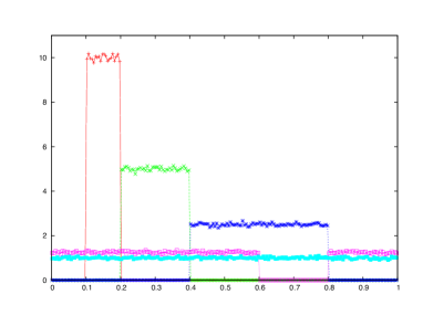
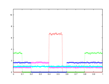
Figure 1: Probability density $\rho(x,t)$ for Bernoulli’s shift. The distribution is obtained generating at random 100000 points, uniformly distributed in the interval $[0.1:0.2]$ (a) and $[0.4:0.55]$ (b), and then iterating the dynamics of each point for 14 time steps. The red curves correspond to the initial distribution, the green, the blue, and the magenta curves correspond to one, two and three time steps, respectively. As it is evident, at each time step the dynamics initially doubles the width of interval over which the points are distributed, until $\rho(x,t)\approx\rho^{inv}(x)=1$. The light blue curves are obtained after 14 iterations: The probability density $\rho(x,t)$ for $t>12$ is close to the invariant distribution $\rho^{inv}(x)$ independently of the initial $\rho(x,0)$.

We saw how chaotic systems and, more precisely, those which are ergodic, naturally lead to probabilistic descriptions, even in the presence of deterministic dynamics. In particular, ergodic theory justifies the frequentist interpretation of probability, according to which the probability of a given event is defined by its relative frequency. Therefore, assuming ergodicity, it is possible to obtain an empirical notion of probability which is an objective property of the trajectory (von Plato 1994). There is no universal agreement on this issue; for instance, Popper (2002) believed that probabilistic concepts are extraneous to a deterministic description of the world, while Einstein held the opposite view, as expressed in his letter to Popper:

I do not believe that you are right in your thesis that it is impossible to derive statistical conclusions from a deterministic theory. Only think of classical statistical mechanics (gas theory, or the theory of Brownian movement).

6 A brief digression on models in physics

At this point of the discussion, we wish to recall that our description of physical phenomena is necessarely based upon models, that entail a schematization of a specified portion of the physical world. Take for instance the pendulum described by Eq. (1). The mathematical object introduced thereby relates to a physical pendulum under some specific assumptions. For instance, the string of length $L$, that connects the swinging body to a suspension point, is assumed to be inextensible, whereas any physical string is (to some extent) extensible. The model also assumes that gravity is spatially uniform and does not change with time, i.e., it can be described by a constant $g$. Eq. (1) will therefore reasonably describe a physical pendulum only inasmuch as the variations of $L$ and/or $g$ are sufficiently small, so as to add only tiny corrections. Even more important, there is not in the physical world such an object as an isolated pendulum, whereas Eq. (1) totally ignores the physical world around the pendulum (the only ingredients being gravity, the string, and the suspension point). Galileo Galilei was well aware of this subtlety when comparing the prediction of our mathematical models with the physical phenomena they aim to describe and called accidents (on this topic, see, e.g., Koertge, 1977) all external influences apt to modify, often in an apparently unpredictable way, the behaviour of a (supposedly isolated) portion of the physical world. In the case of the Eq. (1), we are, e.g., neglecting the fact that a real pendulum swings in a viscous medium (the air), and also experiences some friction at the suspension point. These effects gradually alter the motion of the pendulum, which is no longer periodic and eventually stops. Eq. (1) also neglects the fact that the Earth is not an inertial reference frame: it rotates around its axis and around the Sun. The first effect is far more important and gives rise to the gradual but sizable variation of the plane of oscillation (Foucault’s pendulum). There are several external influences that may alter the motion of a pendulum. Some of them may be accounted for, at least to some extent, by simple modifications of Eq. (1). Other are rather complicated and are not easily accountable. Thus, Eq. (1) describes a pendulum only as far and as long as external influences do not alter significantly its motion. Said in other words, it describes a pendulum under controlled conditions.

7 The old dilemma determinism/stochasticity

The above premise underlines the crucial importance of the concept of state of the system, i.e., in mathematical terms, the variables which describe the phenomenon under investigation. The relevance of such an aspect is often underestimated; only in few situations, e.g., in mechanical systems, it is easy to identify the variables which describe the phenomenon. On the contrary, in a generic case, there are serious difficulties; we can say that often the main effort in building a theory of nontrivial phenomena concerns the identification of the appropriate variables. Such a difficulty is well known in statistical physics; it has been stressed, e.g., by Onsager and Machlup (1953) in their seminal work on fluctuations and irreversible processes, with the caveat:

how do you know you have taken enough variables, for it to be Markovian?

In a similar way, Ma (1985) notes that:

the hidden worry of thermodynamics is: we do not know how many coordinates or forces are necessary to completely specify an equilibrium state.

Unfortunately, we have no definite method for selecting the proper variables.

Takens (1981) showed that from the study of a time series $\{u_{1},u_{2},...,u_{m}\}$, where $u$ is an observable sampled at the discrete times $t_{j}=j\Delta t$ and $u_{j}=u(t_{j})$, it is possible (if we know that the system is deterministic and is described by a finite dimensional vector) to determine the proper variable ${\bf X}$. Unfortunately the method has rather severe limitations:
a) It works only if we know a priori that the system is deterministic;
b) The protocol fails if the dimension of the attractor is large enough (say more than $5$ or $6$).
Therefore the method cannot be used, apart for special cases (with a small dimension), to build up a model from the data.

We already considered arguments, e.g., by van Kampen, which deny that determinism may be decided on the basis of observations. This conclusion is also reached from detailed analyses of sequences of data produced by the time evolutions of interest. In few words: the distinction between deterministic chaotic systems and genuine stochastic processes is possible if one is able to reach arbitrary precision on the state of the system.

Computing the so-called $\epsilon$-entropy $h(\epsilon)$, at different resolution scales $\epsilon$, at least in principle, one can distinguish potentially underlying deterministic dynamics from stochastic ones.

From a mathematical point of view the scenario is quite simple: for a deterministic chaotic system as $\epsilon\to 0$ one has $h(\epsilon)\to h_{KS}<\infty$, while for stochastic processes $h(\epsilon)\to\infty$. On the other hand an arbitrary solution is not possible, therefore the analysis of temporal series can only be used, at best, to pragmatically classify the stochastic or chaotic character of the observed signal, within certain scales (Cencini, et al., 2009; Franceschelli, 2012). At first, this could be disturbing: not even the most sophisticated time-series analysis that we could perform reveals the “true nature” of the system under investigation, the reason simply being the unavoidable finiteness of the resolution we can achieve.

On the other hand, one may be satisfied with a non-metaphysical point of view, in which the true nature of the object under investigation is not at stake. The advantage is that one may choose whatever model is more appropriate or convenient to describe the phenomenon of interest, especially considering the fact that, in practice, one observes (and wishes to account for) only a limited set of coarse-grained properties.
In light of our arguments, it seems fair to claim that the vexed question of whether the laws of physics are deterministic or probabilistic has, and will have, no definitive answer. On the sole basis of empirical observations, it does not appear possible to decide between these two contrasting arguments:
(i) Laws governing the Universe are inherently random, and the determinism that is believed to be observed is in fact a result of the probabilistic nature implied by the large number of degrees of freedom;
(ii) The fundamental laws are deterministic, and seemingly random phenomena appear so due to deterministic chaos.

Basically these two positions can be viewed as a reformulation of the endless debate on quantum mechanics: thesis (i) expresses the inherent indeterminacy claimed by the Copenhagen school, whereas thesis (ii) illustrates the hidden determinism advocated by Einstein (Pais 2005).



References

* Atmanspacher, H. “Determinism is ontic, determinability is epistemic”. In: Atmanspacher, H., Bishop, R. (eds.) Between Chance and Choice. (Imprint Academic, Thorverton, 2002)
* Boyd, R. “Determinism, laws and predictability in principle” Phylosophy of Science 39, 43 (1972)
* Campbell, L., Garnett, W. The Life of James Clerk Maxwell (MacMillan and Co., London, 1882)
* Cencini, M., Cecconi, F., Vulpiani, A. Chaos: From Simple Models to Complex Systems (World Scientific, Singapore, 2009)
* Chibbaro, S., Rondoni, L., Vulpiani, A. Reductionism, Emergence and Levels of Reality (Springer-Verlag, Berlin, 2014)
* Dyson, F. “Birds and frogs” Not. AMS 56, 212 (2009)
* Franceschelli, S. “Some remarks on the compatibility between determinism and unpredictability” Progr. in Bioph. and Mol. Bio. 110, 61 (2012)
* Galilei, G. “Dialogues concerning two new sciences” (MacMillan, New York, 1914)
* van Kampen, N. G. “Determinism and predictability” Synthese 89, 273 (1991)
* Koertge, N. “Galileo and the problem of accidents”, Journal of the History of Ideas 38, 389 (1977).
* Lorenz, E. N. “Deterministic nonperiodic flow” J. Atmos. Sci 20, 130 (1963)
* Ma, S. K. Statistical Mechanics (World Scientific, Singapore, 1985)
* Onsager, L., Machlup, S. “Fluctuations and irreversible processes” Phys. Rev. 91, 1505 (1953)
* Pais, A. Subtle is the Lord: The Science and the Life of Albert Einstein (Oxford University Press, 2005)
* Poincaré, H. Les méthodes nouvelles de la mécanique céleste (Gauthier-Villars, Paris, 1982)
* Popper, K.R. The Open Universe: An Argument for Indeterminism. From the Postscript to the Logic of Scientific Discovery (Routledge, London, 1992)
* Popper, K. R. The Logic of Scientific Discovery (Routledge, London, 2002)
* Prigogine, I., Stengers, I. Les Lois du Chaos (Flammarion, Paris 1994)
* Primas, H. “Hidden determinism, probability, and times arrow” In: Bishop, R., Atmanspacher, H. (eds.) Between Chance and Choice, p. 89 (Imprint Academic, Exeter 2002)
* Shannon, C. E. “A note on the concept of entropy” Bell System Tech. J. 27, 379 (1948)
* Stone, M. A. ”Chaos, prediction and Laplacean determinism” Am. Phylos. Quarterly 26, 123 (1989)
* Takens, F. ”Detecting strange attractors in turbulence”, In: D. Rand, L.-S. Young (eds.), Dynamical Systems and Turbulence, Lecture Notes in Mathematics 898 (1981), Springer-Verlag.
* von Plato, J. Creating Modern Probability (Cambridge University Press, 1994)
* Vauclair, S. Elémentes de Physique Statistique (Interéditions, Paris 1993)