Random Fourier Features for Operator-Valued Kernels

Abstract

Devoted to multi-task learning and structured output learning, operator-valued kernels provide a flexible tool to build vector-valued functions in the context of Reproducing Kernel Hilbert Spaces. To scale up these methods, we extend the celebrated Random Fourier Feature methodology to get an approximation of operator-valued kernels. We propose a general principle for Operator-valued Random Fourier Feature construction relying on a generalization of Bochner’s theorem for translation-invariant operator-valued Mercer kernels. We prove the uniform convergence of the kernel approximation for bounded and unbounded operator random Fourier features using appropriate Bernstein matrix concentration inequality. An experimental proof-of-concept shows the quality of the approximation and the efficiency of the corresponding linear models on example datasets.

1 Introduction

Multi-task regression (Micchelli and Pontil, 2005), structured classification (Dinuzzo et al., 2011), vector field learning (Baldassarre et al., 2012) and vector autoregression (Sindhwani et al., 2013; Lim et al., 2015) are all learning problems that boil down to learning a vector while taking into account an appropriate output structure. A $p$-dimensional vector-valued model can account for couplings between the outputs for improved performance in comparison to $p$ independent scalar-valued models. In this paper we are interested in a general and flexible approach to efficiently implement and learn vector-valued functions, while allowing couplings between the outputs. To achieve this goal, we turn to shallow architectures, namely the product of a (nonlinear) feature matrix $\tilde{\Phi}(x)$ and a parameter vector $\theta$ such that $\tilde{f}(x)=\tilde{\Phi}(x)^{*}\theta$, and combine two appealing methodologies: Operator-Valued Kernel Regression and Random Fourier Features.

Operator-Valued Kernels (Micchelli and Pontil, 2005; Carmeli et al., 2010; Álvarez et al., 2012) extend the classic scalar-valued kernels to vector-valued functions. As in the scalar case, operator-valued kernels (OVKs) are used to build Reproducing Kernel Hilbert Spaces (RKHS) in which representer theorems apply as for ridge regression or other appropriate loss functional. In these cases, learning a model in the RKHS boils down to learning a function of the form $f(x)=\sum_{i=1}^{n}K(x,x_{i})\alpha_{i}$ where $x_{1},\ldots,x_{n}$ are the training input data and each $\alpha_{i},i=1,\ldots,n$ is a vector of the output space $\mathcal{Y}$ and each $K(x,x_{i})$, an operator on vectors of $\mathcal{Y}$. However, OVKs suffer from the same drawback as classic kernel machines: they scale poorly to very large datasets because they are very demanding in terms of memory and computation. Therefore, focusing on the case $\mathcal{Y}=\mathbb{R}^{p}$, we propose to approximate OVKs by extending a methodology called Random Fourier Features (RFFs) (Rahimi and Recht, 2007; Le et al., 2013; Yang et al., 2014; Sriperumbudur and Szabo, 2015; Bach, 2015; Sutherland and Schneider, 2015) so far developed to speed up scalar-valued kernel machines. The RFF approach linearizes a shift-invariant kernel model by generating explicitly an approximated feature map $\tilde{\phi}$. RFFs has been shown to be efficient on large datasets and further improved by efficient matrix computations of FastFood (Le et al., 2013), and is considered as one of the best large scale implementations of kernel methods, along with Nÿstrom approaches (Yang et al., 2012).

In this paper, we propose general Random Fourier Features for functions in vector-valued RKHS. Here are our contributions: (1) we define a general form of Operator Random Fourier Feature (ORFF) map for shift-invariant operator-valued kernels, (2) we construct explicit operator feature maps for a simple bounded kernel, the decomposable kernel, and more complex unbounded kernels curl-free and divergence-free kernels, (3) the corresponding kernel approximation is shown to uniformly converge towards the target kernel using appropriate Bernstein matrix concentration inequality, for both bounded and unbounded operator-valued kernels and (4) we illustrate the theoretical approach by a few numerical results.

The paper is organized as follows. In section 1.2, we recall Random Fourier Feature and Operator-valued kernels. In section 2, we use extension of Bochner’s theorem to propose a general principle of Operator Random Fourier Features and provide examples for decomposable, curl-free and divergence-free kernels. In section 3, we present a theorem of uniform convergence for bounded and unbounded ORFFs (proof is given in appendix B) and the conditions of its application. Section 4 shows an numerical illustration on learning linear ORFF-models. Section 5 concludes the paper. The main proofs of the paper are presented in Appendix.

1.1 Notations

The euclidean inner product in $\mathbb{R}^{d}$ is denoted $\langle\cdot,\cdot\rangle$ and the euclidean norm is denoted $\left\lVert\cdot\right\rVert$. The unit pure imaginary number $\sqrt{-1}$ is denoted $i$. $\mathcal{B}(\mathbb{R}^{d})$ is the Borel $\sigma$-algebra on $\mathbb{R}^{d}$. For a function $f:\mathbb{R}^{d}\rightarrow\mathbb{R}$, if $dx$ is the Lebesgue measure on $\mathbb{R}^{d}$, we denote $\mathcal{F}\left[f\right]$ its Fourier transform defined by:

$$\forall x\in\mathbb{R}^{d},\mathcal{F}\left[f\right](x)=\int_{\mathbb{R}^{d}}e^{-i\langle\omega,x\rangle}f(\omega)d\omega.$$

The inverse Fourier transform of a function $g$ is defined as

$$\mathcal{F}^{-1}\left[g\right](\omega)=\int_{\mathbb{R}^{d}}e^{i\langle x,\omega\rangle}f(\omega)dx.$$

It is common to define the Fourier transform of a (positive) measure $\mu$ by

$$\mathcal{F}\left[\mu\right](x)=\int_{\mathbb{R}^{d}}e^{-i\langle\omega,x\rangle}d\mu(\omega).$$

If $\mathcal{X}$ and $\mathcal{Y}$ are two vector spaces, we denote by $\mathcal{F}(\mathcal{X};\mathcal{Y})$ the vector space of functions $f:\mathcal{X}\to\mathcal{Y}$ and $\mathcal{C}(\mathcal{X};\mathcal{Y})\subset\mathcal{F}(\mathcal{X};\mathcal{Y})$ the subspace of continuous functions. If $\mathcal{H}$ is an Hilbert space we denote its scalar product by $\langle.,.\rangle_{\mathcal{H}}$ and its norm by $\left\lVert.\right\rVert_{\mathcal{H}}$. We set $\mathcal{L}(\mathcal{H})=\mathcal{L}(\mathcal{H};\mathcal{H})$ to be the space of linear operators from $\mathcal{H}$ to itself. If $W\in\mathcal{L}(\mathcal{H})$, $\text{Ker}\;W$ denotes the nullspace, $\text{Im}\;W$ the image and $W^{*}\in\mathcal{L}(\mathcal{H})$ the adjoint operator (transpose in the real case).

1.2 Background

Random Fourier Features:

we first consider scalar-valued functions. Denote $k:\mathbb{R}^{d}\times\mathbb{R}^{d}\rightarrow\mathbb{R}$ a positive definite kernel on $\mathbb{R}^{d}$. A kernel $k$ is said to be shift-invariant for the addition if for any $a\in\mathbb{R}^{d}$, $\forall(x,x^{\prime})\in\mathbb{R}^{d}\times\mathbb{R}^{d},k(x-a,z-a)=k(x,z)$. Then, we define $k_{0}:\mathbb{R}^{d}\rightarrow\mathbb{R}$ the function such that $k(x,z)=k_{0}(x-z)$. $k_{0}$ is called the signature of kernel $k$. Bochner theorem is the theoretical result that leads to the Random Fourier Features.

Theorem 1.1 (Bochner’s theorem).

Every positive definite complex valued function is the Fourier transform of a non-negative measure. This implies that any positive definite, continuous and shift-invariant kernel $k$ is the Fourier transform of a non-negative measure $\mu$:

$$k(x,z)=k_{0}(x-z)=\int_{\mathbb{R}^{d}}e^{-i\langle\omega,x-z\rangle}d\mu(\omega).$$ (1)

Without loss of generality for the Random Fourier methodology, we assume that $\mu$ is a probability measure, i.e. $\int_{\mathbb{R}^{d}}d\mu(\omega)=1$. Then we can write eq. 1 as an expectation over $\mu$: $k_{0}(x-z)={\mathbb{E}}_{\mu}\left[e^{-i\langle\omega,x-z\rangle}\right]$. Both $k$ and $\mu$ are real-valued, and the imaginary part is null if and only if $\mu(\omega)=\mu(-\omega)$. We thus only write the real part:

$$k(x,z) ={\mathbb{E}}_{\mu}[\cos\langle\omega,x-z\rangle]$$

$$={\mathbb{E}}_{\mu}\left[\cos\langle\omega,z\rangle\cos\langle\omega,x\rangle+\sin\langle\omega,z\rangle\sin\langle\omega,x\rangle\right].$$

Let $\operatorname*{\bigoplus}_{j=1}^{D}x_{j}$ denote the $Dm$-length column vector obtained by stacking vectors $x_{j}\in\mathbb{R}^{m}$. The feature map $\tilde{\phi}:\mathbb{R}^{d}\rightarrow\mathbb{R}^{2D}$ defined as

$$\tilde{\phi}(x)=\frac{1}{\sqrt{D}}\operatorname*{\bigoplus}_{j=1}^{D}\begin{pmatrix}\cos{\langle x,\omega_{j}\rangle}\\ \sin{\langle x,\omega_{j}\rangle}\end{pmatrix},\enskip\omega_{j}\sim\mu$$ (2)

is called a Random Fourier Feature map. Each $\omega_{j},j=1,\ldots,D$ is independently sampled from the inverse Fourier transform $\mu$ of $k_{0}$. This Random Fourier Feature map provides the following Monte-Carlo estimator of the kernel:

$$\tilde{K}(x,z)=\tilde{\phi}(x)^{*}\tilde{\phi}(z),$$ (3)

that is proven to uniformly converge towards the true kernel described in eq. 1. The dimension $D$ governs the precision of this approximation whose uniform convergence towards the target kernel can be found in Rahimi and Recht (2007) and in more recent papers with some refinements Sutherland and Schneider (2015); Sriperumbudur and Szabo (2015). Finally, it is important to notice that Random Fourier Feature approach only requires two steps before learning: (1) define the inverse Fourier transform of the given shift-invariant kernel, (2) compute the randomized feature map using the spectral distribution $\mu$. For the Gaussian kernel $k(x-z)=exp(-\gamma\left\lVert x-z\right\rVert^{2})$, the spectral distribution $\mu(\omega)$ is Gaussian Rahimi and Recht (2007).

Operator-valued kernels:

we now turn to vector-valued functions and consider vector-valued Reproducing Kernel Hilbert spaces (vv-RKHS) theory. The definitions are given for input space $\mathcal{X}\subset\mathbb{C}^{d}$ and output space $\mathcal{Y}\subset\mathbb{C}^{p}$. We will define operator-valued kernel as reproducing kernels following the presentation of Carmeli et al. (2010). Given $\mathcal{X}$ and $\mathcal{Y}$, a map $K:\mathcal{X}\times\mathcal{X}\to\mathcal{L}(\mathcal{Y})$ is called a $\mathcal{Y}$-reproducing kernel if

$$\sum_{i,j=1}^{N}\langle K(x_{i},x_{j})y_{j},y_{i}\rangle\geq 0,$$

for all $x_{1},\ldots,x_{N}$ in $\mathcal{X}$, all $y_{1},\ldots,y_{N}$ in $\mathcal{Y}$ and $N\geq 1$. Given $x\in\mathcal{X}$, $K_{x}:\mathcal{Y}\to\mathcal{F}(\mathcal{X};\mathcal{Y})$ denotes the linear operator whose action on a vector $y$ is the function $K_{x}y\in\mathcal{F}(\mathcal{X};\mathcal{Y})$ defined by $(K_{x}y)(z)=K(z,x)y,\enskip\forall z\in\mathcal{X}$.

Additionally, given a $\mathcal{Y}$-reproducing kernel $K$, there is a unique Hilbert space $\mathcal{H}_{K}\subset\mathcal{F}(\mathcal{X};\mathcal{Y})$ satisfying $K_{x}\in\mathcal{L}(\mathcal{Y};\mathcal{H}_{K}),\enskip\forall x\in\mathcal{X}$ and $f(x)=K^{*}_{x}f,\enskip\forall x\in\mathcal{X},\forall f\in\mathcal{H}_{K}$, where $K^{*}_{x}:\mathcal{H}_{K}\to\mathcal{Y}$ is the adjoint of $K_{x}$. The space $\mathcal{H}_{K}$ is called the (vector-valued) Reproducing Kernel Hilbert Space associated with $K$. The corresponding product and norm are denoted by $\langle.,.\rangle_{K}$ and $\left\lVert.\right\rVert_{K}$, respectively. As a consequence (Carmeli et al., 2010) we have:

$$K(x,z) =K^{*}_{x}K_{z}\enskip\forall x,z\in\mathcal{X}$$

$$\mathcal{H}_{K} =\operatorname{\overline{span}\;}\left\{K_{x}y\enskip\middle|\enskip\forall x\in\mathcal{X},\enskip\forall y\in\mathcal{Y}\right\}$$

Another way to describe functions of $\mathcal{H}_{K}$ consists in using a suitable feature map.

Proposition 1.1 (Carmeli et al. (2010)).

Let $\mathcal{H}$ be a Hilbert space and $\Phi:\mathcal{X}\to\mathcal{L}(\mathcal{Y};\mathcal{H})$, with $\Phi_{x}\triangleq\Phi(x)$. Then the operator $W:\mathcal{H}\to\mathcal{F}(\mathcal{X};\mathcal{Y})$ defined by $(Wg)(x)=\Phi_{x}^{*}g,\enskip\forall g\in\mathcal{H},\forall x\in\mathcal{X}$ is a partial isometry from $\mathcal{H}$ onto the reproducing kernel Hilbert space $\mathcal{H}_{K}$ with reproducing kernel

$$K(x,z)=\Phi^{*}_{x}\Phi_{z},\enskip\forall x,z\in\mathcal{X}.$$

$W^{*}W$ is the orthogonal projection onto

$$\text{Ker}\;W^{\bot}=\operatorname{\overline{span}\;}\left\{\Phi_{x}y\enskip\middle|\enskip\forall x\in\mathcal{X},\enskip\forall y\in\mathcal{Y}\right\}.$$

Then $\left\lVert f\right\rVert_{K}=\inf\left\{\left\lVert g\right\rVert_{\mathcal{H}}\enskip\middle|\enskip\forall g\in\mathcal{H},\enskip Wg=f\right\}$.

We call $\Phi$ a feature map, $W$ a feature operator and $\mathcal{H}$ a feature space.

In this paper, we are interested on finding feature maps of this form for shift-invariant $\mathbb{R}^{p}$-Mercer kernels using the following definitions. A reproducing kernel $K$ on $\mathbb{R}^{d}$ is a $\mathbb{R}^{p}$-Mercer provided that $\mathcal{H}_{K}$ is a subspace of $\mathcal{C}(\mathbb{R}^{d};\mathbb{R}^{p})$. It is said to be a shift-invariant kernel or a translation-invariant kernel for the addition if $K(x+a,z+a)=K(x,z),\forall(x,z,a)\in\mathcal{X}^{3}$. It is characterized by a function $K_{0}:\mathcal{X}\to\mathcal{L}(\mathcal{Y})$ of completely positive type such that $K(x,z)=K_{0}(\delta)$, with $\delta=x-z$.

2 Operator-valued Random Fourier Features

2.1 Spectral representation of shift-invariant vector-valued Mercer kernels

The goal of this work is to build approximated matrix-valued feature map for shift-invariant $\mathbb{R}^{p}$-Mercer kernels, denoted with $K$, such that any function $f\in\mathcal{H}_{K}$ can be approximated by a function $\tilde{f}$ defined by:

$$\tilde{f}(x)=\tilde{\Phi}(x)^{*}\theta$$

where $\tilde{\Phi}(x)$ is a matrix of size $(m\times p)$ and $\theta$ is an $m$-dimensional vector. We propose a randomized approximation of such a feature map using a generalization of the Bochner theorem for operator-valued functions. For this purpose, we build upon the work of Carmeli et al. (2010) that introduced the Fourier representation of shift-invariant Operator-Valued Mercer Kernels on locally compact Abelian groups $\mathcal{X}$ using the general framework of Pontryagin duality (see for instance Folland (1994)). In a few words, Pontryagin duality deals with functions on locally compact Abelian groups, and allows to define their Fourier transform in a very general way. For sake of simplicity, we instantiate the general results of Carmeli et al. (2010); Zhang et al. (2012) for our case of interest of $\mathcal{X}=\mathbb{R}^{d}$ and $\mathcal{Y}=\mathbb{R}^{p}$. The following proposition extends Bochner’s theorem to any shift-invariant $\mathbb{R}^{p}$-Mercer kernel.

Proposition 2.1 (Operator-valued Bochner’s theorem).

A continuous function $K$ from $\mathbb{R}^{d}\times\mathbb{R}^{d}$ to $\mathcal{L}(\mathbb{R}^{p})$ is a shift-invariant reproducing kernel if and only if $\forall x,z\in\mathbb{R}^{d}$, it is the Fourier transform of a positive operator-valued measure $\mathcal{M}:\mathcal{B}(\mathbb{R}^{d})\to\mathcal{L}_{+}(\mathbb{R}^{p})$:

$$K(x,z)=\int_{\mathbb{R}^{d}}e^{-i\langle x-z,\omega\rangle}d\mathcal{M}(\omega),$$

where $\mathcal{M}$ belongs to the set of all the $\mathcal{L}_{+}(\mathbb{R}^{p})$-valued measures of bounded variation on the $\sigma$-algebra of Borel subsets of $\mathbb{R}^{d}$.

However it is much more convenient to use a more explicit result that involves real-valued (positive) measures. The following proposition instantiates Prop. 13 in Carmeli et al. (2010) to matrix-valued operators.

Proposition 2.2 (Carmeli et al. (2010)).

Let $\mu$ be a positive measure on $\mathbb{R}^{d}$ and $A:\mathbb{R}^{d}\to\mathcal{L}(\mathbb{R}^{p})$ such that $\langle A(.)y,y^{\prime}\rangle\in L^{1}(\mathbb{R}^{d},d\mu)$ for all $y,y^{\prime}\in\mathbb{R}^{p}$ and $A(\omega)\geq 0$ for $\mu$-almost all $\omega$. Then, for all $\delta\in\mathbb{R}^{d}$, $\forall\ell,m\in{\left\{1,\ldots,p\right\}}$,

$$K_{0}(\delta)_{\ell m}=\int_{\mathbb{R}^{d}}e^{-i\langle\delta,\omega\rangle}A(\omega)_{\ell m}d\mu(\omega)$$ (4)

is the kernel signature of a shift-invariant $\mathbb{R}^{p}$-Mercer kernel $K$ such that $K(x,z)=K_{0}(x-z)$. In other terms, each real-valued function $K_{0}(\cdot)_{\ell m}$ is the Fourier transform of $A(\cdot)_{\ell m}p_{\mu}(\cdot)$ where $p_{\mu}(\omega)=\frac{d\mu}{d\omega}$ is the Radon-Nikodym derivative of the measure $\mu$, which is also called the density of the measure $\mu$. Any shift-invariant kernel is of the above form for some pair $(A(\omega),\mu(\omega))$.

This theorem is proved in Carmeli et al. (2010). When $p=1$ one can always assume $A$ is reduced to the scalar $1$, $\mu$ is still a bounded positive measure and we retrieve the Bochner theorem applied to the scalar case (theorem 1.1). Now we introduce the following proposition that directly is a direct consequence of proposition 2.2.

Proposition 2.3 (Feature map).

Given the conditions of proposition 2.2, we define $B(\omega)$ such that $A(\omega)=B(\omega)B(\omega)^{*}$. Then the function $\Phi:\mathbb{R}^{p}\rightarrow L^{2}(\mathbb{R}^{d},\mu;\mathbb{R}^{p})$ defined for all $x\in\mathbb{R}^{p}$ by

$$\forall y\in\mathbb{R}^{p},\enskip\left(\Phi_{x}y\right)(\omega)=e^{i\langle x,\omega\rangle}B(\omega)^{*}y$$ (5)

is a feature map of the shift-invariant kernel $K$, i.e. it satisfies for all $x,z$ in $\mathbb{R}^{d}$, $\Phi_{x}^{*}\Phi_{z}=K(x,z)$.

Thus, to define an approximation of a given operator-valued kernel, we need an inversion theorem that provides an explicit construction of the pair $A(\omega),\mu(\omega)$ from the kernel signature. Proposition 14 in Carmeli et al. (2010), instantiated to $\mathbb{R}^{p}$-Mercer kernel gives the solution.

Proposition 2.4 (Carmeli et al. (2010)).

Let $K$ be a shift-invariant $\mathbb{R}^{p}$-Mercer kernel. Suppose that $\forall z\in\mathbb{R}^{d},\forall y,y^{\prime}\in\mathbb{R}^{p}$, $\langle K_{0}(.)y,y^{\prime}\rangle\in L^{1}(\mathbb{R}^{d},dx)$ where $dx$ denotes the Lebesgue measure. Define $C$ such that $\forall\omega\in\mathbb{R}^{d},\forall\ell,m\in{\left\{1,\ldots,p\right\}}$,

$$C(\omega)_{\ell m}=\int_{\mathbb{R}^{d}}e^{i\langle\delta,\omega\rangle}K_{0}(\delta)_{\ell m}d\delta.$$ (6)

Then

1. $C(\omega)$ is an non-negative matrix for all $\omega\in\mathbb{R}^{d}$,

2. $\langle C(.)y,y^{\prime}\rangle\in L^{1}(\mathbb{R}^{d},d\omega)$ for all $y,y^{\prime}\in\mathbb{R}^{p}$,

3. for all $\delta\in\mathbb{R}^{d}$,$\forall\ell,m\in{\left\{1,\ldots,p\right\}}$,

   $$K_{0}(\delta)_{\ell m}=\int_{\mathbb{R}^{d}}e^{-i\langle\delta,\omega\rangle}C(\omega)_{\ell m}d\omega.$$

From eq. 4 and eq. 6, we can write the following equality concerning the matrix-valued kernel signature $K_{0}$, coefficient by coefficient: $\forall\delta\in\mathbb{R}^{d},\forall i,j\in{\left\{1,\ldots,p\right\}},$

$$\int_{\mathbb{R}^{d}}e^{-i\langle\delta,\omega\rangle}C(\omega)_{ij}d\omega=\int_{\mathbb{R}^{d}}e^{-i\langle\delta,\omega\rangle}A(\omega)_{ij}d\mu(\omega).$$

We then conclude that the following equality holds almost everywhere for $\omega\in\mathbb{R}^{d}$: $C(\omega)_{ij}=A(\omega)_{ij}p_{\mu}(\omega)$ where $p_{\mu}(\omega)=\frac{d\mu}{d\omega}$. Without loss of generality we assume that $\int_{\mathbb{R}^{d}}d\mu(\omega)=1$ and thus, $\mu$ is a probability distribution. Note that this is always possible through an appropriate normalization of the kernel. Then $p_{\mu}$ is the density of $\mu$. The proposition 2.2 thus results in an expectation:

$$K_{0}(x-z)={\mathbb{E}}_{\mu}[e^{-i\langle x-z,\omega\rangle}A(\omega)]$$ (7)

2.2 Construction of Operator Random Fourier Feature

Given a $\mathbb{R}^{p}$-Mercer shift-invariant kernel $K$ on $\mathbb{R}^{d}$, we build an Operator-Valued Random Fourier Feature (ORFF) map in three steps:

1. compute $C:\mathbb{R}^{d}\rightarrow\mathcal{L}(\mathbb{R}^{p})$ from eq. 6 by using the inverse Fourier transform (in the sense of proposition 2.4) of $K_{0}$, the signature of $K$;

2. find $A(\omega)$, $p_{\mu}(\omega)$ and compute $B(\omega)$ such that $A(\omega)=B(\omega)B(\omega)^{*}$;

3. build an randomized feature map via Monte-Carlo sampling from the probability measure $\mu$ and the application $B$.

2.3 Monte-Carlo approximation

Let $\operatorname{\bigoplus}_{j=1}^{D}X_{j}$ denote the block matrix of size $rD\times s$ obtained by stacking $D$ matrices $X_{1},\ldots,X_{D}$ of size $r\times s$. Assuming steps 1 and 2 have been performed, for all $j=1,\ldots,n$, we find a decomposition $A(\omega_{j})=B(\omega_{j})B(\omega_{j})^{*}$ either by exhibiting a general analytical closed-form or using a numerical decomposition. Denote $p\times p^{\prime}$ the dimension of the matrix $B(\omega)$. We then propose a randomized matrix-valued feature map: $\forall x\in\mathbb{R}^{d}$,

$$\tilde{\Phi}(x) =\frac{1}{\sqrt{D}}\operatorname*{\bigoplus}_{j=1}^{D}\Phi_{x}(\omega_{j}),\enskip\omega_{j}\sim\mu$$ (8)

$$=\frac{1}{\sqrt{D}}\operatorname*{\bigoplus}_{j=1}^{D}e^{-i\langle x,\omega_{j}\rangle}B(\omega_{j})^{*},\enskip\omega_{j}\sim\mu.$$

The corresponding approximation for the kernel is then: $\forall x,z\in\mathbb{R}^{d}$

$$\tilde{K}(x,z) =\tilde{\Phi}(x)^{*}\tilde{\Phi}(z)$$

$$=\frac{1}{D}\sum\nolimits_{j=1}^{D}e^{-i\langle x,\omega_{j}\rangle}B(\omega_{j})e^{i\langle z,\omega_{j}\rangle}B(\omega_{j})^{*}$$

$$=\frac{1}{D}\sum\nolimits_{j=1}^{D}e^{-i\langle x-z,\omega_{j}\rangle}A(\omega_{j}).$$

The Monte-Carlo estimator $\tilde{\Phi}(x)^{*}\tilde{\Phi}(z)$ converges in probability to $K(x,z)$ when $D$ tends to infinity. Namely,

$$\tilde{K}(x,z)=\tilde{\Phi}(x)^{*}\tilde{\Phi}(z)\xrightarrow[D\to\infty]{p.}{\mathbb{E}}_{\mu}\left[e^{-i\langle x-z,\omega\rangle}A(\omega)\right]=K(x,z)$$

As for the scalar-valued kernel, a real-valued matrix-valued function has a real matrix-valued Fourier transform if $A(\omega)$ is even with respect to $\omega$. Taking this point into account, we define the feature map of a real matrix-valued kernel as

$$\tilde{\Phi}(x)=\frac{1}{\sqrt{D}}\operatorname*{\bigoplus}_{j=1}^{D}\begin{pmatrix}\cos{\langle x,\omega_{j}\rangle}B(\omega_{j})^{*}\\ \sin{\langle x,\omega_{j}\rangle}B(\omega_{j})^{*}\end{pmatrix},\enskip\omega_{j}\sim\mu.$$

The kernel approximation becomes

$$\tilde{\Phi}(x)^{*}\tilde{\Phi}(z) =\frac{1}{D}\sum_{j=1}^{D}\begin{subarray}{c}\cos{\langle x,\omega_{j}\rangle}\cos{\langle z,\omega_{j}\rangle}A(\omega_{j})\\ \sin{\langle x,\omega_{j}\rangle}\sin{\langle z,\omega_{j}\rangle}A(\omega_{j})\end{subarray}+$$

$$=\frac{1}{D}\sum_{j=1}^{D}\cos{\langle x-z,\omega_{j}\rangle}A(\omega_{j}).$$

In the following, we give an explicit construction of ORFFs for three well-known $\mathbb{R}^{p}$-Mercer and shift-invariant kernels: the decomposable kernel introduced in Micchelli and Pontil (2005) for multi-task regression and the curl-free and the divergence-free kernels studied in Macedo and Castro (2008); Baldassarre et al. (2012) for vector field learning. All these kernels are defined using a scalar-valued shift-invariant Mercer kernel $k:\mathbb{R}^{d}\times\mathbb{R}^{d}\to\mathbb{R}$ whose signature is denoted $k_{0}$. A usual choice is to choose $k$ as a Gaussian kernel with $k_{0}(\delta)=\exp\left(-\frac{\left\lVert\delta\right\rVert^{2}}{2\sigma^{2}}\right)$, which gives $\mu=\mathcal{N}(0,\sigma^{-2}I)$ (Huang et al., 2013) as its inverse Fourier transform.

Definition 2.1 (Decomposable kernel).

Let A be a $(p\times p)$ positive semi-definite matrix. $K$ defined as $\forall(x,z)\in\mathbb{R}^{d}\times\mathbb{R}^{d},K(x,z)=k(x,z)A$ is a $\mathbb{R}^{p}$-Mercer shift-invariant reproducing kernel.

Matrix $A$ encodes the relationships between the outputs coordinates. If a graph coding for the proximity between tasks is known, then it is shown in Evgeniou et al. (2005); Baldassarre et al. (2010) that $A$ can be chosen equal to the pseudo inverse $L^{\dagger}$ of the graph Laplacian, and then the $\ell_{2}$ norm in $\mathcal{H}_{K}$ is a graph-regularizing penalty for the outputs (tasks). When no prior knowledge is available, $A$ can be set to the empirical covariance of the output training data or learned with one of the algorithms proposed in the literature (Dinuzzo et al., 2011; Sindhwani et al., 2013; Lim et al., 2015). Another interesting property of the decomposable kernel is its universality. A reproducing kernel $K$ is said universal if the associated RKHS $\mathcal{H}_{K}$ is dense in the space $\mathcal{C}(\mathcal{X},\mathcal{Y})$.

Example 2.1 (ORFF for decomposable kernel).

$$C^{dec}(\omega)_{\ell m}=\int_{\mathcal{X}}e^{i\langle\delta,\omega\rangle}k_{0}(\delta)A_{\ell m}d\delta=A_{\ell m}\mathcal{F}^{-1}\left[k_{0}\right](\omega)\\$$

Hence, $A^{dec}(\omega)=A$ and $p_{\mu}^{dec}(\omega)=\mathcal{F}^{-1}\left[k_{0}\right](\omega)$.

ORFF for curl-free and div-free kernels:

Curl-free and divergence-free kernels provide an interesting application of operator-valued kernels (Macedo and Castro, 2008; Baldassarre et al., 2012; Micheli and Glaunes, 2013) to vector field learning, for which input and output spaces have the same dimensions ($d=p$). Applications cover shape deformation analysis (Micheli and Glaunes, 2013) and magnetic fields approximations (Wahlström et al., 2013). These kernels discussed in Fuselier (2006) allow encoding input-dependent similarities between vector-fields.

Definition 2.2 (Curl-free and Div-free kernel).

We have $d=p$. The divergence-free kernel is defined as

$$K^{div}(x,z)=K^{div}_{0}(\delta)=(\nabla\nabla^{*}-\Delta I)k_{0}(\delta)$$

and the curl-free kernel as

$$K^{curl}(x,z)=K_{0}^{curl}(\delta)=-\nabla\nabla^{*}k_{0}(\delta),$$

where $\nabla\nabla^{*}$ is the Hessian operator and $\Delta$ is the Laplacian operator.

Although taken separately these kernels are not universal, a convex combination of the curl-free and divergence-free kernels allows to learn any vector field that satisfies the Helmholtz decomposition theorem (Macedo and Castro, 2008; Baldassarre et al., 2012). For the divergence-free and curl-free kernel we use the differentiation properties of the Fourier transform.

Example 2.2 (ORFF for curl-free kernel:).

$\forall\ell,m\in{\left\{1,\ldots,p\right\}}$,

$$C^{curl}(\omega)_{\ell m} =-\mathcal{F}^{-1}\left[\frac{\partial}{\partial\delta_{\ell}}\frac{\partial}{\partial\delta_{m}}k_{0}\right](\omega)$$

$$=\omega_{\ell}\omega_{m}\mathcal{F}^{-1}\left[k_{0}\right](\omega)$$

Hence, $A^{curl}(\omega)=\omega\omega^{*}$ and $p_{\mu}^{curl}(\omega)=\mathcal{F}^{-1}\left[k_{0}\right](\omega)$. We can obtain directly: $B^{curl}(\omega)=\omega$.

For the divergence-free kernel we first compute the Fourier transform of the Laplacian of a scalar kernel using differentiation and linearity properties of the Fourier transform. We denote $\delta_{\{\ell=m\}}$ as the Kronecker delta which is $1$ if $\ell=m$ and zero otherwise.

Example 2.3 (ORFF for divergence-free kernel:).

$$C^{div}(\omega)_{\ell m} =\mathcal{F}^{-1}\left[\frac{\partial}{\partial\delta_{\ell}}\frac{\partial}{\partial\delta_{m}}k_{0}-\delta_{\{\ell=m\}}\Delta k_{0}\right]$$

$$=\mathcal{F}^{-1}\left[\frac{\partial}{\partial\delta_{\ell}}\frac{\partial}{\partial\delta_{m}}k_{0}\right]-\delta_{\{\ell=m\}}\mathcal{F}^{-1}\left[\Delta k_{0}\right]$$

$$=(\delta_{\{\ell=m\}}-\omega_{\ell}\omega_{m})\left\lVert\omega\right\rVert_{2}^{2}\mathcal{F}^{-1}\left[k_{0}\right],$$

since

$$\mathcal{F}^{-1}\left[\Delta k_{0}(\delta)\right]=\sum_{k=1}^{p}\mathcal{F}^{-1}\left[\frac{\partial}{\partial\delta_{k}}k_{0}\right]=-\left\lVert\omega\right\rVert_{2}^{2}\mathcal{F}^{-1}\left[k_{0}\right].$$

Hence $A^{div}(\omega)=I\left\lVert\omega\right\rVert_{2}^{2}-\omega\omega^{*}$ and $p_{\mu}^{div}(\omega)=\mathcal{F}^{-1}\left[k_{0}\right](\omega)$. Here, $B^{div}(\omega)$ has to be obtained by a numerical decomposition such as Cholesky or SVD.

Figure 1: Empirical Approximation Error versus number of random features $D$ induced by the ORFF approximation for different operator-valued kernels

3 Uniform error bound on ORFF approximation

We are now interested on measuring how close the approximation $\tilde{K}(x,z)=\tilde{\Phi}(x)^{*}\tilde{\Phi}(z)$ is close to the target kernel $K(x,z)$ for any $x,z$ in a compact set $\mathcal{C}$. If $A$ is a real matrix, we denote $\left\lVert A\right\rVert_{2}$ its spectral norm, defined as the square root of the largest eigenvalue of $A$. For $x$ and $z$ in some compact $\mathcal{C}\subset\mathbb{R}^{d}$, we consider: $F(x-z)=\tilde{K}(x,z)-K(x,z)$ and study how the uniform norm

$$\left\lVert F\right\rVert_{\infty}=\sup_{x,z\in\mathcal{C}}\left\lVert\tilde{K}(x,z)-K(x,z)\right\rVert_{2}$$ (9)

behaves according to $D$. Figure 1 empirically shows convergence of three different OVK approximations for $x,z$ from the compact $[-1,1]^{4}$ using an increasing number of sample points $D$. The log-log plot shows that all three kernels have the same convergence rate, up to a multiplicative factor.

In order to bound the error with high probability, we turn to concentration inequalities devoted to random matrices (Boucheron et al., ). In the case of the decomposable kernel, the answer to that question can be directly obtained as a consequence of the uniform convergence of RFFs in the scalar case obtained by Rahimi and Recht (2007) and other authors (Sutherland and Schneider, 2015; Sriperumbudur and Szabo, 2015) since in this case,

$$\left\lVert\tilde{K}(x,z)-K(x,z)\right\rVert_{2}=\left\lVert A\right\rVert_{2}\left\lVert\tilde{k}(x,z)-k(x,z)\right\rVert$$

This theorem and its proof are presented in corollary A.1.1.

More interestingly, we propose a new bound for Operator Random Fourier Feature approximation in the general case. It relies on three main ideas: (i) Matrix concentration inequality for random matrices has to be used instead of concentration inequality for (scalar) random variables, (ii) Instead of using Hoeffding inequality as in the scalar case (proof of Rahimi and Recht (2007)) but for matrix concentration (Mackey et al., 2014) we use a refined inequality such as the Bernstein matrix inequality (Ahlswede and Winter, ; Boucheron et al., ; Tropp, 2012), also used for the scalar case in (Sutherland and Schneider, 2015), (iii) we propose a general theorem valid for random matrices with bounded norms (case for decomposable kernel ORFF approximation) as well as with unbounded norms (curl and divergence-free kernels). For the latter, we notice that their norms behave as subexponential random variables (Koltchinskii et al., 2013). Before introducing the new theorem, we give the definition of the Orlicz norm and subexponential random variables.

Definition 3.1 (Orlicz norm).

We follow the definition given by Koltchinskii et al. (2013). Let $\psi:\mathbb{R}_{+}\to\mathbb{R}_{+}$ be a non-decreasing convex function with $\psi(0)=0$. For a random variable $X$ on a measured space $(\Omega,\mathcal{T}(\Omega),\mu)$,

$$\left\lVert X\right\rVert_{\psi}\triangleq\inf\left\{C>0\,\,\middle|\,\,{\mathbb{E}}[\psi\left(\left\lvert X\right\rvert/C\right)]\leq 1\right\}.$$

Here, the function $\psi$ is chosen as $\psi(u)=\psi_{\alpha}(u)$ where $\psi_{\alpha}(u)\triangleq e^{u^{\alpha}}-1$. When $\alpha=1$, a random variable with finite Orlicz norm is called a subexponential variable because its tails decrease at least exponentially fast.

Theorem 3.1.

Let $\mathcal{C}$ be a compact subset of $\mathbb{R}^{d}$ of diameter $l$. Let $K$ be a shift-invariant $\mathbb{R}^{p}$-Mercer kernel on $\mathbb{R}^{d}$, $K_{0}$ its signature and $p_{\mu}(\cdot)A(\cdot)$ the inverse Fourier transform of the kernel’s signature (in the sense of proposition 2.4) where $p_{\mu}$ is the density of a probability measure $\mu$ considering appropriate normalization. Let $D$ be a positive integer and $\omega_{1},\ldots,\omega_{D}$, i.i.d. random vectors drawn according to the probability law $\mu$. For $x,z\in\mathcal{C}$, we recall

$$\tilde{K}(x,z)=\sum_{j=1}^{D}\cos\langle x-z,\omega_{j}\rangle A(\omega_{j}).$$

We note for all $j\in{\left\{1,\ldots,D\right\}}$,

$$F_{j}(x-z)=\frac{1}{D}\left(\sum_{j=1}^{D}\cos\langle x-z,\omega_{j}\rangle A(\omega_{j})-K(x,z)\right)$$

and $F(x-z)=\tilde{K}(x,z)-K(x,z)$. $\left\lVert F\right\rVert_{\infty}$ denotes the infinite norm of $F(x-z)$ on the compact $\mathcal{C}$ as introduced in eq. 9. If one can define the following terms $(b_{D},m,\sigma_{p}^{2})\in\mathbb{R}^{3}_{+}$:

$$b_{D} =\sup_{x,z\in\mathcal{C}}D\left\lVert{\mathbb{E}}_{\mu}\left[\sum_{j=1}^{D}\left(F_{j}(x-z)\right)^{2}\right]\right\rVert_{2},$$

$$m =4\left(\left\lVert\left\lVert A(\omega)\right\rVert_{2}\right\rVert_{\psi_{1}}+\sup_{x,z\in\mathcal{C}}\left\lVert K(x,z)\right\rVert\right),\enskip\omega\sim\mu,$$

$$\sigma_{p}^{2} ={\mathbb{E}}_{\mu}\left[\left\lVert\omega\right\rVert_{2}^{2}\left\lVert A(\omega)\right\rVert_{2}^{2}\right].$$

Then for all $\epsilon$ in $\mathbb{R}_{+}$,

$${\mathbb{P}}\left\{\left\lVert F\right\rVert_{\infty}\geq\epsilon\right\}\leq C_{d}\left(\frac{\sigma_{p}l}{\epsilon}\right)^{\frac{2}{1+2/d}}\begin{cases}\exp\left(-\frac{\epsilon^{2}D}{8(d+2)\left(b_{D}+\frac{\epsilon\bar{u}_{D}}{6}\right)}\right)&\text{if}\enskip\bar{u}_{D}\leq\frac{2(e-1)b_{D}}{\epsilon}\\ \exp\left(-\frac{\epsilon D}{(d+2)(e-1)\bar{u}_{D}}\right)&\text{otherwise},\end{cases}$$

where $\bar{u}_{D}=2m\log\left(2^{\frac{3}{2}}\left(\frac{m}{b_{D}}\right)^{2}\right)$ and $C_{d}=p\left(\left(\frac{d}{2}\right)^{\frac{-d}{d+2}}+\left(\frac{d}{2}\right)^{\frac{2}{d+2}}\right)2^{\frac{6d+2}{d+2}}$.

We detail the proof of the theorem in appendix B. It follows the usual scheme derived in Rahimi and Recht (2007) and Sutherland and Schneider (2015) and involves Bernstein concentration inequality for unbounded symmetric matrices (theorem B.1).

3.1 Application to some operator-valued kernel

To apply theorem 3.1 to operator-valued kernels, we need to ensure that all the constants exist. In the following, we first show how to bound the constant term $b_{D}$. Then we exhibit the upper bounds for the three operator-valued kernels we took as examples. Eventually, we ensure that the random variable $\left\lVert A(\omega)\right\rVert$ has a finite Orlicz norm with $\psi=\psi_{1}$ in these three cases.

Bounding the term $b_{D}(\delta)$:

Proposition 3.1.

Define the matrix ${\mathbb{V}}_{\mu}[A(\omega)]$ as follows: for all $\ell,m\in{\left\{1,\ldots,p\right\}}$,

$${\mathbb{V}}_{\mu}[A(\omega)]_{\ell m}=\sum_{r=1}^{p}\text{Cov}_{\mu}[A(\omega)_{\ell r},A(\omega)_{rm}]$$

For a given $\delta=x-z$, define:

$$b_{D}(\delta)=D\left\lVert{\mathbb{E}}_{\mu}\left[\sum_{j=1}^{D}\left(F_{j}(\delta)\right)^{2}\right]\right\rVert_{2}.$$

Then we have:

$$b_{D}(\delta)\leq\frac{1}{2}\left\lVert(K_{0}(2\delta)+K_{0}(0)){\mathbb{E}}_{\mu}[A(\omega)]-2K_{0}(\delta)^{2}\right\rVert_{2}+\left\lVert{\mathbb{V}}_{\mu}[A(\omega)]\right\rVert_{2}.$$

The proof uses trigonometry properties and various properties of the moments and is given in appendix C. Now, we compute the upper bound given by proposition 3.1 for the three kernels we have taken as examples.

1. Decomposable kernel: notice that in the case of the Gaussian decomposable kernel, i.e. $A(\omega)=A$, $K_{0}(\delta)=Ak_{0}(\delta)$, $k_{0}(\delta)\geq 0$ and $k_{0}(\delta)=1$, then we have:

   $$b_{D}(\delta)\leq\frac{1}{2}(1+k_{0}(2\delta))\left\lVert A\right\rVert_{2}+k_{0}(\delta)^{2}$$

2. curl-free and div-free kernels: recall that in this case $p=d$. For the (Gaussian) curl-free kernel, $A(\omega)=\omega\omega^{*}$ where $\omega\in\mathbb{R}^{d}\sim\mathcal{N}(0,\sigma^{-2}I_{d})$ thus ${\mathbb{E}}_{\mu}[A(\omega)]=I_{d}/\sigma^{2}$ and ${\mathbb{V}}_{\mu}[A(\omega)]=(d+1)I_{d}/\sigma^{4}$ (see Petersen et al. (2008)). Hence,

   $$b_{D}(\delta)\leq\frac{1}{2}\left\lVert\frac{1}{\sigma^{2}}K_{0}(2\delta)-2K_{0}(\delta)^{2}\right\rVert_{2}+\frac{(d+1)}{\sigma^{4}}$$

   Eventually for the Gaussian divergence-free kernel, $A(\omega)=I\left\lVert\omega\right\rVert_{2}^{2}-\omega\omega^{*}$, thus ${\mathbb{E}}_{\mu}[A(\omega)]=I_{d}(d-1)/\sigma^{2}$ and ${\mathbb{V}}_{\mu}[A(\omega)]=d(4d-3)I_{d}/\sigma^{4}$ (see Petersen et al. (2008)). Hence,

   $$b_{D}(\delta)\leq\frac{1}{2}\left\lVert\frac{(d-1)}{\sigma^{2}}K_{0}(2\delta)-2K_{0}(\delta)^{2}\right\rVert_{2}+\frac{d(4d-3)}{\sigma^{4}}$$

An empirical illustration of these bounds is shown in fig. 6.

Computing the Orlicz norm:

For a random variable with strictly monotonic moment generating function (MGF), one can characterize its $\psi_{1}$ Orlicz norm by taking the functional inverse of the MGF evaluated at 2. In other words

$$\left\lVert X\right\rVert_{\psi_{1}}^{-1}=\text{MGF}(x)^{-1}_{X}(2).$$

For the Gaussian curl-free and divergence-free kernel

$$\left\lVert A^{div}(\omega)\right\rVert_{2}=\left\lVert A^{curl}(\omega)\right\rVert_{2}=\left\lVert\omega\right\rVert_{2}^{2}$$

where $\omega\sim\mathcal{N}(0,I_{d}/\sigma^{2})$, hence $\left\lVert A(\omega)\right\rVert_{2}\sim\Gamma(p/2,2/\sigma^{2})$. The MGF of this gamma distribution is $\text{MGF}(x)^{-1}(t)=(1-2t/\sigma^{2})^{-(p/2)}$. Eventually

$$\left\lVert\left\lVert A^{div}(\omega)\right\rVert_{2}\right\rVert_{\psi_{1}}^{-1}=\left\lVert\left\lVert A^{curl}(\omega)\right\rVert_{2}\right\rVert_{\psi_{1}}^{-1}=\frac{\sigma^{2}}{2}\left(1-4^{-\frac{1}{p}}\right).$$

4 Learning with ORFF

In practise, the previous bounds are however too large to find a safe value for $D$. In the following, numerical examples of ORFF-approximations are presented.

4.1 Penalized regression with ORFF

Once we have an approximated feature map, we can use it to provide a feature matrix of size $p^{\prime}D\times p$ with matrix $B(\omega)$ of size $p\times p^{\prime}$ such that $A(\omega)=B(\omega)B(\omega)^{*}$. A function $f\in\mathcal{H}_{K}$ is then approximated by a linear model

$$\tilde{f}(x)=\tilde{\Phi}(x)^{*}\theta,\enskip\text{where}\enskip\theta\in\mathbb{R}^{p^{\prime}D}.$$

Let $\mathcal{S}=\{(x_{i},y_{i})\in\mathbb{R}^{d}\times\mathbb{R}^{p},i=1,\ldots,N\}$ be a collection of i.i.d training samples. Given a local loss function $L:\mathcal{S}\to\mathbb{R}^{+}$ and a $\ell_{2}$ penalty, we minimize

$$\mathcal{L}(\theta)=\frac{1}{N}\sum_{i=1}^{N}L\left(\tilde{\Phi}(x_{i})^{*}\theta,y_{i}\right)+\lambda\left\lVert\theta\right\rVert_{2}^{2},$$ (10)

instead of minimizing $\mathcal{L}(f)=\frac{1}{N}\sum_{i=1}^{N}L(f(x_{i}),y_{i})+\lambda\left\lVert f\right\rVert^{2}_{\mathcal{H}_{K}}$. To find a minimizer of the optimization problem eq. 10 many optimization algorithms are available. For instance, in large-scale context, a stochastic gradient descent algorithm would be be suitable: we can adapt the algorithm to the kind of kernel/problematic. We investigate two optimization algorithms: a Stein equation solver appropriate for the decomposable kernel and a (stochastic) gradient descent for non-decomposable kernels (e.g. the curl-free and divergence-free kernels).

Closed form for the decomposable kernel:

for the real decomposable kernel $K_{0}(\delta)=k(\delta)A$ when $L(y,y^{\prime})=\left\lVert y-y^{\prime}\right\rVert_{2}^{2}$ (Kernel Ridge regression in $\mathcal{H}_{K}$), the learning problem described in eq. 10 can be re-written in terms of matrices to find the unique minimizer $\Theta_{*}$, where $\text{vec}(\Theta)=\theta$ such that $\theta$ is a $p^{\prime}D$ vector and $\Theta$ a $p^{\prime}\times D$ matrix. If $\tilde{\phi}$ is a feature map ($\tilde{\phi}(X)$ is a matrix of size $D\times N$) for the scalar kernel $k_{0}$, then

$$\tilde{\Phi}(x)^{*}\theta=(\tilde{\phi}(x)^{*}\otimes B)\theta=B\Theta\tilde{\phi}(x)$$

and

$$\theta_{*}=\operatorname*{arg\,min}_{\Theta\in\mathbb{R}^{p^{\prime}\times D}}\left\lVert B\Theta\tilde{\phi}(X)-Y\right\rVert_{F}^{2}+\lambda\left\lVert\Theta\right\rVert_{F}^{2}.$$ (11)

This is a convex optimization problem and a sufficient condition is:

$$\tilde{\phi}(X)\tilde{\phi}(X)^{*}\Theta_{*}B^{*}B-\tilde{\phi}(X)Y^{*}B+\lambda\Theta_{*}=0,$$

which is a Stein equation.

Gradient computation for the general case.

When it is not possible or desirable to use Stein’s equations solver one can apply a (stochastic) gradient descent algorithm. The gradient computation for and $\ell_{2}$-loss applied to ORFF model is briefly recalled in section D.1.

4.2 Numerical illustration

We present a few experiments to complete the theoretical contribution and illustrate the behavior of ORFF-regression. Other experimentalresults with noisy output data are shown in section D.2.

Figure 2: Computation time of ORFF and OVK on MNIST versus the number of datapoints $N$.

Figure 3: Prediction Error in percent on MNIST versus $D$, the number of Fourier features. In blue dashed line, ORFF and in red solid line OVK. For OVK and ORFF the number of datapoints $N=1000$.

Datasets:

the first dataset is the handwritten digits recognition dataset MNIST We select a training set of $12000$ images and a test set of $10000$ images. The inputs are images represented as a vector $x_{i}\in[0,255]^{784}$ and the targets are integers between $0$ and $9$. First we scaled the inputs such that they take values in $[-1,1]^{784}$. Then we binarize the targets such that each number is represented by a unique binary vector of length $10$. To predict classes, we use simplex coding method presented in Mroueh et al. (2012). The intuition behind simplex coding is to project the binarized labels of dimension $p$ onto the most separated vectors on the hypersphere of dimension $p-1$. For ORFF we can encode directly this projection in the $B$ matrix of the decomposable kernel $K_{0}(\delta)=BB^{*}k_{0}(\delta)$ where $k_{0}$ is a Gaussian kernel. For OVK we project the binarized targets on the simplex as a preprocessing step, before learning with the kernel $K_{0}(\delta)=I_{p}k_{0}(\delta)$, where $k_{0}$ is a also Gaussian kernel.

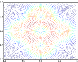
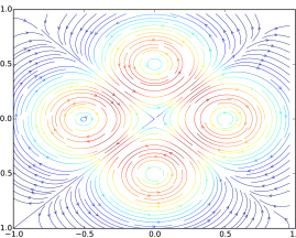
Curl-free	Divergence-free

Figure 7: Synthetic data used to train the curl-free and divergence free ORFF and OVK.

The second dataset corresponds to a 2D-vector field with structure. We generated a scalar field as a mixture of five Gaussians located at $[0,0]$, $[0,1]$, $[0,-1]$, with positive values and at $[-1,0]$, $[1,0]$ with negative values. The curl-free field has been generated by taking the gradient of the scalar-field, and the divergence-free field by taking the orthogonal of the curl-free field. These 2D-datasets are depicted in fig. 7.

Approximation:

We trained both an ORFF and an OVK model on the handwritten digits recognition dataset (MNIST) with a decomposable Gaussian kernel with signature $K_{0}(\delta)=\exp(-\left\lVert\delta\right\rVert/\sigma^{2})A$. To find a solution of the optimization problem described in eq. 11, we use off-the-shelf solver able to handle Stein’s equation. For both methods we choose $\sigma=20$ and use a $2$-fold cross validation on the training set to select the optimal $\lambda$. First, fig. 2 shows the running time comparison between OVK and ORFF models using $D=1000$ Fourier features against the number of datapoints $N$. The log-log plot shows ORFF scaling better than the OVK w.r.t the number of points. Second, fig. 3 shows the test prediction error versus the number of ORFFs $D$, when using $N=1000$ training points. As expected, the ORFF model converges toward the OVK model when the number of features increases.

Independent (RFF) prediction vs Structured prediction on vector fields:

we perform a similar experiment over a simulated dataset designed for learning a 2D-vector field with structure. Figure 4 reports the Mean Squared Error versus the number of ORFF $D$. For this experiment we use a Gaussian curl-free kernel and tune its $\sigma$ hyperparameter as well as the $\lambda$ on a grid. The curl-free ORFF outperforms classic RFFs by tending more quickly towards the noise level.

Figure 4: Mean squared (test) error on the synthetic data versus number of Fourier features $D$. The solid lines represent decomposable (blue) and curl (red) OVK methods while the dotted lines represent decomposable (blue) and curl (red) ORFF methods.

Figure 5 shows the computation time between curl-ORFF and curl-OVK indicating that the OVK solution does not scale to large datasets, while ORFF scales well with when the number of data increases. When $N>10^{4}$ exact OVK is not able to be trained in reasonable time ($>1000$ seconds).

Figure 5: Computation time of curl-ORFF and curl-OVK versus the number of datapoints on synthetic data. We fixed $D=1000$ Fourier features and study the computation time w.r.t the number of points.

5 Conclusion

We introduced a general and versatile framework for operator-valued kernel approximation with Operator Random Fourier Features. We showed the uniform convergence of these approximations by proving a matrix concentration inequality for bounded and unbounded ORFFs. The complexity in time of these approximations together with the linear learning algorithm make this implementation scalable with the number of data and therefore interesting compared to OVK regression. The numerical illustration shows the behavior expected from theory. ORFFs are especially a very promising approach in vector field learning or on noisy datasets. Another appealing direction is to use this architecture to automatically learn operator-valued kernels by learning a mixture of ORFFs in order to choose appropriate kernels, a working direction closely related to the recent method called “Alacarte” (Yang et al., 2015) based on the very efficient “FastFood” method (Le et al., 2013) for scalar kernels. Finally this work opens the door to building deeper architectures by stacking vector-valued functions while keeping a kernel view for large datasets.

Appendix A Reminder on Random Fourier Feature in the scalar case

Rahimi and Recht (2007) proved the uniform convergence of Random Fourier Feature (RFF) approximation for a scalar shift invariant kernel.

Theorem A.1 (Uniform error bound for RFF, Rahimi and Recht (2007)).

Let $\mathcal{C}$ be a compact of subset of $\mathbb{R}^{d}$ of diameter $l$. Let $k$ a shift invariant kernel, differentiable with a bounded first derivative and $\mu$ its normalized inverse Fourier transform. Let $D$ the dimension of the Fourier feature vectors. Then, for the mapping $\tilde{\phi}$ described in section 2, we have :

$${\mathbb{P}}\left\{\sup_{x,z\in\mathcal{C}}\left\lVert\tilde{k}(x,z)-k(x,z)\right\rVert_{2}\geq\epsilon\right\}\leq 2^{8}\left(\frac{d\sigma l}{\epsilon}\right)^{2}\exp\left(-\frac{\epsilon^{2}D}{4(d+2)}\right)$$ (12)

From theorem A.1, we can deduce the following corollary about the uniform convergence of the ORFF approximation of the decomposable kernel.

Corollary A.1.1 (Uniform error bound for decomposable ORFF).

Let $\mathcal{C}$ be a compact of subset of $\mathbb{R}^{d}$ of diameter $l$. $K_{dec}$ is a decomposable kernel built from a $p\times p$ semi-definite matrix $A$ and $k$, a shift invariant and differentiable kernel whose first derivative is bounded. Let $\tilde{k}$ the Random Fourier approximation for the scalar-valued kernel $k$. We recall that: for a given pair $(x,z)\in\mathcal{C}$, $\tilde{K}(x,z)=\tilde{\Phi}(x)^{*}\tilde{\Phi}(z)=A\tilde{k}(x,z)$ and $K_{0}(x-z)=AE_{\mu}[\tilde{k}(x,z)]$.

$${\mathbb{P}}\left\{\sup_{x,z\in\mathcal{C}}\left\lVert\tilde{K}(x,z)-K(x,z)\right\rVert_{2}\geq\epsilon\right\}\leq 2^{8}\left(\frac{d\sigma\left\lVert A\right\rVert_{2}l}{\epsilon}\right)^{2}\exp\left(-\frac{\epsilon^{2}D}{4\left\lVert A\right\rVert_{2}^{2}(d+2)}\right)$$

Proof.

The proof directly extends A.1 given by Rahimi and Recht (2007). Since

$$\sup_{x,z\in\mathcal{C}}\left\lVert\tilde{K}(x,z)-K(x,z)\right\rVert_{2}=\sup_{x,z\in\mathcal{C}}\left\lVert A\right\rVert_{2}.\left\lvert\tilde{K}(x,z)-k(x,z)\right\rvert$$

and then, taking $\epsilon^{\prime}=\left\lVert A\right\rVert_{2}\epsilon$ gives the following result for all positive $\epsilon^{\prime}$:

$${\mathbb{P}}\left\{\sup_{x,z\in\mathcal{C}}\left\lVert A(\tilde{K}(x,z)-k(x,z))\right\rVert_{2}\geq\epsilon^{\prime}\right\}\leq 2^{8}\left(\frac{d\sigma\left\lVert A\right\rVert_{2}l}{\epsilon^{\prime}}\right)^{2}\exp\left(-\frac{\epsilon^{\prime 2}D}{4\left\lVert A\right\rVert_{2}^{2}(d+2)}\right)$$

∎

Please note that a similar corollary could have been obtained for the recent result of Sutherland and Schneider (2015) who refined the bound proposed by Rahimi and Recht by using a Bernstein concentration inequality instead of the Hoeffding inequality.

Appendix B Proof of the uniform error bound for ORFF approximation

This section present a proof of theorem 3.1.

We note $\delta=x-z$, $\tilde{K}(x,z)=\tilde{\Phi}(x)^{*}\tilde{\Phi}(z)$, $\tilde{K}_{j}(x,z)=\tilde{\Phi}_{j}(x)^{*}\tilde{\Phi}_{j}(z)$ and $K_{0}(\delta)=K(x,z)$. For sake of simplicity, we use the following notation:

$$F(\delta) = F(x-z)=\tilde{K}(x,z)-K(x,z)$$

$$F_{j}(\delta) = F_{j}(x-z)=(\tilde{K}_{j}(x,z)-K(x,z))/D$$

Compared to the scalar case, the proof follows the same scheme as the one described in (Rahimi and Recht, 2007; Sutherland and Schneider, 2015) but requires to consider matrix norms and appropriate matrix concentration inequality. The main feature of theorem 3.1 is that it covers the case of bounded ORFF as well as unbounded ORFF: in the case of bounded ORFF, a Bernstein inequality for matrix concentration such that the one proved in Mackey et al. (2014) (Corollary 5.2) or the formulation of Tropp (2012) recalled in Koltchinskii et al. (2013) is suitable. However some kernels like the curl and the div-free kernels do not have bounded $\left\lVert F_{j}\right\rVert$ but exhibit $F_{j}$ with subexponential tails. Therefore, we will use a Bernstein matrix concentration inequality adapted for random matrices with subexponential norms (Koltchinskii et al. (2013)).

B.1 Epsilon-net

Let $\mathcal{D}_{\mathcal{C}}=\left\{x-z\quad\middle|\quad x,z\in\mathcal{C}\right\}$ with diameter at most $2l$ where $l$ is the diameter of $\mathcal{C}$. Since $\mathcal{C}$ is supposed compact, so is $\mathcal{D}_{\mathcal{C}}$. It is then possible to find an $\epsilon$-net covering $\mathcal{D}_{\mathcal{C}}$ with at most $T=(4l/r)^{d}$ balls of radius $r$.

Let us call $\delta_{i},i=1,\ldots,T$ the center of the $i$-th ball, also called anchor of the $\epsilon$-net. Denote $L_{F}$ the Lipschitz constant of $F$. Let $\left\lVert.\right\rVert$ be the $\ell_{2}$ norm on $\mathcal{L}(\mathbb{R}^{p})$, that is the spectral norm. Now let use introduce the following lemma:

Lemma B.0.1.

$\forall\delta\in\mathcal{D}_{\mathcal{C}}$, if (1): $L_{F}\leq\frac{\epsilon}{2r}$ and (2): $\left\lVert F(\delta_{i})\right\rVert\leq\frac{\epsilon}{2}$,for all $0<i<T$, then $\left\lVert F(\delta)\right\rVert\leq\epsilon$.

Proof.

$\left\lVert F(\delta)\right\rVert=\left\lVert F(\delta)-F(\delta_{i})+F(\delta_{i})\right\rVert\leq\left\lVert F(\delta)-F(\delta_{i})\right\rVert+\left\lVert F(\delta_{i})\right\rVert$, for all $0<i<T$. Using the Lipschitz continuity of $F$ we have $\left\lVert F(\delta)-F(\delta_{i})\right\rVert\leq L_{F}\left\lVert\delta-\delta_{i}\right\rVert\leq rL_{F}$ hence $\left\lVert F(\delta)\right\rVert\leq rL_{F}+\left\lVert F(\delta_{i})\right\rVert$. ∎

To apply the lemma, we must bound the Lipschitz constant of the matrix-valued function $F$ (condition (1)) and $\left\lVert F(\delta_{i})\right\rVert$, for all $i=1,\ldots,T$ as well (condition (2)).

B.2 Regularity condition

We first establish that $\frac{\partial}{\partial\delta}{\mathbb{E}}\tilde{K}(\delta)={\mathbb{E}}\frac{\partial}{\partial\delta}\tilde{K}(\delta)$. Since $\tilde{K}$ is a finite dimensional matrix-valued function, we verify the integrability coefficient-wise, following Sutherland and Schneider (2015)’s demonstration. Namely, without loss of generality we show

$$\left[\frac{\partial}{\partial\delta}{\mathbb{E}}\tilde{K}(\delta)\right]_{lm}={\mathbb{E}}\frac{\partial}{\partial\delta}\left[\tilde{K}(\delta)\right]_{lm}$$

where $[A]_{lm}$ denotes the $l$-th row and $m$-th column element of the matrix A.

Proposition B.1 (Differentiation under the integral sign).

Let $\mathcal{X}$ be an open subset of $\mathbb{R}^{d}$ and $\Omega$ be a measured space. Suppose that the function $f:\mathcal{X}\times\Omega\to\mathbb{R}$ verifies the following conditions:

• $f(x,\omega)$ is a measurable function of $\omega$ for each $x$ in $\mathcal{X}$.

• For almost all $\omega$ in $\Omega$, the derivative $\partial f(x,\omega)/\partial x_{i}$ exists for all $x$ in $\mathcal{X}$.

• There is an integrable function $\Theta:\Omega\to\mathbb{R}$ such that $\left\lvert\partial f(x,\omega)/\partial x_{i}\right\rvert\leq\Theta(\omega)$ for all $x$ in $\mathcal{X}$.

Then

$$\frac{\partial}{\partial x_{i}}\int_{\Omega}f(x,\omega)d\omega=\int_{\Omega}\frac{\partial}{\partial x_{i}}f(x,\omega)d\omega.$$

Define the function $\tilde{G}_{x,y}^{i,l,m}(t,\omega):\mathbb{R}\times\Omega\to\mathbb{R}$ by $\tilde{G}_{x,y}^{i,l,m}(t,\omega)=\left[\tilde{K}(x+te_{i}-y)\right]_{lm}=\left[\tilde{G}_{x,y}^{i}(t,\omega)\right]_{lm}$, where $e_{i}$ is the $i$-th standard basis vector. Then $\tilde{G}_{x,y}^{i,l,m}$ is integrable w.r.t. $\omega$ since

$$\int_{\Omega}\tilde{G}_{x,y}^{i,l,m}(t,\omega)d\omega={\mathbb{E}}\left[\tilde{K}(x+te_{i}-y)\right]_{lm}=\left[K(x+te_{i}-y)\right]_{lm}<\infty.$$

Additionally for any $\omega$ in $\Omega$, $\partial/\partial t\tilde{G}_{x,y}^{i,l,m}(t,\omega)$ exists and satisfies

$${\mathbb{E}}\left\lvert\frac{\partial}{\partial t}\tilde{G}_{x,y}^{i,l,m}(t,\omega)\right\rvert ={\mathbb{E}}\left\lvert\frac{1}{D}\sum_{j=1}^{D}A(\omega)_{lm}\left(\sin\langle y,\omega_{j}\rangle\frac{\partial}{\partial t}\sin(\langle x,\omega_{j}\rangle+t\omega_{ij})+\cos\langle y,\omega_{j}\rangle\frac{\partial}{\partial t}\cos(\langle x,\omega_{j}\rangle+t\omega_{ij})\right)\right\rvert$$

$$={\mathbb{E}}\left\lvert\frac{1}{D}\sum_{j=1}^{D}A(\omega)_{lm}\left(\omega_{ji}\sin\langle y,\omega_{j}\rangle\sin(\langle x,\omega_{j}\rangle+t\omega_{ji})-\omega_{ji}\cos\langle y,\omega_{j}\rangle\cos(\langle x,\omega_{j}\rangle+t\omega_{ji})\right)\right\rvert$$

$$\leq{\mathbb{E}}\left[\frac{1}{D}\sum_{j=1}^{D}\left\lvert A(\omega)_{lm}\omega_{ji}\sin\langle y,\omega_{j}\rangle\sin(\langle x,\omega_{j}\rangle+t\omega_{ji})\right\rvert+\left\lvert A(\omega)_{lm}\omega_{ji}\cos\langle y,\omega_{j}\rangle\cos(\langle x,\omega_{j}\rangle+t\omega_{ji})\right\rvert\right]$$

$$\leq{\mathbb{E}}\left[\frac{1}{D}\sum_{j=1}^{D}2\left\lvert A(\omega)_{lm}\omega_{ji}\right\rvert\right].$$

Hence

$${\mathbb{E}}\left\lvert\frac{\partial}{\partial t}\tilde{G}_{x,y}^{i}(t,\omega)\right\rvert \leq 2{\mathbb{E}}\left[\left\lvert\omega\otimes A(\omega)\right\rvert\right].$$

which is assumed to exist since in finite dimensions all norms are equivalent and ${\mathbb{E}}_{\mu}\left[\left\lVert\omega\right\rVert^{2}\left\lVert A(\omega)\right\rVert^{2}\right]$ is assume to exists. Thus applying proposition B.1 we have $\left[\frac{\partial}{\partial\delta_{i}}{\mathbb{E}}\tilde{K}(\delta)\right]_{lm}={\mathbb{E}}\frac{\partial}{\partial\delta_{i}}\left[\tilde{K}(\delta)\right]_{lm}$ The same holds for $y$ by symmetry. Combining the results for each component $x_{i}$ and for each element $lm$, we get that $\frac{\partial}{\partial\delta}{\mathbb{E}}\tilde{K}(\delta)={\mathbb{E}}\frac{\partial}{\partial\delta}\tilde{K}(\delta)$.

B.3 Bounding the Lipschitz constant

Since $F$ is differentiable, $L_{F}=\left\lVert\frac{\partial F}{\partial\delta}(\delta^{*})\right\rVert$ where $\delta^{*}=\operatorname*{arg\,max}_{\delta\in\mathcal{D}_{\mathcal{C}}}\left\lVert\frac{\partial F}{\partial\delta}(\delta)\right\rVert$.

$${\mathbb{E}}_{\mu,\delta^{*}}\left[L_{f}^{2}\right] ={\mathbb{E}}_{\mu,\delta^{*}}\left\lVert\frac{\partial\tilde{K}}{\partial\delta}(\delta^{*})-\frac{\partial K_{0}}{\partial\delta}(\delta^{*})\right\rVert^{2}$$

$$\leq{\mathbb{E}}_{\delta^{*}}\left[{\mathbb{E}}_{\mu}\left\lVert\frac{\partial\tilde{K}}{\partial\delta}(\delta^{*})\right\rVert^{2}-2\left\lVert\frac{\partial K_{0}}{\partial\delta}(\delta^{*})\right\rVert{\mathbb{E}}_{\mu}\left\lVert\frac{\partial\tilde{K}}{\partial\delta}(\delta^{*})\right\rVert+\left\lVert\frac{\partial K_{0}}{\partial\delta}(\delta^{*})\right\rVert^{2}\right]$$

Using Jensen’s inequality $\left\lVert{\mathbb{E}}_{\mu}\frac{\partial\tilde{K}}{\partial\delta}(\delta^{*})\right\rVert\leq{\mathbb{E}}_{\mu}\left\lVert\frac{\partial\tilde{K}}{\partial\delta}(\delta^{*})\right\rVert$ and $\frac{\partial}{\partial\delta}{\mathbb{E}}\tilde{K}(\delta)={\mathbb{E}}\frac{\partial}{\partial\delta}\tilde{K}(\delta)$. Since $\tilde{K}$ (see section B.2), ${\mathbb{E}}_{\mu}\frac{\partial\tilde{K}}{\partial\delta}(\delta^{*})=\frac{\partial}{\partial\delta}{\mathbb{E}}_{\mu}\tilde{K}(\delta^{*})=\frac{\partial K_{0}}{\partial\delta}(\delta^{*})$ thus

$${\mathbb{E}}_{\mu,\delta^{*}}\left[L_{f}^{2}\right] \leq{\mathbb{E}}_{\delta^{*}}\left[{\mathbb{E}}_{\mu}\left\lVert\frac{\partial\tilde{K}}{\partial\delta}(\delta^{*})\right\rVert^{2}-2\left\lVert\frac{\partial K_{0}}{\partial\delta}(\delta^{*})\right\rVert^{2}+\left\lVert\frac{\partial K_{0}}{\partial\delta}(\delta^{*})\right\rVert^{2}\right]$$

$$={\mathbb{E}}_{\mu,\delta^{*}}\left\lVert\frac{\partial\tilde{K}}{\partial\delta}(\delta^{*})\right\rVert^{2}-{\mathbb{E}}_{\delta^{*}}\left\lVert\frac{\partial K_{0}}{\partial\delta}(\delta^{*})\right\rVert^{2}$$

$$\leq{\mathbb{E}}_{\mu,\delta^{*}}\left\lVert\frac{\partial\tilde{K}}{\partial\delta}(\delta^{*})\right\rVert^{2}$$

$$={\mathbb{E}}_{\mu,\delta^{*}}\left\lVert\frac{\partial}{\partial\delta^{*}}\cos\langle\delta^{*},\omega\rangle A(\omega)\right\rVert^{2}$$

$$={\mathbb{E}}_{\mu,\delta^{*}}\left\lVert-\omega\sin(\langle\delta^{*},\omega\rangle)\otimes A(\omega)\right\rVert^{2}$$

$$\leq{\mathbb{E}}_{\mu}\left[\left\lVert\omega\right\rVert^{2}\left\lVert A(\omega)\right\rVert^{2}\right]\triangleq\sigma_{p}^{2}$$

Eventually applying Markov’s inequality yields

$${\mathbb{P}}\left\{L_{F}\geq\frac{\epsilon}{2r}\right\}={\mathbb{P}}\left\{L_{F}^{2}\geq\left(\frac{\epsilon}{2r}\right)^{2}\right\}\leq\sigma_{p}^{2}\left(\frac{2r}{\epsilon}\right)^{2}.$$ (13)

B.4 Bounding $F$ on a given anchor point $\delta_{i}$

To bound $\left\lVert F(\boldsymbol{\delta}_{i})\right\rVert_{2}$, Hoeffding inequality devoted to matrix concentration Mackey et al. (2014) can be applied. We prefer here to turn to tighter and refined inequalities such as Matrix Bernstein inequalities (Sutherland and Schneider (2015) also pointed that for the scalar case).

If we had bounded ORFF, we could use the following Bernstein matrix concentration inequality proposed in Ahlswede and Winter ; Tropp (2012); Koltchinskii et al. (2013).

Theorem B.1 (Bounded non-commutative Bernstein concentration inequality).

Verbatim from Theorem 3 of Koltchinskii et al. (2013), consider a sequence $(X_{j})_{j=1}^{D}$ of $D$ independent Hermitian (here symmetric) $p\times p$ random matrices that satisfy ${\mathbb{E}}X_{j}=0$ and suppose that for some constant $U>0$, $\left\lVert X_{j}\right\rVert\leq U$ for each index $j$. Denote $B_{D}=\left\lVert{\mathbb{E}}[X_{1}^{2}+\ldots X_{D}^{2}]\right\rVert$. Then, for all $\epsilon\geq 0$,

$${\mathbb{P}}\left\{\left\lVert\sum_{j=1}^{D}X_{j}\right\rVert\geq\epsilon\right\}\leq p\exp\left(-\frac{\epsilon^{2}}{2B_{D}+2U\epsilon/3}\right)$$

However, to cover the general case including unbounded ORFFs like curl and div-free ORFFs, we choose a version of Bernstein matrix concentration inequality proposed in Koltchinskii et al. (2013) that allow to consider matrices are not uniformly bounded but have subexponential tails.

Theorem B.2 (Unbounded non-commutative Bernstein concentration inequality).

Verbatim from Theorem 4 of Koltchinskii et al. (2013). Let $X_{1},\ldots,X_{D}$ be independent Hermitian $p\times p$ random matrices, such that ${\mathbb{E}}X_{j}=0$ for all $j=1,\ldots,D$. Let $\psi=\psi_{1}$. Define

$$F_{(D)}\triangleq\sum_{j=1}^{D}X_{j}\quad\text{and}\quad B_{D}\triangleq\left\lVert{\mathbb{E}}\left[\sum_{j=1}^{D}X_{j}^{2}\right]\right\rVert.$$

Suppose that,

$$M=2\max_{1\leq j\leq D}\left\lVert\left\lVert X_{j}\right\rVert\right\rVert_{\psi}$$

Let $\delta\in\left]0;\frac{2}{e-1}\right[$ and

$$\bar{U}\triangleq M\log\left(\frac{2}{\delta}\frac{M^{2}}{B_{D}^{2}}+1\right)$$

Then, for $\epsilon\bar{U}\leq(e-1)(1+\delta)B_{D}$,

$${\mathbb{P}}\left\{\left\lVert F_{(D)}\right\rVert\geq\epsilon\right\}\leq 2p\exp\left(-\frac{\epsilon^{2}}{2(1+\delta)B_{D}+2\epsilon\bar{U}/3}\right)$$ (14)

and for $\epsilon\bar{U}>(e-1)(1+\delta)B_{D}$,

$${\mathbb{P}}\left\{\left\lVert F_{(D)}\right\rVert\geq\epsilon\right\}\leq 2p\exp\left(-\frac{\epsilon}{(e-1)\bar{U}}\right).$$ (15)

To use this theorem, we set: $X_{j}=F_{j}(\delta_{i})$. We have indeed: ${\mathbb{E}}_{\mu}[F_{j}(\delta_{i})]=0$ since $\tilde{K}(\delta_{i})$ is the Monte-Carlo approximation of $K_{0}(\delta_{i})$ and the matrices $F_{j}(\delta_{i})$ are symmetric. We assume we can bound all the Orlicz norms of the $F_{j}(\delta_{i})=\frac{1}{D}(\tilde{K}_{j}(\delta_{i})-K_{0}(\delta_{i}))$. Please note that in the following we use a constant $m$ such that $m=DM$,

$$m =2D\max_{1\leq j\leq D}\left\lVert\left\lVert F_{j}(\delta_{i})\right\rVert\right\rVert_{\psi}$$

$$\leq 2\max_{1\leq j\leq D}\left\lVert\left\lVert\tilde{K}_{j}(\delta_{i})\right\rVert\right\rVert_{\psi}+2\left\lVert\left\lVert K_{0}(\delta_{i})\right\rVert\right\rVert_{\psi}$$

$$<4\max_{1\leq j\leq D}\left\lVert\left\lVert A(\omega_{j})\right\rVert\right\rVert_{\psi}+4\left\lVert K_{0}(\delta_{i})\right\rVert$$

Then $\bar{U}$ can be re-written using $m$ and $D$:

$$\bar{U}=\frac{m}{D}\log\left(\frac{2}{\delta}\frac{m^{2}}{b_{D}^{2}}+1\right)$$

We define: $\bar{u}=D\bar{U}$ and $b_{D}=DB_{D}$. Then, we get: for $\epsilon\bar{U}\leq(e-1)(1+\delta)B_{D}$,

$${\mathbb{P}}\left\{\left\lVert F(\delta_{i})\right\rVert\geq\epsilon\right\}\leq 2p\exp\left(-\frac{D\epsilon^{2}}{2(1+\delta)b_{D}+2\epsilon\bar{u}/3}\right)$$ (16)

and for $\epsilon\bar{U}>(e-1)(1+\delta)B_{D}$,

$${\mathbb{P}}\left\{\left\lVert F(\delta_{i})\right\rVert\geq\epsilon\right\}\leq 2p\exp\left(-\frac{D\epsilon}{(e-1)\bar{u}}\right).$$ (17)

B.5 Union bound

Now take the union bound over the centers of the $\epsilon$-net:

$${\mathbb{P}}\left\{\bigcup_{i=1}^{*}\left\lVert F(\delta_{i})\right\rVert\geq\frac{\epsilon}{2}\right\}\leq 4Tp\begin{cases}\exp\left(-\frac{\epsilon^{2}D}{8\left((1+\delta)b_{D}+\frac{2\epsilon}{6}\bar{u}\right)}\right)&\text{if}\enskip\epsilon\bar{U}_{D}\leq(e-1)(1+\delta)B_{D}\\ \exp\left(-\frac{\epsilon D}{2(e-1)\bar{u}}\right)&\text{otherwise}.\end{cases}$$ (18)

B.5.1 Optimizing over $r$

Combining eq. 18 and eq. 13 and taking $\delta=1<2/(e-1)$ yields

$${\mathbb{P}}\left\{\sup_{\delta\in\mathcal{D}_{\mathcal{C}}}\left\lVert F(\delta)\right\rVert\leq\epsilon\right\}\geq 1-\kappa_{1}r^{-d}-\kappa_{2}r^{2},$$

with

$$\kappa_{2}=4\sigma_{p}^{2}\epsilon^{-2}\quad\text{and}\quad\kappa_{1}=2p(4l)^{d}\begin{cases}\exp\left(-\frac{\epsilon^{2}D}{16\left(b_{D}+\frac{\epsilon}{6}\bar{u}_{D}\right)}\right)&\text{if}\enskip\epsilon\bar{U}_{D}\leq 2(e-1)B_{D}\\ \exp\left(-\frac{\epsilon D}{2(e-1)\bar{u}_{D}}\right)&\text{otherwise}.\end{cases}$$

we choose $r$ such that $d\kappa_{1}r^{-d-1}-2\kappa_{2}r=0$, i.e. $r=\left(\frac{d\kappa_{1}}{2\kappa_{2}}\right)^{\frac{1}{d+2}}$. Eventually let

$$C^{\prime}_{d}=\left(\left(\frac{d}{2}\right)^{\frac{-d}{d+2}}+\left(\frac{d}{2}\right)^{\frac{2}{d+2}}\right)$$

the bound becomes

$${\mathbb{P}}\left\{\sup_{\delta\in\mathcal{D}_{\mathcal{C}}}\left\lVert\tilde{F}_{i}(\delta)\right\rVert\geq\epsilon\right\} \leq C^{\prime}_{d}\kappa_{1}^{\frac{2}{d+2}}\kappa_{2}^{\frac{d}{d+2}}$$

$$=C^{\prime}_{d}\left(4\sigma_{p}^{2}\epsilon^{-2}\right)^{\frac{d}{d+2}}\left(2p(4l)^{d}\begin{cases}\exp\left(-\frac{\epsilon^{2}D}{16\left(B_{D}+\frac{\epsilon}{6}\bar{U}_{D}\right)}\right)&\text{if}\enskip\epsilon\bar{U}_{D}\leq 2(e-1)B_{D}\\ \exp\left(-\frac{\epsilon D}{2(e-1)\bar{U}_{D}}\right)&\text{otherwise}\end{cases}\right)^{\frac{2}{d+2}}$$

$$=pC^{\prime}_{d}2^{\frac{2+4d+2d}{d+2}}\left(\frac{\sigma_{p}l}{\epsilon}\right)^{\frac{2d}{d+2}}\begin{cases}\exp\left(-\frac{\epsilon^{2}}{8(d+2)\left(B_{D}+\frac{\epsilon}{6}\bar{U}_{D}\right)}\right)&\text{if}\enskip\epsilon\bar{U}_{D}\leq 2(e-1)B_{D}\\ \exp\left(-\frac{\epsilon}{(d+2)(e-1)\bar{U}_{D}}\right)&\text{otherwise}\end{cases}$$

$$=pC^{\prime}_{d}2^{\frac{6d+2}{d+2}}\left(\frac{\sigma_{p}l}{\epsilon}\right)^{\frac{2}{1+2/d}}\begin{cases}\exp\left(-\frac{\epsilon^{2}}{8(d+2)\left(B_{D}+\frac{\epsilon}{6}\bar{U}_{D}\right)}\right)&\text{if}\enskip\epsilon\bar{U}_{D}\leq 2(e-1)B_{D}\\ \exp\left(-\frac{\epsilon}{(d+2)(e-1)\bar{U}_{D}}\right)&\text{otherwise}.\end{cases}$$

Conclude the proof by taking $C_{d}=C^{\prime}_{d}2^{\frac{6d+2}{d+2}}$.

Appendix C Application of the bounds to decomposable, curl-free, divergence-free kernels

Proposition C.1 (Bounding the term $\bf b_{D}$).

Define the random matrix ${\mathbb{V}}_{\mu}[A(\omega)]$ as follows: $\ell,m\in{\left\{1,\ldots,p\right\}}$, ${\mathbb{V}}_{\mu}[A(\omega)]_{\ell m}=\sum_{r=1}^{p}\text{Cov}_{\mu}[(A(\omega)_{\ell r},A(\omega)_{rm}]$. For a given $\delta=x-z$, with the previous notations

$$b_{D}=D\left\lVert{\mathbb{E}}_{\mu}\left[\sum_{j=1}^{D}\left(\tilde{F}_{j}(\delta)\right)^{2}\right]\right\rVert_{2},$$

we have:

$$b_{D}\leq\frac{1}{2}(\left\lVert(K_{0}(2\delta)+K_{0}(0)){\mathbb{E}}_{\mu}[A(\omega)]-2K_{0}(\delta)^{2}\right\rVert_{2}+2\left\lVert{\mathbb{V}}_{\mu}[A(\omega)]\right\rVert_{2}).$$

Proof.

We fix $\delta=x-z$. For sake of simplicity, we note: $B_{D}=\left\lVert{\mathbb{E}}_{\mu}\left[F_{1}(\delta)^{2}+\ldots+F_{D}(\delta)^{2}\right]\right\rVert_{2}$ and we have $b_{D}=DB_{D}$, with the notations of the theorem. Then

$$B_{D} =\left\lVert{\mathbb{E}}_{\mu}\left[\sum_{j=1}^{D}\frac{1}{D^{2}}(\tilde{K}_{j}(\delta)-K_{0}(\delta))^{2}\right]\right\rVert_{2}$$

$$=\frac{1}{D^{2}}\left\lVert\sum_{j=1}^{D}{\mathbb{E}}_{\mu}\left[\left(\tilde{K}_{j}(\delta)^{2}-\tilde{K}_{j}(\delta)K_{0}(\delta)-K_{0}(\delta)\tilde{K}_{j}(\delta)+K_{0}(\delta)^{2}\right)\right]\right\rVert_{2}.$$

As $K_{0}(\delta)^{*}=K_{0}(\delta)$ and $A(\omega_{j})^{*}=A(\omega_{j})$, then $\tilde{K}_{j}(\delta)^{*}=\tilde{K}_{j}(\delta)$, we have

$$B_{D}=\frac{1}{D^{2}}\left\lVert\sum_{j}{\mathbb{E}}_{\mu}\left[\tilde{K}_{j}(\delta)^{2}-2\tilde{K}_{j}(\delta)K_{0}(\delta)+K_{0}(\delta)^{2}\right]\right\rVert_{2}.$$

From the definition of $\tilde{K}_{j}$, ${\mathbb{E}}_{\mu}[\tilde{K}_{j}(\delta)]=K_{0}(\delta)$ which leads to

$$B_{D}=\frac{1}{D^{2}}\left\lVert\sum_{j=1}^{D}{\mathbb{E}}_{\mu}\left(\tilde{K}_{j}(\delta)^{2}-K_{0}(\delta)^{2}\right)\right\rVert_{2}$$

Now we omit the $j$ index since all vectors $\omega_{j}$ are identically distributed and consider a random vector $\omega\sim\mu$:

$$B_{D}=\frac{1}{D^{2}}\left\lVert D{\mathbb{E}}_{\mu}\left[(\cos\langle\omega,\delta\rangle)^{2}A(\omega)^{2}\right]-K_{0}(\delta)^{2}\right\rVert_{2}$$

A trigonometry property gives us: $(\cos\langle\omega,\delta\rangle)^{2}=\frac{1}{2}(\cos\langle\omega,2\delta\rangle+\cos\langle\omega,0\rangle)$

$$B_{D} =\frac{1}{D^{2}}\left\lVert\frac{D}{2}{\mathbb{E}}_{\mu}\left[(\cos\langle\omega,2\delta\rangle+\cos\langle\omega,0\rangle)A(\omega)^{2}\right]-K_{0}(\delta)^{2}\right\rVert_{2}$$ (19)

$$=\frac{1}{2D}\left\lVert{\mathbb{E}}_{\mu}\left[(\cos\langle\omega,2\delta\rangle+\cos\langle\omega,0\rangle)A(\omega)^{2}\right]-\frac{2}{D}K_{0}(\delta)^{2}\right\rVert_{2}$$

Moreover, we write the expectation of a matrix product, coefficient by coefficient, as: $\forall\ell,m\in{\left\{1,\ldots,p\right\}}$,

$${\mathbb{E}}_{\mu}\left[\left(\cos\langle\omega,2\delta\rangle A(\omega)^{2}\right)\right]_{\ell m} =\sum_{r}{\mathbb{E}}_{\mu}\left[\cos\langle\omega,2\delta\rangle A(\omega)\right]_{\ell r}{\mathbb{E}}_{\mu}\left[A(\omega)\right]_{rm}+\text{Cov}_{\mu}[\cos\langle\omega,2\delta\rangle A(\omega)_{\ell r},A(\omega)_{rm}]$$

$${\mathbb{E}}_{\mu}\left[\left(\cos\langle\omega,2\delta\rangle A(\omega)^{2}\right)\right] ={\mathbb{E}}_{\mu}[\cos\langle\omega,2\delta\rangle A(\omega)]{\mathbb{E}}_{\mu}[A(\omega)]+\Sigma^{\cos}$$

$$=K_{0}(2\delta){\mathbb{E}}_{\mu}[A(\omega)]+\Sigma^{\cos}$$

where the random matrix $\Sigma^{\cos}$ is defined by: $\Sigma_{\ell m}^{\cos}=\sum_{r}\text{Cov}_{\mu}[\cos\langle\omega,2\delta\rangle A(\omega)_{\ell r},A(\omega)_{rm}]$. Similarly, we get:

$${\mathbb{E}}_{\mu}\left[\cos\langle\omega,0\rangle A(\omega)^{2}\right] =K_{0}(0){\mathbb{E}}_{\mu}\left[A(\omega)\right]+\Sigma^{\cos}.$$

Hence, we have:

$$B_{D} =\frac{1}{2D}\left\lVert(K_{0}(2\delta)+K_{0}(0)){\mathbb{E}}_{\mu}[A(\omega)]-2K_{0}(\delta)^{2}+2\Sigma^{\cos}\right\rVert_{2}$$

$$\leq\frac{1}{2D}\left[\left\lVert\left(K_{0}(2\delta)+K_{0}(0)\right){\mathbb{E}}_{\mu}[A(\omega)]-2K_{0}(\delta)^{2}\right\rVert_{2}+2\left\lVert{\mathbb{V}}_{\mu}[A(\omega)]\right\rVert_{2}\right],$$

using $\left\lVert\Sigma^{\cos}\right\rVert_{2}\leq\left\lVert{\mathbb{V}}_{\mu}[A(\omega)]\right\rVert_{2}$, where ${\mathbb{V}}_{\mu}[A(\omega)]={\mathbb{E}}_{\mu}[(A(\omega)-{\mathbb{E}}_{\mu}[A(\omega)])^{2}]$ and for all $\ell,m\in{\left\{1,\ldots,p\right\}}$, ${\mathbb{V}}_{\mu}[A(\omega)]_{\ell m}=\sum_{r=1}^{p}\text{Cov}_{\mu}[A(\omega)_{\ell r},A(\omega)_{rm}]$. ∎

For the three kernels of interest, we illustrate this bound in fig. 6.

Figure 6: Upper bound on the variance of the decomposable and curl-free kernel obtained via ORFF. We generated a random point in $[-1,1]^{4}$ and computed the empirical variance of the estimator (blue line). We also plotted (red line) the theoretical bound proposed in proposition C.1.

Appendix D Additional information and results

D.1 Implementation detail

For each $\omega_{j}\sim\mu$, let $B(\omega_{j})$ be a $p$ by $p^{\prime}$ matrix such that $B(\omega_{j})B(\omega_{j})^{*}=A(\omega_{j})$. In practice, making a prediction $y=h(x)$ using directly the formula $h(x)=\tilde{\Phi}(x)^{*}\theta$ is prohibitive. Indeed, if $\Phi(x)=\operatorname*{\bigoplus}_{j=1}^{D}\exp(-i\langle x,\omega_{j}\rangle)B(\omega_{j})^{*}B(\omega_{j})$, it would cost $O(Dp^{\prime}p)$ operation to make a prediction, since $\tilde{\Phi(x)}$ is a $Dp^{\prime}$ by $p$ matrix.

D.1.1 Minimizing Eq. 11 in the main paper

Recall we want to minimize

$$\theta_{*}=\operatorname*{arg\,min}_{\theta\in\mathbb{R}^{p^{\prime}D}}\left\lVert\tilde{\phi}(X)^{*}\theta-Y\right\rVert^{2}+\lambda\left\lVert\theta\right\rVert^{2}.$$ (20)

The idea is to replace the expensive computation of the matrix-vector product by $\tilde{\Phi}(X)^{*}\theta$ by a cheaper linear operator $P_{x}$ such that $\tilde{\Phi}(X)^{*}\theta=P_{x}\theta$. In other word, we minimize:

$$\theta_{*}=\operatorname*{arg\,min}_{\theta\in\mathbb{R}^{p^{\prime}D}}\left\lVert P_{X}\theta-Y\right\rVert^{2}+\lambda\left\lVert\theta\right\rVert^{2}.$$ (21)

Among many possibilities of solving eq. 21, we focused on two types of methods:

1. Gradient based methods: to solve eq. 21 one can iterate $\theta_{t+1}=\theta_{t}-\eta_{t}(P_{X}^{*}(P_{X}\theta_{t}-y)+\lambda\theta_{t})$. replace $P_{X}$ by $P_{x_{t}}$, where $x_{t}$ is a random sample of $X$ at iteration $T$ to perform a stochastic gradient descent.

2. Linear methods: since the optimization problem defined in eq. 21 is convex, one can find a solution to the first order condition, namely $\theta_{*}$ such that $(P_{X}^{*}P_{X})\theta_{*}=P_{X}^{*}y$. Many Iterative solvers able to solve such linear system are available, such as Sonneveld and van Gijzen (2008) or Fong and Saunders (2011).

D.1.2 Defining efficient linear operators

Decomposable kernel

Recall that for the decomposable kernel $K_{0}(\delta)=k_{0}(\delta)A$ where $k_{0}$ is a scalar shift-invariant kernel, $A(\omega_{j})=A=BB^{*}$ and

$$\tilde{\Phi}(x) =\operatorname*{\bigoplus}_{j=1}^{D}\exp(-i\langle x,\omega_{j}\rangle)B^{*}$$

$$=\tilde{\phi}(x)\otimes B^{*}$$

where $\tilde{\phi}(x)=\operatorname{\bigoplus}_{j=1}^{D}\exp(-i\langle x,\omega_{j}\rangle)$ is the RFF corresponding to the scalar kernel $k_{0}$. Hence $h(x)$ can be rewritten in the following way

$$h(x) =(\tilde{\phi}(x)\otimes B^{*})^{*}\Theta =\text{vec}(\tilde{\phi}(x)^{*}\Theta B^{*})$$

where $\Theta$ is a $D$ by $p^{\prime}$ matrix such that $\text{vec}(\Theta)=\Theta$. Eventually we define the following linear (in $\theta$) operator

$$P^{\text{dec}}_{x}:\theta\mapsto\text{vec}(\tilde{\phi}(x)^{*}\Theta B^{*})$$

Then

$$h(x)=P^{\text{dec}}_{x}\theta=\tilde{\Phi}(x)^{*}\theta$$

Using this formulation, it only costs $O(Dp^{\prime}+p^{\prime}p)$ operations to make a prediction. If $B=I_{d}$ it reduces to $O(Dp)$. Moreover this formulation cuts down memory consumption from $O(Dp^{\prime}p)$ to $O(D+p^{\prime}p)$.

Curl-free kernel

For the Gaussian curl-free kernel we have, $K_{0}(\delta)=-\nabla\nabla^{T}k_{0}(\delta)$ and the associated feature map is $\Phi(x)=\operatorname*{\bigoplus}_{j=1}^{D}\exp(-i\langle x,\omega_{j}\rangle)\omega_{j}^{*}$. In the same spirit we can define a linear operator

$$P^{\text{curl}}_{x}:\theta\mapsto\text{vec}\left(\sum_{j=1}^{D}\tilde{\phi}(x)_{j}^{*}\Theta_{j}\omega_{j}\right),$$

such that $h(x)=P^{\text{curl}}_{x}\theta=\tilde{\Phi}(x)^{*}\theta$. Here the computation time for a prediction is $O(Dp)$ and uses $O(D)$ memory.

Div-free kernel

For the Gaussian divergence-free kernel, $K_{0}(\delta)=(\nabla\nabla^{T}-I\Delta)k_{0}(\delta)$ and $\Phi(x)=\operatorname*{\bigoplus}_{j=1}^{D}\exp(-i\langle x,\omega_{j}\rangle)(I-\omega_{j}^{*}\omega_{j})^{1/2}$. Hence, we can define a linear operator

$$P^{\text{div}}_{x}:\theta\mapsto\text{vec}\left(\sum_{j=1}^{D}\tilde{\phi}(x)_{j}^{*}\Theta_{j}(I_{d}-\omega_{j}\omega_{j}^{*})^{1/2}\right),$$

such that $h(x)=P^{\text{div}}_{x}\theta=\tilde{\Phi}(x)^{*}\theta$. Here the computation time for a prediction is $O(Dp^{2})$ and uses $O(Dp^{2})$ memory.

Feature map	$P_{x}:\theta\mapsto$	$P_{x}^{*}:y\mapsto$	$P_{x}^{*}P_{x}:\theta\mapsto$
$\Phi^{dec}(x)$	$\text{vec}(\tilde{\phi}(x)^{*}\Theta B^{*})$	$\text{vec}(\tilde{\phi}(x)y^{*}B)$	$\text{vec}(\tilde{\phi}(x)\tilde{\phi}(x)^{*}\Theta B^{*}B)$
$\Phi^{curl}(x)$	$\text{vec}\left(\sum_{j=1}^{D}\tilde{\phi}(x)_{j}^{*}\Theta_{j}\omega_{j}\right)$	$\operatorname{\bigoplus}_{j=1}^{D}\tilde{\phi}(x)_{j}y^{*}\omega_{j}$	$\text{vec}\left(\tilde{\phi}(x)\tilde{\phi}(x)^{*}\left(\operatorname{\bigoplus}_{j=1}^{D}\Theta_{j}\left\lVert\omega_{j}\right\rVert^{2}\right)\right)$
$\Phi^{div}(x)$	$\text{vec}\left(\sum_{j=1}^{D}\tilde{\phi}(x)_{j}^{*}\Theta_{j}(I_{d}-\omega_{j}\omega_{j}^{*})^{1/2}\right)$	$\operatorname{\bigoplus}_{j=1}^{D}\tilde{\phi}(x)_{j}y^{*}(I_{d}-\omega_{j}\omega_{j}^{*})^{1/2}$	$\text{vec}\left(\tilde{\phi}(x)\tilde{\phi}(x)^{*}\left(\operatorname{\bigoplus}_{j=1}^{D}\Theta_{j}(I_{d}-\omega_{j}\omega_{j}^{*})\right)\right)$

Table 1: fast-operator for different Feature maps.

Feature map	$P_{x}$	$P_{x}^{*}$	$P_{x}^{*}P_{x}$
$\Phi^{dec}(x)$	$O(D+pp^{\prime})$	$O(Dp^{\prime}+pp^{\prime})$	$O(D^{2}+Dp^{\prime 2})$
$\Phi^{curl}(x)$	$O(Dp)$	$O(Dp)$	$O(D^{2}p+Dp)$
$\Phi^{div}(x)$	$O(Dp^{2})$	$O(Dp^{2})$	$O(D^{2}p+Dp^{2})$

Table 2: Time complexity to compute different Feature maps with fast-operators (for one point $x$).

D.2 Simulated dataset

We also tested our approach when the output data are corrupted with a Gaussian noise with arbitrary covariance. Operator-valued kernels-based models as well as their approximations are in this case more appropriate than independent scalar-valued models. We generated a dataset $\mathcal{A}_{\text{dec}}^{N}=(\mathcal{X},\mathcal{Y})$ adapted to the decomposable kernel with $N$ points $x_{i}\in\mathcal{X}\subset\mathbb{R}^{20}$ to $y_{i}\in\mathcal{Y}\subset\mathbb{R}^{20}$, where the outputs have a low-rank. The inputs where drawn randomly from a uniform distribution over the hypercube $\mathcal{X}=[-1;1]^{20}$. To generate the outputs we constructed an ORFF model from a decomposable kernel $K_{0}(\boldsymbol{\delta})=Ak_{0}(\boldsymbol{\delta})$, where $A$ is a random positive semi-definite matrix of size $20\times 20$, rank $1$ and $\left\lVert A\right\rVert_{2}=1$ and $k_{0}$ is a Gaussian kernel with hyperparameter $\gamma=1/(2\sigma^{2})$. We choose $\sigma$ to be the median of the pairwise distances over all points of $\mathcal{X}$ (Jaakkola’s heuristic Jaakkola et al. (1999)). Then we generate a parameter vector for the model $\theta$ by drawing independent uniform random variable in $[-1;1]$ and generate $N$ outputs $y_{i}=\tilde{\Phi}_{D}(x_{i}),x_{i}\in\mathcal{X},y_{i}\in\mathcal{Y},i\in\{1\ldots N\}$. We chose $D=10^{4}$ relatively large to avoid introducing too much noise due to the random sampling of the Fourier Features. We compare the exact kernel method OVK with its ORFF approximation on the dataset $\mathcal{A}^{n}_{\text{dec}}$ with additive non-isotropic Gaussian noise: $y^{\text{noise}}_{i}=\tilde{\Phi}_{D}(x_{i})+\epsilon_{i}$ where $\epsilon_{i}\sim\mathcal{N}(0,\Sigma)$ and $\left\lVert\Sigma\right\rVert_{2}=\sqrt{{\mathbb{V}}[y_{i}]}$. We call the noisy dataset $\mathcal{A}^{N}_{\text{dec,noise}}=(\mathcal{X},\mathcal{Y}_{\text{noise}}){\text{dec,noise}})$. The results are given in table 3, where the reported error is the root mean-squared error.

N	ORFF	OVK	ORFF NOISE	OVK NOISE
$10^{2}$	$9.21\cdot 10^{-2}\pm 4\cdot 10^{-3}$	$4.36\cdot 10^{-2}\pm 7\cdot 10^{-3}$	$1.312\cdot 10^{-1}\pm 1\cdot 10^{-2}$	$1.222\cdot 10^{-1}\pm 9\cdot 10^{-2}$
$10^{3}$	$5.97\cdot 10^{-2}\pm 2\cdot 10^{-4}$	$2.13\cdot 10^{-2}\pm 8\cdot 10^{-4}$	$1.085\cdot 10^{-1}\pm 2\cdot 10^{-2}$	$0.990\cdot 10^{-1}\pm 4\cdot 10^{-2}$
$10^{4}$	$3.56\cdot 10^{-2}\pm 5\cdot 10^{-4}$	$1.01\cdot 10^{-2}\pm 1\cdot 10^{-4}$	$.876\cdot 10^{-1}\pm 3\cdot 10^{-3}$	$0.825\cdot 10^{-1}\pm 2\cdot 10^{-3}$
$10^{5}$	$2.89\cdot 10^{-2}\pm 7\cdot 10^{-4}$	$N/A$	$.717\cdot 10^{-1}\pm 3\cdot 10^{-3}$	$N/A$

Table 3: RMSE, average of 10 runs on synthetic data.

References

• (1) R. Ahlswede and A. Winter. Strong converse for identification via quantum channels. IEEE Trans. Inform. Theory 48(3), pages 569––679.
• Álvarez et al. (2012) M. A. Álvarez, L. Rosasco, and N. D. Lawrence. Kernels for vector-valued functions: a review. Foundations and Trends in Machine Learning, 4(3):195–266, 2012.
• Bach (2015) F. Bach. On the equivalence between quadrature rules and random features. HAl-report-/hal-01118276, 2015.
• Baldassarre et al. (2010) L. Baldassarre, L. Rosasco, A. Barla, and A. Verri. Vector field learning via spectral filtering. In J. Balcazar, F. Bonchi, A. Gionis, and M. Sebag, editors, ECML/PKDD, volume 6321 of LNCS, pages 56–71. Springer Berlin / Heidelberg, 2010.
• Baldassarre et al. (2012) L. Baldassarre, L. Rosasco, A. Barla, and A. Verri. Multi-output learning via spectral filtering. Machine Learning, 87(3):259–301, 2012.
• (6) S. Boucheron, G. Lugosi, and P. Massart. Concentration Inequalities. Oxfors Press.
• Carmeli et al. (2010) C. Carmeli, E. De Vito, A. Toigo, and V. Umanità. Vector valued reproducing kernel hilbert spaces and universality. Analysis and Applications, 8:19–61, 2010.
• Dinuzzo et al. (2011) F. Dinuzzo, C. Ong, P. Gehler, and G. Pillonetto. Learning output kernels with block coordinate descent. In Proc. of the 28th Int. Conf. on Machine Learning, 2011.
• Evgeniou et al. (2005) T. Evgeniou, C. A. Micchelli, and M. Pontil. Learning multiple tasks with kernel methods. Journal of Machine Learning Research, 6:615–637, 2005.
• Folland (1994) G. B. Folland. A course in abstract harmonic analysis. CRC press, 1994.
• Fong and Saunders (2011) D. C.-L. Fong and M. Saunders. Lsmr: An iterative algorithm for sparse least-squares problems. SIAM Journal on Scientific Computing, 33(5):2950–2971, 2011.
• Fuselier (2006) E. Fuselier. Refined Error Estimates for Matrix-Valued Radial Basis Functions. PhD thesis, Texas A&M University, May 2006.
• Huang et al. (2013) P.-S. Huang, L. Deng, M. Hasegawa-Johnson, and X. He. Random features for kernel deep convex network. In Acoustics, Speech and Signal Processing (ICASSP), 2013 IEEE International Conference on, pages 3143–3147. IEEE, 2013.
• Jaakkola et al. (1999) T. Jaakkola, M. Diekhans, and D. Haussler. Using the fisher kernel method to detect remote protein homologies. In ISMB, volume 99, pages 149–158, 1999.
• Koltchinskii et al. (2013) V. Koltchinskii et al. A remark on low rank matrix recovery and noncommutative bernstein type inequalities. In From Probability to Statistics and Back: High-Dimensional Models and Processes–A Festschrift in Honor of Jon A. Wellner, pages 213–226. Institute of Mathematical Statistics, 2013.
• Le et al. (2013) Q. V. Le, T. Sarlós, and A. J. Smola. Fastfood - computing hilbert space expansions in loglinear time. In Proceedings of ICML 2013, Atlanta, USA, 16-21 June 2013, pages 244–252, 2013.
• Lim et al. (2015) N. Lim, F. d’Alché-Buc, C. Auliac, and G. Michailidis. Operator-valued kernel-based vector autoregressive models for network inference. Machine Learning, 99(3):489–513, 2015.
• Macedo and Castro (2008) Y. Macedo and R. Castro. Learning div-free and curl-free vector fields by matrix-valued kernels. Technical report, Preprint A 679/2010 IMPA, 2008.
• Mackey et al. (2014) L. Mackey, M. I. Jordan, R. Chen, B. Farrel, and J. Tropp. Matrix concentration inequalities via the method of exchangeable pairs. The Annals of Probability, 42:3:906–945, 2014.
• Micchelli and Pontil (2005) C. A. Micchelli and M. A. Pontil. On learning vector-valued functions. Neural Computation, 17:177–204, 2005.
• Micheli and Glaunes (2013) M. Micheli and J. Glaunes. Matrix-valued kernels for shape deformation analysis. Technical report, Arxiv report, 2013.
• Mroueh et al. (2012) Y. Mroueh, T. Poggio, L. Rosasco, and J.-j. Slotine. Multiclass learning with simplex coding. In Advances in Neural Information Processing Systems, pages 2789–2797, 2012.
• Petersen et al. (2008) K. B. Petersen, M. S. Pedersen, et al. The matrix cookbook. Technical University of Denmark, 7:15, 2008.
• Rahimi and Recht (2007) A. Rahimi and B. Recht. Random features for large-scale kernel machines. In NIPS 20, Vancouver, British Columbia, Canada, December 3-6, 2007, pages 1177–1184, 2007.
• Rudin (1994) W. Rudin. Fourier Analysis on groups. Wiley, 1994.
• Sindhwani et al. (2013) V. Sindhwani, H. Q. Minh, and A. Lozano. Scalable matrix-valued kernel learning for high-dimensional nonlinear multivariate regression and granger causality. In Proc. of UAI’13, Bellevue, WA, USA, August 11-15, 2013. AUAI Press, Corvallis, Oregon, 2013.
• Sonneveld and van Gijzen (2008) P. Sonneveld and M. B. van Gijzen. Idr (s): A family of simple and fast algorithms for solving large nonsymmetric systems of linear equations. SIAM Journal on Scientific Computing, 31(2):1035–1062, 2008.
• Sriperumbudur and Szabo (2015) B. Sriperumbudur and Z. Szabo. Optimal rates for random fourier features. In C. Cortes, N. Lawrence, D. Lee, M. Sugiyama, and R. Garnett, editors, Advances in Neural Information Processing Systems 28, pages 1144–1152. 2015.
• Sutherland and Schneider (2015) D. J. Sutherland and J. G. Schneider. On the error of random fourier features. In Proceedings of the Thirty-First Conference on Uncertainty in Artificial Intelligence, UAI 2015, July 12-16, 2015, Amsterdam, The Netherlands, pages 862–871, 2015.
• Tropp (2012) J.-A. Tropp. User-friendly tail bounds for sums of random matrices. Comput. Math., (12(4)):389–434, 2012.
• Wahlström et al. (2013) N. Wahlström, M. Kok, T. Schön, and F. Gustafsson. Modeling magnetic fields using gaussian processes. In in Proc. of the 38th ICASSP, 2013.
• Yang et al. (2012) T. Yang, Y.-F. Li, M. Mahdavi, R. Jin, and Z. Zhou. Nyström method vs random fourier features: A theoretical and empirical comparison. In F. Pereira, C. Burges, L. Bottou, and K. Weinberger, editors, NIPS 25, pages 476–484. 2012.
• Yang et al. (2014) Z. Yang, A. J. Smola, L. Song, and A. G. Wilson. A la carte - learning fast kernels. CoRR, abs/1412.6493, 2014.
• Yang et al. (2015) Z. Yang, A. G. Wilson, A. J. Smola, and L. Song. A la carte - learning fast kernels. In Proc. of AISTATS 2015, San Diego, California, USA, 2015, 2015. URL http://jmlr.org/proceedings/papers/v38/yang15b.html.
• Zhang et al. (2012) H. Zhang, Y. Xu, and Q. Zhang. Refinement of operator-valued reproducing kernels. Journal of Machine Learning Research, 13:91–136, 2012.