Absolute hydrogen depth profiling using the resonant ¹H(¹⁵N,$\alpha\gamma$)¹²C nuclear reaction

Abstract

Resonant nuclear reactions are a powerful tool for the determination of the amount and profile of hydrogen in thin layers of material. Usually, this tool requires the use of a standard of well-known composition. The present work, by contrast, deals with standard-less hydrogen depth profiling. This approach requires precise nuclear data, e.g. on the widely used ¹H(¹⁵N,$\alpha\gamma$)¹²C reaction, resonant at 6.4 MeV ¹⁵N beam energy. Here, the strongly anisotropic angular distribution of the emitted $\gamma$-rays from this resonance has been re-measured, resolving a previous discrepancy. Coefficients of (0.38$\pm$0.04) and (0.80$\pm$0.04) have been deduced for the second and fourth order Legendre polynomials, respectively. In addition, the resonance strength has been re-evaluated to (25.0$\pm$1.5) eV, 10% higher than previously reported. A simple working formula for the hydrogen concentration is given for cases with known $\gamma$-ray detection efficiency. Finally, the absolute approach is illustrated using two examples.

1 Introduction

Recent developments in hydrogen storage and retrieval techniques for energy technology [1, 2] and for mobile applications [3] underline the need for simple, precise and generally applicable techniques for the determination of the hydrogen content in a material.

There are several different nuclear physics based techniques available to determine and profile hydrogen [4, 5, 6]. This range of techniques exist both because of the low Coloumb barrier generally favoring any light ion induced nuclear reaction with hydrogen, and because the control and determination of the hydrogen content of metals is one of the earliest and most pervasive problems in nuclear technology [7].

Among the various nuclear physical techniques available [8, 4, 5], NRRA by the ¹H(¹⁵N,$\alpha\gamma$)¹²C resonance at 6.4 MeV is a preferred choice. This reaction combines high sensitivity (down to hydrogen concentrations of $10^{18}$ cm^-3 for bulk materials) with excellent depth resolution down to a few nm near surfaces [8]. In addition, it enables the study of hydrogen not only near the surface, but up to $4\,\mu\mathrm{m}$ deep in the bulk [4].

However, ¹H(¹⁵N,$\alpha\gamma$)¹²C NRRA hitherto requires the comparison of the sample under study with a standard of known hydrogen concentration [4, 5, 8, 9, 6]. The hydrogen content was given by the ratio of reaction yields of the sample under study and the standard, respectively, multiplied with the hydrogen content of the sample which was determined by other means.

The aim of the present work is to go one step further and enable the use of the 6.4 MeV ¹⁵N resonance as an absolute tool for hydrogen depth profiling. To this end, the discrepant, 60 year old data on the $\gamma$-ray angular distribution [10, 11] are addressed with a precise new measurement. In addition, previous information on the resonance strength that depended on measurements at just one angle [12, 13, 14] or on indirect methods [15] are replaced here with data taken in far geometry at three different angles.

This work is organized as follows. First, the yield formulae for resonant nuclear reaction analyses are reviewed (sec. 2). Then, the angular distribution of the emitted $\gamma$-rays from the resonance in the ¹H(¹⁵N,$\alpha\gamma$)¹²C reaction at 6.4 MeV ¹⁵N beam energy is re-determined experimentally, both with ¹⁵N and with ¹H beam (sec. 3). Subsequently, the new angular distribution is used to re-evaluate the strength of the resonance (sec. 4). The formulae from sec. 2 and the data from secs. 3 and 4 are then used to determine a simple working formula for hydrogen depth profiling (sec. 5). Finally, the new formula is applied to an example (sec. 6), and a summary is given (sec. 7).

2 Formulae for nuclear resonant reaction analyses

2.1 Derivation of the yield formula

For energetically narrow resonances, i.e. $\Gamma\ll\Delta E_{\rm CM}$, it can be shown [16] that the maximum resonant yield is given by

$$Y_{\rm max}^{\infty}=\frac{\lambda_{\rm res}^{2}}{2}\frac{\omega\gamma}{\left.\frac{dE}{dx}\right|_{\mathrm{eff,CM}}}$$ (1)

with $\lambda_{\rm res}$ the de Broglie wavelength (in the center of mass system) of the incident particle at the resonance energy, $\omega\gamma$ the so-called resonance strength [17], and $\left.\frac{dE}{dx}\right|_{\mathrm{eff}}$ the energy loss (stopping power) per disintegrable nucleus in the target per area in the units of eV/(at/cm²), also in the center-of-mass system.

For a material consisting of additional atoms $i$ in addition to H atoms, the effective stopping power for a ¹⁵N beam is given by

$$\left.\frac{dE}{dx}\right|_{\mathrm{eff,CM}} = \frac{m_{\rm H}}{m_{\rm H}+m_{\rm 15}}\times\frac{1}{n_{\rm H}}\times$$ (2)

$$\left[\sum\limits_{i}n_{i}\left.\frac{dE}{dx}\right|_{i}+n_{\mathrm{H}}\left.\frac{dE}{dx}\right|_{\mathrm{H}}\right]$$

with $m_{\rm H}$ and $m_{15}$ the atomic masses of hydrogen and ¹⁵N, $n_{\rm H}$ and $n_{i}$ the atomic concentrations of H and of the additional atoms $i$, and $\left.\frac{dE}{dx}\right|_{i}$ the stopping power of a ¹⁵N ion by atom $i$.

The simple addition of the stopping powers of the various atoms performed in eq. (2) is appropriate whenever Bragg’s rule [18] holds. For incident hydrogen and helium ions on organic materials, corrections to Bragg’s rule do apply [19], and they may be dealt with by the core-and-bond approach [20, 9, 21]. The same is true for ⁷Li, ¹²C, and ¹⁶O ions in polymer foils [22].

An early comprehensive review of stopping in inorganic materials showed no deviations from Bragg’s rule within a few percent precision [20]. More recent research on these cases either confirm Bragg’s rule within $\pm$4% [23, 24] or show deviations of up to 7% [24].

For the present hydrogen depth determination in inorganic materials, it is assumed that Bragg’s rule holds. In addition, it is assumed that the SRIM [21] stopping powers for ¹⁵N ions are correct [25].

2.2 Hydrogen content

The sought-after hydrogen concentration $n_{\rm H}$ may be obtained by solving eq. (2) for $n_{\rm H}$ and inserting eq. (1):

$$n_{\rm H} = \frac{\displaystyle\sum\limits_{i}n_{i}\left.\frac{dE}{dx}\right|_{i}}{\displaystyle\frac{m_{\rm H}+m_{\rm 15}}{m_{\rm H}}\frac{\lambda_{\rm res}^{2}}{2}\frac{\omega\gamma}{Y_{\rm max}^{\infty}}-\left.\frac{dE}{dx}\right|_{\mathrm{H}}}$$ (3)

The stopping by the hydrogen atoms $\left.\frac{dE}{dx}\right|_{\mathrm{H}}$, included in the denominator of eq. (3), can be neglected for small concentrations $n_{\rm H}$, more precisely for the case

$$n_{\rm H}\left.\frac{dE}{dx}\right|_{\mathrm{H}}\ll\sum\limits_{i}n_{i}\left.\frac{dE}{dx}\right|_{i}$$ (4)

If this approximation holds, the hydrogen concentration is directly proportional to the observed yield in NRRA, and it can be obtained by simply rescaling with the observed yield for a standard of known hydrogen concentration:

$$n_{\rm H}^{\rm Sample}=\frac{Y_{\rm max}^{\rm\infty,\,Sample}}{Y_{\rm max}^{\rm\infty,\,Standard}}\,n_{\rm H}^{\rm Standard}$$ (5)

This is the formula given in most recent textbooks and reviews [4, 5, 8, 9, 6], which concentrate on low hydrogen concentrations. However, for high hydrogen concentrations, when approximation (4) is not valid, the simplified formula (5) leads to deviations, e.g. for TiH₂ an underestimation of the true hydrogen content by 27%.

This problem may be mitigated by using a standard with a hydrogen concentration that is similar to the hydrogen concentration of the sample under study. Even still, keeping the same example of titanium hydride, determining the hydrogen content of a TiH₂ sample using a TiH_1.5 standard and the simplified eq. (5) would lead to 6% underestimation of the hydrogen amount in the sample. The effect increases for larger deviations between sample and standard and decreases for higher atomic charge numbers of the hydrogen carrier.

2.3 Conversion from energy scale to depth scale

In NRRA, the hydrogen content is determined as a function of ¹⁵N beam energy $E$, where higher beam energies correspond to deeper layers in the material. This beam energy scale may be then converted to a depth $x(E)$ by

$$x(E)=\frac{(E-E_{\mathrm{res}})}{\displaystyle\sum\limits_{i}n_{i}\left.\frac{dE}{dx}\right|_{i}+n_{\rm H}\left.\frac{dE}{dx}\right|_{\rm H}}$$ (6)

where, again, the denominator has to be adapted in case of corrections to Bragg’s rule.

In the following sections 3 and 4, the necessary input parameters for hydrogen concentration analysis are derived from new experimental data. These values and tabulated stopping powers are used in sec. 5 to propose a simple working formula for hydrogen depth profiling, obviating the need for the problematic approximations inherent in eq. (5). In section 6, a quantitative example is given, including the error analysis.

3 Measurement of the angular distribution of the emitted $\gamma$-rays

The 2^- level at $E_{\rm x}$ = 12530 keV excitation energy in ¹⁶O can be conveniently accessed in two different ways: First, bombarding a hydrogen target with a ¹⁵N beam of $E_{\rm lab}$(¹⁵N) = 6.4 MeV, and second, using a ¹H beam of $E_{\rm lab}$(¹H) = 0.430 MeV incident on a ¹⁵N target. The resonance decays predominantly by emission of an $\alpha$-particle to the $E_{\rm x}$ = 4439 keV first excited state of ¹²C ($T_{1/2}$ = 4$\times$10^-14 s), which then decays to the ground state by emitting a 4.4 MeV $\gamma$-ray. The ¹²C^∗(4439) momentum distribution resulting from the $\alpha$-particle recoil leads to an unavoidable Doppler broadening of the observed $\gamma$-ray.

NRRA using the $E_{\rm lab}$(¹⁵N) = 6.4 MeV resonance has been introduced in the 1970s [26]. It gained wide popularity after it was shown that the total energetic width of the resonance is well below 1 keV, enabling excellent resolution in depth when determining a hydrogen profile [27, 28, 29].

The angular distribution of the emitted $\gamma$ rays by the ¹H(¹⁵N,$\alpha\gamma$)¹²C resonance has been measured in two different experiments in the early 1950s [10, 11]. Those experiments used a ¹H beam and solid targets with isotopically enriched ¹⁵N to populate the resonance. Scintillation detectors covering an opening angle of 30^∘ and 36^∘, respectively, were used [10, 11], and the angular corrections by these two works differ by up to 13%. The only measurement of the angular distribution with a ¹⁵N beam gives no experimental details and reports the results only in graphical form [30].

In light of the differences between Refs. [10, 11], in the present work, the angular distribution is re-measured, additionally providing both ¹H and ¹⁵N beam data in one and the same setup.

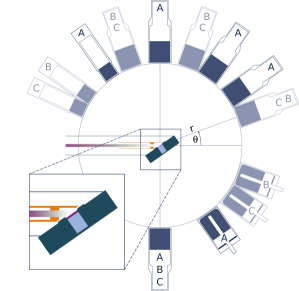
Figure 1: (Color online) Schematic cut-away view of the experimental setup. The characters denote the three different configurations (cf. Table 1). The inset shows details of the target chamber, the target (purple), electron suppression (orange), cooling water (light blue), and the beam.

Config.	LaBr3					HPGe
	$3^{\prime\prime}\!\times 3^{\prime\prime}$				$2^{\prime\prime}\!\times 2^{\prime\prime}$
A	-90∘	35∘	55∘	90∘	125∘	-55∘
B	-90∘	20∘	70∘	110∘	145∘	-20∘
C	-90∘	20∘	70∘	110∘	155∘	-35∘

Table 1: Angles covered by the $\gamma$ detectors in the three configurations. Positive angles are above the target in Fig. 1, negative angles below.

3.1 Beam line and target chamber

The irradiations have been performed at the 3 MV Tandetron accelerator of Helmholtz-Zentrum Dresden-Rossendorf, Germany [31]. The ¹H⁺ and ¹⁵N²⁺ beams were provided by a cesium sputter ion source.

The beam from the Tandetron, after being bent by 10^∘, successively passes electrostatic quadrupoles and horizontal and vertical deflector units before entering the target chamber (Fig. 1). There, about 30-50% of the beam current are absorbed on a water-cooled collimator with an opening of 5 mm diameter. The beam then passes a 30 mm long copper tube, negatively biased for secondary electron suppression, that extends to within 2 mm of the target surface (Fig. 1). The total charge impinging on the target was measured using an Ortec 439 digital current integrator connected to the electrically insulated target holder.

During the irradiations, the beam line and target chamber were kept under high vacuum, with typical pressures $(2-5)\times 10^{-7}$ mbar.

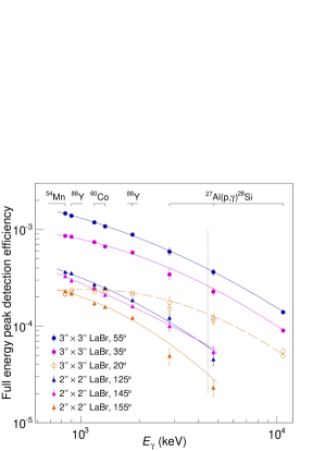
Figure 2: (Color online) $\gamma$-ray full energy peak detection efficiency data. The curves show empirical parametrizations of the efficiency curve for selected LaBr₃ detectors. The vertical dashed line corresponds to 4.439 MeV, the $\gamma$-energy of relevance for NRRA by the ¹H(¹⁵N,$\alpha\gamma$)¹²C reaction.

3.2 Targets

Two different targets have been used, each based on a tantalum backing of 27 mm diameter and 0.22 mm thickness. The targets were mounted tilted by $55^{\circ}$ with respect to the beam axis and directly watercooled during the irradiations.

For the direct kinematics measurement, a 400 nm layer of TiN was deposited by means of reactive sputtering on top of the Ta backing using gas of natural isotopic abundance containing 0.4% of the ¹⁵N isotope.

For the inverse kinematics measurement, a 300 nm layer of zirconium was evaporated on the Ta backing. Successively, hydrogen was implanted with energies of 15, 10, and 5 keV and weighted fluences of $3.3$, $1.0$, and $1.3\times 10^{17}$ atoms$/$cm², respectively [32].

3.3 Detectors

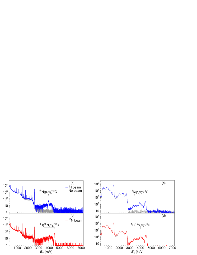
Figure 3: (Color online) $\gamma$-ray spectra on top of the resonance. HPGe detector at -55^∘, ¹H beam (a) and ¹⁵N beam (b). Arrows denote the signature of the 4439 keV $\gamma$-ray (full energy, single escape, double escape peaks). The no-beam background is shown in gray, scaled for equal livetime. LaBr₃ detector at 55^∘, ¹H beam (c) and ¹⁵N beam (d).

The emitted $\gamma$-rays were observed by six detectors. The detectors were placed in the plane of the beam, mounted atop steel bands connected to an axis below the center of the target [33]. The distance between target center and end cap of the detector was 30 cm. Altogether 12 angles and one reference angle were covered by arranging the detectors in three configurations called A, B, and C, respectively (Fig. 1, Table 1).

Four $3^{\prime\prime}\!\times 3^{\prime\prime}$ lanthanum bromide (LaBr₃, cerium doped, trade name Brillance 380) scintillation detectors, one $2^{\prime\prime}\!\times 2^{\prime\prime}$ LaBr₃, and one high-purity germanium (HPGe) detector of 100 % relative [34] efficiency were used, covering an opening angle of $14^{\circ}$, $10^{\circ}$, and $15^{\circ}$, respectively. The $3^{\prime\prime}\!\times 3^{\prime\prime}$ LaBr₃ scintillators were read out by Hamamatsu R11973 photomultiplier tubes (PMTs), the $2^{\prime\prime}\!\times 2^{\prime\prime}$ by a Hamamatsu R2038 PMT.

The first $3^{\prime\prime}\!\times 3^{\prime\prime}$ LaBr₃ was used at a fixed position of -90^∘, as a standard to connect runs in different configurations with each other. The positions of the other detectors are given in Table 1. All angles are given in the laboratory system, with respect to the direction of travel of the beam.

3.4 Electronics and data aquisition

Two different data acquisition (DAQ) systems were used: For the LaBr₃ detectors, the signals from the PMT anodes were split and the resulting two branches connected to a CAEN V965 charge-to-digital-converter (QDC) and a constant fraction discriminator (CFD), respectively. The trigger and the conversion gate for the QDC were generated in a CAEN V1495 field programmable gate array (FPGA) from the logical OR of the five CFD outputs. The dead time of the LaBr₃ DAQ system was estimated from the accepted-trigger to trigger ratio to be 2 %.

Due to the high light yield of the innovative LaBr₃ scintillator [35] and the large efficiency of the PMTs used, saturation effects changed the PMT gain for $\gamma$-ray energies above 3 MeV. For the graphical representation the pulse height data were thus re-calibrated and re-sampled to give a linear gain.

For the HPGe detector, the energy signals were amplified and shaped using an Ortec 671 spectroscopic amplifier and digitized and recorded using a histogramming Ortec 919E analog-to-digital converter (ADC) and multichannel buffer unit. A dead time of typically 0.7% was derived by the Gedcke-Hale method [36] for the HPGe DAQ.

3.5 $\gamma$-ray detection efficiency

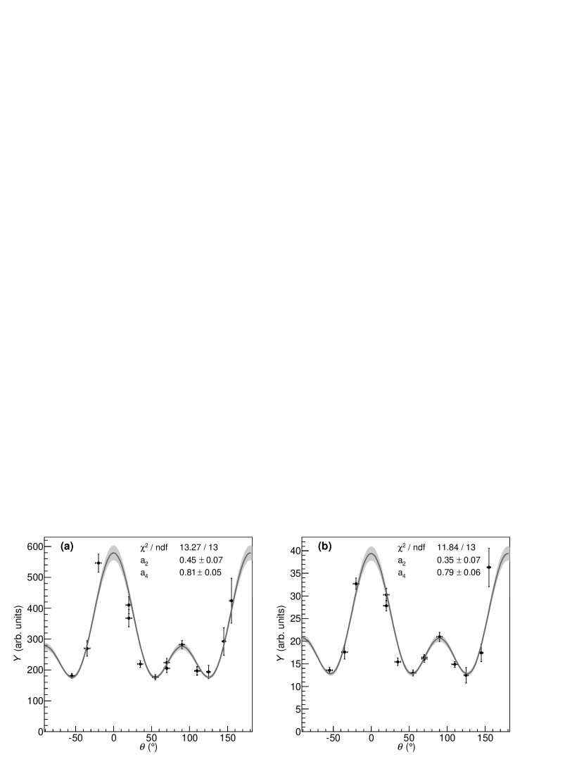
Figure 4: Angular distribution of the $\gamma$-ray yield and fit to the data for direct (a) and inverse kinematics (b). The $1\sigma$ uncertainty band of the fit is shown in gray.

For an absolute yield determination, it is important to precisely know the $\gamma$-ray detection efficiency. Therefore, instead of using calculated efficiency values with their inherent uncertainties, here a different approach is adopted [14, 37, 38]. Using calibrated radioisotope sources and nuclear reactions, the $\gamma$-ray detection efficiency is obtained up to 10.76 MeV directly from experimental data. As a first step, the full energy peak detection efficiency was determined using ⁶⁰Co, ⁵⁴Mn, and ⁸⁸Y activity standards with an activity uncertainty of 0.5%-1.0%. In order to extend the curve (Fig. 2) to higher energies, in a second step the $E_{\rm p}=992$ keV resonance of the ²⁷Al(p,$\gamma$)²⁸Si reaction was used. The well-known ratio of emission rates of the 1779- and 10764-keV $\gamma$-rays [39], the known branching ratios [40] for the $\gamma$ lines at 2839 keV and 4743 keV, and the known angular distributions [40] were used for this purpose.

For some of the $3^{\prime\prime}\!\times 3^{\prime\prime}$ detectors, the positions were kept the same in configurations B and C, in order to check the reproducibility of the efficiency curve (Fig. 2). Several example efficiency curves are shown in Fig. 2, showing generally similar slopes. The normalization is lower for the $2^{\prime\prime}\!\times 2^{\prime\prime}$ detector due to its lower active volume. At the lowest angle used here, 20^∘, the curve has a different shape due to a high amount of passive material ($\sim$6 cm of water, aluminium, and stainless steel) passed by the $\gamma$-rays.

The resulting 4439 keV efficiency from the parametric fit of the data at higher and lower $\gamma$-ray energies has 3% uncertainty for the $3^{\prime\prime}\!\times 3^{\prime\prime}$ detectors and up to 11% uncertainty, depending on the configuration, for the $2^{\prime\prime}\!\times 2^{\prime\prime}$ LaBr₃. For the HPGe detector with its better energy resolution, additional ²⁷Al(p,$\gamma$)²⁸Si lines could be used, and the efficiency uncertainty was 2% for configurations A and B and 8% for configuration C, where the ²⁷Al(p,$\gamma$)²⁸Si spectrum was accidentally overwritten.

3.6 Experimental procedure

As a first step, for a given beam (¹⁵N or ¹H), the beam energy was set to the top of the yield curve, $E_{\rm lab}(^{15}{\rm N})$ = 6.6 MeV and $E_{\rm lab}(^{1}{\rm H})$ = 0.462 MeV, respectively. Then, irradiations were performed subsequently in the three configurations A, B, and C. The beam current on target was 0.7-1.8 $\mu$A for ¹⁵N²⁺ (corrected for secondary electron effects) and 4-6  $\mu$A for ¹H⁺.

The yields from the three configurations are connected to each other by normalizing to the yield of the detector at -90^∘ that was kept at the same position throughout the experiment. Possible degradations in the target under the intense ion beam bombardment therefore affect the yield of the reference detector and the yield at the angle under study by exactly the same factor. Indeed it was found that the hydrogen implanted Zr target showed a 23% decrease of the yield at -90^∘ over the course of the experiment. Because of the normalization to the -90^∘ detector, this decrease does not affect the results. The typical irradiation time for the angular distribution measurement was several hours per data point. The TiN target, instead, remained stable under bombardment.

3.7 Interpretation of the in-beam $\gamma$-ray spectra

The observed $\gamma$-ray spectra in the HPGe detector show no significant beam-induced lines except for the ones from the reaction under study (Fig. 3). The observed $\gamma$-ray energy at the 55^∘ forward angle subtended by the HPGe in configuration B is higher in the ¹⁵N beam case than for ¹H beam. This is due to the higher Doppler shift because of the higher velocity of the center of mass for ¹⁵N beam. For the same reason, the Doppler broadening of the peak is larger.

The LaBr₃ detectors show the same general picture as the HPGe (Fig. 3). However, the LaBr₃ energy resolution is lower than for HPGe, as expected.

For the analysis of the angular distribution, only the full energy peaks were used. The laboratory background was subtracted, scaled for equal livetime. The statistical uncertainty of the resultant $\gamma$-yield was 1-5% for the $3^{\prime\prime}\!\times 3^{\prime\prime}$ LaBr₃, 2-12% for the smaller $2^{\prime\prime}\!\times 2^{\prime\prime}$ detector, and up to 3% for the HPGe.

3.8 Resulting angular distribution

The 4439 keV yields, after normalization by the $-90^{\circ}$ detector to one common scale given by configuration A, were plotted together (Fig. 4). The y axis error bars in Fig. 4 reflect the statistical uncertainty, the efficiency error, and the statistical uncertainty of the -90^∘ normalization. The x axis error bars correspond to $1/\sqrt{12}$ of the full angle subtended by the detector crystals, i.e. for the purpose of the fit it is assumed that the full angle corresponds to 92% coverage for a normal distribution.

The y axis normalization of Fig. 4 has first been determined by fitting each of the two yield curves with the parameterization

$$W(\theta)=a_{0}\left[1+a_{2}P_{2}(\cos\theta)+a_{4}P_{4}(\cos\theta)\right]$$ (7)

where $P_{2,4}$ are the second and fourth order Legendre polynomials and $a_{0,2,4}$ are parameters to be determined. Then, the arbitrary normalization is included in parameter $a_{0}$.

In a second step, for each of the two kinematics $a_{0}$ was fixed at its previously fitted value, and the fit was repeated varying $a_{2,4}$. The resulting $a_{2,4}$ parameters and their errors are shown in the insets in Fig. 4. The $a_{2,4}$ results are mutually consistent for both ¹H and ¹⁵N beams, and their weighted averages are then adopted (Table 2).

Table 2: Angular distribution coefficients $a_{2,4}$ for eq. (7). In addition, the ratio of angular corrections $W(\theta)$ is given for 90^∘ and 55^∘.

	$a_{2}$	$a_{4}$	$\displaystyle\frac{W(90^{\circ})}{W(55^{\circ})}$
Barnes et al. [10]	$0.24\pm 0.11$	$0.96\pm 0.06$	1.98
Kraus et al. [11]	0.33	0.80	1.65
Present work	$0.38\pm 0.04$	$0.80\pm 0.04$	1.60$\pm$0.06

In order to facilitate the comparison with the present data, the angular distribution coefficients given in the literature [10, 11] have been converted to the nowadays adopted Legendre parameterization (Table 2). The only inverse-kinematics work [30] did not provide the data or parameterization in numerical form but reported its data to be consistent with Kraus et al. [11].

For one pair of angles $\theta$, the ratio of the angular corrections $W(\theta)$ have also been computed (Table 2), in order to give a tangible impression of the anisotropy and facilitate the comparison. The present result is less anisotropic than what was found by Barnes et al. [10] but consistent with the Kraus et al. result [11]. Due to the smaller opening angles of the detectors used here, the present result is less prone to systematic errors than these previous works [10, 11] and should be recommended for further use.

4 Re-determination of the resonance strength

For the purposes of hydrogen depth profiling compared to a standard, it is sufficient to know that the cross section on top of the resonance is much larger than the off-resonant cross section, i.e. the ratio of resonant to off-resonant cross section. This assumption has previously been proven experimentally [30]. Recently, new data and extrapolations became available for the off-resonant cross section [41, 42, 43].

For the purposes of standardless hydrogen concentration, however, the resonant cross section $\sigma_{\rm res}$ must be known. Here, instead of $\sigma_{\rm res}$, the resonance strength $\omega\gamma$ is used.

The total width $\Gamma$ of the resonance had originally been assumed to be as high as 900 eV [44, 45]. Later it was discovered that it was much lower, of the order of 120 eV, greatly spurring interest in its use for applied physics [27]. The most precise width value to date, $\Gamma$ = $(124\pm 17)$ eV, has been obtained using a proton beam on a frozen nitrogen target [29].

For the strength, a number of previous measurements exist (Table 3). For the pre-1985 works, the experimental results given are converted to a resonance strength $\omega\gamma$ here, in order to facilitate a comparison. The quoted thick-target yield in the early work by Schardt et al. [44] has been converted here to a resonance strength using textbook [17] formulae. Hebbard [45] gives the proton and $\alpha$ widths, this is converted to $\omega\gamma$ here. The integrated $\gamma$-ray yield given by Gorodetzky et al. [46] has been converted to a strength. Leavitt et al. [15] studied several levels of interest and extracted the proton and $\alpha$-particle widths from an R-matrix fit; from these values $\omega\gamma$ has been obtained.

Zijderhand and van der Leun [12] have determined the resonance strength relative to the ¹⁵N(p,$\alpha\gamma$)¹²C resonance at $E_{\rm lab}(^{1}{\rm H})$ = 897 keV, using two Ge(Li) detectors in close geometry at 55^∘ angle. Becker et al. used a gas target, $\alpha$-particle yield measurements at one angle, and a previous $\alpha$-particle angular distribution [15] to determine the strength [13]. Marta et al. [14] measured the strength relative to the recently developed standard value [47] of $\omega\gamma_{278}$ = (13.1$\pm$0.6)$\times 10^{-3}$ eV for the $E_{\rm p}$ = 278 keV resonance in the ¹⁴N(p,$\gamma$)¹⁵O reaction.

$\omega\gamma$ [eV]		Ref.	Year	Method
26		[44]	1952	$\gamma$-ray yield measurement.
24		[45]	1960	$\gamma$-ray yield measurement.
27$\pm$	3	[46]	1968	$\gamma$-ray yield measurement.
21$\pm$	4	[15]	1983	Based on R-matrix fit.
17$\pm$	2	[12]	1986	$\gamma$-ray yield, relative to resonance at $E_{\rm p}$ = 897 keV, one angle.
21.1$\pm$	1.4	[13]	1995	$\alpha$-yield measurement, gas target, inverse kinematics, one angle.
22.7$\pm$	1.4	[14]	2010	$\gamma$-yield, relative to 14N(p,$\gamma$)15O resonance at $E_{\rm p}$ = 278 keV, one angle.
25.0$\pm$	1.5	Present		Re-analysis of data from Ref. [14], using the present angular distribution and three angles instead of one.

Table 3: Total cross section of the $E_{\rm p}$ = 430 keV resonance in the ¹⁵N(p,$\alpha\gamma$)¹²C reaction from the literature [44, 45, 46, 15, 12, 13, 14] and from the present work, expressed as resonance strength. See text for details.

Marta et al. obtained their strength based on the high-statistics yield of one detector placed in close geometry at an angle of 55^∘ with respect to the beam direction [14]. However, the yield for this close-geometry detector does not agree within one standard deviation with the predicted value using the present, newly determined angular distribution. Summarizing the four post-1980 works [15, 12, 13, 14], one uses an R-matrix fit for the strength [15], one measures the (strongly anisotropic) $\alpha$-yield at just one angle, and the final two measure the (strongly anisotropic) $\gamma$-yield at just one angle and in close geometry.

In order to improve this unsatisfactory literature situation, the resonance strength is re-determined here from the original Marta et al. data, using three detectors located at $\pm$127^∘ and 90^∘ in far geometry instead of the previous one, close-geometry detector. By using far-geometry detectors, the solid angle subtended by each detector is reduced, improving the systematic uncertainty by sacrificing some statistics. The resulting strength from this present re-analysis of the Marta et al. data is 10% higher, $\omega\gamma=(25.0\pm 1.5)$ eV (Table 3).

5 Working formula for hydrogen analyses

Table 4: Product $\eta\times W^{\prime}(\theta)$ of detection efficiency and angular correction from a GEANT4 simulation for several different detectors, angles $\theta$ to the beam direction, and distances $d$ to the target.

	$3^{\prime\prime}\!\times 3^{\prime\prime}$ BGO			$4^{\prime\prime}\!\times 4^{\prime\prime}$ BGO			$10^{\prime\prime}\!\times 10^{\prime\prime}$ NaI	$4\pi$ NaI	$4\pi$ BGO
d (mm)	10	20	30	10	20	30	70
$0^{\circ}$	0.1196	0.0877	0.0664	0.1734	0.1361	0.1091	0.1075	0.4507	0.3218
$45^{\circ}$						0.0725	0.0727
$55^{\circ}$						0.0653	0.0657
$90^{\circ}$						0.0592	0.0588
$135^{\circ}$						0.0726	0.0728

Table 5: Stopping power $\left.\frac{dE}{dx}\right|_{i}$ for $6.4$ MeV ¹⁵N^+,2+ ions in different materials $i$ from the SRIM [21] software, in units of $\rm eV/(10^{15}at/cm^{2})$.

Target $i$	Stopping power
H (solid)	61.1
Ti	445
TiN	445+195 = 640
Ta	632
Si	279
GaN	422+195 = 617

In the present section, a simple working formula for the hydrogen content in frequently investigated materials in a given NRRA setup is developed, using the full eq. (3).

The yield $Y_{\rm max}^{\infty}$ at the plateau of the resonance can be obtained by the experimental observable, the number of observed counts per unit charge (in Coulombs) on target $Y_{\rm Q}$, by

$$Y_{\rm max}^{\infty}=\frac{Y_{\rm Q}\times qe}{\eta\times W^{\prime}(\theta)}$$ (8)

where $qe$ is the electrical charge of one beam particle (typically one or two elementary charges, depending on whether ¹⁵N⁺ or ¹⁵N²⁺ beam is used), and $\eta$ the efficiency of the detector used for detecting the 4.4 MeV $\gamma$ rays. $W^{\prime}(\theta)$ is a modified form of the angular correction from eq. (7), without the normalization and corrected for the attenuation of the anisotropy by the fact that the detector is not infinitely small and thus averages over some angular range:

$$W^{\prime}(\theta)=1+a_{2}Q_{2}P_{2}(\cos\theta)+a_{4}Q_{4}P_{4}(\cos\theta)$$ (9)

In principle, the attenuation coeffients $Q_{2,4}\in[0;1]$ may be analytically calculated for simple geometries [48]. For the present purposes, they are instead determined from a Monte Carlo simulation in the GEANT4 [49] framework that directly produces the product $\eta\times W^{\prime}(\theta)$, for the detection of the full energy peak of the 4.439 MeV $\gamma$ ray (Table 4).

For detectors and geometries not included in Table 4, $\eta\times W^{\prime}(\theta)$ may be determined in two different ways. First, developing a Monte Carlo simulation describing the detector geometry, and including the un-attenuated angular distribution $W(\theta)$ from eq. (7). Second, by measuring the $\gamma$-ray detection efficiency at 4.439 MeV by using radioactive sources and nuclear reactions (sec. 3.5) and then using the attenuated angular distribution $W^{\prime}(\theta)$ from eq. (9) using calculated [48] attenuation coeffients.

The simulated values of $\eta\times W^{\prime}(\theta)$ in Table 4 have been motivated by a selection of setups at various laboratories worldwide that are used for NRRA hydrogen depth profiling with a ¹⁵N beam. Only setups with a sufficiently detailed description of the geometry were included [50, 8, 51, 52, 53, 54]. Passive materials between target and detector have been neglected:

• In Paris [50], an unshielded $4^{\prime\prime}\!\times 4^{\prime\prime}$ BGO placed at $0^{\circ}$ in 20 mm distance was used for NRRA.

• A similar setup with the same detector geometry but 30 mm distance to the sample is located at the 5 MV tandem in Tokyo [8].

• In Dresden, the AIDA2 upgrade of the AIDA setup [51] includes a $3^{\prime\prime}\!\times 3^{\prime\prime}$ BGO crystal at $0^{\circ}$ for NRRA and a 5-axes manipulator serving as sample holder enabling to use different distances to the detector.

• At the 3 MV pelletron in Göttingen [52], a low-level $\gamma$ counting setup uses a $10^{\prime\prime}\!\times 10^{\prime\prime}$ NaI(Tl) detector with anti-muon veto at $90^{\circ}$ with 70 mm distance[55] to the target.

• In Bochum [53], a $12^{\prime\prime}\!\times 12^{\prime\prime}$ $4\pi$ NaI(Tl) detector with a bore hole of 35 mm diameter and the sample in the very center [56] is used for NRRA.

• Another bore hole detector is used in Helsinki [54], comprising an annular BGO cystal of 200 mm length and 35 mm radial thickness surrounding an opening of 89 mm diameter.

In order to facilitate the discussion, an abbreviation for the constant factors included in eq. (3) is introduced, also including the elementary charge from eq. (8):

$$\varepsilon = \frac{1}{e}\left(\frac{m_{\rm H}+m_{15}}{m_{\rm H}}\frac{\lambda_{\rm res}^{2}}{2}\omega\gamma\right)$$ (10)

$$= 2.69\times 10^{13}\,\rm C^{-1}\,eV/(10^{15}at/cm^{2})$$

Equation (3) can then be expressed as:

$$n_{\rm H}=\frac{\displaystyle\sum\limits_{i}n_{i}\left.\frac{dE}{dx}\right|_{i}}{\displaystyle\frac{\varepsilon\times\eta\times W^{\prime}(\theta)}{q\times Y_{\rm Q}}-\left.\frac{dE}{dx}\right|_{\mathrm{H}}}$$ (11)

The stopping power $\left.\frac{dE}{dx}\right|_{i}$ has been tabulated here for several materials with relevance to hydrogen depth profiling (Table 5), using data from the SRIM [21] software. The uncertainty for the SRIM stopping power values of ions heavier than beryllium, thus also for ¹⁵N, has been estimated [21] to be 5.6%.

The inputs to eq. (11) are thus:

• The concentrations $n_{x}$ in atoms/cm³ of the various elements in the compound.

• Stopping powers $\left.\frac{dE}{dx}\right|_{i}$ from Table 5 or SRIM [21].

• $\varepsilon=2.69\times 10^{13}\,\rm C^{-1}\,eV/(10^{15}at/cm^{2})$, eq. (10).

• Angle-weighted efficiency $\eta\times W(\theta)$ (Table 4).

• Charge state $q$ of the beam ($q$=2 for ¹⁵N²⁺ beam).

• Experimental yield $Y_{\rm Q}$ in counts per Coulomb incident beam charge.

• Hydrogen stopping power $\left.\frac{dE}{dx}\right|_{i}$ (Table 5).

Using these values and eq. (11), the hydrogen content of a sample under study can be directly determined, without the need for a standard or an approximation requiring low hydrogen content.

6 Example hydrogen depth profiles

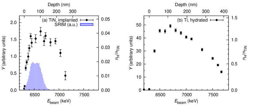
Figure 5: (Color online) Hydrogen depth profiles of (a) hydrogen implanted in TiN and (b) hydrated Ti. In panel (a), the predicted depth profile from a SRIM simulation using the implantation profile is also shown, scaled arbitrarily. The slightly non-linear behavior of the concentration scale (right y-axis) in panel (b) is caused by the stopping power of hydrogen. See text for further details.

As an illustration, hydrogen concentration data from an ongoing cross section measurement of the astrophysically relevant ¹²C(p,$\gamma$)¹³N reaction [32] are shown and analyzed in the following. In the experiment, a solid hydrogen target is irradiated with a ¹²C beam, and the $\gamma$ rays are detected with a 60% relative [34] efficiency HPGe detector placed at $55^{\circ}$ angle with respect to the beam, at a distance to the target of $d$ = 34 mm.

The challenge in that experiment is to determine the hydrogen content of the target in situ by changing the beam from ¹²C to ¹⁵N. To this end, each ¹²C irradiation is bracketed by ¹⁵N irradiations before and afterwards, allowing to judge both the relative target stability and the absolute hydrogen content quantitatively. Several different target production schemes were tried, in order to determine which target best sustains the long, high-intensity ¹²C irradiations. The parameters for eq. (11) are $q$=2 (¹⁵N²⁺ beam), $\eta\times W^{\prime}(\theta)$ = 0.00201$\pm$0.00007.

The first example used for the present study is a titanium nitride layer of 400 nm thickness that is deposited on a 0.22 mm thick tantalum carrier by the reactive sputtering technique. The TiN layer was implanted with 11 and 5 keV hydrogen ions with weighted fluences of $6.0$ and $3.4\times 10^{17}$ atoms$/$cm², respectively. The sample was cooled by liquid nitrogen during the implantation.

After significant ¹²C bombardment, the hydrogen profile of the sample is determined, using eq. (6) for the x-axis and eq. (11) for the y-axis shows a steep rising slope at the target surface and an effective width of the hydrogen profile of about 200 nm (Fig. 5, left panel). The comparison with the predicted profile from the implantation profile (using SRIM [21]) shows that the implanted hydrogen was rather mobile and diffused up to a depth of 200 nm, presumably limited by the effective target temperature at this depth, in equilibrium between heating by the ion beam and the liquid nitrogen cooling of the backing.

Table 6: Error budget for the hydrogen concentration.

Effect	Relative	Contribution
	error	to $\Delta n_{\rm H}/n_{\rm H}$    (%)
		(a) TiN	(b) Ti
Resonance strength $\omega\gamma$	6.0	6.1	7.2
$\eta\times W^{\prime}(\theta=55^{\circ})$	3.7	3.8	4.4
15N stopping in Ti and N, $\left.\frac{dE}{dx}\right|_{i}$	5.6	5.6	5.6
15N stopping in solid H, $\left.\frac{dE}{dx}\right|_{\mathrm{H}}$	5.6	0.1	1.1
Total systematic		8.4	10.2
Statistical (on the plateau)		4.6	2.1

The second example discussed here consists of a 300 nm thick layer of titanium, deposited by evaporation on a 0.22 mm thick tantalum backing. This layer was then hydrated by the following process: It was exposed to a hydrogen atmosphere (normal pressure, constant flow of 10 liters/hour) and slowly (1 K/min) heated up to 350^∘ C and held for two hours at the nominal temperature, then slowly cooled to room temperature, all the while maintaining the hydrogen flow. The sample was subsequently used for a two day long irradiation with ¹²C beam for an astrophysically motivated study [32].

The hydrogen profile was determined also for this sample (fig. 5, right panel), again after ¹²C bombardment. The absolute hydrogen level for the sample reaches a maximum stoichiometry of TiH_1.3, similar to the frequently used level of TiH_1.5 [32]. Hydrogen is seen in also beyond the Ti/Ta boundary at 300 nm, probably due to the effect of the heavy ¹²C bombardment mobilizing some hydrogen atoms. Note that the hydrogen concentration for the hydrated titanium sample would be underestimated by 11% if the stopping power of the hydrogen in eq. (11) were neglected.

The error budget is then evaluated. For case (a) shown here, relation (4) applies. For case (b) instead, the stopping by hydrogen is not negligible anymore. This latter effect leads to an over-proportional influence of the parameters $\omega\gamma$ and $\eta\times W^{\prime}(\theta=55^{\circ})$ entering $\varepsilon$ (Table 6, last column).

The resulting relative uncertainty is dominated in both examples given by the three components resonance strength (sec. 4), angular distribution (sec. 3) and efficiency, and ¹⁵N energy loss in the carrier matrix [21]. These effects lead to 8% systematic uncertainty for a sample of low hydrogen content, where approximation (4) applies, and 10% systematic uncertainty for a sample with high hydrogen content, where (4) does not hold. In both cases shown here, the statistical uncertainty is negligible when compared to the systematic uncertainty, for a typical running time of 2-3 minutes per data point on the resonance plateau for both cases shown here.

7 Discussion and summary

Hydrogen depth profiling by way of nuclear resonant reaction analysis using the ¹H(¹⁵N,$\alpha\gamma$)¹²C resonance at $E_{\rm lab}(^{15}{\rm N})$ = 6.4 MeV has been re-examined. It was shown that for samples with high hydrogen content, the textbook approach of determining the hydrogen content by scaling with the yield on a standard of known composition [4, 5, 8, 9, 6] may lead to deviations, if the stopping power contribution of the hydrogen atoms is neglected. An absolute determination of the hydrogen content is one way to correct this problem.

Subsequently, two experimental building blocks for such an absolute determination have been provided in the present work: The angular distribution of the emitted $\gamma$-rays from the ¹H(¹⁵N,$\alpha\gamma$)¹²C resonance has been measured, first with ¹H beam incident on a ¹⁵N target, then with ¹⁵N beam incident on a ¹H target (used for NRRA hydrogen depth profiling), and Legendre coefficients of $a_{2}$ = 0.38$\pm$0.04 and $a_{4}$ = 0.80$\pm$0.04 have been derived from the data. Subsequently, the absolute resonance strength has been re-determined to be (25.0$\pm$1.5) eV.

Finally, a simple working formula for absolute hydrogen depth profile determination has been developed based on the new data and applied to two examples. The present approach and formula are limited to cases where either Bragg’s stopping power addition rule holds, or where deviations can be quantified. For cases with unknown deviations to Bragg’s stopping power rule, an additional uncertainty has to be taken into account.

Two examples show that this approach can yield hydrogen profiles with 8-10% systematic uncertainty, depending on the actual hydrogen concentration. This absolute error bar is higher than the 2% reproducibility which has been reported previously in an intercomparison exercise involving a low concentration sample [57]. It is mainly due to the remaining uncertainty in the resonance strength and in the stopping power. Even still, it is hoped that these data and considerations prove to be useful for cases of high hydrogen concentrations and wherever the use of standards is difficult.

References

References

- [1] Y. Fukai, The Metal-Hydrogen System. Basic Bulk Properties, 2nd Edition, Springer, Berlin, Heidelberg, New York, 2005.
- [2] A. Züttel, A. Borgschulte, L. Schlapbach (Eds.), Hydrogen as a Future Energy Carrier, WILEY-VCH Verlag, Weinheim, 2008.
- [3] F. Ding, B. I. Yakobson, Challenges in hydrogen adsorptions: from physisorption to chemisorption, Front. Phys. 6 (2) (2011) 142–150.
- [4] P. K. Khabibullaev, B. G. Skorodumov, Determination of hydrogen in materials: nuclear physics methods, Springer, Berlin and Heidelberg, 1989.
- [5] G. Schatz, A. Weidinger, Nuclear condensed matter physics: nuclear methods and applications, Wiley, Chichester, 1996.
- [6] M. Nastasi, J. W. Meyer, Y. Wang, Ion Beam Analysis, CRC Press, Boca Raton, Florida, 2015.
- [7] W. M. Mueller, J. P. Blackledge, G. G. Libowitz (Eds.), Metal Hydrides, Academic Press, New York and London, 1968.
- [8] M. Wilde, K. Fukutani, Hydrogen detection near surfaces and shallow interfaces with resonant nuclear reaction analysis, Surface Science Reports 69 (4) (2014) 196 – 295.
- [9] Y. Wang, M. Nastasi (Eds.), Handbook of Modern Ion Beam Materials Analysis, 2nd Edition, Vol. 2 of , Materials Research Society, Warendale, Pennsylvania, 2009.
- [10] C. A. Barnes, D. B. James, G. C. Neilson, Angular Distribution of the Gamma Rays from the Reaction , Can. J. Phys. 30 (1952) 717–718.
- [11] A. A. Kraus, A. P. French, W. A. Fowler, C. C. Lauritsen, Angular Distribution of Gamma-Rays and Short-Range Alpha-Particles from N15(p, )C12, Phys. Rev. 89 (1) (1953) 299–301.
- [12] F. Zijderhand, C. van der Leun, Strong M2 transitions, Nucl. Phys. A 460 (1986) 181–200.
- [13] H. Becker, M. Bahr, M. Berheide, L. Borucki, M. Buschmann, C. Rolfs, G. Roters, S. Schmidt, W. Schulte, G. Mitchell, J. Schweitzer, Hydrogen depth profiling using 18O ions, Z. Phys. A 351 (1995) 453–465.
- [14] M. Marta, E. Trompler, D. Bemmerer, R. Beyer, C. Broggini, A. Caciolli, M. Erhard, Z. Fülöp, E. Grosse, G. Gyürky, R. Hannaske, A. R. Junghans, R. Menegazzo, C. Nair, R. Schwengner, T. Szücs, S. Vezzú, A. Wagner, D. Yakorev, Resonance strengths in the 14N(p,)15O and 15N(p,)12C reactions, Phys. Rev. C 81 (2010) 055807.
- [15] R. A. Leavitt, H. C. Evans, G. T. Ewan, H. Mak, R. E. Azuma, C. Rolfs, K. P. Jackson, Isospin mixing in 2- levels in 16O, Nucl. Phys. A 410 (1983) 93–102.
- [16] W. A. Fowler, C. C. Lauritsen, T. Lauritsen, Gamma-Radiation from Excited States of Light Nuclei, Rev. Mod. Phys. 20 (1948) 236–277.
- [17] C. Iliadis, Nuclear Physics of Stars, Wiley-VCH, Weinheim, 2007.
- [18] W. H. Bragg, R. Kleeman, On the Particles of Radium, and their Loss of Range in passing through various Atoms and Molecules, Phil. Mag. 10 (1905) 318–340.
- [19] D. I. Thwaites, Review of stopping powers in organic materials, Nucl. Inst. Meth. B 27 (1987) 293–300.
- [20] J. F. Ziegler, J. M. Manoyan, The stopping of ions in compounds, Nucl. Inst. Meth. B 35 (1988) 215–228.
- [21] J. F. Ziegler, M. D. Ziegler, J. P. Biersack, SRIM - The stopping and range of ions in matter (2010), Nucl. Inst. Meth. B 268 (2010) 1818–1823.
- [22] R. Mikšová, A. Macková, P. Malinský, V. Hnatowicz, P. Slepička, The stopping powers and energy straggling of heavy ions in polymer foils, Nucl. Inst. Meth. B 331 (2014) 42–47.
- [23] Y. Zhang, W. J. Weber, Validity of Bragg’s rule for heavy-ion stopping in silicon carbide, Phys. Rev. B 68 (23) (2003) 235317.
- [24] Y. Zhang, W. J. Weber, D. A. Grove, J. Jensen, G. Possnert, Electronic stopping powers for heavy ions in niobium and tantalum pentoxides, Nucl. Inst. Meth. B 250 (2006) 62–65.
- [25] M. Zier, U. Reinholz, H. Riesemeier, M. Radtke, F. Munnik, Accurate stopping power determination of 15N ions for hydrogen depth profiling by a combination of ion beams and synchrotron radiation, Nucl. Inst. Meth. B 273 (2012) 18–21.
- [26] W. A. Lanford, H. P. Trautvetter, J. F. Ziegler, J. Keller, New precision technique for measuring the concentration versus depth of hydrogen in solids, Appl. Phys. Lett. 28 (1976) 566.
- [27] B. Maurel, G. Amsel, A new measurement of the 429 keV 15N(p,)12C resonance. Applications of the very narrow width found to 15N and 1H depth location: I. Resonance width measurement, Nucl. Inst. Meth. 218 (1-3) (1983) 159–164.
- [28] M. Zinke-Allmang, S. Kalbitzer, M. Weiser, Vibrational doppler-broadening of inverse p,gamma reaktions on hydrogen bearing targets, Z. Phys. A 320 (1985) 697–698.
- [29] T. Osipowicz, K. P. Lieb, S. Brüssermann, Frozen target measurements of the 430 keV 15N(p,) resonance, Nucl. Inst. Meth. B 18 (1987) 232–235.
- [30] K. M. Horn, W. A. Lanford, Measurement of the off-resonance cross section of the 6.4 MeV nuclear reaction, Nucl. Inst. Meth. B 34 (1988) 1–8.
- [31] M. Friedrich, W. Bürger, D. Henke, S. Turuc, The Rossendorf 3 MV tandetron: a new generation of high-energy implanters, Nucl. Inst. Meth. A 382 (1996) 357–360.
- [32] K. Stöckel, T. P. Reinhardt, S. Akhmadaliev, D. Bemmerer, S. Gohl, S. Reinicke, K. Schmidt, M. Serfling, T. Szücs, M. Takács, L. Wagner, K. Zuber, S-factor measurement of the (,) reaction in inverse kinematics, EPJ Web Conf. 93 (2015) 03012.
- [33] M. Dietz, et al., Angular distribution of rays from inelastic neutron scattering, in: Nuclear Energy Agency, NEA Nuclear Data Week, Institut Curie, Paris, 2015.
- [34] G. Gilmore, Practical -ray spectrometry, 2nd edition, John Wiley and Sons, New York, 2008.
- [35] G. F. Knoll, Radiation Detection and Measurement, 4th Edition, John Wiley & Sons, New York, 2010.
- [36] R. Jenkins, R. W. Gould, D. Gedcke, Quantitative X-ray spectrometry, Marcel Dekker, New York and Basel, 1981, Ch. 4.8.5, pp. 266–271.
- [37] K. Schmidt, S. Akhmadaliev, M. Anders, D. Bemmerer, K. Boretzky, A. Caciolli, D. Degering, M. Dietz, R. Dressler, Z. Elekes, Z. Fülöp, G. Gyürky, R. Hannaske, A. R. Junghans, M. Marta, M.-L. Menzel, F. Munnik, D. Schumann, R. Schwengner, T. Szücs, A. Wagner, D. Yakorev, K. Zuber, Resonance triplet at =4.5 MeV in the 40Ca(,)44Ti reaction, Phys. Rev. C 88 (2) (2013) 025803.
- [38] R. Depalo, F. Cavanna, F. Ferraro, A. Slemer, T. Al-Abdullah, S. Akhmadaliev, M. Anders, D. Bemmerer, Z. Elekes, G. Mattei, S. Reinicke, K. Schmidt, C. Scian, L. Wagner, Strengths of the resonances at 436, 479, 639, 661, and 1279 keV in the 22Ne(p,)23Na reaction, Phys. Rev. C 92 (2015) 045807.
- [39] F. Zijderhand, F. P. Jansen, C. Alderliesten, C. van der Leun, Detector-efficiency calibration for high-energy gamma-rays, Nucl. Inst. Meth. A 286 (3) (1990) 490 – 496.
- [40] A. Anttila, J. Keinonen, M. Hautala, I. Forsblom, Use of the 27Al(p,)28Si, = 992 keV resonance as a gamma-ray intensity standard, Nucl. Inst. Meth. 147 (3) (1977) 501 – 505.
- [41] M. Wilde, K. Fukutani, Evaluation of non-resonant background in hydrogen depth profiling via 1H( 15N,) 12C nuclear reaction analysis near 13.35 MeV, Nucl. Inst. Meth. B 232 (2005) 280–284.
- [42] G. Imbriani, R. J. deBoer, A. Best, M. Couder, G. Gervino, J. Görres, P. J. LeBlanc, H. Leiste, A. Lemut, E. Stech, F. Strieder, E. Uberseder, M. Wiescher, Measurement of rays from 15N(p,)16O cascade and 15N(p,1)12C reactions, Phys. Rev. C 85 (6) (2012) 065810.
- [43] G. Imbriani, R. J. deBoer, A. Best, M. Couder, G. Gervino, J. Görres, P. J. LeBlanc, H. Leiste, A. Lemut, E. Stech, F. Strieder, E. Uberseder, M. Wiescher, Erratum: Measurement of rays from 15N(p,)16O cascade and 15N(p,1)12C reactions [Phys. Rev. C 85, 065810 (2012)], Phys. Rev. C 86 (3) (2012) 039902(E).
- [44] A. Schardt, W. A. Fowler, C. A. Lauritsen, The disintegration of N15 by protons, Phys. Rev. 86 (1952) 527–536.
- [45] D. F. Hebbard, Proton capture by N15, Nucl. Phys. 15 (1960) 289–315.
- [46] S. Gorodetzky, J. C. Adloff, F. Brochard, P. Chevallier, D. Dispier, P. Gorodetzky, R. Modjtahed-Zadeh, F. Scheibling, Cascades - de quatre résonances de la réaction 15N(p,)16O, Nucl. Phys. A 113 (1968) 221–232.
- [47] E. Adelberger, A. García, R. G. H. Robertson, K. A. Snover, A. B. Balantekin, K. Heeger, M. J. Ramsey-Musolf, D. Bemmerer, A. Junghans, C. A. Bertulani, J.-W. Chen, H. Costantini, P. Prati, M. Couder, E. Uberseder, M. Wiescher, R. Cyburt, B. Davids, S. J. Freedman, M. Gai, D. Gazit, L. Gialanella, G. Imbriani, U. Greife, M. Hass, W. C. Haxton, T. Itahashi, K. Kubodera, K. Langanke, D. Leitner, M. Leitner, P. Vetter, L. Winslow, L. E. Marcucci, T. Motobayashi, A. Mukhamedzhanov, R. E. Tribble, K. M. Nollett, F. M. Nunes, T.-S. Park, P. D. Parker, R. Schiavilla, E. C. Simpson, C. Spitaleri, F. Strieder, H.-P. Trautvetter, K. Suemmerer, S. Typel, Solar fusion cross sections. II. The pp chain and CNO cycles, Rev. Mod. Phys. 83 (2011) 195–246.
- [48] M. E. Rose, The analysis of angular correlation and angular distribution data, Phys. Rev. 91 (3) (1953) 610–615.
- [49] S. Agostinelli, et al., GEANT 4 - a simulation toolkit, Nucl. Inst. Meth. A 506 (2003) 250–303.
- [50] G. Amsel, E. d’Artemare, G. Battistig, E. Girard, L. Gosset, P. Révész, Narrow nuclear resonance position or cross section shape measurements with a high precision computer controlled beam energy scanning system, Nucl. Inst. Meth. B 136-138 (1998) 545–550.
- [51] M. O. Liedke, W. Anwand, R. Bali, S. Cornelius, M. Butterling, T. T. Trinh, A. Wagner, S. Salamon, D. Walecki, A. Smekhova, H. Wende, K. Potzger, Open volume defects and magnetic phase transition in Fe60Al40 transition metal aluminide, J. Appl. Phys. 117 (16) (2015) 163908.
- [52] M. Uhrmacher, M. Schwickert, H. Schebela, K.-P. Lieb, Miss MaRPel - a 3 MV pelletron accelerator for hydrogen depth profiling, J. Alloys Comp. 404-406 (2005) 307–311, proceedings of the 9th International Symposium on Metal-Hydrogen Systems, Fundamentals and Applications (MH2004) The International Symposium on Metal-Hydrogen Systems, Fundamentals and Applications, MH2004.
- [53] F. Traeger, M. Kauer, C. Wöll, D. Rogalla, H.-W. Becker, Analysis of surface, subsurface, and bulk hydrogen in ZnO using nuclear reaction analysis, Phys. Rev. B 84 (2011) 075462.
- [54] P. Torri, J. Keinonen, K. Nordlund, A low-level detection system for hydrogen analysis with the reaction , Nuclear Instruments and Methods in Physics Research Section B: Beam Interactions with Materials and Atoms 84 (1) (1994) 105 – 110.
- [55] H. Damjantschitsch, M. Weiser, G. Heusser, S. Kalbitzer, H. Mannsperger, An in-beam-line low-level system for nuclear reaction -rays, Nuclear Instruments and Methods in Physics Research 218 (1-3) (1983) 129–140.
- [56] A. Spyrou, H.-W. Becker, A. Lagoyannis, S. Harissopulos, C. Rolfs, Cross-section measurements of capture reactions relevant to the p process using a -summing method, Phys. Rev. C 76 (2007) 015802.
- [57] G. Boudreault, R. G. Elliman, R. Grötzschel, S. C. Gujrathi, C. Jeynes, W. N. Lennard, E. Rauhala, T. Sajavaara, H. Timmers, Y. Q. Wang, T. D. M. Weijers, Round Robin: measurement of H implantation distributions in Si by elastic recoil detection, Nucl. Inst. Meth. B 222 (2004) 547–566.