Geometric Dominating-Set and Set-Cover via Local-Search

Abstract

In this paper, we study two classic optimization problems: minimum geometric dominating set and set cover. In the dominating-set problem, for a given set of objects in the plane as input, the objective is to choose a minimum number of input objects such that every input object is dominated by the chosen set of objects. Here, one object is dominated by another if both of them have a nonempty intersection region. For the second problem, for a given set of points and objects in a plane, the objective is to choose a minimum number of objects to cover all the points. This is a special version of the set-cover problem.

Both problems have been well studied subject to various restrictions on the input objects. These problems are APX-hard for object sets consisting of axis-parallel rectangles, ellipses, $\displaystyle\alpha$-fat objects of constant description complexity, and convex polygons. On the other hand, PTASs (polynomial time approximation schemes) are known for object sets consisting of disks or unit squares. Surprisingly, a PTAS was unknown even for arbitrary squares.

For both problems obtaining a PTAS remains open for a large class of objects.

For the dominating-set problem, we prove that a popular local-search algorithm leads to an $\displaystyle(1+\varepsilon)$ approximation for object sets consisting of homothetic set of convex objects (which includes arbitrary squares, $\displaystyle k$-regular polygons, translated and scaled copies of a convex set, etc.) in $\displaystyle n^{O(1/\varepsilon^{2})}$ time. On the other hand, the same technique leads to a PTAS for geometric covering problem when the objects are convex pseudodisks (which includes disks, unit height rectangles, homothetic convex objects, etc.). As a consequence, we obtain an easy to implement approximation algorithm for both problems for a large class of objects, significantly improving the best known approximation guarantees.

1 Introduction

1.1 Problems Studied

We consider two fundamental combinatorial optimization problems in a geometric context, dominating-set and set-cover. Let $\displaystyle\cal P$ be a subset of the real plane $\displaystyle\mathbb{R}^{2}$, and let $\displaystyle\mathscr{S}$ be a collection of subsets of $\displaystyle\cal P$, called objects. A subset $\displaystyle\mathscr{S}^{\prime}\subseteq\mathscr{S}$ is a dominating-set if every element of $\displaystyle\mathscr{S}$ has a nonempty intersection with at least one element of $\displaystyle\mathscr{S}^{\prime}$. A subset $\displaystyle\mathscr{S}^{\prime\prime}\subseteq\mathscr{S}$ is a cover if every point of $\displaystyle\cal P$ lies within at least one element of $\displaystyle\mathscr{S}^{\prime\prime}$. The dominating-set and set-cover problems involve computing a minimum cardinality dominating-set and set-cover, respectively. Both problems have a wealth of theoretical results and practical applications. Geometric set-cover problem has many application in real world for example wireless sensor networks, optimizing number of stops in an existing transportation network, job scheduling [2, 7, 17].

1.2 Local Search

It is well known that both of these problems are NP-hard in the most general setting, and hence researchers have focused on approximation algorithms. In this paper, we analyze an approach based on local search. Local search is a popular heuristic algorithm. This is an iterative algorithm which starts with a feasible solution and improves the solution after each iteration until a locally optimal solution is reached. One big advantage of local search is that it is very easy to implement and easy to parallelize [8]. As mentioned by Cohen-Addad and Mathieu [8], it is interesting to analyze such algorithms even when alternative, theoretically optimal polynomial-time algorithms are known.

1.3 Our Results

Our results on the dominating-set problem apply under the assumption that the input consists of homothets of a convex body in the plane, that is, the elements of $\displaystyle\mathscr{S}$ are equal to each other up to translation and positive uniform scaling. This includes a large class of natural object sets, such as collections of squares of arbitrary size, collections of regular $\displaystyle k$-gons of arbitrary size, and collections of circular disks of arbitrary radii. First, we show that the standard local search algorithm leads to a polynomial time approximation scheme (PTAS) for computing a minimum dominating-set of homothetic convex objects. For the analysis, we use a separator-based technique, which was introduced independently by Chan and Har-Peled [4] and Mustafa and Ray [29]. The main part of this proof technique is to show the existence of a planar graph satisfying a locality condition (to be defined in Section 2.1). Gibson et al. [16] used the same paradigm where the objects were arbitrary disks. Inspired by their work, we ask whether we can generalize their framework to more general objects. Our result on the dominating-set problem can be viewed as a non-trivial generalization of their result. To show the planarity, first, we decompose (or shrink) a set of homothetic convex objects (which are returned by the optimum algorithm and the local search algorithm) into a set of interior disjoint objects so that each input object has a “trace” in this new set of objects. This decomposition is motivated from the idea of core decomposition introduced by Mustafa et al. [28], and this technique could be of independent interest. Next, we consider the nearest-site Voronoi diagram for this set of disjoint objects with respect to the well-known convex distance function. The decomposition ensures that each site has a nonempty cell in the Voronoi diagram. Finally, we show that the dual of this Voronoi diagram satisfies the locality condition. Note that if homothets of a centrally symmetric convex object are given, then one can avoid the disjoint decomposition, and the analysis is much simpler.

Our results on the set-cover problem apply under the assumption that the input consists of a collection of convex pseudodisks in the plane. A set of objects is said to be a collection of pseudodisks, if the boundaries of every pair of them intersect at most twice. Note that this generalizes collections of homothets. We use a similar technique as the previous one. First, we show that we can decompose (or shrink) a set of pseudodisks (which are returned by the optimum algorithm and the local search algorithm) into a set of interior disjoint objects so that each input point has a “trace” in this new set of objects. We consider a graph $\displaystyle{\cal G}$ in which each vertex corresponds to a shrunken object, and two vertices are joined by an edge if the corresponding objects share an edge in their boundary. Since the shrunken objects are interior disjoint with each other, the graph $\displaystyle{\cal G}$ is planar. We prove that the graph $\displaystyle{\cal G}$ satisfies the locality condition.

Given $\displaystyle\varepsilon>0$, a $\displaystyle(1+\varepsilon)$-approximation algorithm for the dominating-set (resp., set-cover) problem returns a dominating-set (resp., set-cover) whose cardinality is larger than the optimum by a factor of at most $\displaystyle(1+\varepsilon)$. Our results are given below.

Theorem 1.

Given a set $\displaystyle\mathscr{S}$ of n convex homothets in $\displaystyle\mathbb{R}^{2}$ and $\displaystyle\varepsilon>0$, there exists a $\displaystyle(1+\varepsilon)$ approximation algorithm for dominated set based on local search that runs in time $\displaystyle n^{O(1/\varepsilon^{2})}$.

Theorem 2.

Given a set $\displaystyle\mathscr{S}$ of n convex pseudodisks in $\displaystyle\mathbb{R}^{2}$ and $\displaystyle\varepsilon>0$, there exists a $\displaystyle(1+\varepsilon)$ approximation algorithm for set-cover based on local search that runs in time $\displaystyle n^{O(1/\varepsilon^{2})}$.

1.4 Related Works

Our work is motivated by recent progress on approximability of various fundamental geometric optimization problems like finding maximum independent sets [1], minimum hitting set of geometric intersection graphs [29], and minimum geometric set covers [28].

Dominating-Set: The minimum dominating-set problem is NP-complete for general graphs [15]. From the result of Raz and Safra [30], it follows that it is NP-hard even to obtain a $\displaystyle(c\log\Delta)$-approximate dominating-set for general graphs, where $\displaystyle\Delta$ is the maximum degree of a node in the graph and $\displaystyle c\,(>0)$ is any constant (see [24]).

Researchers have studied the problem for different graph classes like planar graphs, intersection graphs, bounded arboricity graphs, etc. Recently, Har-Peled and Quanrud [18] proved that local search produces a PTAS for graphs with polynomially bounded expansion. Gibson and Pirwani [16] gave a

PTAS for the intersection graphs of arbitrary disks. Unless $\displaystyle P=NP$ [9], it is not possible to compute a $\displaystyle((1-\epsilon)\ln n)$-approximate dominating-set in polynomial time for $\displaystyle n$ homothetic polygons [13, 20, 31]. Erlebach and van Leeuwen [11] proved that the problem is APX-hard for the intersection graphs of axis-parallel rectangles, ellipses, $\displaystyle\alpha$-fat objects of constant description complexity, and of convex polygons with $\displaystyle r$-corners ($\displaystyle r\geq 4$), i.e., there is no PTAS for these unless $\displaystyle P=NP$.

Effort has been devoted to related problems involving various objects such as squares, regular polygons, etc.. Marx [26] proved that the problem is $\displaystyle W[1]$-hard for unit squares, which implies that no efficient-polynomial-time-approximation-scheme (EPTAS) is possible unless $\displaystyle FPT=W[1]$ [27]. The best known approximation factor for homothetic $\displaystyle 2k$-regular polygons is $\displaystyle O(k)$ due to Erlebach and van Leeuwen [11], where $\displaystyle k>0$. They also obtained an $\displaystyle O(k^{2})$-approximation algorithm for homothetic $\displaystyle(2k+1)$-regular polygons. Even worse, for the homothetic convex polygons where each polygons has $\displaystyle k$-corners, the best known result is $\displaystyle O(k^{4})$-approximation. Currently, there is no PTAS even for arbitrary squares. We consider the problem for a set of homothetic convex objects.

Set-Cover: The set-cover problem is known to be NP-complete [21]. The geometric variant has received a great amount of attention due to its wide applications (for example the recent breakthrough of Bansal and Pruhs [2]). Unfortunately, the geometric version of the problem also remains NP-complete even when the objects are unit disks or unit squares [3, 19].

Erlebach and van Leeuwen [12] obtained a PTAS for the geometric set-cover problem when the objects are unit squares. Recently, Chan and Grant [3] showed that the problem is APX-hard when the objects are axis-aligned rectangles. They extended the results to several other classes of objects including axis-aligned ellipses in $\displaystyle\mathbb{R}^{2}$, axis-aligned slabs, downward shadows of line segments, unit balls in $\displaystyle\mathbb{R}^{3}$, axis-aligned cubes in $\displaystyle\mathbb{R}^{3}$. A QPTAS was developed by Mustafa et. al. [28] for the problem when the objects are pseudodisks. The current state of the art lacks a PTAS when the objects are pseudodisks which includes a large class of objects: arbitrary squares, arbitrary regular polygons, homothetic convex objects.

In the weighted setting, Varadarajan introduced the idea of quasi-uniform sampling to obtain an $\displaystyle O(\log\phi(OPT))$-approximation guarantees in the weighted setting for a large class of objects for which such guarantees were known in the unweighted case [32]. Here $\displaystyle\phi(OPT)$ is the union complexity of the objects in the optimum set $\displaystyle OPT$. Very recently, Li and Jin proposed a PTAS for the weighted version of the problem when the objects are unit disks [25].

In [17], the authors described a PTAS for the problem of computing a minimum cover of given points by a set of weighted fat objects, by allowing them to expand by some $\displaystyle\delta$-fraction. A multi-cover variant of the problem (where each point is covered by at least k sets) under geometric settings was studied in [5].

1.5 Organization

In Section 2, we present a general algorithm based on the local search technique. For the sake of completeness, we present a high-level view of the analysis technique of local search which was introduced by Chan & Har-Peled [4] and Mustafa & Ray [29]. In Section 3, we prove two results for a set of pseudodisks which are common tools for analyzing both dominating-set and geometric set-cover problem. Thereafter, in Section 4 and Section 5 we prove the locality condition for the dominating-set prolem when the objects are homothets of a convex polygon and of a centrally symmetric convex polygon, respectively. In Section 6, we prove the locality condition for the geometric set-cover problem when the objects are convex pseudodisks.

1.6 Notation and Preliminaries

Throughout the paper, we use capital letters to denote objects and caligraphic font to denote sets of objects. We make the general-position assumption that if two objects of the input set have a nonempty intersection, then their interiors intersect. No three object boundaries intersect in a common point. We denote the set $\displaystyle\{1,2,\ldots,n\}$ as $\displaystyle[n]$. By a geometric object (or object, in short) $\displaystyle R$, we refer to a simply connected compact region in $\displaystyle\mathbb{R}^{2}$ with nonempty interior. In other words, the object $\displaystyle R$ is a closed region bounded by a closed Jordan curve $\displaystyle\partial{R}$. The $\displaystyle\operatorname{int}(R)$ is defined as all the points in $\displaystyle R$ which do not appear in the boundary $\displaystyle\partial{R}$. Given two objects $\displaystyle U$ and $\displaystyle V$, we say that $\displaystyle U$ has an interior overlap with $\displaystyle V$ if $\displaystyle\operatorname{int}(U)\cap\operatorname{int}(V)\neq\emptyset$, and given a set of objects $\displaystyle\mathcal{V}$, we say that $\displaystyle U$ has an interior overlap with $\displaystyle\mathcal{V}$ if $\displaystyle U$ has an interior overlap with any $\displaystyle V\in\mathcal{V}$.

For a set of objects $\displaystyle\cal R$, we define the cover-free region of any object $\displaystyle R_{i}\in{\cal R}$ as $\displaystyle\operatorname{CF}(R_{i},{\cal R})=\bigcap_{\begin{subarray}{c}R_{j}\in{\cal R}\\ R_{j}\neq R_{i}\end{subarray}}R_{i}\setminus R_{j}$. Note that $\displaystyle\operatorname{CF}(R_{i},{\cal R})\cap R_{j}=\emptyset$ for all $\displaystyle R_{i},R_{j}(i\neq j)\in{\cal R}$. When the underlying set of objects $\displaystyle\cal R$ is obvious, we use the term $\displaystyle\operatorname{CF}(R_{i})$ instead of $\displaystyle\operatorname{CF}(R_{i},{\cal R})$. A collection of geometric objects $\displaystyle\cal R$ is said to form a family of pseudodisks if the boundary of any two objects cross each other at most twice. A collection of geometric objects $\displaystyle\cal R$ is said to be cover-free if no object $\displaystyle R\in{\cal R}$ is covered by the union of the objects in $\displaystyle{\cal R}\setminus R$, in other words, $\displaystyle\operatorname{CF}(R,{\cal R})\neq\emptyset$ for all objects in $\displaystyle\cal R$. Two objects are homothetic to each other if one object can be obtained from the other by scaling and translating.

Consider the convex distance function with respect to a convex object $\displaystyle C$ with a fixed interior point as center as follows.

Definition 1.

Given $\displaystyle p_{1},p_{2}\in\mathbb{R}^{2}$, convex distance function induced by $\displaystyle C$, denoted by $\displaystyle\delta_{C}(p_{1},p_{2})$, is the smallest $\displaystyle\alpha\geq 0$ such that $\displaystyle p_{1},p_{2}\in\alpha C$ while the center of $\displaystyle C$ is at $\displaystyle p_{1}$.

It was first introduced by Minkowski in 1911 [22, 6]. Note that this function satisfies the following properties.

Property 1.

1. The function $\displaystyle\delta_{C}$ is symmetric (i.e., $\displaystyle\delta_{C}(p_{1},p_{2})=\delta_{C}(p_{2},p_{1})$) if and only if $\displaystyle C$ is centrally symmetric.

2. Let $\displaystyle p_{1}$ and $\displaystyle p_{3}$ be any two points in $\displaystyle\mathbb{R}^{2}$ and let $\displaystyle p_{2}$ be any point on the line segment $\displaystyle\overline{p_{1}p_{3}}$, then $\displaystyle\delta_{C}(p_{1},p_{3})=\delta_{C}(p_{1},p_{2})+\delta_{C}(p_{2},p_{3})$.

3. The distance function $\displaystyle\delta_{C}$ follows the triangular inequality, i.e., and $\displaystyle\delta_{C}(p_{1},p_{3})\leq\delta_{C}(p_{1},p_{2})+\delta_{C}(p_{2},p_{3})$, where $\displaystyle p_{1}$, $\displaystyle p_{2}$ and $\displaystyle p_{3}$ are any three points in $\displaystyle\mathbb{R}^{2}$.

2 Local-Search Algorithm

We use a standard local search algorithm [29] as given in Algorithm 1.

Input: A set of $\displaystyle n$ objects $\displaystyle\mathscr{S}$ in $\displaystyle\mathbb{R}^{2}$ and a parameter $\displaystyle b$

1 Initialize $\displaystyle{\cal A}$ to an arbitrary subset of $\displaystyle\mathscr{S}$ which is a feasible solution;

2 while $\displaystyle\exists$ $\displaystyle{\cal X}\subseteq{\cal A}$ of size at most $\displaystyle b$, and $\displaystyle{\cal X}^{\prime}\subseteq\mathscr{S}$ of size at most $\displaystyle|{\cal X}|-1$ such that $\displaystyle({\cal A}\setminus{\cal X})\cup{\cal X}^{\prime}$ is a feasible solution do

3       set $\displaystyle{\cal A}\leftarrow({\cal A}\setminus{\cal X})\cup{\cal X}^{\prime}$;

4      

5Report $\displaystyle{\cal A}$;

Algorithm 1 Local-Search($\displaystyle\mathscr{S},b$)

A subset of objects $\displaystyle{\cal A}\subseteq\mathscr{S}$ is referred to $\displaystyle b$-locally optimal if one cannot obtain a smaller feasible solution by removing a subset $\displaystyle{\cal X}\subseteq{\cal A}$ of size at most $\displaystyle b$ from $\displaystyle{\cal A}$ and replacing that with a subset of size at most $\displaystyle|{\cal X}|-1$ from $\displaystyle\mathscr{S}\setminus{\cal A}$. Our algorithm computes a $\displaystyle b$-locally optimal set of objects for $\displaystyle b=\frac{\alpha}{\epsilon^{2}}$, where $\displaystyle\alpha>0$ is a suitably large constant. Observe that at the end of the while-loop, the set $\displaystyle\cal A$ is $\displaystyle b$-locally optimal, and the set $\displaystyle\cal A$ is cover-free.

Since the size of $\displaystyle{\cal A}$ is decreased by at least one after each update in Line 3, the number of iterations of the while-loop is at most $\displaystyle n$, and each iteration takes $\displaystyle O(n^{b})$ time as it needs to check every subset of size at most $\displaystyle b$. So, this while-loop needs $\displaystyle O(n^{b+1})$ time. Thus, total time complexity of the above algorithm is $\displaystyle O(n^{b+1})$.

2.1 Analysis of Approximation

We will be analyzing the algorithm’s performance with respect to both problems. When there is a difference, we will indicate the specific context within which the analysis is being performed (set-cover or dominating-set). Let $\displaystyle{\cal O}$ be the optimal solution and $\displaystyle{\cal A}$ be the solution returned by our local search algorithm. Note that both $\displaystyle{\cal O}$ and $\displaystyle{\cal A}$ ensure the following.

Claim 1.

For any object $\displaystyle A\in{\cal A}$ (resp., $\displaystyle O\in{\cal O}$), $\displaystyle\operatorname{CF}(A,{\cal A})$ (resp., $\displaystyle\operatorname{CF}(O,{\cal O})$) is nonempty. In other words, $\displaystyle{\cal A}$ (resp., $\displaystyle{\cal O}$) is cover-free.

We can assume that no object $\displaystyle S\in\mathscr{S}$ is properly contained in any other object of $\displaystyle\mathscr{S}$. We can ensure this by an initial pass over the input objects in which we remove any object of the input that is contained within another object. Thus, we can assume that there is no object $\displaystyle S\in\mathscr{S}\setminus{\cal A}$ which completely contains any object of $\displaystyle{\cal A}$. Similarly, we can assume that no object in $\displaystyle{\cal O}$ is completely contained in any object from $\displaystyle\mathscr{S}\setminus{\cal O}$. Let $\displaystyle{\cal A}^{\prime}={\cal A}\setminus{\cal O}$, $\displaystyle{\cal O}^{\prime}={\cal O}\setminus{\cal A}$.

In the context of the dominating-set problem, let $\displaystyle\mathscr{S}^{\prime}\subset\mathscr{S}$ be the set containing all objects of $\displaystyle\mathscr{S}$ which are not dominated by any object in $\displaystyle{\cal A}\cap{\cal O}$. Note that there does not exist an object $\displaystyle O\in{\cal O}^{\prime}$ which covers $\displaystyle\operatorname{CF}(A_{1},{\cal A}^{\prime})\cup\operatorname{CF}(A_{2},{\cal A}^{\prime})$, $\displaystyle A_{1},A_{2}\in{\cal A}^{\prime}$, otherwise local search would replace $\displaystyle A_{1}$ and $\displaystyle A_{2}$ by $\displaystyle O$. Similarly, there does not exist an object $\displaystyle A\in{\cal A}^{\prime}$ which covers $\displaystyle\operatorname{CF}(O_{1},{\cal O}^{\prime})\cup\operatorname{CF}(O_{2},{\cal O}^{\prime})$, $\displaystyle O_{1},O_{2}\in{\cal A}^{\prime}$ otherwise it would contradict the optimality of $\displaystyle{\cal O}$.

Now we are going to eliminate the same number of objects from both $\displaystyle{\cal A}^{\prime}$ and $\displaystyle{\cal O}^{\prime}$ to ensure that for any $\displaystyle A\in{\cal A}^{\prime}$, $\displaystyle\operatorname{CF}(A,{\cal A}^{\prime})$ is not properly contained in any object in $\displaystyle{\cal O}^{\prime}$. Let $\displaystyle O\in{\cal O}^{\prime}$ be an object that properly contains $\displaystyle\operatorname{CF}(A,{\cal A}^{\prime})$ for an object $\displaystyle A\in{\cal A}^{\prime}$. Let $\displaystyle\mathscr{S}^{\prime\prime}$ be the the set containing all objects of $\displaystyle\mathscr{S}^{\prime}$ which are not dominated by $\displaystyle O$. Note that both the sets $\displaystyle{\cal A}^{\prime}\setminus A$ and $\displaystyle{\cal O}^{\prime}\setminus O$ dominates $\displaystyle\mathscr{S}^{\prime\prime}$. We reset $\displaystyle\mathscr{S}^{\prime}\leftarrow\mathscr{S}^{\prime\prime}$. We remove $\displaystyle A$ and $\displaystyle O$ from $\displaystyle{\cal A}^{\prime}$ and $\displaystyle{\cal O}^{\prime}$, respectively by updating $\displaystyle{\cal A^{\prime}}\leftarrow{\cal A}^{\prime}\setminus A$ and $\displaystyle{\cal O}^{\prime}\leftarrow{\cal O}^{\prime}\setminus O$. We repeat this until there does not exist any object $\displaystyle O\in\cal{O}^{\prime}$ that properly contains an object $\displaystyle A\in{\cal A}^{\prime}$.

Similarly, if there exists an object $\displaystyle A\in{\cal A}^{\prime}$ that properly contains $\displaystyle\operatorname{CF}(O,{\cal O}^{\prime})$ for an object $\displaystyle O\in{\cal O}^{\prime}$, we update $\displaystyle{\cal A}^{\prime}\leftarrow{\cal A}^{\prime}\setminus A$ and $\displaystyle{\cal O}^{\prime}\leftarrow{\cal O}^{\prime}\setminus O$. Let $\displaystyle\mathscr{S}^{\prime\prime}$ be the the set containing all objects of $\displaystyle\mathscr{S}^{\prime}$ which are not dominated by $\displaystyle A$. We reset $\displaystyle\mathscr{S}^{\prime}\leftarrow\mathscr{S}^{\prime\prime}$. We repeat this until there does not exist any object $\displaystyle A\in{\cal A}^{\prime}$ that properly contains $\displaystyle\operatorname{CF}(O,{\cal O}^{\prime})$ for an object $\displaystyle O\in{\cal O}^{\prime}$. This ensures the following.

Claim 2.

For any object $\displaystyle A\in{\cal A}^{\prime}$ (resp., $\displaystyle O\in{\cal O}^{\prime}$), $\displaystyle\operatorname{CF}(A,{\cal A}^{\prime})$ (resp., $\displaystyle\operatorname{CF}(O,{\cal O}^{\prime})$) is not properly contained in any object in $\displaystyle{\cal O}^{\prime}$ (resp., $\displaystyle{\cal A}^{\prime}$).

Observe that $\displaystyle|\cal{O}\setminus\cal{O}^{\prime}|=|\cal{A}\setminus\cal{A}^{\prime}|$. Finally, we will show that $\displaystyle|{\cal A}^{\prime}|\leq(1+\epsilon)|{\cal O}^{\prime}|$ which implies that $\displaystyle|{\cal A}|\leq(1+\epsilon)|{\cal O}|$.

In the context of geometric covering, we do the similar process as discussed above to ensure Claim 2. Here, let $\displaystyle{\cal P}^{\prime}$ be the set containing all points of $\displaystyle\cal P$ which are covered by object in $\displaystyle{\cal A}^{\prime}\cap{\cal O}^{\prime}$.

Henceforth, $\displaystyle{\cal A}^{\prime},{\cal O}^{\prime},{\cal P}^{\prime}$ and $\displaystyle\mathscr{S}^{\prime}$ will be denoted as $\displaystyle{\cal A},{\cal O},{\cal P}$ and $\displaystyle\mathscr{S}$, respectively, satisfying both Claim 1 and 2.

In Sections 4.3 and 6, we prove locality conditions for the dominating-set and set-cover problems, respectively. These conditions are presented in Lemmas 1 and 2, respectively.

Lemma 1 (Locality Condition for Dominating-Set).

There exists a planar graph $\displaystyle{\cal G}=({\cal A}\cup{\cal O},{\cal E})$ such that for all $\displaystyle S\in\mathscr{S}$, if $\displaystyle S$ is dominated by at least one object of $\displaystyle\cal A$ and at least one object of $\displaystyle\cal O$, then there exists $\displaystyle A\in{\cal A}$ and $\displaystyle O\in{\cal O}$ both of which dominate $\displaystyle S$ and $\displaystyle(A,O)\in{\cal E}$.

Lemma 2 (Locality Condition for Set-Cover).

There exists a planar graph $\displaystyle{\cal G}=({\cal A}\cup{\cal O},{\cal E})$ such that for all points $\displaystyle p\in{\cal P}$, if $\displaystyle p$ is covered by at least one object of $\displaystyle\cal A$ and at least one object of $\displaystyle\cal O$, then there exists $\displaystyle A\in{\cal A}$ and $\displaystyle O\in{\cal O}$ both of which cover $\displaystyle p$ and $\displaystyle(A,O)\in{\cal E}$.

Once we have established both of these locality condition lemmas, the analysis of the algorithm is same as in [29]. For the sake of completeness, we provide the following analysis. As the graph $\displaystyle{\cal G}$ is planar, the following planar separator theorem can be used.

Theorem 3 (Frederickson [14]).

For any planar graph $\displaystyle{\cal G}=({\cal V},{\cal E})$ with $\displaystyle n$ vertices and a parameter $\displaystyle 1\leq r\leq n$, there is a set $\displaystyle{\cal X}\subseteq{\cal V}$ of size at most $\displaystyle\frac{c_{1}n}{\sqrt{r}}$, such that $\displaystyle{\cal V}\setminus{\cal X}$ can be partitioned into $\displaystyle\lceil n/r\rceil$ sets $\displaystyle{\cal V}_{1},{\cal V}_{2},\ldots{\cal V}_{\lceil n/r\rceil}$ satisfying (i) $\displaystyle|{\cal V}_{i}|\leq c_{2}r$, (ii) $\displaystyle N({\cal V}_{i})\cap{\cal V}_{j}=\emptyset$ for $\displaystyle i\neq j$, and $\displaystyle|N({\cal V}_{i})\cap{\cal X}|\leq c_{3}\sqrt{r}$, where $\displaystyle c_{1},c_{2},c_{3}>0$ are constants, and $\displaystyle N({\cal V}^{\prime})=\{U\in{\cal V}\setminus{\cal V}^{\prime}\mid\exists V\in{\cal V}^{\prime}\text{ with }(U,V)\in{\cal E}\}$.

We apply Theorem 3 to the graphs described in Lemmas 1 and 2, setting $\displaystyle r=b/c_{2}$, where $\displaystyle c_{2}$ is the constant of Theorem 3. Here, $\displaystyle n=|{\cal A}|+|{\cal O}|$ and $\displaystyle r=c_{4}/\epsilon^{2}$, for some constant $\displaystyle c_{4}$. So, $\displaystyle|{\cal V}_{i}|\leq b$. Let $\displaystyle{\cal A}_{i}={\cal A}\cap{\cal V}_{i}$ and $\displaystyle{\cal O}_{i}={\cal O}\cap{\cal V}_{i}$. Note that we must have

$$\displaystyle|{\cal A}_{i}|\leq|{\cal O}_{i}|+|N({\cal V}_{i})\cap{\cal X}|,$$ (1)

otherwise our local search would continue to replace $\displaystyle{\cal A}_{i}$ by $\displaystyle{\cal O}_{i}\cup N({\cal V}_{i})$ , resulting in a better solution. For a suitable constant $\displaystyle c_{5}$, we now have rcl’s —A— & ≤ —X—+ ∑_i—A_i— (Each element of $\displaystyle{\cal Q}$ either belongs to $\displaystyle{\cal A}_{i}$ or $\displaystyle{\cal X}$)
≤ —X— + ∑_i—O_i—+ ∑_i—N(V_i)∩X— (Follows from Equation 1)
≤ —O— + —X— + ∑_i—N(V_i)∩X— ($\displaystyle{\cal O}_{i}$ are disjoint subsets of $\displaystyle{\cal O}$)
≤ —O— + c5(—A—+—O—)b ($\displaystyle\sum\limits_{i}|N({\cal V}_{i})\cap{\cal X}|\leq\lceil{n/r}\rceil(c_{3}\sqrt{r})$ and $\displaystyle|{\cal X}|\leq c_{1}(|{\cal A}|+|{\cal O}|)/\sqrt{r}$ )
—A— ≤ 1+c5/b1-c5/b—O— (By rearranging)
—A— ≤ (1+ϵ)—O— ($\displaystyle b$ is large enough constant times $\displaystyle\frac{1}{\epsilon^{2}}$).

3 Tools for Constructing Disjoint Objects

In this section, we present two tools (or Lemmata) which are essential for analyzing our main results. An important step in our analysis (and particularly in the construction of the planar graph of Section 2.1) involves replacing a collection of overlapping objects that cover a given region with a collection of non-overlapping objects that cover the same region. This leads to the notion of a decomposition. The decomposition, we define here, is inspired by the idea of core decomposition introduced by Mustafa et al. [28].

Definition 2.

Given a set of convex objects $\displaystyle{\cal R}=\{R_{1},\ldots,R_{n}\}$, a set $\displaystyle\widetilde{\cal R}=\{{{\widetilde{R}}_{1}},\ldots,{{\widetilde{R}}_{n}}\}$ of convex objects is called a sub-decomposition if for each $\displaystyle i\in[n]$, $\displaystyle{{\widetilde{R}}_{i}}\subseteq R_{i}$. Such a set $\displaystyle\widetilde{\cal R}$ is called a decomposition if the same region is covered, that is, $\displaystyle\bigcup_{i\in[n]}{{\widetilde{R}}_{i}}=\bigcup_{i\in[n]}R_{i}$. We refer $\displaystyle{\widetilde{R}}_{i}$ as the trace of $\displaystyle R_{i}$, $\displaystyle i\in[n]$. Further, if the elements of $\displaystyle\widetilde{\cal R}$ have pairwise disjoint interiors, the decomposition/sub-decomposition is said to be disjoint.

First, we prove the following lemma which is a reminiscent of [28, Lem 3.3]. Edelsbrunner [10] introduced a very similar decomposition in the context of Euclidean disks.

Lemma 3.

For a cover-free set of convex pseudodisks $\displaystyle{\cal R}=\{R_{1},\ldots,R_{n}\}$, there exist a disjoint decomposition $\displaystyle\widetilde{\cal R}=\{{{\widetilde{R}}_{1}},\ldots,{{\widetilde{R}}_{n}}\}$ such that $\displaystyle\operatorname{CF}(R_{j},{\cal R})\subseteq{{\widetilde{R}}_{j}}$, for all $\displaystyle j\in[n]$.

Proof.

The proof is constructive. The algorithm to construct a disjoint decomposition $\displaystyle\widetilde{\cal R}=\{{{\widetilde{R}}_{1}},\ldots,{{\widetilde{R}}_{n}}\}$ of $\displaystyle{\cal R}=\{R_{1},\ldots,R_{n}\}$ is as follows. This is an $\displaystyle n$-phase algorithm. After the $\displaystyle i^{th}$ phase, the following invariants are maintained, for all $\displaystyle i\in[n]$.

Invariant 1.

The objects in $\displaystyle\widetilde{\cal R}^{i}=\{{{\widetilde{R}}_{1}}^{i},\ldots,{{\widetilde{R}}_{n}}^{i}\}$ form a decomposition of $\displaystyle{\cal R}=\{R_{1},\ldots,R_{n}\}$ such that (i) $\displaystyle\operatorname{CF}(R_{j})\subseteq{{\widetilde{R}}_{j}}^{i}$ for all $\displaystyle j\in[n]$, and (ii) $\displaystyle\operatorname{int}({{\widetilde{R}}_{t}}^{i})\cap\operatorname{int}({{\widetilde{R}}_{q}}^{i})=\emptyset$ where $\displaystyle t\neq q$ and $\displaystyle 1\leq t\leq i$, $\displaystyle 1\leq q\leq n$.

Invariant 2.

The objects in $\displaystyle\widetilde{\cal R}^{i}=\{{{\widetilde{R}}_{1}}^{i},\ldots,{{\widetilde{R}}_{n}}^{i}\}$ form a collection of convex pseudodisks.

We initialize $\displaystyle\widetilde{\cal R}^{0}={\cal R}$. This satisfies both invariants. At the beginning of the $\displaystyle i^{th}$ phase, we set $\displaystyle X=\widetilde{R}_{i}^{i-1}$. Let $\displaystyle{\cal R}_{\pi}^{i}=\{{{\widetilde{R}}_{\pi(1)}}^{i-1},\ldots,{{\widetilde{R}}_{\pi(\ell)}}^{i-1}\}$, $\displaystyle 0\leq\ell<n$ be the set of objects in $\displaystyle\widetilde{\cal R}^{i-1}$ that intersect $\displaystyle\operatorname{int}({{\widetilde{R}}_{i}}^{i-1})$. In other words, $\displaystyle\operatorname{int}({{\widetilde{R}}_{i}}^{i-1})\cap\operatorname{int}({{\widetilde{R}}_{\pi(j)}}^{i-1})\neq\emptyset$ for any $\displaystyle\pi(j)\in\Pi$, where $\displaystyle\Pi=\{\pi(1),\ldots,\pi(\ell)\}$.

Consider any object $\displaystyle{{\widetilde{R}}_{\pi(j)}}^{i-1}\in{\cal R}_{\pi}^{i}$. As $\displaystyle{{\widetilde{R}}_{\pi(j)}}^{i-1}$ and $\displaystyle X$ are pseudodisks, their respective boundaries intersect in two points. Let $\displaystyle p_{1}$ and $\displaystyle p_{2}$ be these two intersection points. By convexity, the line segment $\displaystyle\overline{p_{1}p_{2}}$ is contained in both $\displaystyle{{\widetilde{R}}_{\pi(j)}}^{i-1}$ and $\displaystyle X$. Let $\displaystyle{\cal C}_{1}$ (respectively, $\displaystyle{\cal C}_{2}$) be the part of the boundary of $\displaystyle{{\widetilde{R}}_{\pi(j)}}^{i-1}$ (respectively, $\displaystyle X$) that lie inside $\displaystyle X$ (respectively, $\displaystyle{{\widetilde{R}}_{\pi(j)}}^{i-1}$). We replace both $\displaystyle{\cal C}_{1}$ and $\displaystyle{\cal C}_{2}$ by the line segment $\displaystyle\overline{p_{1}p_{2}}$. In this way, we obtain new convex objects $\displaystyle{{\widetilde{R}}_{\pi(j)}}^{i}\subseteq{{\widetilde{R}}_{\pi(j)}}^{i-1}$ and $\displaystyle X_{j}\subseteq X$ that have interiors that are pairwise disjoint with each other, and $\displaystyle{{\widetilde{R}}_{\pi(j)}}^{i}\cup X_{j}={{\widetilde{R}}_{\pi(j)}}^{i-1}\cup X$. See Figure 1 for illustration.

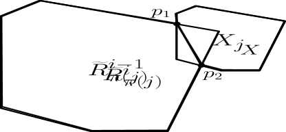
Figure 1: Illustration of Lemma 3.

For all $\displaystyle\pi(j)\in\Pi$, we construct the corresponding $\displaystyle{{\widetilde{R}}_{\pi(j)}}^{i}$ as above. At the end of this phase, we assign $\displaystyle{{\widetilde{R}}_{i}}^{i}=\bigcap_{j\in\Pi}X_{j}$. Note that $\displaystyle{{\widetilde{R}}_{i}}^{i}$ is also convex as it is intersection of some convex objects. We set $\displaystyle{{\widetilde{R}}_{j}}^{i}={{\widetilde{R}}_{j}}^{i-1}$ for all $\displaystyle j(\neq i)\in[n]\setminus\Pi$. As a result, we obtain a collection of convex objects $\displaystyle\widetilde{\cal R}^{i}$.

Observe that, for any point $\displaystyle p$ that is contained in the union of $\displaystyle{\cal R}_{\pi}^{i}$, either there exists a $\displaystyle j$ such that this point lies within $\displaystyle{{\widetilde{R}}_{\pi(j)}}^{i}$, and so is covered by this set, or it lies within $\displaystyle X_{j}$ for all $\displaystyle j$, and hence it lies within their common intersection, which is $\displaystyle X$. So, $\displaystyle\widetilde{\cal R}^{i}$ is a decomposition of $\displaystyle\widetilde{\cal R}^{i-1}$.

Thus, after the $\displaystyle i^{th}$ phase, we find a decomposition $\displaystyle\widetilde{\cal R}^{i}$ such that $\displaystyle\operatorname{int}({{\widetilde{R}}_{i}}^{i})\cap\operatorname{int}({{\widetilde{R}}_{j}}^{i})=\emptyset$ for all $\displaystyle j(\neq i)\in\{1,\ldots,n\}$. On the other hand, we have $\displaystyle\operatorname{int}({{\widetilde{R}}_{t}}^{i-1})\cap\operatorname{int}({{\widetilde{R}}_{q}}^{i-1})=\emptyset$ where $\displaystyle t\neq q$ and $\displaystyle 1\leq t\leq i-1$, $\displaystyle 1\leq q\leq n$. Combining these, we obtain $\displaystyle\operatorname{int}({{\widetilde{R}}_{t}}^{i})\cap\operatorname{int}({{\widetilde{R}}_{q}}^{i})=\emptyset$ where $\displaystyle t\neq q$ and $\displaystyle 1\leq t\leq i$, $\displaystyle 1\leq q\leq n$.

Since the union of objects in $\displaystyle\widetilde{\cal R}^{i}$ is same as the union of the objects in $\displaystyle\widetilde{\cal R}^{i-1}$, and the objects in $\displaystyle\widetilde{\cal R}^{i-1}$ are cover-free, so each object $\displaystyle{{\widetilde{R}}_{j}}^{i}$ has its cover-free region $\displaystyle\operatorname{CF}(R_{j})$ which is not covered by others, for all $\displaystyle j\in[n]$. Thus, Invariant 1 is maintained. Now, we prove that Invariant 2 is also maintained. We prove the objects in $\displaystyle\widetilde{\cal R}^{i}$ form pseudodisks by showing the following claim.

Claim 3.

$\displaystyle\widetilde{\cal R}^{i}$ is a collection of convex pseudodisks.

(a) Case 1

(a) *

(b) Case 2

(b) *

(c) Case 3

(c) *

Before Phase $\displaystyle i$

(a) Case 1

(d) *

(b) Case 2

(e) *

(c) Case 3

(f) *

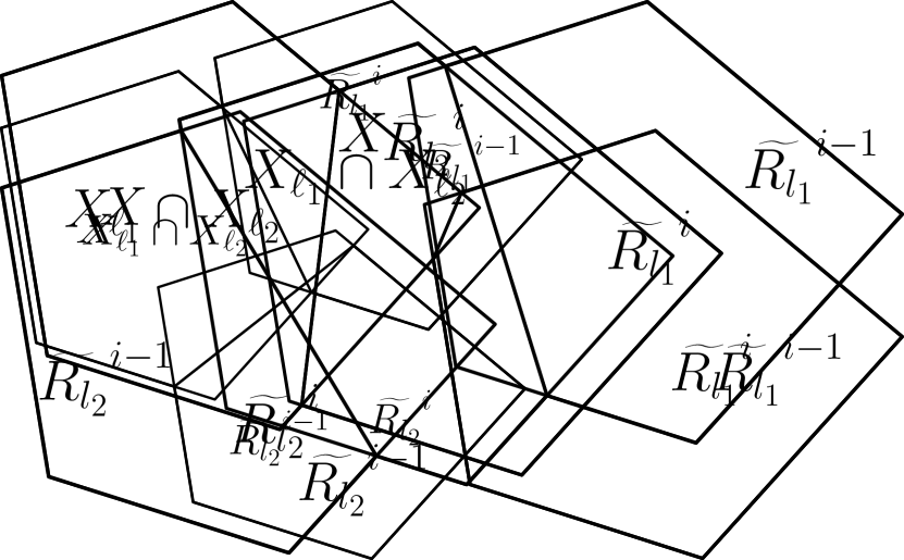
After Phase $\displaystyle i$

Figure 2: Illustration of Claim 3.

Proof.

It suffices to show that for any two objects $\displaystyle{{\widetilde{R}}_{\ell_{1}}}^{i-1}$ and $\displaystyle{{\widetilde{R}}_{\ell_{2}}}^{i-1}$ in $\displaystyle{R~{}}^{i-1}$, their boundaries $\displaystyle\partial{{\widetilde{R}}_{\ell_{1}}}^{i}$ and $\displaystyle\partial{{\widetilde{R}}_{\ell_{2}}}^{i}$ can cross each other at most twice.

Recall the definition of $\displaystyle X$ from the above construction. For any $\displaystyle R\in{\cal R}_{\pi}^{i}$, let $\displaystyle I(R)$ be the interval $\displaystyle R\cap\partial X$ on the boundary of $\displaystyle X$. Due to the Invariant 1, no pseudodisk in $\displaystyle\widetilde{\cal R}^{i-1}$ is completely contained in another pseudodisk, so the intervals are well defined.

There are three possible cases:

• Case 1: $\displaystyle I({{\widetilde{R}}_{\ell_{1}}}^{i-1})\cap I({{\widetilde{R}}_{\ell_{2}}}^{i-1})=\emptyset$,

• Case 2: $\displaystyle I({{\widetilde{R}}_{\ell_{1}}}^{i-1})\subseteq I({{\widetilde{R}}_{\ell_{2}}}^{i-1})$,

• Case 3: $\displaystyle I({{\widetilde{R}}_{\ell_{1}}}^{i-1})\cap I({{\widetilde{R}}_{\ell_{2}}}^{i-1})\neq\emptyset$ and $\displaystyle I({{\widetilde{R}}_{\ell_{1}}}^{i-1})\nsubseteq I({{\widetilde{R}}_{\ell_{2}}}^{i-1})$.

In both Case 1 and Case 2 (see Figure 2(a) and (b)), $\displaystyle\partial{{\widetilde{R}}_{\ell_{1}}}^{i}$ and $\displaystyle\partial{{\widetilde{R}}_{\ell_{2}}}^{i}$ do not have any new crossing which $\displaystyle\partial{{\widetilde{R}}_{\ell_{1}}}^{i-1}$ and $\displaystyle\partial{{\widetilde{R}}_{\ell_{2}}}^{i-1}$ did not have. In fact they may lost intersections lying in $\displaystyle X$. As $\displaystyle\partial{{\widetilde{R}}_{\ell_{1}}}^{i-1}$ and $\displaystyle\partial{{\widetilde{R}}_{\ell_{2}}}^{i-1}$ may cross each other at most twice, so does $\displaystyle\partial{{\widetilde{R}}_{\ell_{1}}}^{i}$ and $\displaystyle\partial{{\widetilde{R}}_{\ell_{2}}}^{i}$. In Case 3 (see Figure 2(c)), $\displaystyle\partial{{\widetilde{R}}_{\ell_{1}}}^{i-1}$ and $\displaystyle\partial{{\widetilde{R}}_{\ell_{2}}}^{i-1}$ crosses each other once in $\displaystyle X$ and once outside $\displaystyle X$. The outside crossing remains same for $\displaystyle\partial{{\widetilde{R}}_{\ell_{1}}}^{i}$ and $\displaystyle\partial{{\widetilde{R}}_{\ell_{2}}}^{i}$, and they cross each other once along new part of their boundaries, i.e., along the boundary of $\displaystyle X_{\ell_{1}}\cap X_{\ell_{2}}$. Thus, the claim follows.

∎

After completion of the $\displaystyle n^{th}$ phase, we assign $\displaystyle\widetilde{\cal R}=\widetilde{\cal R}^{n}$. The proof of the lemma follows from the Invariant 1. ∎

Now, we prove the following important lemma which we use as a tool for obtaining disjoint sub-decompositions. The previous lemma is used to obtain disjoint decomposition when the objects are pseudodisks. When the set of objects does not satisfy the pseudodisk property, but they are shrunken from a set of of pseudodisks, we apply the following tool to obtain a disjoint sub-decomposition.

Lemma 4.

Given two sets $\displaystyle{\cal U}$ and $\displaystyle{\cal V}$ of distinct convex objects such that their union forms a collection of pseudodisks, let $\displaystyle{{\cal U}^{0}}$ and $\displaystyle{{\cal V}^{0}}$ be any disjoint sub-decompositions of $\displaystyle{\cal U}$ and $\displaystyle{\cal V}$, respectively. Let $\displaystyle U_{i}$ and $\displaystyle V_{j}$ be any two convex pseudodisks from $\displaystyle{\cal U}$ and $\displaystyle{\cal V}$, respectively, and $\displaystyle{U^{0}_{i}}$ and $\displaystyle{V^{0}_{j}}$ be two corresponding convex objects from $\displaystyle{{\cal U}^{0}}$ and $\displaystyle{{\cal V}^{0}}$, respectively, such that $\displaystyle\operatorname{CF}({U^{0}_{i}},{{\cal U}^{0}}\cup{{\cal V}^{0}})\neq\emptyset$, $\displaystyle\operatorname{CF}({V^{0}_{j}},{{\cal U}^{0}}\cup{{\cal V}^{0}})\neq\emptyset$ and $\displaystyle\operatorname{int}({U^{0}_{i}})\cap\operatorname{int}({V^{0}_{j}})\neq\emptyset$. Then we can find $\displaystyle{U^{0}_{ij}}\subseteq{U^{0}_{i}}$ and $\displaystyle{V^{0}_{ji}}\subseteq{V^{0}_{j}}$ such that the following properties are satisfied.

• $\displaystyle{U^{0}_{ij}}$ and $\displaystyle{V^{0}_{ji}}$ are convex, have nonempty disjoint interiors, and their intersection consists of a separating line segment, which we denote by $\displaystyle E^{0}_{ij}$.

• $\displaystyle{U^{0}_{i}}\setminus{U^{0}_{ij}}$ is completely contained in $\displaystyle V_{j}$.

• $\displaystyle{V^{0}_{j}}\setminus{V^{0}_{ji}}$ is completely contained in $\displaystyle U_{i}$.

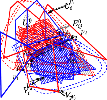
Figure 3: Petals: tiled regions are Petals of $\displaystyle U_{i}^{0}$; $\displaystyle\operatorname{NCpetal}$s are marked with red.

Proof.

Given two convex objects $\displaystyle U$ and $\displaystyle V$, define a petal of $\displaystyle U$ with respect to $\displaystyle V$ to be a connected component of $\displaystyle U\setminus V$. Since $\displaystyle U_{i}^{0}$ and $\displaystyle V_{j}^{0}$ need not be pseudodisks, there may be multiple petals of $\displaystyle U_{i}^{0}$ with respect to $\displaystyle V_{j}^{0}$. Let us assume that there are $\displaystyle k$ such petals, which we denote by $\displaystyle\operatorname{Petal}_{t}(U_{i}^{0})$, for $\displaystyle 1\leq t\leq k$. Thus, $\displaystyle U_{i}^{0}\setminus V_{j}^{0}=\bigcup_{t=1}^{k}\operatorname{Petal}_{t}(U_{i}^{0})$. Similarly, we define $\displaystyle\operatorname{Petal}(V_{j}^{0})$ to be the set of petals of $\displaystyle V_{j}^{0}$ with respect to $\displaystyle U_{i}^{0}$ , and we let $\displaystyle k^{\prime}$ denote their number. Observe that each petal is bounded by two boundary arcs, one from $\displaystyle\partial U_{i}^{0}$ and the other from $\displaystyle\partial V_{j}^{0}$ (see Figure 3). Also observe that consecutive petals are defined by consecutive intersection points between the boundaries of the two objects.

Since $\displaystyle V^{0}_{j}\subseteq V_{j}$, we have $\displaystyle{U^{0}_{i}}\setminus V_{j}\subseteq{U^{0}_{i}}\setminus{V^{0}_{j}}$. Define $\displaystyle\operatorname{NCpetal}({U^{0}_{i}})$ to be the subset of petals of $\displaystyle U_{i}^{0}$ (with respect to $\displaystyle V_{j}^{0}$) that are not entirely covered by $\displaystyle V_{j}$, that is, $\displaystyle\operatorname{NCpetal}({U^{0}_{i}})=\{\operatorname{Petal}_{t}({U^{0}_{i}})\in\{{U^{0}_{i}}\setminus{V^{0}_{j}}\}|\operatorname{Petal}_{t}({U^{0}_{i}})\cap\{{U^{0}_{i}}\setminus V_{j}\}\neq\emptyset\}$. Similarly, we define $\displaystyle\operatorname{NCpetal}({V^{0}_{j}})$. Because $\displaystyle\operatorname{CF}({U^{0}_{i}},{{\cal U}^{0}}\cup{{\cal V}^{0}})\neq\emptyset$, $\displaystyle\operatorname{NCpetal}({U^{0}_{i}})$ contains at least one element, and the same holds for $\displaystyle\operatorname{NCpetal}({V^{0}_{j}})$ (see Figure 3).

Consider only the uncovered petals (that is, $\displaystyle\operatorname{NCpetal}(U_{i}^{0})\cup\operatorname{NCpetal}(V^{0}_{j})$). Let us label the petals of $\displaystyle\operatorname{NCpetal}(U_{i}^{0})$ with the letter “u” and label the petals of $\displaystyle\operatorname{NCpetal}(V^{0}_{j})$ with the letter “v”. Let $\displaystyle R^{0}_{ij}={U^{0}_{i}}\cap{V^{0}_{j}}$. If you consider the cyclic order of these petals around $\displaystyle\partial R^{0}_{ij}$, the alternating pattern “u…v…u…v” cannot occur in the cyclic sequence as shown in the following argument (see Figure 4).

• Suppose to the contrary that the alternating pattern “u…v…u…v” occurs in the cyclic sequence. Then there must exist points $\displaystyle u_{1},u_{2}$ (from the first and third “u” petals in the sequence) that lie in $\displaystyle U_{i}^{0}\setminus V^{0}_{j}$. Similarly, there exist points $\displaystyle v_{1},v_{2}$ (from the second and fourth “v” petals) that lie in $\displaystyle V^{0}_{j}\setminus U_{i}^{0}$. Because of the alternation, the line segments $\displaystyle\overline{u_{1}u_{2}}$ and $\displaystyle\overline{v_{1}v_{2}}$ intersect in $\displaystyle R^{0}_{ij}$. However, the existence of these two line segments violates the hypothesis that $\displaystyle U_{i}$ and $\displaystyle V_{j}$ are pseudodisks.

Since the alternation pattern “u…v…u…v” cannot arise in the cyclic sequence, it follows the cyclic order of uncovered petals around $\displaystyle\partial R^{0}_{ij}$ consists of a sequence of petals from $\displaystyle\operatorname{NCpetal}(U^{0}_{i})$ followed by a sequence from $\displaystyle\operatorname{NCpetal}(V^{0}_{j})$. As a result, we can find a line segment $\displaystyle\overline{p_{1}p_{2}}$ lying in $\displaystyle\operatorname{int}(R^{0}_{ij})$ whose two endpoints are on $\displaystyle\partial R^{0}_{ij}$ such that all the uncoverd petals of $\displaystyle U^{0}_{i}$ (formally $\displaystyle\operatorname{NCpetal}(U^{0}_{i})$) lie on one side of this line segment and the uncoverd petals of $\displaystyle V^{0}_{j}$ (formally $\displaystyle\operatorname{NCpetal}(V^{0}_{j})$) lie on the other side. In other words, extension of this line segment $\displaystyle\overline{p_{1}p_{2}}$ partitions the plane into two half-spaces $\displaystyle{\mathcal{H}}^{0}_{i}$ and $\displaystyle{\mathcal{H}}^{0}_{j}$ where $\displaystyle{\mathcal{H}}^{0}_{i}$ contains all the petals of $\displaystyle\operatorname{NCpetal}({U^{0}_{i}})$ and $\displaystyle{\mathcal{H}}^{0}_{j}$ contains all the petals of $\displaystyle\operatorname{NCpetal}({V^{0}_{j}})$. We define $\displaystyle{U^{0}_{ij}}={\mathcal{H}}^{0}_{i}\cap{U^{0}_{i}}$ and $\displaystyle{V^{0}_{ji}}={\mathcal{H}}^{0}_{j}\cap{V^{0}_{j}}$. The line segment $\displaystyle\overline{{p}_{1}{p}_{2}}$ plays the role of the separating line segment $\displaystyle E^{0}_{ij}$. Claim (i) follows because $\displaystyle{p}_{1}$ and $\displaystyle{p}_{2}$ lie on the boundary of both $\displaystyle U_{i}^{0}$ and $\displaystyle V_{j}^{0}$. Claim (ii) follows because $\displaystyle U_{i}^{0}\setminus U_{ij}^{0}$ consists a portion of $\displaystyle R_{ij}^{0}$ (which clearly lies in $\displaystyle V_{j}$) together with a subset of petals of $\displaystyle U_{i}^{0}$ that are all covered by $\displaystyle V_{j}$ . Claim (iii) is symmetrical. Hence $\displaystyle{U^{0}_{ij}}$, $\displaystyle{V^{0}_{ij}}$ satisfy the lemma.

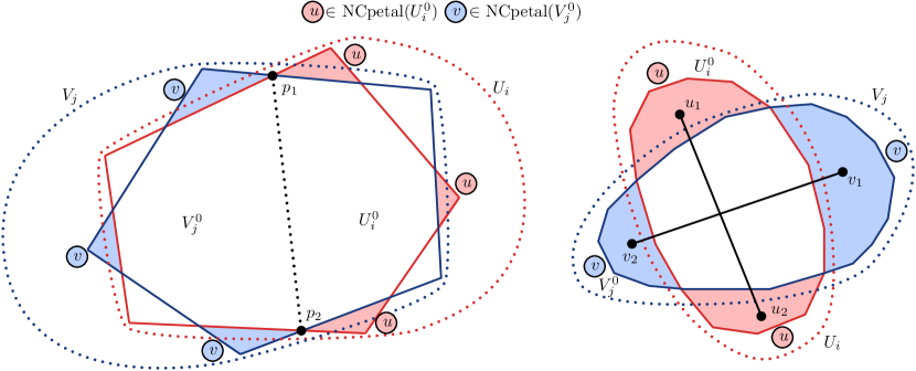
Figure 4: Illustration of Lemma 4.

∎

4 Dominating-Set for Homothetic Convex Objects

Let $\displaystyle C$ be a convex object in the plane. We fix an arbitrary interior point of $\displaystyle C$ as the center $\displaystyle c(C)$. We are given a set $\displaystyle\mathscr{S}$ of $\displaystyle n$ homothetic (i.e., translated and uniformly scaled) copies of $\displaystyle C$, and our objective is to show that the local-search algorithm given in Section 2 produces a PTAS for the minimum dominating-set for $\displaystyle\mathscr{S}$. Recall that $\displaystyle{\cal A}$ is the set of objects returned by the local-search algorithm, and $\displaystyle{\cal O}$ is a minimum dominating-set. Without loss of generality, we assume that both Claim 1 and 2 are satisfied.

In this section, we show mainly the existence of a planar graph satisfying the locality condition mentioned in Lemma 1. Here is an overview of the proof. First, we find a disjoint sub-decomposition $\displaystyle\widetilde{\cal A}\cup\widetilde{\cal O}$ of $\displaystyle{\cal A}\cup{\cal O}$ (in Lemma 5). Next, we consider a nearest-site Voronoi diagram for the sites in $\displaystyle\widetilde{\cal A}\cup\widetilde{\cal O}$ with respect to a distance function. Then we show (in Lemma 9) that the dual of this Voronoi diagram satisfies the locality condition mentioned in Lemma 1.

4.1 Decomposing into Interior Disjoint Convex Sites

Using Lemmas 3 and 4 as tools, now we prove the following which is one of the important observations of our work.

Lemma 5.

Let $\displaystyle{\cal A}$ be the output of the local-search algorithm for dominating-set on a set $\displaystyle\mathscr{S}$ of homothetic convex objects, and let $\displaystyle{\cal O}$ be the optimum dominating-set. Then there exists a disjoint sub-decomposition $\displaystyle\widetilde{\cal A}\cup\widetilde{\cal O}$ which satisfies the following: for any input object $\displaystyle S\in\mathscr{S}$ either

1. there exist $\displaystyle\widetilde{A}\in\widetilde{\cal A}$ and $\displaystyle\widetilde{O}\in\widetilde{\cal O}$ such that $\displaystyle S\cap\widetilde{A}\neq\emptyset$ and $\displaystyle S\cap\widetilde{O}\neq\emptyset$, or

2. there exist $\displaystyle{A}\in{\cal A}$ and $\displaystyle{O}\in{\cal O}$ such that $\displaystyle S\cap{A}\cap{O}\neq\emptyset$, and their traces $\displaystyle\widetilde{A}$ and $\displaystyle\widetilde{O}$ share an edge on their boundary.

Remainder of this section is devoted to the proof of this lemma. As a continuation from Section 2.1, we would like to remind the reader that duplicate objects have been pruned from $\displaystyle{\cal A}$ and $\displaystyle{\cal O}$.

Let $\displaystyle{\cal A}=\{A_{1},\ldots,A_{\ell}\}$ and $\displaystyle{\cal O}=\{O_{1},\ldots,O_{t}\}$. Our algorithm to obtain a disjoint sub-decomposition $\displaystyle\widetilde{\cal A}\cup\widetilde{\cal O}=\{\widetilde{A}_{1},\ldots\widetilde{A}_{\ell}\}\cup\{\widetilde{O}_{1},\ldots\widetilde{O}_{t}\}$ for $\displaystyle{\cal A}\cup{\cal O}$ satisfying the lemma statement is as follows.

Step 1: Obtaining decompositions individually: Note that the objects in $\displaystyle{\cal A}$ (resp., $\displaystyle{\cal O}$) are cover-free (follows from Claim 1). So, we apply Lemma 3 on the set $\displaystyle{\cal A}$ (resp., $\displaystyle{\cal O}$) of objects, to compute the disjoint decomposition of $\displaystyle{\cal A}$ (resp., $\displaystyle{\cal{O}}$). Let $\displaystyle{\cal A}^{0}=\{A^{0}_{1},\ldots,A^{0}_{\ell}\}$ (resp., $\displaystyle{\cal O}^{0}=\{O_{1}^{0},\ldots,O_{t}^{0}\}$ ) be the disjoint decomposition of $\displaystyle{\cal A}$ (resp., $\displaystyle{\cal{O}}$). Now, following claim is obvious.

Claim 4.

Any point $\displaystyle p\in\mathbb{R}^{2}$ is contained in the interior of at most two objects of $\displaystyle{\cal A}^{0}\cup{\cal O}^{0}$.

Lemma 3 ensures that $\displaystyle\operatorname{CF}({A_{i}},{\cal A})\subseteq A^{0}_{i}\neq\emptyset$ and $\displaystyle\operatorname{CF}({O_{j}},{\cal O})\subseteq O^{0}_{j}\neq\emptyset$ for all $\displaystyle i\in[\ell]$, $\displaystyle j\in[t]$. By Claim 2, no object $\displaystyle A^{0}_{i}$ can be properly contained in any single object from $\displaystyle{\cal O}^{0}$, but it may be completely covered by the union of two or more objects from $\displaystyle{\cal O}^{0}$. We can remedy this as follows.

Replace each object of $\displaystyle{\cal A}^{0}$ and $\displaystyle{\cal O}^{0}$ with an infinitesimally shrunken version of itself. By our assumption of general position, the resulting sets of shrunken objects still form dominating-sets. Furthermore, because the elements of $\displaystyle{\cal O}^{0}$ have pairwise disjoint interiors, no single object of $\displaystyle{\cal A}^{0}$ can be contained in the union of two or more of the shrunken objects in $\displaystyle{\cal O}^{0}$. Henceforth, $\displaystyle{\cal A}^{0}$ and $\displaystyle{\cal O}^{0}$ refer to the sets of shrunken objects. Thus we have the following.

Claim 5.

• $\displaystyle\operatorname{CF}(A^{0}_{i},{\cal A}^{0}\cup{\cal O}^{0})\neq\emptyset$ for all $\displaystyle i\in[\ell]$,

• $\displaystyle\operatorname{CF}(O^{0}_{j},{\cal A}^{0}\cup{\cal O}^{0})\neq\emptyset$ for all $\displaystyle j\in[t]$,

• For each object $\displaystyle S\in{\cal S}$, there exist an object $\displaystyle A_{i}^{0}\in{\cal A}^{0}$ (resp., $\displaystyle O_{j}^{0}\in{\cal O}^{0}$) such that $\displaystyle S\cap A_{i}^{0}\neq\emptyset$ (resp., $\displaystyle S\cap O_{j}^{0}\neq\emptyset$).

Step 2: Obtaining disjoint sub-decomposition: Now, consider $\displaystyle A^{0}_{i}\in{\cal A}^{0}$ for all $\displaystyle i\in[\ell]$. Lemma 3 ensures that $\displaystyle A^{0}_{i}$ does not have any interior overlap with $\displaystyle A^{0}_{k}$, for any $\displaystyle k\in[\ell]\setminus i$. Similarly, $\displaystyle{O^{0}_{j}}$ ($\displaystyle j\in[t]$) does not have any interior overlap with $\displaystyle O_{k}^{0}$, for any $\displaystyle k\in[t]\setminus j$. But, $\displaystyle A^{0}_{i}$ may have interior overlap with one or more objects of $\displaystyle{\cal O}^{0}$. Let $\displaystyle L(i)$ be the subset of indices $\displaystyle j\in[t]$ such that $\displaystyle A_{i}^{0}$ has an interior overlap with $\displaystyle O_{j}^{0}$. For any $\displaystyle j\in L(i)$, Claim 5 implies that both $\displaystyle\operatorname{CF}(A^{0}_{i},{\cal A}^{0}\cup{\cal O}^{0})\neq\emptyset$ and $\displaystyle\operatorname{CF}(O^{0}_{j},{\cal A}^{0}\cup{\cal O}^{0})\neq\emptyset$. By applying Lemma 4 to $\displaystyle A^{0}_{i}$ and $\displaystyle{O^{0}_{j}}$, we obtain two interior-disjoint convex objects $\displaystyle A_{ij}^{0}\subseteq A_{i}^{0}$ and $\displaystyle O_{ji}^{0}\subseteq O_{j}^{0}$. Let $\displaystyle A^{1}_{i}=\bigcap_{j\in L(i)}A_{ij}^{0}$. Similarly, let $\displaystyle M(j)$ be the subset of indices $\displaystyle i\in[l]$ such that $\displaystyle O_{j}^{0}$ has an interior overlap with $\displaystyle A_{i}^{0}$. Let $\displaystyle O^{1}_{j}=\bigcap_{i\in M(j)}O^{0}_{ji}$ which is a convex object and it contains $\displaystyle\operatorname{CF}(O_{j})$. Let $\displaystyle{\cal A}^{1}=\{A^{1}_{1},\ldots,A^{1}_{\ell}\}$ and $\displaystyle{\cal O}^{1}=\{{O^{1}_{1}},\ldots,{O^{1}_{t}}\}$. Clearly, $\displaystyle A_{i}^{1}\subseteq A_{i}^{0}$ and $\displaystyle O_{j}^{1}\subseteq O_{j}^{0}$, and since separating line segments $\displaystyle E_{ij}^{0}$ have eliminated all overlaps between the two decompositions, it follows that $\displaystyle{\cal A}^{1}\cup{\cal O}^{1}$ is a disjoint sub-decomposition of $\displaystyle{\cal A}\cup{\cal O}$. If we concentrate on the arrangements of all $\displaystyle E^{0}_{ij}$ along the boundary of $\displaystyle\partial A^{0}_{i}$, then we observe the following.

Claim 6.

Any two separating line segments $\displaystyle E^{0}_{ij}$ and $\displaystyle E^{0}_{ij^{\prime}}$ do not intersect each other.

Proof.

If $\displaystyle E^{0}_{ij}$ and $\displaystyle E^{0}_{ij^{\prime}}$ intersect each other then assertions (ii) and (iii) of Lemma 4 imply that the corresponding objects $\displaystyle{O^{0}_{j}}$ and $\displaystyle O_{j^{\prime}}^{0}$ also intersect, which is not possible because $\displaystyle{\cal O}^{0}$ is a disjoint decomposition. ∎

The boundary $\displaystyle\partial A^{1}_{i}$ is actually obtained by replacing zero or more disjoint arcs of $\displaystyle\partial A^{0}_{i}$ with separating line segments. Since each of these separating line segments are part of different disjoint objects in $\displaystyle{\cal O}^{0}$, here we would like to remark that the object $\displaystyle A^{1}_{i}$ is nonempty. For the similar reason, each object $\displaystyle O^{1}_{j}\in{\cal O}^{1}$ is nonempty. We denote the partial boundary $\displaystyle\Delta{A^{0}_{ij}}$ (resp., $\displaystyle\Delta{O^{0}_{ji}}$ ) by the portion of the boundary $\displaystyle\partial A^{0}_{i}$ (resp., $\displaystyle\partial{O^{0}_{j}}$) which is replaced by the edge $\displaystyle E^{0}_{ij}$ (see Figure 5(b) where partial boundary is marked as dotted).

Note the following.

Claim 7.

Let $\displaystyle A^{0}_{i}$ and $\displaystyle O^{0}_{j}$ be any two objects from $\displaystyle{\cal A}^{0}$ and $\displaystyle{\cal O}^{0}$, respectively, such that $\displaystyle\operatorname{int}({{A}^{0}_{i}})\cap\operatorname{int}({{O}^{0}_{j}})\neq\emptyset$ and $\displaystyle E^{0}_{ij}$ is not a part of $\displaystyle\partial A^{1}_{i}$. Then following properties must be satisfied:

• there exists an object $\displaystyle O^{0}_{j^{\prime}}$ in $\displaystyle{\cal O}^{0}$ such that $\displaystyle\operatorname{int}({{A}^{0}_{i}})\cap\operatorname{int}({{O}^{0}_{j^{\prime}}})\neq\emptyset$, $\displaystyle E^{0}_{i{j^{\prime}}}$ is a part of $\displaystyle\partial A^{1}_{i}$, and $\displaystyle{A}^{0}_{i}\setminus{A}^{0}_{ij}$ is completely contained in $\displaystyle{O}_{j^{\prime}}$.

• $\displaystyle O^{0}_{j}$ does not intersect $\displaystyle A^{1}_{i}$.

Proof.

Claim 6 implies that that no two separating line segments intersect each other, so the fact that $\displaystyle E^{0}_{ij}$ does not contribute to $\displaystyle\partial A^{1}_{i}$ implies that there is another object $\displaystyle{O^{0}_{j^{\prime}}}$ such that the partial-boundary $\displaystyle\Delta{A^{0}_{ij^{\prime}}}$ contains the partial boundary $\displaystyle\Delta{A^{0}_{ij}}$. Thus, $\displaystyle A^{0}_{ij^{\prime}}\subseteq A^{0}_{ij}$ which implies $\displaystyle{A}^{0}_{i}\setminus A^{0}_{ij}\subseteq{A}^{0}_{i}\setminus A^{0}_{ij^{\prime}}$. Since $\displaystyle{A}^{0}_{i}\setminus A^{0}_{ij^{\prime}}$ is completely contained in $\displaystyle{O}_{j^{\prime}}$ (by Lemma 4), $\displaystyle{A}^{0}_{i}\setminus A^{0}_{ij}$ is also completely contained in $\displaystyle{O}_{j^{\prime}}$.

Since $\displaystyle{O^{0}_{j}}$ and $\displaystyle{O^{0}_{j^{\prime}}}$ are interior disjoint and the partial-boundary $\displaystyle\Delta{A^{0}_{ij^{\prime}}}$ contains the partial boundary $\displaystyle\Delta{A^{0}_{ij}}$, $\displaystyle{O^{0}_{j}}$ cannot intersect $\displaystyle{A^{1}_{i}}$. Hence, the claim follows. ∎

By a symmetrical argument, we have the following.

Claim 8.

Let $\displaystyle A^{0}_{i}$ and $\displaystyle O^{0}_{j}$ be any two objects from $\displaystyle{\cal A}^{0}$ and $\displaystyle{\cal O}^{0}$, respectively, such that $\displaystyle\operatorname{int}({{A}^{0}_{i}})\cap\operatorname{int}({{O}^{0}_{j}})\neq\emptyset$ and $\displaystyle E^{0}_{ji}$ is not a part of $\displaystyle\partial O^{1}_{j}$. Then following properties must be satisfied:

• there exists an object $\displaystyle A^{0}_{i^{\prime}}$ in $\displaystyle{\cal A}^{0}$ such that $\displaystyle\operatorname{int}({{O}^{0}_{j}})\cap\operatorname{int}({{A}^{0}_{i^{\prime}}})\neq\emptyset$, $\displaystyle E^{0}_{j{i^{\prime}}}$ is a part of $\displaystyle\partial O^{1}_{j}$, and $\displaystyle{O}^{0}_{j}\setminus{O}^{0}_{ji}$ is completely contained in $\displaystyle{A}_{i^{\prime}}$.

• $\displaystyle A^{0}_{i}$ does not intersect $\displaystyle O^{1}_{j}$.

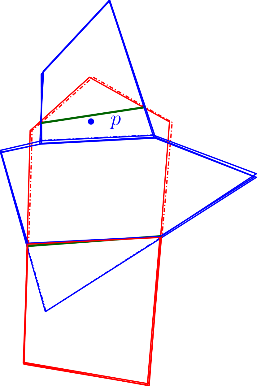
(a) After Step 1

(b) After Step 2 (Partial boundaries are shown dotted and the separating line segments are marked in green)

(c) After Step 3

Figure 5: Illustration of different steps: objects in $\displaystyle\cal A$ and $\displaystyle\cal O$ are marked with red and blue, respectively.

Note that after this step, there might be some point $\displaystyle p\in{{A}^{0}_{i}}$ but $\displaystyle p\notin{{A}^{1}_{i}}$ and there does not exist any $\displaystyle{{O}^{1}_{j}}$ such that $\displaystyle p\in{{O}^{1}_{j}}$ (see Figure 5(a-b)). Hence, the objects of $\displaystyle{\cal A}^{1}\cup{\cal O}^{1}$ fail to cover the same region as $\displaystyle{\cal A}^{0}\cup{\cal O}^{0}$, as needed in the decomposition. To remedy this, we expand some of the objects in $\displaystyle{\cal A}^{1}$ and $\displaystyle{\cal O}^{1}$ in the next step.

Step 3: Expansion of objects in $\displaystyle{\cal A}^{1}$ and $\displaystyle{\cal O}^{1}$:

For each $\displaystyle(i,j)\in[\ell]\times[t]$, define $\displaystyle\chi(i,j)=1$ if $\displaystyle E^{0}_{ij}$ is a part of $\displaystyle\partial A^{1}_{i}$ and $\displaystyle E^{0}_{ji}$ is also a part of $\displaystyle\partial O^{1}_{j}$, and it is $\displaystyle 0$ otherwise. Recalling $\displaystyle A^{0}_{ij}$ and $\displaystyle O^{0}_{ji}$ from Lemma 4, for each $\displaystyle i\in[\ell]$, define $\displaystyle A^{2}_{i}=\bigcap\limits_{\{j|\chi(i,j)=1\}}A^{0}_{ij}$, and for each $\displaystyle j\in[t]$, define $\displaystyle O^{2}_{j}=\bigcap\limits_{\{i|\chi(i,j)=1\}}O^{0}_{ji}$. Let $\displaystyle{\cal A}^{2}=\{A^{2}_{1},\ldots,A^{2}_{\ell}\}$ and $\displaystyle{\cal O}^{2}=\{{O^{2}_{1}},\ldots,{O^{2}_{t}}\}$. Note that $\displaystyle{\cal A}^{2}\cup{\cal O}^{2}$ is a disjoint sub-decomposition of $\displaystyle{\cal A}\cup{\cal O}$. This construction along with Claims 7 and 8 ensures the following.

Claim 9.

• For any point $\displaystyle p\in A^{0}_{i}\setminus A^{2}_{i}$, there exists some $\displaystyle{O^{2}_{j}}\in{\cal O}^{2}$ such that $\displaystyle{A^{2}_{i}}$ and $\displaystyle{O^{2}_{j}}$ share an edge on their boundary and $\displaystyle p\in O_{j}$.

• For any point $\displaystyle p\in O^{0}_{j}\setminus O^{2}_{j}$, there exists some $\displaystyle{A^{2}_{i}}\in{\cal A}^{2}$ such that $\displaystyle{A^{2}_{i}}$ and $\displaystyle{O^{2}_{j}}$ share an edge on their boundary and $\displaystyle p\in A_{i}$.

By renaming each set $\displaystyle A^{2}_{i}$ as $\displaystyle\widetilde{A}_{i}$ for $\displaystyle i\in[\ell]$ and each $\displaystyle O_{j}^{2}$ as $\displaystyle\widetilde{O}_{j}$ for $\displaystyle j\in[t]$, we obtain the final decomposition $\displaystyle\widetilde{\cal A}\cup\widetilde{\cal O}={\cal A}^{2}\cup{\cal O}^{2}$. Finally, we claim the following which completes the proof of the lemma statement.

Claim 10.

For any input object $\displaystyle S\in\mathscr{S}$ either (i) there exist $\displaystyle\widetilde{A}\in\widetilde{\cal A}$ and $\displaystyle\widetilde{O}\in\widetilde{\cal O}$ such that $\displaystyle S\cap\widetilde{A}\neq\emptyset$ and $\displaystyle S\cap\widetilde{O}\neq\emptyset$, or (ii) there exist $\displaystyle{A}\in{\cal A}$ and $\displaystyle{O}\in{\cal O}$ such that $\displaystyle S\cap{A}\cap{O}\neq\emptyset$, and $\displaystyle\widetilde{A}$ and $\displaystyle\widetilde{O}$ share an edge on their boundary.

Proof.

Let $\displaystyle S$ be any input object in $\displaystyle\mathscr{S}$. From Claim 5 (iii), we know that there exist $\displaystyle A^{0}_{i}\in{\cal A}^{0}$ and $\displaystyle O^{0}_{j}\in{\cal O}^{0}$ such that $\displaystyle S\cap A^{0}_{i}\neq\emptyset$ and $\displaystyle S\cap O^{0}_{j}\neq\emptyset$ for some $\displaystyle i\in[\ell]$ and $\displaystyle j\in[t]$. If after Step 3, $\displaystyle S\cap{A^{2}_{i}}\neq\emptyset$ and $\displaystyle S\cap{O^{2}_{j}}\neq\emptyset$, then the claim follows. So without loss of generality assume that $\displaystyle S\cap{A^{2}_{i}}=\emptyset$. Consider any point $\displaystyle p\in S\cap A^{0}_{i}$. As $\displaystyle p\in A^{0}_{i}\setminus{A^{2}_{i}}$, there exist some $\displaystyle{O^{2}_{j}}\in{\cal O}^{2}$ such that $\displaystyle{A^{2}_{i}}$ and $\displaystyle{O^{2}_{j}}$ share an edge on their boundary and $\displaystyle p\in O_{j}$ (follows from Claim 9). Thus the claim follows. ∎

4.2 Nearest-site Voronoi diagram

Recalling the definition of the convex distance function $\displaystyle\delta_{C}$ from Definition 1, we define the distance $\displaystyle\delta_{C}(p,P)$ from a point $\displaystyle p$ to any object $\displaystyle P$ (which need not be convex and homothetic to $\displaystyle C$) as follows.

Definition 3.

Let $\displaystyle p$ be a point and $\displaystyle P$ be an object in a plane. The distance $\displaystyle\delta_{C}(p,P)$ from $\displaystyle p$ to $\displaystyle P$ is defined as $\displaystyle\delta_{C}(p,P)=\min\limits_{q\in P}\delta_{C}(p,q)$.

This distance function has the following properties.

Property 2.

• If $\displaystyle p$ is contained in the object $\displaystyle P$, then $\displaystyle\delta_{C}(p,P)=0$.

• If $\displaystyle\delta_{C}(p,P)>0$, then $\displaystyle p$ is outside the object $\displaystyle P$, and a translated copy of $\displaystyle C$ centered at $\displaystyle p$ with scaling factor $\displaystyle\delta_{C}(p,P)$ touches the object $\displaystyle P$.

Now, we define a nearest-site Voronoi diagram $\displaystyle\operatorname{NVD}_{C}$ for all the objects in $\displaystyle\widetilde{\cal A}\cup\widetilde{\cal O}$ with respect to the distance function $\displaystyle{\delta}_{C}$.

We define Voronoi cell of $\displaystyle{S}_{i}\in\widetilde{\cal A}\cup\widetilde{\cal O}$ as $\displaystyle\operatorname{Cell}({S}_{i})=\{p\in\mathbb{R}^{2}|{\delta}_{C}(p,{S}_{i})\leq{\delta}_{C}(p,{S}_{j})\textit{~{}for all }j\neq i\}$. The $\displaystyle\operatorname{NVD}_{C}$ is a partition on the plane imposed by the collection of cells of all the objects in $\displaystyle\widetilde{\cal A}\cup\widetilde{\cal O}$. A point $\displaystyle p$ is in $\displaystyle\operatorname{Cell}({S})$ for some object $\displaystyle{S}\in\widetilde{\cal A}\cup\widetilde{\cal O}$, implies that if we place a homothetic copy of $\displaystyle C$ centered at $\displaystyle p$ with a scaling factor $\displaystyle\delta_{C}(p,S)$, then $\displaystyle C$ touches $\displaystyle{S}$ and the interior of $\displaystyle C$ is empty. Now, we have the following two lemmas.

Lemma 6.

The cell of every object $\displaystyle{S}\in\widetilde{\cal A}\cup\widetilde{\cal O}$ is nonempty. Moreover, $\displaystyle{S}\subseteq\operatorname{Cell}({S})$.

Proof.

This follows from Property 2(i) and the fact that $\displaystyle\widetilde{\cal A}\cup\widetilde{\cal O}$ is a set of interior disjoint objects (from Lemma 5(a)). ∎

Lemma 7.

Each cell $\displaystyle\operatorname{Cell}({S})$ is simply connected.

Proof.

For every $\displaystyle S\in\widetilde{\cal A}\cup\widetilde{\cal O}$, let us define the function $\displaystyle\pi_{S}\colon\mathbb{R}^{2}\to S$, that maps any point to one of its closest points in $\displaystyle S$. (If $\displaystyle p\in S$, then $\displaystyle\pi_{S}(p)=p$.)

We first claim that for every point $\displaystyle p\in\operatorname{Cell}(S)$, the line segment $\displaystyle\overline{p\pi_{S}(p)}\subseteq\operatorname{Cell}(S)$. To see this, suppose to the contrary that there exists a point $\displaystyle q\in\overline{p\pi_{S}(p)}$ such that $\displaystyle q\in\operatorname{Cell}(S^{\prime})$ where $\displaystyle S(^{\prime}\neq S)\in\widetilde{\cal A}\cup\widetilde{\cal O}$. Then by basic properties of convex distance functions (Property 1), we have

$$\delta_{C}(p,S^{\prime})\leq\delta_{C}(p,\pi_{S^{\prime}}(q))\leq\delta_{C}(p,q)+\delta_{C}(q,\pi_{S^{\prime}}(q))<\delta_{C}(p,q)+\delta_{C}(q,\pi_{S}(p))=\delta_{C}(p,\pi_{S}(p)),$$

contradicting the fact that $\displaystyle p\in\operatorname{Cell}(S)$.

To see that $\displaystyle\operatorname{Cell}(S)$ is connected, observe that any two points $\displaystyle p,p^{\prime}\in\operatorname{Cell}(S)$ can be connected as follows. First, connect $\displaystyle p$ to $\displaystyle\pi_{S}(p)$ and $\displaystyle p^{\prime}$ to $\displaystyle\pi_{S}(p^{\prime})$. Then connect these two points through $\displaystyle S$. By the above claim and Lemma 6, all of these segments lies within $\displaystyle\operatorname{Cell}(S)$.

To complete the proof that $\displaystyle\operatorname{Cell}(S)$ is simply connected, we use the well known equivalent characterization [23] that for any simple closed (i.e., Jordan) curve $\displaystyle\Psi\subset\operatorname{Cell}(S)$, the interior of the region bounded by this curve lies entirely within $\displaystyle\operatorname{Cell}(S)$. Consider any $\displaystyle x$ in the interior of the region bounded by $\displaystyle\Psi$. Either $\displaystyle x\in S$ or (by extending the ray from $\displaystyle\pi_{S}(x)$ through $\displaystyle x$ until it hits $\displaystyle\Psi$) there exists $\displaystyle p\in\operatorname{Cell}(S)$ such that $\displaystyle x$ lies on the line segment $\displaystyle\overline{p\pi_{S}(x)}$. In the former case, $\displaystyle x\in\operatorname{Cell}(S)$, follows from Lemma 6. Now, we are going to argue that $\displaystyle x\in\operatorname{Cell}(S)$ for the latter case as well. To see this, suppose to the contrary that $\displaystyle x\in\operatorname{Cell}(S^{\prime})$ where $\displaystyle S(^{\prime}\neq S)\in\widetilde{\cal A}\cup\widetilde{\cal O}$. Then by basic properties of convex distance functions (Property 1), we have

$$\delta_{C}(p,S^{\prime})\leq\delta_{C}(p,\pi_{S^{\prime}}(x))\leq\delta_{C}(p,x)+\delta_{C}(x,\pi_{S^{\prime}}(q))<\delta_{C}(p,x)+\delta_{C}(x,\pi_{S}(p))=\delta_{C}(p,\pi_{S}(p)),$$

contradicting the fact that $\displaystyle p\in\operatorname{Cell}(S)$. Therefore $\displaystyle x\in\operatorname{Cell}(S)$, as desired. ∎

4.3 Locality Condition

Let us consider the graph $\displaystyle{\cal G}=({\cal V},{\cal E})$, the dual of the Voronoi diagram $\displaystyle\operatorname{NVD}_{C}$, whose vertices $\displaystyle\mathcal{V}$ are the elements of $\displaystyle\mathcal{A}\cup\mathcal{O}$ and the edge set $\displaystyle\mathcal{E}$ consists of pairs $\displaystyle U,V\in\mathcal{V}$ whose Voronoi cells share an edge on their boundaries. From Lemma 6 and Lemma 7, we have the following.

Lemma 8.

The graph $\displaystyle{\cal G}=({\cal A}\cup{\cal O},{\cal E})$ is a planar graph.

Now, we prove that the graph $\displaystyle{\cal G}$ satisfies the property needed in the locality condition (Lemma 1).

Lemma 9.

For any arbitrary input object $\displaystyle S\in\mathscr{S}$, if $\displaystyle S$ is dominated by at least one object of $\displaystyle\cal A$ and at least one object of $\displaystyle\cal O$, then there exists $\displaystyle A\in{\cal A}$ and $\displaystyle O\in{\cal O}$ both of which dominate $\displaystyle S$ and $\displaystyle(A,O)\in{\cal E}$ of $\displaystyle{\cal G}$.

Proof.

Let $\displaystyle S$ be any object in $\displaystyle\mathscr{S}$. According to Lemma 5, there exists a disjoint sub-decomposition $\displaystyle\widetilde{\cal A}\cup\widetilde{\cal O}$ such that either:

• there exist $\displaystyle\widetilde{A}\in\widetilde{\cal A}$ and $\displaystyle\widetilde{O}\in\widetilde{\cal O}$ such that $\displaystyle S\cap\widetilde{A}$ and $\displaystyle S\cap\widetilde{O}$ are both nonempty, or

• there exist $\displaystyle{A}\in{\cal A}$ and $\displaystyle{O}\in{\cal O}$ such that $\displaystyle S\cap{A}\cap{O}\neq\emptyset$, and their respective traces $\displaystyle\widetilde{A}$ and $\displaystyle\widetilde{O}$ share an edge in common on their boundaries.

For case (ii), clearly both $\displaystyle A$ and $\displaystyle O$ dominates $\displaystyle S$. The fact that $\displaystyle\widetilde{A}$ and $\displaystyle\widetilde{O}$ share a common edge on their boundary implies (by Lemma 6) that $\displaystyle\operatorname{Cell}(\widetilde{A})$ and $\displaystyle\operatorname{Cell}(\widetilde{O})$ also share a common edge on their boundaries. Therefore, $\displaystyle(A,O)$ is an edge of $\displaystyle\mathcal{G}$, as desired.

For case (i), let $\displaystyle c=c(S)$ denote the center of $\displaystyle S$. Without loss of generality, we may assume that $\displaystyle A$ and $\displaystyle O$ have been chosen so that $\displaystyle\widetilde{A}$ and $\displaystyle\widetilde{O}$ are the closest objects to $\displaystyle c$ (with respect to $\displaystyle\delta_{C}$) in $\displaystyle\widetilde{\mathcal{A}}$ and $\displaystyle\widetilde{\mathcal{O}}$, respectively. We may assume that $\displaystyle\delta_{C}(c,\widetilde{A})\leq\delta_{C}(c,\widetilde{O})$ (as the other case is symmetrical).

Let $\displaystyle o\in\widetilde{O}$ denote the closest point to $\displaystyle c$ in $\displaystyle\widetilde{O}$. Clearly, $\displaystyle c$ and $\displaystyle o$ lie in different Voronoi cells, so this segment must intersect an edge of $\displaystyle\operatorname{Cell}(\widetilde{O})$ at some point $\displaystyle p$. Let $\displaystyle\operatorname{Cell}(\widetilde{R})$ denote the cell neighbouring the $\displaystyle\operatorname{Cell}(\widetilde{O})$ along this edge. Letting $\displaystyle r$ denote the closest point to $\displaystyle p$ in $\displaystyle\widetilde{R}$, we have $\displaystyle\delta_{C}(p,r)=\delta_{C}(p,\widetilde{R})=\delta_{C}(p,\widetilde{O})\leq\delta_{C}(p,o)$. By basic properties of convex distance function (see Property 1) we obtain

$$\delta_{C}(c,r)\leq\delta_{C}(c,p)+\delta_{C}(p,r)\leq\delta_{C}(c,p)+\delta_{C}(p,o)=\delta_{C}(c,o).$$

By general position, we may assume that $\displaystyle\delta_{C}(c,\widetilde{R})<\delta_{C}(c,\widetilde{O})$. Since $\displaystyle\widetilde{O}$ was chosen to be the closest object in $\displaystyle\widetilde{O}$ to $\displaystyle c$, it follows that $\displaystyle\widetilde{R}\in\widetilde{\mathcal{A}}$. Clearly, the associated objects $\displaystyle R$ and $\displaystyle O$ (which contain $\displaystyle\widetilde{R}$ and $\displaystyle\widetilde{O}$, respectively) both dominates $\displaystyle S$. Therefore, there is an edge $\displaystyle(R,O)$ in $\displaystyle\mathcal{G}$, as desired. ∎

5 Dominating-Set for Homothets of a Centrally Symmetric Convex Object

In this section, we give a simpler analysis of the local search algorithm for the dominating-set problem when the objects are homothets of a centrally symmetric convex object. Our analysis is a generalization of Gibson et al. [16] where we can avoid the sophisticated tool of disjoint decomposition.

Let $\displaystyle C$ be a centrally symmetric convex object in the plane with the center $\displaystyle c(C)$. Given a set $\displaystyle\mathscr{S}$ of homothets of $\displaystyle C$, our objective is to show that the local-search algorithm given in Section 2 is a PTAS for the minimum dominating-set for $\displaystyle\mathscr{S}$. Recall that $\displaystyle{\cal A}$ is the set of objects returned by the local-search algorithm, and $\displaystyle{\cal O}$ is the minimum dominating-set. As a continuation from Section 2, we assume that both Claim 1 and 2 are satisfied.

As in Section 4.2, we define a nearest-site Voronoi diagram for all objects in $\displaystyle{\cal A}\cup{\cal O}$ with respect to a distance function $\displaystyle\delta_{C}^{*}$. First, we are going to extend the convex distance function to provide meaningful (albeit negative) to the interior of each site. This would allow us to interpret the Voronoi diagram as a Voronoi diagram of additively weighted points, rather than a Voronoi diagram of (unweighted) regions. For each object $\displaystyle S\in\mathscr{S}$, we define the weight $\displaystyle w(S)$ to be $\displaystyle\alpha$, where $\displaystyle S=c(S)+\alpha C$. Now, we define the distance $\displaystyle\delta_{C}^{*}(p,S)$ between a point $\displaystyle p\in\mathbb{R}^{2}$ and an object $\displaystyle S\in\mathscr{S}$ as follows: $\displaystyle\delta_{C}^{*}(p,S)=\delta_{C}(p,c({S}))-w(S)$. The distance function $\displaystyle\delta_{C}^{*}(p,S)$ has the following properties:

Property 3.

1. The distance function $\displaystyle\delta_{C}^{*}(p,S)$ achieves its minimum value when $\displaystyle p=c(S)$.

2. If $\displaystyle p$ is contained in the object $\displaystyle S$, then $\displaystyle\delta_{C}^{*}(p,S)\leq 0$.

3. If $\displaystyle\delta_{C}^{*}(p,S)>0$, then $\displaystyle p$ is outside the object $\displaystyle S$, and a translated copy of $\displaystyle C$ centered at $\displaystyle p$ with scaling factor $\displaystyle\delta_{C}^{*}(p,S)$ touches the object $\displaystyle S$.

Note that Property 3(iii) is crucial for our analysis and it follows due to the symmetric property of $\displaystyle\delta_{C}$. As a result, this approach cannot be applied when objects are not centrally symmetric.

We will show that each object in $\displaystyle{\cal A}\cup{\cal O}$ has a nonempty cell in this Voronoi diagram and each cell is simply connected. As a result the graph $\displaystyle{\cal G}=({\cal V},{\cal E})$ which is the dual of this Voronoi diagram is planar. Finally, we will show that this graph satisfies the locality condition mentioned in Lemma 1. This completes the proof.

Lemma 10.

The cell of every object $\displaystyle{S}\in{\cal A}\cup{\cal O}$ is nonempty. Moreover, the center $\displaystyle c({S})\subseteq\operatorname{Cell}({S})$.

Proof.

For the sake of contradiction, assume for some object $\displaystyle S\in{\cal A}\cup{\cal O}$, $\displaystyle c(S)\notin\operatorname{Cell}(S)$ and $\displaystyle c(S)\in\operatorname{Cell}(S^{\prime})$ where $\displaystyle S^{\prime}(\neq S)\in{\cal A}\cup{\cal O}$. So, $\displaystyle\delta_{C}^{*}(c(S),S)\geq\delta_{C}^{*}(c(S),S^{\prime})$. Since $\displaystyle\delta_{C}^{*}(c(S),S)=-w(S)$, we have $\displaystyle-w(S)\geq\delta_{C}(c(S),c(S^{\prime}))-w(S^{\prime})$. This implies $\displaystyle w(S^{\prime})\geq\delta_{C}(c(S),c(S^{\prime}))+w(S)$ which means that the object $\displaystyle S$ is contained in the object $\displaystyle S^{\prime}$. This contradicts Claim 1 and 2. ∎

Lemma 11.

Each cell $\displaystyle\operatorname{Cell}({S})$ is simply connected.

Proof.

We first claim that for every point $\displaystyle p\in\operatorname{Cell}(S)$, the line segment $\displaystyle\overline{pc(S)}\subseteq\operatorname{Cell}(S)$. To see this, suppose to the contrary that there exists a point $\displaystyle q\in\overline{pc(S)}$ such that $\displaystyle q\in\operatorname{Cell}(S^{\prime})$ where $\displaystyle S^{\prime}(\neq S)\in{\cal A}\cup{\cal O}$. Then by basic properties of convex distance functions (Property 1), we have

$$\delta_{C}^{*}(p,S^{\prime})=\delta_{C}(p,c(S^{\prime}))-w(S^{\prime})\leq\delta_{C}(p,q)+\delta_{C}(q,c(S^{\prime}))-w(S^{\prime})\leq\delta_{C}(p,q)+\delta_{C}^{*}(q,S^{\prime})$$

$$<\delta_{C}(p,q)+\delta_{C}^{*}(q,S)=\delta_{C}(p,q)+\delta_{C}(q,c(S))-w(S)=\delta_{C}(p,c(S))-w(S)=\delta_{C}^{*}(p,S),$$

contradicting the fact that $\displaystyle p\in\operatorname{Cell}(S)$.

To see that $\displaystyle\operatorname{Cell}(S)$ is connected, observe that any two points $\displaystyle p,p^{\prime}\in\operatorname{Cell}(S)$ can be connected via $\displaystyle c(S)$ as follows. First, connect $\displaystyle p$ to $\displaystyle c(S)$ and then connect $\displaystyle p^{\prime}$ to $\displaystyle c(S)$. By the above claim and Lemma 10, all of these segments lies within $\displaystyle\operatorname{Cell}(S)$.

To complete the proof that $\displaystyle\operatorname{Cell}(S)$ is simply connected, we use the well known equivalent characterization [23] that for any simple closed (i.e., Jordan) curve $\displaystyle\Psi\subset\operatorname{Cell}(S)$, the interior of the region bounded by this curve lies entirely within $\displaystyle\operatorname{Cell}(S)$. Consider any $\displaystyle x$ in the interior of the region bounded by $\displaystyle\Psi$. Either $\displaystyle x=c(S)$ or (by extending the ray from $\displaystyle c(S)$ through $\displaystyle x$ until it hits $\displaystyle\Psi$) there exists $\displaystyle p\in\operatorname{Cell}(S)$ such that $\displaystyle x$ lies on the line segment $\displaystyle\overline{pc(S)}$. In the former case, $\displaystyle x\in\operatorname{Cell}(S)$, follows from Lemma 10. For the latter case, by the above claim (that $\displaystyle\overline{pc(S)}\subseteq\operatorname{Cell}(S)$), we have $\displaystyle x\in\operatorname{Cell}(S)$. This completes the proof. ∎

Lemma 12.

For any arbitrary input object $\displaystyle S\in\mathscr{S}$, there is an edge between $\displaystyle(A,O)\in{\cal G}$ such that $\displaystyle A\in{\cal A}$ and $\displaystyle O\in{\cal O}$, and both $\displaystyle A$ and $\displaystyle O$ dominates $\displaystyle S$.

Proof.

The proof is similar to the Case (i) of Lemma 9. ∎

6 Geometric Set-Cover for Convex Pseudodisks

Given a set $\displaystyle\mathscr{S}$ of $\displaystyle n$ convex pseudodisks and a set $\displaystyle\cal P$ of points in $\displaystyle\mathbb{R}^{2}$, the objective is to cover all the points in $\displaystyle\cal P$ using subset of $\displaystyle\mathscr{S}$ of minimum cardinality. Here, we analyze that the local search algorithm, as given in Section 2, would give a polynomial time approximation scheme. The analysis is similar to the previous problem. Recall from Section 2.1 that $\displaystyle{\cal O}$ is an optimal covering set for $\displaystyle\cal P$ and $\displaystyle{\cal A}$ is the covering set returned by our local search algorithm satisfying both Claim 1 and 2. Here, we need to show that the locality condition mentioned in Lemma 2 is satisfied.

If we restrict the proof of Lemma 5 up to Claim 9, then, it is straightforward to obtain the following.

Lemma 13.

Let $\displaystyle{\cal A}$ be the output of the local-search algorithm for set-cover on a set $\displaystyle\mathscr{S}$ of convex pseudodisks and a set $\displaystyle\cal P$ of points in $\displaystyle\mathbb{R}^{2}$, and let $\displaystyle{\cal O}$ be the optimum. Then there exists a disjoint sub-decomposition $\displaystyle\widetilde{\cal A}\cup\widetilde{\cal O}$ which satisfies the following: for any input point $\displaystyle p\in{\cal P}$ there exist $\displaystyle{A}\in{\cal A}$ and $\displaystyle{O}\in{\cal O}$ such that $\displaystyle p\in{A}$ and $\displaystyle p\in{O}$, and their traces $\displaystyle\widetilde{A}$ and $\displaystyle\widetilde{O}$ share an edge on their boundary.

Proof.

Let $\displaystyle{\cal A}=\{A_{1},\ldots,A_{\ell}\}$ and $\displaystyle{\cal O}=\{O_{1},\ldots,O_{t}\}$. Our algorithm to obtain a disjoint sub-decomposition $\displaystyle\widetilde{\cal A}\cup\widetilde{\cal O}=\{\widetilde{A}_{1},\ldots\widetilde{A}_{\ell}\}\cup\{\widetilde{O}_{1},\ldots\widetilde{O}_{t}\}$ for $\displaystyle{\cal A}\cup{\cal O}$ satisfying the lemma statement is exactly same as the three steps mentioned in Section 4.1 for Lemma 5. The main difference is in the statement of Claim 8. For set-cover problem, we have the following

Claim 11.

• $\displaystyle\operatorname{CF}(A^{0}_{i},{\cal A}^{0}\cup{\cal O}^{0})\neq\emptyset$ for all $\displaystyle i\in[\ell]$,

• $\displaystyle\operatorname{CF}(O^{0}_{j},{\cal A}^{0}\cup{\cal O}^{0})\neq\emptyset$ for all $\displaystyle j\in[t]$,

• Each point $\displaystyle p\in{\cal P}$ is covered by exactly one object from $\displaystyle{\cal A}^{0}$ (resp., $\displaystyle{\cal O}^{0}$).

Finally, instead of Claim 10, we claim the following statement.

Claim 12.

For any input point $\displaystyle p\in{\cal P}$, there exist $\displaystyle{A}\in{\cal A}$ and $\displaystyle{O}\in{\cal O}$ such that $\displaystyle p\in{A}$ and $\displaystyle p\in{O}$, and $\displaystyle\widetilde{A}$ and $\displaystyle\widetilde{O}$ share an edge on their boundary.

Proof.

Let $\displaystyle p$ be any input point in $\displaystyle{\cal P}$. By Claim 11 (iii), there exist $\displaystyle A^{0}_{i}\in{\cal A}^{0}$ and $\displaystyle O^{0}_{j}\in{\cal O}^{0}$ such that $\displaystyle p\in A^{0}_{i}$ and $\displaystyle p\in O^{0}_{j}$ for some $\displaystyle i\in[\ell]$ and $\displaystyle j\in[t]$. After Step 3, since $\displaystyle{\cal A}^{2}\cup{\cal O}^{2}$ is a disjoint decomposition of $\displaystyle{\cal A}\cup{\cal O}$, $\displaystyle p$ cannot be both in $\displaystyle{A^{2}_{i}}$ and $\displaystyle{O^{2}_{j}}$. Therefore, either of the following happens: $\displaystyle p\notin{A^{2}_{i}}$, or $\displaystyle p\notin{O^{2}_{j}}$. In both cases, the claim follows from Claim 9. ∎

Thus the lemma follows. ∎

Now, consider a graph $\displaystyle{\cal G}=({\cal V},{\cal E})$, where each vertex $\displaystyle V\in{\cal V}$ corresponds to an object in $\displaystyle\widetilde{\cal A}\cup\widetilde{\cal O}$, and we create an edge in between two vertices whenever the corresponding objects in $\displaystyle\widetilde{\cal A}\cup\widetilde{\cal O}$ share an edge in their boundary. Since, the objects of $\displaystyle\widetilde{\cal A}\cup\widetilde{\cal O}$ are convex and have disjoint interiors, this graph is a planar graph. From Lemma 13, it follows that the graph $\displaystyle{\cal G}$ satisfies the locality condition mentioned in Lemma 2. This completes the proof of Theorem 2.

7 Concluding Remarks

In this paper, we have shown that the well-known local search algorithm gives a PTAS for finding the minimum cardinality dominating-set and geometric set-cover when the objects are homothetic convex objects, and convex pseudodisks, respectively. As a consequence, we obtain easy to implement approximation guaranteed algorithms for a broad class of objects which encompasses arbitrary squares, $\displaystyle k$-regular polygons, translates of convex polygons. A QPTAS is known for the weighted set-cover problem where objects are pseudodisks [28]. But, no QPTAS is known for the weighted dominating-set problem when objects are homothetic convex objects. Note that the separator-based arguments for finding PTAS has a limitation for handling the weighted version of the problems. Thus, finding a polynomial time approximation scheme for the weighted version of both minimum dominating-set and minimum geometric set-cover problems for homothetic convex objects, pseudodisks remain open in this context. Specially, for the weighted version of the problem, it would be interesting to analyze the approximation guarantees of local search algorithm.

References

- [1] Anna Adamaszek and Andreas Wiese. A QPTAS for maximum weight independent set of polygons with polylogarithmically many vertices. In Proceedings of the Twenty-Fifth Annual ACM-SIAM Symposium on Discrete Algorithms, SODA 2014, Portland, Oregon, USA, January 5-7, 2014, pages 645–656, 2014.
- [2] Nikhil Bansal and Kirk Pruhs. The geometry of scheduling. SIAM J. Comput., 43(5):1684–1698, 2014.
- [3] Timothy M. Chan and Elyot Grant. Exact algorithms and APX-hardness results for geometric packing and covering problems. Comput. Geom., 47(2):112–124, 2014.
- [4] Timothy M. Chan and Sariel Har-Peled. Approximation algorithms for maximum independent set of pseudo-disks. In Proceedings of the 25th ACM Symposium on Computational Geometry, Aarhus, Denmark, June 8-10, 2009, pages 333–340, 2009.
- [5] Chandra Chekuri, Kenneth L. Clarkson, and Sariel Har-Peled. On the set multicover problem in geometric settings. ACM Transactions on Algorithms, 9(1):9, 2012.
- [6] L. Paul Chew and Robert L. (Scot) Drysdale III. Voronoi diagrams based on convex distance functions. In Proceedings of the First Annual Symposium on Computational Geometry, Baltimore, Maryland, USA, June 5-7, 1985, pages 235–244, 1985.
- [7] Kenneth L. Clarkson and Kasturi R. Varadarajan. Improved approximation algorithms for geometric set cover. Discrete & Computational Geometry, 37(1):43–58, 2007.
- [8] Vincent Cohen-Addad and Claire Mathieu. Effectiveness of local search for geometric optimization. In 31st International Symposium on Computational Geometry, SoCG 2015, June 22-25, 2015, Eindhoven, The Netherlands, pages 329–343, 2015.
- [9] Irit Dinur and David Steurer. Analytical approach to parallel repetition. In Symposium on Theory of Computing, STOC 2014, New York, NY, USA, May 31 - June 03, 2014, pages 624–633, 2014.
- [10] Herbert Edelsbrunner. The union of balls and its dual shape. Discrete & Computational Geometry, 13:415–440, 1995.
- [11] Thomas Erlebach and Erik Jan van Leeuwen. Domination in geometric intersection graphs. In LATIN 2008: Theoretical Informatics, 8th Latin American Symposium, Búzios, Brazil, April 7-11, 2008, Proceedings, pages 747–758, 2008.
- [12] Thomas Erlebach and Erik Jan van Leeuwen. PTAS for weighted set cover on unit squares. In Approximation, Randomization, and Combinatorial Optimization. Algorithms and Techniques, 13th International Workshop, APPROX 2010, and 14th International Workshop, RANDOM 2010, Barcelona, Spain, September 1-3, 2010. Proceedings, pages 166–177, 2010.
- [13] Uriel Feige. A threshold of ln n for approximating set cover. J. ACM, 45(4):634–652, 1998.
- [14] Greg N. Frederickson. Fast algorithms for shortest paths in planar graphs, with applications. SIAM J. Comput., 16(6):1004–1022, 1987.
- [15] M. R. Garey and David S. Johnson. Computers and Intractability: A Guide to the Theory of NP-Completeness. W. H. Freeman, 1979.
- [16] Matt Gibson and Imran A. Pirwani. Algorithms for dominating set in disk graphs: Breaking the logn barrier - (extended abstract). In Algorithms - ESA 2010, 18th Annual European Symposium, Liverpool, UK, September 6-8, 2010. Proceedings, Part I, pages 243–254, 2010.
- [17] Sariel Har-Peled and Mira Lee. Weighted geometric set cover problems revisited. JoCG, 3(1):65–85, 2012.
- [18] Sariel Har-Peled and Kent Quanrud. Approximation algorithms for polynomial-expansion and low-density graphs. In Algorithms - ESA 2015 - 23rd Annual European Symposium, Patras, Greece, September 14-16, 2015, Proceedings, pages 717–728, 2015.
- [19] Dorit S. Hochbaum and Wolfgang Maass. Fast approximation algorithms for a nonconvex covering problem. J. Algorithms, 8(3):305–323, 1987.
- [20] Viggo Kann. On the Approximability of NP-complete Optimization Problems. PhD thesis, Royal Institute of Technology, 1992.
- [21] Richard M Karp. Reducibility among combinatorial problems. In Complexity of Computer Computations, pages 85–103, 1972.
- [22] J.L. Kelley and I. Namioka. Linear Topological Spaces. Springer-Verlag, 1976.
- [23] Rolf Klein and Derick Wood. Voronoi diagrams based on general metrics in the plane. In STACS 88, 5th Annual Symposium on Theoretical Aspects of Computer Science, Bordeaux, France, February 11-13, 1988, Proceedings, pages 281–291, 1988.
- [24] Christoph Lenzen and Roger Wattenhofer. Minimum dominating set approximation in graphs of bounded arboricity. In Distributed Computing, 24th International Symposium, DISC 2010, Cambridge, MA, USA, September 13-15, 2010. Proceedings, pages 510–524, 2010.
- [25] Jian Li and Yifei Jin. A PTAS for the weighted unit disk cover problem. In Automata, Languages, and Programming - 42nd International Colloquium, ICALP 2015, Kyoto, Japan, July 6-10, 2015, Proceedings, Part I, pages 898–909, 2015.
- [26] Dániel Marx. Parameterized complexity of independence and domination on geometric graphs. In Parameterized and Exact Computation, Second International Workshop, IWPEC 2006, Zürich, Switzerland, September 13-15, 2006, Proceedings, pages 154–165, 2006.
- [27] Dániel Marx. Parameterized complexity and approximation algorithms. Comput. J., 51(1):60–78, 2008.
- [28] Nabil H. Mustafa, Rajiv Raman, and Saurabh Ray. Quasi-polynomial time approximation scheme for weighted geometric set cover on pseudodisks and halfspaces. SIAM J. Comput., 44(1):1650–1669, 2015.
- [29] Nabil H. Mustafa and Saurabh Ray. Improved results on geometric hitting set problems. Discrete & Computational Geometry, 44(4):883–895, 2010.
- [30] Ran Raz and Shmuel Safra. A sub-constant error-probability low-degree test, and a sub-constant error-probability PCP characterization of NP. In Proceedings of the Twenty-Ninth Annual ACM Symposium on the Theory of Computing, STOC 1997, El Paso, Texas, USA, May 4-6, 1997, pages 475–484, 1997.
- [31] Erik Jan van Leeuwen. Optimization and Approximation on Systems of Geometric Objects. PhD thesis, University of Amsterdam, 2009.
- [32] Kasturi R. Varadarajan. Weighted geometric set cover via quasi-uniform sampling. In Proceedings of the 42nd ACM Symposium on Theory of Computing, STOC 2010, Cambridge, Massachusetts, USA, 5-8 June 2010, pages 641–648, 2010.