Application of the QCD light cone sum rule to tetraquarks: the strong vertices $X_{b}X_{b}\rho$ and $X_{c}X_{c}\rho$

Abstract

The full version of QCD light-cone sum rule method is applied to tetraquarks containing a single heavy $b$ or $c$ quark. To this end, investigations of the strong vertices $X_{b}X_{b}\rho$ and $X_{c}X_{c}\rho$ are performed, where $X_{b}=[su][\bar{b}\bar{d}]$ and $X_{c}=[su][\bar{c}\bar{d}]$ are the exotic states built of four quarks of different flavors. The strong coupling constants $G_{X_{b}X_{b}\rho}$ and $G_{X_{c}X_{c}\rho}$ corresponding to these vertices are found using the $\rho$-meson leading and higher-twist distribution amplitudes. In the calculations $X_{b}$ and $X_{c}$ are treated as scalar bound states of a diquark and antidiquark.

I Introduction

During last decade, due to experimental data of the Belle, BaBar, LHCb, D0 and BES collaborations, which provided valuable information on the so-called exotic hadron states, this branch of high energy physics demonstrates a rapid growth. The exotic hadrons, i.e. ones that cannot be embraced by the spectroscopy of the known hadrons as $q\bar{q}$ or $qqq$ bound states, may serve as a laboratory for testing the Quantum Chromodynamics (QCD)- the existing theory of strong interactions, as well as various phenomenological models built of on its basis. An existence of the exotic hadrons does not contradict the fundamental principles of this theory. Though relevant problems attracted an interest of physicists from first years of the parton model and, later QCD, only recently these ideas found their experimental confirmation.

The discovery of the charmonium-like resonance $X(3872)$ by the Belle Collaboration Choi:2003ue was the first brick laid on footing of the house, which now exists as XYZ family of the exotic states. The observation made by the Belle was later reexamined and confirmed by other collaborations Abazov:2004kp ; Acosta:2003zx ; Aubert:2004ns . Produced in the $B$ meson decays or in the $pp$ collisions, observed in the $e^{+}e^{-}$ annihilation or in the two-photon fusion, exotic states remain on the focus of the main experimental collaborations, which collected wide data base on the processes of interest.

A considerable progress was made in the theoretical understanding of the features of the exotic states, as well. If experiments are devoted to measuring of the masses, and decay widths, to identifying the spins and parities of the exotic states, theoretical works are concentrated on studies of their internal quark-gluon structure, on new models and methods suggested for their exploration (for details of theoretical and experimental studies see, the reviews Jaffe:2004ph ; Swanson:2006st ; Klempt:2007cp ; Godfrey:2008nc ; Voloshin:2007dx ; Nielsen:2009uh ; Faccini:2012pj ; Esposito:2014rxa ; Chen:2016 , and references therein).

The charmonium-like resonances of the XYZ family contain, as it is evident from their names, a $c\bar{c}$ component. Therefore, efforts were done to explain the new resonances as excitations of the ordinary $c\overline{c}$ charmonium. Indeed, some of new particles allow such interpretation, and are really excited $c\overline{c}$ states. But the essential part of the relevant experimental data cannot be included into the exited charmonium scheme, and hence for their exploration unconventional quark-gluon configurations are needed. For this purpose, various models with different quark-gluon structures were supposed. The tetraquark model of the exotic states, i.e. the model that considers exotics as the four-quark particles, is among mostly employed ones. It is worth to note that this approach led to significant achievements in describing of the processes with the exotic states, in predicting their masses, decay widths and quantum numbers. There are some alternatives to compose from the four quarks an exotic state within the tetraquark model. In fact, the four constituent quarks may group into a diquark and an antidiquark to form the exotic state with required quantum numbers. This model is known as the diquark-antidiquark model. In the meson molecule picture the quarks are collected into two conventional mesons, and the exotic particle appears as loosely-bound molecule state. There are other opportunities to organize the exotic states from the four quarks, as well as alternative models, for an example, the hybrid models detailed presentation of which is beyond the scope of the present work.

In the tetraquark model the maximal number of the quark flavors in the XYZ states does not exceed three. But there are not any fundamental laws in QCD forbidding the existence of the exotic states built of four quarks of distinct flavors. Namely such exotic states recently became the objects of comprehensive theoretical investigations. But before going into details of these studies, we have to make some comments on the experimental situation formed around one of such particles. Strictly speaking, all present theoretical activity was inspired by the D0 collaboration’s report, where an evidence for existence of the exotic state $X(5568)$ was announced D0:2016mwd . Based on analysis of $p\bar{p}$ collision data at $\sqrt{s}=1.96\ \mathrm{TeV}$ collected at the Fermilab Tevatron collider, the collaboration reported on evidence of a narrow resonance $X(5568)$ in the consecutive decays $X(5568)\to B_{s}^{0}\pi^{\pm}$, $B_{s}^{0}\to J/\psi\phi$, $J/\psi\to\mu^{+}\mu^{-}$, $\phi\to K^{+}K^{-}$. From the decay channel $X(5568)\to B_{s}^{0}\pi^{\pm}$ it is easy to conclude that the state $X(5568)$ consists of valence $b,\,s,\,u$ and $d$ quarks. The mass of this state is equal to $m_{X}=5567.8\pm 2.9\mathrm{(stat)}^{+0.9}_{-1.9}\mathrm{(syst)}\,\mathrm{MeV}$, and decay width is estimated as $\Gamma=21.9\pm 6.4\mathrm{(stat)}^{+5.0}_{-2.5}\mathrm{(syst)}\,\mathrm{MeV}$. The D0 assigned to this particle the quantum numbers $J^{PC}=0^{++}$, but did not exclude also a possible version $1^{++}$. Few days later the LHCb Collaboration presented preliminary results of their analysis of $pp$ collision data at energies $7\,\mathrm{TeV}$ and $8\,\mathrm{TeV}$ collected at CERN LHCb:2016 . The LHCb Collaboration could not confirm the existence of the resonance structure in the $B_{s}^{0}\pi^{\pm}$ invariant mass distribution at the energies less than $5700\ \,\mathrm{MeV}$. In other words, situation with the exotic state $X(5568)$, supposedly built of four different quark flavors is controversial and necessitates further experimental studies. The exotic state dubbed $X(5568)$ deserves to be searched for by other collaborations, and maybe, in other hadronic processes.

Namely these unclear circumstances surrounding the $X(5568)$ resonance make relevant theoretical studies even more important than just after the information on its existence. First suggestions concerning the diquark-antidiquark or meson molecule model for organization of the new state were made in Ref. D0:2016mwd . Calculations performed until now covered only some topics of the $X(5568)$ physics. They include mainly computation of the mass, decay constant of $X(5568)$; a few works were devoted to calculation of the width of the $X(5568)\to B_{s}^{0}\pi^{\pm}$ decay, as well. It should be emphasized that the diquark-antidiquark model with $J^{PC}=0^{++}$ prevails among approaches used to explain parameters of the $X(5568)$ state.

Thus, in Ref. Agaev:2016mjb we accepted for this state the diquark-antidiquark structure $X_{b}=[su][\bar{b}\bar{d}]$ with the quantum numbers $0^{++}$, and calculated its mass $m_{X_{b}}$ and decay constant (i.e. the meson-current coupling) $f_{X_{b}}$. Our prediction for $m_{X_{b}}$ agrees with the mass of the $X(5568)$ resonance found by the D0 collaboration. In the framework of the diquark-antidiquark model some parameters of $X(5568)$ were also analyzed in Refs. Wang:2016tsi ; Chen:2016mqt ; Zanetti:2016wjn ; Wang:2016mee , where an alternative choice for the diquark-antidiquark type interpolating current was realized. The values for $m_{X}$ obtained in these works agree with each other, and are consistent with the experimental data of D0 Collaboration.

Employing the same $X_{b}$ structure and interpolating current as in our previous work, in Ref. Agaev:2016ijz we computed the width of the $X_{b}\to B_{s}^{0}\pi^{+}$ decay channel. We applied QCD sum rule on the light-cone supplemented by the soft-meson approximation (see, Ref. Agaev:2016dev ): our result for $\Gamma(X_{b}^{+}\to B_{s}^{0}\pi^{+})$ describes correctly the experimental data. The width of the decay channels $X^{\pm}(5568)\to B_{s}\pi^{\pm}$ was also calculated in Refs. Dias:2016dme ; Wang:2016wkj using the three-point QCD sum rule approach. In these works authors found a very nice agreement between the theoretical predictions for $\Gamma(X^{\pm}\to B_{s}^{0}\pi^{\pm})$ and the data.

The $X(5568)$ can also be considered as a meson molecule; namely this picture was realized in Refs. Xiao:2016mho ; Agaev:2016urs , where $X(5568)$ was treating as the $B\overline{K}$ bound state. It is worth to note that, in accordance with Ref. Agaev:2016urs , the mass of such molecule-like state was found equal to $m_{X_{b}}=5757\pm 145\,\mathrm{MeV}$.

A charmed partner of the $X_{b}$ state, i.e. the $X_{c}$ structure built of the valence $c,\,s,\,u$ and $d$ quarks and possessing the quantum numbers $0^{++}$ was analyzed in Ref. Agaev:2016lkl . Here, we computed the mass, decay constant and width of the decays $X_{c}\to D_{s}^{-}\pi^{+}$ and $X_{c}\to D^{0}K^{0}$ considering $X_{c}=[su][\bar{c}\bar{d}]$ as the diquark-antidiquark state and employing two forms for the interpolating currents. The questions of quark-antiquark organization of $X_{b}$ and its partners were also addressed in Ref. Liu:2016ogz .

The contradictory information by the D0 and LHCb collaborations concerning existence of the $X_{b}$ state resulted in an appearance of interesting theoretical works devoted to analysis of the $X_{b}$ physics, where its structure and spectroscopic parameters, production mechanisms were investigated. For details and further explanations we refer to original papers He:2016yhd ; Jin:2016cpv ; Stancu:2016sfd ; Burns:2016gvy ; Tang:2016pcf ; Guo:2016nhb ; Lu:2016zhe ; Esposito:2016itg ; Albaladejo:2016eps ; Ali:2016gdg .

In the present work we explore the strong vertices $X_{b}X_{b}\rho$ and $X_{c}X_{c}\rho$, and calculate the couplings $G_{X_{b}X_{b}\rho}$ and $G_{X_{c}X_{c}\rho}$ by employing the QCD light-cone sum rule (LCSR) approach, which is one of the powerful nonperturbative methods in hadron physics enabling us to evaluate parameters of the particles and processes Balitsky:1989ry . Within this approach one expresses the relevant correlation functions as convolution integrals of the perturbatively calculable coefficients and non-local matrix elements, which are the distribution amplitudes (DAs) of the particles under consideration. It is worth noting, that expansion in terms of non-local matrix elements cures shortcomings of the local expansion used in the conventional QCD sum rules.

Strictly speaking, the light cone expansion was already applied for investigation of the exotic states. Indeed, in order to study strong vertices involving the exotic states, and calculate corresponding couplings and decay widths in Refs. Agaev:2016ijz ; Agaev:2016dev ; Agaev:2016urs we applied a technique of the light cone calculations and obtained very good results, which agree with available experimental data and predictions of other theoretical works. But because of the differences in the quark contents of the conventional and exotic mesons, in those works we had to supply the light cone expansion by the soft-meson approximation; the latter reduces the light cone expansion to the expansion in terms of local matrix elements weakening effects and advantages of the LCSR.

In the present work we employ the full version of the LCSR method in computation of the strong vertex composed of the exotic particles. This method previously was applied to analyze numerous vertices of conventional mesons and baryons, and calculate corresponding couplings, form factors. Here we are able to cite only some of the works devoted to this interesting topic of hadron physics Belyaev:1994zk ; Aliev:1996xb ; Khodjamirian:1999hb ; Aliev:2010yx ; Aliev:2011ufa ; Agaev:2015faa noting among them Ref. Agaev:2015faa , where, for the first time, effects of the $\eta$ and $\eta^{\prime}$ mesons’ gluon components on the strong vertices $D^{*}_{s}D_{s}\eta^{(\prime)}$ and $B^{*}_{s}B_{s}\eta^{(\prime)}$ were taken into account. To our best knowledge, the present work is the first attempt to investigate the strong vertex of tetraquarks by employing the full version of QCD LCSR method. Therefore, it is instructive to reveal possible technical problems hidden behind such kind of calculations, and elaborate schemes and methods to evade them.

This work is structured in the following manner. In Sect. II we derive the light-cone sum rule for the strong coupling $G_{X_{b}X_{b}\rho}$ using the expansion of the correlation function in terms of the $\rho$ meson’s two- and three particle distribution amplitudes of various twists. In Sect. III we perform numerical analysis of the obtained sum rules for the couplings $G_{X_{b}X_{b}\rho}$ and $G_{X_{c}X_{c}\rho}$. Appendixes A and B contain some technical details of calculations and formulas useful in the continuum subtraction, respectively.

II Sum rule for the coupling $G_{X_{b}X_{b}\rho}$

In this section we derive the sum rule for the strong coupling $G_{X_{b}X_{b}\rho}$; the same expressions, after trivial replacements of the meson and quark masses, can be applied for computation of the coupling $G_{X_{c}X_{c}\rho}$, as well.

To calculate the coupling $G_{X_{b}X_{b}\rho}$ corresponding to the vertex $X_{b}X_{b}\rho$ in the framework of the QCD light-cone sum rules method, we consider the corresponding correlation function, which in the case under consideration is given by the expression

$$\Pi(p,q)=i\int d^{4}xe^{ipx}\langle\rho(q)|T\left\{J^{X_{b}}(x)J^{X_{b}\dagger}(0)|0\right\}\rangle$$ (1)

where $J^{X_{b}}(x)$ is the current with required quantum numbers within the diquark-antidiquark model of the $X_{b}$ state defined in the form

$$J^{X_{b}}(x)=\varepsilon^{abc}\varepsilon^{ade}\left[s^{b}(x)C\gamma_{5}u^{c}(x)\right]\left[\overline{b}^{d}(x)\gamma_{5}C\overline{d}^{e}(x)\right].$$ (2)

First, let us calculate this function in terms of the physical degrees of freedom. We get

$$\Pi^{\mathrm{Phys}}(p,q) = \frac{\langle 0|J^{X_{b}}|X_{b}(p)\rangle}{p^{2}-m_{X_{b}}^{2}}\langle\rho(q)X_{b}(p)|X_{b}(p+q)\rangle$$ (3)

$$\times\frac{\langle X_{b}(p+q)|J^{X_{b}\dagger}|0\rangle}{(p+q)^{2}-m_{X_{b}}^{2}}.$$

Here the matrix element $\langle\rho(q)X_{b}(p)|X_{b}(p+q)\rangle$ determines the coupling of interest and is given as

$$\langle\rho(q)X_{b}(p)|X_{b}(p+q)\rangle=G_{X_{b}X_{b}\rho}p\cdot\varepsilon,$$ (4)

where $p$ is the momentum of the $X_{b}$ state, and $\varepsilon^{\mu}$ – polarization vector of the $\rho$-meson. We define also by the standard manner the matrix element

$$\langle 0|J^{X_{b}}|X_{b}(p)\rangle=m_{X_{b}}f_{X_{b}}.$$ (5)

Then we easily find

$$\Pi^{\mathrm{Phys}}(p,q)=\frac{m_{X_{b}}^{2}f_{X_{b}}^{2}G_{X_{b}X_{b}\rho}}{(p^{2}-m_{X_{b}}^{2})\left[(p+q)^{2}-m_{X_{b}}^{2}\right]}p\cdot\varepsilon$$

$$+\ldots$$ (6)

where the first term is the ground state contribution and dots stand for the contributions arising from the higher resonances and continuum states. As is seen, the correlation function contains only the structure $p\cdot\varepsilon$. The relevant invariant amplitude is given by the expression

$$\Pi^{\mathrm{Phys}}(p^{2},(p+q)^{2})=\frac{m_{X_{b}}^{2}f_{X_{b}}^{2}G_{X_{b}X_{b}\rho}}{(p^{2}-m_{X_{b}}^{2})\left[(p+q)^{2}-m_{X_{b}}^{2}\right]}$$

$$+\int\int\frac{ds_{1}ds_{2}\rho^{\mathrm{phys}}(s_{1},s_{2})}{(s_{1}-p^{2})[s_{2}-(p+q)^{2}]}+\ldots$$ (7)

Here the dots indicate the single dispersion integrals that should be included to make the expression finite: they vanish after double Borel transformations.

The Borel transformations on variables $p^{2}$ and $p^{\prime 2}=(p+q)^{2}$ applied to the invariant function yields

$$\mathcal{B}_{p^{2}}(M_{1}^{2})\mathcal{B}_{p^{\prime 2}}(M_{2}^{2})\Pi^{\mathrm{Phys}}(p^{2},p^{\prime 2})\equiv\Pi^{\mathrm{Phys}}(M^{2})$$

$$=m_{X_{b}}^{2}f_{X_{b}}^{2}G_{X_{b}X_{b}\rho}e^{-m_{X_{b}}^{2}/M^{2}}$$

$$+\int ds_{1}ds_{2}e^{-{(s_{1}+s_{2})}/2M^{2}}\rho^{\mathrm{phys}}(s_{1},\,s_{2}),$$ (8)

where the Borel parameters $M_{1}^{2}$ and $M_{2}^{2}$ for the problem under consideration are chosen as $M_{1}^{2}=M_{2}^{2}=2M^{2}$, and $M^{2}=M_{1}^{2}M_{2}^{2}/(M_{1}^{2}+M_{2}^{2})$.

To proceed we need to determine the correlation function using quark propagators and distribution amplitudes of the $\rho$ meson, i.e. to find $\Pi^{\mathrm{QCD}}(p,q)$. We note that it is the sum of two terms

$$\Pi^{\mathrm{QCD}}(p,q)=\Pi_{1}(p,q)+\Pi_{2}(p,q).$$

The first function corresponds to a physical situation, when the strong vertex is formed due to interaction of the $X_{b}$ states with the $\overline{d}d$ component of the $\rho^{0}$ meson, and is determined by the formula

$$\Pi_{1}(p,q)=i\int d^{4}xe^{ipx}\varepsilon^{abc}\varepsilon^{ade}\varepsilon^{a^{\prime}b^{\prime}c^{\prime}}\varepsilon^{a^{\prime}d^{\prime}e^{\prime}}$$

$$\times\mathrm{Tr}\left[\gamma_{5}\widetilde{S}_{s}^{b^{\prime}b}(x)\gamma_{5}S_{u}^{cc^{\prime}}(x)\right]\left[\gamma_{5}\widetilde{S}_{b}^{d^{\prime}d}(-x)\gamma_{5}\right]_{\alpha\beta}$$

$$\times\langle\rho(q)|\overline{d}_{\alpha}^{e}(x)d_{\beta}^{e^{\prime}}(0)|0\rangle.$$ (9)

The second component $\Pi_{2}(p,q)$ appears via the interaction of the $X_{b}$ states and $\rho^{0}$ meson’s $\overline{u}u$ content:

$$\Pi_{2}(p,q)=-i\int d^{4}xe^{ipx}\varepsilon^{abc}\varepsilon^{ade}\varepsilon^{a^{\prime}b^{\prime}c^{\prime}}\varepsilon^{a^{\prime}d^{\prime}e^{\prime}}$$

$$\times\mathrm{Tr}\left[\gamma_{5}\widetilde{S}_{d}^{e^{\prime}e}(-x)\gamma_{5}S_{b}^{d^{\prime}d}(-x)\right]\left[\gamma_{5}\widetilde{S}_{s}^{bb^{\prime}}(x)\gamma_{5}\right]_{\alpha\beta}$$

$$\times\langle\rho(q)|\overline{u}_{\alpha}^{c^{\prime}}(0)u_{\beta}^{c}(x)|0\rangle.$$ (10)

In the equations above we introduce the notation

$$\widetilde{S}_{q,s,Q}(x)=CS_{q,s,Q}^{T}(x)C,$$

where $S_{q(s,Q)}(x)$ are the quark propagators, and $C$ is the charge conjugation matrix. In the $x$-space for propagators of the $u$,$d$ and $s$ quarks we accept the expressions

$$S_{q}^{ab}(x)=\frac{i{\not{x}}}{2\pi^{2}x^{4}}\delta_{ab}-\frac{m_{q}}{2\pi^{2}x^{2}}\delta_{ab}$$

$$-ig_{s}\int_{0}^{1}dv\left\{\frac{{\not{x}}}{16\pi^{2}x^{2}}G_{ab}^{\mu\nu}(vx)\sigma^{\mu\nu}-\frac{ivx^{\mu}}{4\pi^{2}x^{2}}G_{ab}^{\mu\nu}(vx)\gamma^{\nu}\right.$$

$$\left.-\frac{im_{s}}{32\pi^{2}}G_{ab}^{\mu\nu}(vx)\sigma_{\mu\nu}\left[\ln\left(-\frac{x^{2}\Lambda^{2}}{4}\right)+2\gamma_{E}\right]\right\}.$$ (11)

In Eq. (11) the first two terms are the perturbative components of the propagator: terms $\sim G^{\mu\nu}$ appear due to its expansion on the light-cone and describe interaction with the gluon field. In calculations we neglect terms $\sim m_{q}$, and at the same time, take into account ones $\sim m_{s}$. For the heavy quark propagator on the light-cone we employ its expression in terms of the second kind Bessel functions $K_{\nu}(z)$

$$S_{Q}^{ab}(x)=S_{Q}^{\mathrm{(0)}ab}(x)-\frac{g_{s}m_{Q}}{16\pi^{2}}\int_{0}^{1}dvG_{ab}^{\mu\nu}(vx)\Bigg{[}(\sigma_{\mu\nu}{\not{x}}$$

$$\left.+{\not{x}}\sigma_{\mu\nu})\frac{K_{1}\left(m_{Q}\sqrt{-x^{2}}\right)}{\sqrt{-x^{2}}}+2\sigma^{\mu\nu}K_{0}\left(m_{Q}\sqrt{-x^{2}}\right)\right],$$

where the perturbative propagator of the heavy quark is given by

$$S_{Q}^{\mathrm{(0)}ab}(x) = \frac{m_{Q}^{2}}{4\pi^{2}}\frac{K_{1}\left(m_{Q}\sqrt{-x^{2}}\right)}{\sqrt{-x^{2}}}\delta_{ab}$$ (13)

$$+i\frac{m_{Q}^{2}}{4\pi^{2}}\frac{{\not{x}}K_{2}\left(m_{Q}\sqrt{-x^{2}}\right)}{\left(\sqrt{-x^{2}}\right)^{2}}\delta_{ab}.$$

In Eqs. (11) and (LABEL:eq:Qprop) the shorthand notation

$$G_{ab}^{\mu\nu}\equiv G_{A}^{\mu\nu}t_{ab}^{A},\,\,\,\,A=1,\,2\,\ldots 8,$$

is adopted with $a,\,b$ being the color indices. Here $t^{A}=\lambda^{A}/2$, where $\lambda^{A}$ are the Gell-Mann matrices.

The Feynman diagrams corresponding, for example, to the term $\Pi_{1}(p,q)$ are depicted in Figs. 1, 2 and 3. The leading order contribution comes from the diagram shown in Fig. 1, which corresponds to the term $\Pi_{1}^{\mathrm{pert}.}(p,q)$, where all of the propagators are replaced by their perturbative components: contribution of this diagram can be computed using the $\rho$-meson two particle twist-two and higher twist distribution amplitudes. The diagrams drawn in Fig. 2 are obtained by choosing in one of the propagators its $\sim G^{\mu\nu}$ component. They will be expressed in terms of the meson’s three-particle DAs. In this work we neglect corrections arising from the diagrams (see, Fig. 3 for some samples), where in two or three propagators components $\sim G^{\mu\nu}$ are chosen simultaneously. These contributions require invoking four and five-particle distributions of the $\rho$-meson, and are beyond the scope of the present study.

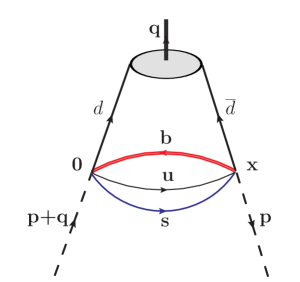
Figure 1: The leading order diagram contributing to $\Pi_{1}(p,q)$.

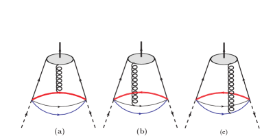
Figure 2: The one-gluon exchange diagrams giving rise to corrections, which can be computed by utilizing $\rho$-meson three-particle DAs.

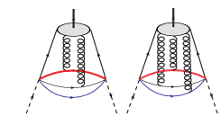
Figure 3: Some many-particle diagrams neglected in this work.

To provide some details of the calculations, as an example, we choose the term $\Pi_{1}(p,q)$. The similar consideration can also be carried our for $\Pi_{2}(p,q)$. We start our analysis from the perturbative component of $\Pi_{1}(p,q)$ (Fig. 1), i.e. from the contribution

$$\Pi_{1}^{\mathrm{pert.}}(p,q)=i\int d^{4}xe^{ipx}\varepsilon^{abc}\varepsilon^{ade}\varepsilon^{a^{\prime}b^{\prime}c^{\prime}}\varepsilon^{a^{\prime}d^{\prime}e^{\prime}}$$

$$\times\mathrm{Tr}\left[\gamma_{5}\widetilde{S}_{s}^{b^{\prime}b(\mathrm{pert.})}(x)\gamma_{5}S_{u}^{cc^{\prime}(\mathrm{pert.})}(x)\right]$$

$$\times\left[\gamma_{5}\widetilde{S}_{b}^{d^{\prime}d(\mathrm{pert.})}(-x)\gamma_{5}\right]_{\alpha\beta}\langle\rho(q)|\overline{d}_{\alpha}^{e}(x)d_{\beta}^{e^{\prime}}(0)|0\rangle.$$ (14)

It is convenient first to perform the summation over the color indices. To this end, we apply the projector onto the color singlet product of quarks fields $\frac{1}{3}\delta_{ee^{\prime}}$ by performing the replacement

$$\overline{d}_{\alpha}^{e}(x)d_{\beta}^{e^{\prime}}(0)\rightarrow\frac{1}{3}\delta_{ee^{\prime}}\overline{d}_{\alpha}(x)d_{\beta}(0),$$ (15)

and use the expansion

$$\overline{d}_{\alpha}(x)d_{\beta}(0)\equiv\frac{1}{4}\Gamma_{\beta\alpha}^{J}\overline{d}(x)\Gamma^{J}d(0),$$ (16)

where the sum runs over $J$

$$\Gamma^{J}=\mathbf{1,\ }\gamma_{5},\ \gamma_{\mu},\ i\gamma_{5}\gamma_{\mu},\ \sigma_{\mu\nu}/\sqrt{2}.$$

Substituting this expansion into Eq. (14) we obtain

$$\Pi_{1}^{\mathrm{pert.}}(p,q)=i\int d^{4}xe^{ipx}\mathrm{Tr}\left[\gamma_{5}\widetilde{S}_{s}^{(\mathrm{pert.})}(x)\gamma_{5}S_{u}^{(\mathrm{pert.})}(x)\right]$$

$$\times\mathrm{Tr}\left[\gamma_{5}\widetilde{S}_{b}^{(\mathrm{pert.})}(-x)\gamma_{5}\Gamma^{J}\right]\langle\rho(q)|\overline{d}(x)\Gamma^{J}d(0)|0\rangle.$$ (17)

Now, as an example, we analyze the nonperturbative diagram depicted in Fig. 2(b). After some manipulations we recast the corresponding function $\Pi_{1(b)}^{\mathrm{n.-pert.}}(p,q)$ into the form

$$\Pi_{1(b)}^{\mathrm{n.-pert.}}(p,q)=i\int d^{4}xe^{ipx}\mathrm{Tr}\left[\gamma_{5}\widetilde{S}_{s}^{(\mathrm{pert.})}(x)\gamma_{5}\right.$$

$$\left.\left\{-ig_{s}\int_{0}^{1}dv\frac{1}{16\pi^{2}x^{2}}\left[{\not{x}}\sigma^{\mu\nu}-4ivx^{\mu}\gamma^{\nu}\right]\right\}\right]$$

$$\times\mathrm{Tr}\left[\gamma_{5}\widetilde{S}_{b}^{(\mathrm{pert.})}(-x)\gamma_{5}\Gamma^{J}\right]\frac{1}{4}\langle\rho(q)|\overline{d}(x)\Gamma^{J}G_{\mu\nu}(vx)d(0)|0\rangle.$$

The similar analysis can be done for other nonperturbative diagrams, as well.

The sum of the $\Pi_{1}^{\mathrm{pert.}}(p,q)$ and $\Pi_{1(i)}^{\mathrm{n.-pert.}}(p,q)$ for $i=a,\ b$ and $c$ determines the first component $\Pi_{1}(p,q)$ of the correlation function. It is given as the integral of the products of the coefficient functions and non-local matrix elements

$$\langle\rho(q)|\overline{d}(x)\Gamma^{J}d(0)|0\rangle,$$

$$\langle\rho(q)|\overline{d}(x)\Gamma^{J}G_{\mu\nu}(vx)d(0)|0\rangle.$$ (19)

The matrix elements of the neutral $\rho$ meson from Eq. (19) up to an isospin factor in the overall normalization are connected with ones of the charged $\rho$ mesons, and can be expanded in terms of the corresponding distribution amplitudes. Below we provide expressions for the $\langle 0|\overline{u}(x)\Gamma^{J}d(0)|\rho(q)\rangle$ type matrix elements obtained to twist-4 accuracy and given by means of the $\rho$ meson’s two-particle DAs. For the structures $\Gamma^{J}=\mathbf{1}$ and $\mathbf{\ }\gamma_{\mu}\gamma_{5}$ we get

$$\langle 0|\overline{u}(x)d(0)|\rho(q)\rangle=-if_{\rho}^{\perp}\varepsilon\cdot xm_{\rho}^{2}\int_{0}^{1}due^{i\overline{u}qx}\psi_{3}^{\parallel}(u),$$

$$\langle 0|\overline{u}(x)\gamma_{\mu}\gamma_{5}d(0)|\rho(q)\rangle=\frac{1}{2}f_{\rho}^{\parallel}m_{\rho}\epsilon_{\mu}^{\nu\alpha\beta}\varepsilon_{\nu}q_{\alpha}x_{\beta}$$

$$\times\int_{0}^{1}due^{i\overline{u}qx}\psi_{3}^{\perp}(u),$$ (20)

whereas $\Gamma^{J}=\gamma_{\mu}\$and $\sigma_{\mu\nu}$ give

$$\langle 0|\overline{u}(x)\gamma_{\mu}d(0)|\rho(q)\rangle=f_{\rho}^{\parallel}m_{\rho}\left\{\frac{\varepsilon\cdot x}{q\cdot x}q_{\mu}\right.$$

$$\times\int_{0}^{1}due^{i\overline{u}qx}\left[\phi_{2}^{\parallel}(u)+\frac{m_{\rho}^{2}x^{2}}{4}\phi_{4}^{\parallel}(u)\right]$$

$$+\left(\varepsilon_{\mu}-q_{\mu}\frac{\varepsilon\cdot x}{q\cdot x}\right)\int_{0}^{1}due^{i\overline{u}qx}\phi_{3}^{\perp}(u)$$

$$\left.-\frac{1}{2}x_{\mu}\frac{\varepsilon\cdot x}{(q\cdot x)^{2}}m_{\rho}^{2}\int_{0}^{1}due^{i\overline{u}qx}C(u)+...\right\},$$ (21)

and

$$\langle 0|\overline{u}(x)\sigma_{\mu\nu}d(0)|\rho(q)\rangle=if_{\rho}^{\perp}\left\{\left(\varepsilon_{\mu}q_{\nu}-\varepsilon_{\nu}q_{\mu}\right)\right.$$

$$\times\int_{0}^{1}due^{i\overline{u}qx}\left[\phi_{2}^{\perp}(u)+\frac{m_{\rho}^{2}x^{2}}{4}\phi_{4}^{\perp}(u)\right]$$

$$+\frac{1}{2}\left(\varepsilon_{\mu}x_{\nu}-\varepsilon_{\nu}x_{\mu}\right)\frac{m_{\rho}^{2}}{q\cdot x}\int_{0}^{1}due^{i\overline{u}qx}\left[\psi_{4}^{\perp}(u)-\phi_{2}^{\perp}(u)\right]$$

$$\left.+\left(q_{\mu}x_{\nu}-q_{\nu}x_{\mu}\right)\frac{\varepsilon\cdot x}{(q\cdot x)^{2}}m_{\rho}^{2}\int_{0}^{1}due^{i\overline{u}qx}D(u)+...\right\}$$

respectively. Here $\overline{u}=1-u$, and $m_{\rho}$ , $\varepsilon$ are the mass of $\rho$ meson and its polarization vector. In the equations above the functions $C(u)$ and $D(u)$ denote the following combinations of the two-particle DAs

$$C(u)=\psi_{4}^{\parallel}(u)+\phi_{2}^{\parallel}(u)-2\phi_{3}^{\perp}(u),$$ (23)

$$D(u)=\phi_{3}^{\parallel}(u)-\frac{1}{2}\phi_{2}^{\perp}(u)-\frac{1}{2}\psi_{4}^{\perp}(u).$$ (24)

The twists of the distribution amplitudes are shown as subscripts in the relevant functions. As is seen, these matrix elements include the two-particle leading twist DAs $\phi_{2}^{\parallel(\perp)}(u)$, the twist-3 distribution amplitudes $\phi_{3}^{\parallel(\perp)}(u)$ and $\psi_{3}^{\parallel(\perp)}(u)$, as well as twist-4 distributions $\phi_{4}^{\parallel(\perp)}(u)$ and $\psi_{4}^{\parallel(\perp)}(u)$.

We do not write down here lengthy equalities, which express the matrix elements $\langle\rho(q)|\overline{d}(x)\Gamma^{J}G_{\mu\nu}(vx)d(0)|0\rangle$ in terms of the numerous higher twist DAs of the $\rho$ meson, and refrain from giving further information on the DAs themselves. The definitions and detailed information on properties of the distribution amplitudes of the $\rho$ and other vector mesons, as well as explicit expressions for some of their models, used also in the present work, can be found in Refs. Ball:1996tb ; Ball:1998sk ; Ball:1998ff ; Ball:2007rt ; Ball:2007zt .

Our aim is to calculate the correlation function $\Pi^{\mathrm{QCD}}(p,q)$ in terms of the DAs of the $\rho$ meson, extract the invariant amplitude $\Pi^{\mathrm{QCD}}(p^{2},p^{\prime 2})$ corresponding to the structure $p\cdot\varepsilon,$ and perform its double Borel transformation

$$\Pi^{\mathrm{QCD}}(M^{2})=\mathcal{B}_{p^{2}}(M_{1}^{2})\mathcal{B}_{p^{\prime 2}}(M_{2}^{2})\Pi^{\mathrm{QCD}}(p^{2},p^{\prime 2}).$$

After equating $\Pi^{\mathrm{QCD}}(M^{2})$ to its counterpart $\Pi^{\mathrm{Phys}}(M^{2})$ and subtracting contributions of the higher resonances and continuum states presented in Eq. (8) as the double dispersion integral, we can derive the LCSR for the strong coupling $G_{X_{b}X_{b}\rho}$.

Presenting some details of calculations in Appendix A, below we write down the final expression obtained for $\Pi_{1}^{\mathrm{QCD}}(M^{2})$

$$\Pi_{1}^{\mathrm{QCD}}(M^{2}) = \frac{m_{b}m_{\rho}}{64\pi^{4}}\int_{m_{b}^{2}}^{\infty}dse^{(m_{\rho}^{2}-4s)/4M^{2}}\left[\Gamma\left(M^{8},s\right)\right.$$ (25)

$$\left.+\Gamma\left(M^{6},s\right)+\Gamma\left(M^{4},s\right)\right].$$

Here

$$\Gamma\left(M^{8},s\right)=-2m_{b}^{3}f_{\rho}^{\parallel}M^{8}\phi_{2}^{\parallel}(\overline{u}_{0})\left(\frac{1}{s^{3}}-\frac{2m_{b}^{2}}{s^{4}}+\frac{m_{b}^{4}}{s^{5}}\right),$$ (26)

$$\Gamma\left(M^{6},s\right)=-m_{b}m_{\rho}M^{6}\left\{m_{b}^{2}m_{\rho}f_{\rho}^{\parallel}\left(\frac{m_{b}^{2}}{s^{4}}-\frac{1}{s^{3}}\right)\right.$$

$$\times\phi_{4}^{\parallel}(\overline{u}_{0})+m_{\rho}f_{\rho}^{\parallel}\left.\Bigg{[}\left(\frac{1}{s^{2}}-\frac{2m_{b}^{2}}{s^{3}}+\frac{m_{b}^{4}}{s^{4}}\right)\right.$$

$$\times\left[\mathit{I}_{1}\left(\widetilde{\Phi}_{3}^{\parallel}(\alpha),1\right)-3\mathit{I}_{1}\left(\Phi_{4}^{\parallel}(\alpha),1\right)+6\mathit{I}_{1}\left(\Phi_{4}^{\parallel}(\alpha),v\right)\right.$$

$$+3\mathit{I}_{1}\left(\widetilde{\Phi}_{4}^{\parallel}(\alpha),1\right)-\mathit{I}_{1}\left(\Psi_{4}^{\parallel}(\alpha),1\right)+2\mathit{I}_{1}\left(\Psi_{4}^{\parallel}(\alpha),v\right)$$

$$\left.+\mathit{I}_{1}\left(\widetilde{\Psi}_{4}^{\parallel}(\alpha),1\right)-\mathit{I}_{1}\left(\Phi_{3}^{\parallel}(\alpha),1\right)+2\mathit{I}_{1}\left(\Phi_{3}^{\parallel}(\alpha),v\right)\right]$$

$$\left.+8m_{b}^{2}\left(\frac{m_{b}^{2}}{s^{4}}-\frac{1}{s^{3}}\right)\mathit{I}_{2}[C(u_{0})]\right.\Bigg{]}$$

$$\left.+4m_{b}f_{\rho}^{\perp}\left(\frac{1}{s^{2}}-\frac{2m_{b}^{2}}{s^{3}}+\frac{m_{b}^{4}}{s^{4}}\right)\psi_{3}^{\parallel}(\overline{u}_{0})\right\}$$ (27)

and

$$\Gamma\left(M^{4},s\right)=m_{\rho}^{3}M^{4}\left\{f_{\rho}^{\perp}\left(\frac{1}{s}-\frac{2m_{b}^{2}}{s^{2}}+\frac{m_{b}^{4}}{s^{3}}\right)\right.$$

$$\left[3\mathit{I}_{0}\left(\Phi_{3}^{\perp}(\alpha),1\right)-2\left(\mathit{I}_{0}\left(\Phi_{4}^{\perp(3)}(\alpha),1\right)\right.\right.$$

$$\left.\left.+\mathit{I}_{0}\left(\Phi_{4}^{\perp(4)}(\alpha),1\right)\right)\right]+8m_{b}m_{\rho}f_{\rho}^{\parallel}\left(\frac{1}{s^{2}}-\frac{m_{b}^{2}}{s^{3}}\right)$$

$$\left.\times\mathit{I}_{0}\left(\Psi_{4}^{\parallel}(\alpha),k-u_{0}\right)\right\}.$$ (28)

In the formulas presented above, we introduce shorthand notations for some integrals. Namely, we use

$$\mathit{I}_{0}\left(\Phi(\alpha),k-u_{0}\right) = \int\mathcal{D}\alpha\int_{0}^{1}dv\left(k-u_{0}\right)\Phi(\alpha_{\overline{q}},\alpha_{q},\alpha_{g})$$ (29)

$$\times\theta\left(k-u_{0}\right),$$

$$\mathit{I}_{1}\left(\Phi(\alpha),f(v)\right) = \int\mathcal{D}\alpha\int_{0}^{1}dv\Phi(\alpha_{\overline{q}},\alpha_{q},\alpha_{g})$$ (30)

$$\times f(v)\delta\left(k-u_{0}\right),$$

and

$$\mathit{I}_{2}\left(C(u_{0})\right)=\int_{0}^{1-u_{0}}du^{\prime}\left(u_{0}+u^{\prime}-1\right)C\left(u^{\prime}\right).$$ (31)

In Eqs. (29), (30) and (31)

$$k=\alpha_{\overline{q}}+\alpha_{g}(1-v),$$

and the integration measure $\mathcal{D}\alpha$ is defined as

$$\int\mathcal{D}\alpha=\int_{0}^{1}d\alpha_{q}\int_{0}^{1}d\alpha_{\bar{q}}\int_{0}^{1}d\alpha_{g}\delta(1-\alpha_{q}-\alpha_{\bar{q}}-\alpha_{g}).$$

The similar calculations have been carried out to derive the second component of the correlation function $\Pi_{2}^{\mathrm{QCD}}(M^{2})$.

As we have noted above, the sum rules for the coupling $G_{X_{b}X_{b}\rho}$ can be derived after continuum subtraction. The contribution coming from the higher resonances and continuum states is written down in Eq. (8) as the double dispersion integral over the physical spectral density $\rho^{\mathrm{phys}}(s_{1},s_{2})$. The subtraction is performed invoking ideas of the quark-hadron duality, i.e. by assuming that in some regions of physical quantities $\rho^{\mathrm{phys}}(s_{1},s_{2})$ may be replaced by its theoretical counterpart $\rho^{\mathrm{QCD}}(s_{1},s_{2})$, the latter is being calculable within the perturbative QCD. The spectral density $\rho^{\mathrm{QCD}}(s_{1},s_{2})$ may be found by computing the imaginary part of the correlation function, or extracted directly from its Borel transformed expression using a technique, which is described in Refs. Belyaev:1994zk ; Aliev:2010yx ; Aliev:2011ufa ; Ball:1994 . Then the continuum subtraction can be performed in accordance with the prescriptions developed in these papers. It is based on the observation that double spectral density of the leading contributions $\sim M^{2}$, is concentrated near the diagonal $s_{1}=s_{2}$. In this case for the continuum subtraction the simple expressions can be derived, which are not sensitive to the shape of the duality region. In the case $M_{1}^{2}=M_{2}^{2}=2M^{2}$ and $u_{0}=1/2$, for example, the factor

$$\left(M^{2}\right)^{N}e^{-m^{2}/M^{2}}$$ (32)

remains in its original form if $N\leq 0$, and is replaced as

$$\left(M^{2}\right)^{N}e^{-m^{2}/M^{2}}\to\frac{1}{\Gamma(N)}\int_{m^{2}}^{s_{0}}dse^{-s/M^{2}}\left(s-m^{2}\right)^{N-1},$$ (33)

for $N>0$. The subtracted version of other expressions, which may encounter in the sum rule calculations are collected in Appendix B. In the present work we follow these procedures to perform the continuum subtraction.

III Numerical results

The sum rules for the strong couplings contain some parameters, which should be determined to carry out the numerical computations. The mass and current coupling of the exotic $X_{b}$ state, as well as the mass and decay constants of the $\rho$ meson are among the important physical parameters of the problem under consideration. The situation with the $\rho$ meson is clear, because its parameters are well known: they were extracted from experimental data or evaluated employing various nonperturbative approaches, including the LCSR method Ball:2007zt ; Agashe:2014kda . The relevant information is given in Table 1.

The parameters of the $X_{b}$ state deserve more detailed consideration. Thus, its mass $m_{X_{b}}$, decay constant $f_{X_{b}}$ and the width of the decay $X_{b}\to B_{s}\pi$ were calculated in our previous works (see, Agaev:2016mjb ; Agaev:2016ijz ) using a vector diquark-vector antidiquark type interpolating current. The same parameters were also computed in Ref. Agaev:2016urs by suggesting the molecule-type internal structure for the $X_{b}$ state.

Parameters	Values
$m_{\rho}$	$(775.26\pm 0.25)~{}\mathrm{MeV}$
$f_{\rho}^{\parallel}$	$(0.216\pm 0.003)~{}\mathrm{GeV}$
$f_{\rho}^{\perp}$	$(0.165\pm 0.009)~{}\mathrm{GeV}$
$a_{2}^{\parallel}$	$0.15\pm 0.07$
$a_{2}^{\perp}$	$0.14\pm 0.06$

Table 1: The mass, decay constants, and parameters of the $\rho$ meson leading twist DAs.

In the present study, as an intermediate stage of the full analysis, we would like to calculate the spectroscopic parameters of the $X_{b}$ state using the interpolating current adopted in the present work (see, Eq. (2)). Our predictions for the mass

$$m_{X_{b}}=(5620\pm 195)\,\mathrm{MeV},$$ (34)

found by this way, is slightly larger than one given in Ref. Agaev:2016mjb , but still in agreement with the data of the D0 Collaboration. For the current coupling $f_{X_{b}}$ we obtain

$$f_{X_{b}}=(0.14\pm 0.02)\times 10^{-2}\,\mathrm{GeV}^{4}.$$ (35)

We utilize the masses of the heavy quarks in the $\overline{MS}$ scheme

$$m_{b}(m_{b})=4.18\pm 0.03\,\mathrm{GeV},$$

$$m_{c}(m_{c})=1.275\pm 0.025\,\mathrm{GeV}.$$ (36)

The scale dependence of $m_{b}$ and $m_{c}$ is taken into account in accordance with the renormalization group evolution

$$m_{q}(\mu)=m_{q}(\mu_{0})\left[\frac{\alpha_{s}(\mu)}{\alpha_{s}(\mu_{0})}\right]^{\gamma_{q}},$$ (37)

with $\gamma_{b}=12/23$ and $\gamma_{c}=12/25$. The renormalization scale in computation of the coupling $G_{X_{b}X_{b}\rho}$ is taken equal to

$$\mu_{b}=\sqrt{m_{X_{b}}^{2}-(m_{b}+m_{s})^{2}}\simeq 3.598\,\,\mathrm{GeV}.$$ (38)

The mass of the $b$ quark is evolved to this scale by employing the two-loop QCD running coupling $\alpha_{s}(\mu)$ with $\Lambda^{(4)}=326\,\,\mathrm{MeV}$.

Another set of parameters is formed due to various distribution amplitudes of the $\rho$ meson. Indeed, the leading and higher twist DAs are the important ingredients of the LCSR expressions, and in turn, contain numerous parameters. The leading twist DAs of the longitudinally and transversely polarized $\rho$ meson are given by the formula

$$\phi_{2}^{\parallel(\perp)}(u)=6u\overline{u}\left[1+\sum_{n=2}^{\infty}a_{n}^{\parallel(\perp)}C_{n}^{3/2}(2u-1)\right],$$ (39)

where $C_{n}^{m}(z)$ are the Gegenbauer polynomials. Equation (39) is the general expression for $\phi_{2}^{\parallel(\perp)}(u)$. In our calculations we employ twist-2 DAs with only one non-asymptotic term, i.e. only the coefficients $a_{2}^{\parallel(\perp)}\neq 0$ (see, Table 1). The models for the higher twist DAs, which enter to Eqs. (27) and (28) are borrowed from Refs. Ball:2007rt ; Ball:2007zt . The values of the relevant parameters at the normalization scale $\mu_{0}=1\,\mathrm{GeV}$ can be found in Tables 1 and 2 of Ref. Ball:2007zt .

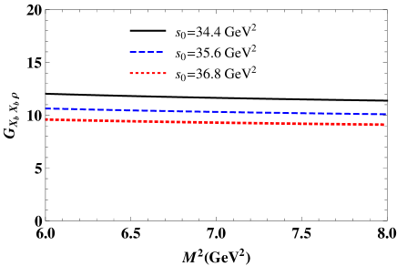
Figure 4: The strong coupling $G_{X_{b}X_{b}\rho}$ as a function of the Borel parameter $M^{2}$ at different values of $s_{0}$.

Finally, the sum rule expressions depend on two auxiliary parameters, i.e. on the Borel parameter $M^{2}$ and continuum threshold $s_{0}$, which are unavoidable within this method. Results, in general, should not depend on the choice of $M^{2}$ and $s_{0}$. In practice, however, one may only minimize effects connected with their variations. Exploring the obtained sum rules we fix working windows within of which the parameters $s_{0}$ and $M^{2}$ can be varied: for the threshold $s_{0}$ we find

$$34.4\,\,\mathrm{GeV}^{2}\leq s_{0}\leq 36.8\,\,\mathrm{GeV}^{2},$$ (40)

whereas the Borel parameter can be varied in the limits

$$6\,\,\mathrm{GeV}^{2}\leq M^{2}\leq 8\,\,\mathrm{GeV}^{2}.$$ (41)

The results of computations are depicted in Fig. 4. In accordance with our studies, the strong coupling $G_{X_{b}X_{b}\rho}$ is equal to

$$G_{X_{b}X_{b}\rho}=10.46\pm 2.26.$$ (42)

The similar analysis in the case of the vertex $X_{c}X_{c}\rho$ using the parameters of the $X_{c}$ state, namely

$$m_{X_{c}}=(2634\pm 62)\,\mathrm{MeV},$$

$$f_{X_{c}}=(0.11\pm 0.02)\times 10^{-2}\,\mathrm{GeV}^{4},$$ (43)

given in Ref. Agaev:2016lkl , restricts $s_{0}$ and $M^{2}$ inside the ranges:

$$7.6\,\mathrm{GeV}^{2} \leq s_{0}\leq 8.1\,\mathrm{GeV}^{2},$$ (44)

$$3\,\mathrm{GeV}^{2} \leq M^{2}\leq 5\,\mathrm{GeV}^{2}.$$ (45)

The scale dependence of $m_{c}$ is taken into account in accordance with Eq. (37), where

$$\mu_{c}=\sqrt{m_{X_{c}}^{2}-(m_{c}+m_{s})^{2}}\simeq 2.224\,\,\mathrm{GeV}.$$ (46)

As in the previous case, the mass of the $c$ quark is evolved to the scale $\mu_{c}$ by employing the two-loop QCD running coupling $\alpha_{s}(\mu)$.

The results of the numerical calculations are shown in Fig. 5. The QCD light-cone sum rule prediction for the strong coupling $G_{X_{c}X_{c}\rho}$ extracted in the present work reads:

$$G_{X_{c}X_{c}\rho}=8.01\pm 1.66.$$ (47)

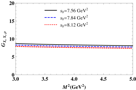
Figure 5: The coupling $G_{X_{c}X_{c}\rho}$ vs the Borel parameter $M^{2}$ at different values of $s_{0}$.

In the present work, we applied for the first time the full theory of the QCD light-cone sum rule method to systems of the tetraquarks with a single heavy quark, and calculated the strong couplings of the $X_{b}$ and $X_{c}$ states with the $\rho$ meson. To this end, we derived the sum rules by equating the Borel transformations of the same correlation function found in terms of physical quantities to its expression obtained by employing the leading and higher twist distribution amplitudes of the $\rho$ meson. We also demonstrated that technical tools elaborated for analysis of the transition form factors and strong couplings of the conventional hadrons, in general, are applicable to these complicated quark systems, as well.

Appendix A Calculation of $\Pi_{1}^{\mathrm{QCD}}(M^{2})$: some details

In this Appendix we provide some details of the calculations of the function $\Pi_{1}^{\mathrm{QCD}}(M^{2})$. To this end, we pick up a simple term from the perturbative component given by Eq. (17) and a term $\sim\phi(u)$ from the expression of the distribution amplitude. Obtained by this way integral has the form

$$I=\int_{0}^{1}du\phi(u)\int d^{4}xe^{ipx+i\overline{u}qx}\frac{1}{x^{2n}}\frac{K_{\nu}\left(m_{Q}\sqrt{-x^{2}}\right)}{\left(\sqrt{-x^{2}}\right)^{\upsilon}}.$$ (A.48)

In Eq. (A.48) the factor $1/x^{2(n_{1}+n_{2})}\equiv$ $1/x^{2n}$ is due to the light quark propagators, whereas the factor $\sim$ $K_{\nu}$ comes from the heavy quark propagator. To proceed we apply the integral representation for the Bessel functions

$$\frac{K_{\nu}\left(m_{Q}\sqrt{-x^{2}}\right)}{\left(\sqrt{-x^{2}}\right)^{\upsilon}}=\frac{1}{2}\int_{0}^{\infty}\frac{dt}{t^{\nu+1}}\exp\left[-\frac{m_{Q}}{2}\left(t-\frac{x^{2}}{t}\right)\right],$$

and perform the Wick rotation, i.e. replace $x^{2}=-\widetilde{x}^{2}$, $px\rightarrow-\widetilde{p}\widetilde{x}$, and $qx\rightarrow-\widetilde{q}\widetilde{x}$.  Finally, we make use of the Schwinger representation for the terms $1/\widetilde{x}^{2n}$

$$\frac{1}{(\widetilde{x}^{2})^{n}}=\frac{1}{\Gamma(n)}\int_{0}^{\infty}d\lambda\lambda^{n-1}\exp\left(-\lambda\widetilde{x}^{2}\right),$$

and, in what follows, omit the tilde on these variables. These replacements yield

$$I = \frac{i}{\Gamma(n)}\int_{0}^{1}du\phi(u)\int_{0}^{\infty}\frac{dt}{t^{\nu+1}}\exp\left[-\frac{m_{Q}}{2}t\right]\int_{0}^{\infty}d\lambda\lambda^{n-1}$$ (A.49)

$$\times\int d^{4}x\exp\left[-ipx-i\overline{u}qx-\lambda x^{2}-\frac{m_{Q}}{2}\frac{x^{2}}{t}\right].$$

Having shifted the variable $x$ as

$$x\rightarrow x-\frac{i(p+\overline{u}q)}{2\left(\lambda+m_{Q}/2t\right)},$$

and performed the four-dimensional Gaussian integral over the new $x$ we find

$$\int d^{4}x\exp\left[-ipx-i\overline{u}qx-\lambda x^{2}-\frac{m_{Q}}{2}\frac{x^{2}}{t}\right]$$

$$= \left(\frac{2\pi t}{m_{Q}+2\lambda t}\right)^{2}\exp\left[-\frac{t(p+\overline{u}q)^{2}}{2(m_{Q}+2\lambda t)}\right].$$

The Borel transformations of the integral $I$ give

$$I\sim\frac{i}{\Gamma(n)}\int_{0}^{1}du\phi(u)\int_{0}^{\infty}\frac{dt}{t^{\nu+1}}e^{-\frac{m_{Q}}{2}t}\int_{0}^{\infty}d\lambda\lambda^{n-1}$$

$$\times\exp\left[\frac{tu\overline{u}}{2(m_{Q}+2\lambda t)}q^{2}\right]\delta\left(\frac{1}{M_{1}^{2}}-\frac{tu}{2(m_{Q}+2\lambda t)}\right)$$

$$\times\delta\left(\frac{1}{M_{2}^{2}}-\frac{t\overline{u}}{2(m_{Q}+2\lambda t)}\right).$$ (A.50)

Now using

$$\delta\left(\frac{1}{M_{1}^{2}}-\frac{tu}{2(m_{Q}+2\lambda t)}\right)=\frac{M_{1}^{4}u}{4}\delta(\lambda-\lambda_{0})\theta(\lambda_{0}),$$ (A.51)

where $\lambda_{0}$ equals to

$$\frac{M_{1}^{2}tu-2m_{Q}}{4t},$$ (A.52)

we carry out the $\lambda$ integration. The next step is computation of the $u$ integral. To this end, we employ the second delta function and transform it as

$$\delta\left(\frac{1}{M_{2}^{2}}-\frac{t\overline{u}}{2(m_{Q}+2\lambda_{0}t)}\right)=\frac{M_{1}^{2}M_{2}^{4}}{\left(M_{1}^{2}+M_{2}^{2}\right)^{2}}\delta(u-u_{0}),$$

where

$$u_{0}=\frac{M_{2}^{2}}{M_{1}^{2}+M_{2}^{2}}.$$

The integration over $u$ sets $\phi(u)\rightarrow\phi(u_{0})$, and also determines the low limit of the remaining $t$ integral, which has become equal to

$$t_{\min}=\frac{2m_{Q}}{M_{1}^{2}u_{0}}.$$

By re-scaling the variable $t$

$$t\rightarrow\frac{2}{M_{1}^{2}u_{0}}\frac{s}{m_{Q}},$$

we obtain the integral over $s$ running from $m_{Q}^{2}$ till infinity, and, by this way, the considering component of $\Pi_{1}^{\mathrm{QCD}}(M^{2})$ takes its final form.

Appendix B The formulas for the continuum subtraction

Here we have collected useful formulas, which can be applied in the continuum subtraction. In the left-hand side of the formulas presented below we write down the original form, and in the right-hand side the subtracted version of expressions encountered in the sum rule calculations:

$$\left(M^{2}\right)^{N}\int_{m^{2}}^{\infty}dse^{-s/M^{2}}f(s)\rightarrow\int_{m^{2}}^{s_{0}}dse^{-s/M^{2}}F_{N}(s).$$ (B.53)

For the more complicated factor

$$\left(M^{2}\right)^{N}\ln\left(\frac{M^{2}}{\Lambda^{2}}\right)\int_{m^{2}}^{\infty}dse^{-s/M^{2}}f(s),$$ (B.54)

for all values of $N$ the following formula is valid

$$\int_{m^{2}}^{s_{0}}dse^{-s/M^{2}}\left[F_{N}(m^{2})\ln\left(\frac{s-m^{2}}{\Lambda^{2}}\right)+\gamma_{E}F_{N}(s)\right.$$

$$\left.+\int_{m^{2}}^{s}duF_{N-1}(u)\ln\left(\frac{s-u}{\Lambda^{2}}\right)\right].$$ (B.55)

The next formula is

$$\left(M^{2}\right)^{N}\ln\left(\frac{M^{2}}{\Lambda^{2}}\right)e^{-m^{2}/M^{2}}$$

$$\rightarrow e^{-s_{0}/M^{2}}\sum_{i=1}^{1-N}\left(\frac{d}{ds_{0}}\right)^{1-N-i}\left[\ln\left(\frac{s_{0}-m^{2}}{\Lambda^{2}}\right)\right]\frac{1}{\left(M^{2}\right)^{i-1}}$$

$$+\gamma_{E}\left(M^{2}\right)^{N}\left(e^{-m^{2}/M^{2}}-\delta_{N1}e^{-s_{0}/M^{2}}\right)$$

$$+\left(M^{2}\right)^{N-1}\int_{m^{2}}^{s_{0}}dse^{-s/M^{2}}\ln\left(\frac{s-m^{2}}{\Lambda^{2}}\right),$$ (B.56)

if $N\leq 1$, and

$$\frac{\gamma_{E}}{\Gamma(N)}\int_{m^{2}}^{s_{0}}dse^{-s/M^{2}}\left(s-m^{2}\right)^{N-1}$$

$$+\frac{1}{\Gamma(N-1)}\int_{m^{2}}^{s_{0}}dse^{-s/M^{2}}\int_{m^{2}}^{s}du(s-u)^{N-2}$$

$$\times\ln\left(\frac{u-m^{2}}{\Lambda^{2}}\right),$$ (B.57)

for $N>1$.

Useful are also the expressions

$$\left(M^{2}\right)^{N}\int_{m^{2}}^{\infty}dse^{-s/M^{2}}f(s)\ln\left(\frac{s-m^{2}}{\Lambda^{2}}\right)$$

$$\rightarrow e^{-s_{0}/M^{2}}\sum_{i=1}^{|N|}\frac{\widetilde{F}_{N+i}(s_{0})}{\left(M^{2}\right)^{i-1}}+\left(M^{2}\right)^{N}\int_{m^{2}}^{s_{0}}dse^{-s/M^{2}}f(s)$$

$$\times\ln\left(\frac{s-m^{2}}{\Lambda^{2}}\right),\ \ \ N\leq 0,$$ (B.58)

and

$$\frac{1}{\Gamma(N)}\int_{m^{2}}^{s_{0}}dse^{-s/M^{2}}\int_{m^{2}}^{s}du(s-u)^{N-1}$$

$$\times\ln\left(\frac{u-m^{2}}{\Lambda^{2}}\right)f(u),\ \ N>0.$$ (B.59)

In the equations above we have employed the notations

$$F_{N}(s)=\left(\frac{d}{ds}\right)^{-N}f(s),\,\,\,N\leq 0,$$ (B.60)

and

$$F_{N}(s)=\frac{1}{\Gamma(N)}\int_{m^{2}}^{s}du(s-u)^{N-1}f(u),\,\,\,N>0.$$ (B.61)

For $N\leq 0$ we have also used:

$$\widetilde{F}_{N}(s)=\left(\frac{d}{ds}\right)^{-N}\left[f(s)\int_{1}^{\infty}\frac{dt}{t}\exp\left(-\frac{\Lambda^{2}t}{s-m^{2}}\right)\right],$$

$$\widetilde{F}_{N}(s_{0})=\left(\frac{d}{ds_{0}}\right)^{-N}\left[f(s_{0})\ln\left(\frac{s_{0}-m^{2}}{\Lambda^{2}}\right)-\gamma_{E}\right].$$

The expression provided above are valid only if $f(m^{2})=0$. In other cases, one has to use the prescription $f(s)=[f(s)-f(m^{2})]+f(m^{2})$, where the first term in the brackets is equal to zero, when $s=m^{2}$.

References

(1) S. K. Choi et al. [Belle Collaboration],
Phys. Rev. Lett. 91, 262001 (2003).
(2) V. M. Abazov et al. [D0 Collaboration],
Phys. Rev. Lett.
textbf93, 162002 (2004).
(3) D. Acosta et al. [CDF Collaboration],
Phys. Rev. Lett. 93, 072001 (2004).
(4) B. Aubert et al. [BaBar Collaboration],
Phys. Rev. D 71, 071103 (2005).
(5)
R. L. Jaffe, Phys. Rept. 409, 1 (2005).
(6) E. S. Swanson,
Phys. Rept. 429, 243 (2006).
(7) E. Klempt and A. Zaitsev,
Phys. Rept. 454, 1 (2007).
(8) S. Godfrey and S. L. Olsen,
Ann. Rev. Nucl. Part. Sci. 58, 51 (2008).
(9) M. B. Voloshin, Prog. Part. Nucl. Phys. 61, 455 (2008).
(10) M. Nielsen, F. S. Navarra and S. H. Lee,
Phys. Rept. 497, 41 (2010).
(11) R. Faccini, A. Pilloni and A. D. Polosa,
Mod. Phys. Lett. A 27, 1230025 (2012).
(12) A. Esposito, A. L. Guerrieri, F. Piccinini,
Int. J. Mod. Phys. A 30, 1530002 (2014).
(13) H.-X. Chen, W. Chen, X. Liu, and S.-L. Zhu,
arXiv: 1601.02092 [hep-ph].
(14) V. M. Abazov et al. [D0 Collaboration],
arXiv:1602.07588 [hep-ex].
(15) The LHCb Collaboration (LHCb Collaboration),
LHCb-CONF-2016-004, CERN-LHCb-CONF-2016-004.
(16) S. S. Agaev, K. Azizi and H. Sundu,
Phys. Rev. D 93, 074024 (2016).
(17) Z. G. Wang,
arXiv:1602.08711 [hep-ph].
(18) W. Wang and R. Zhu,
arXiv:1602.08806 [hep-ph].
(19) W. Chen, H. X. Chen, X. Liu, T. G. Steele and
S. L. Zhu,
arXiv:1602.08916 [hep-ph].
(20) C. M. Zanetti, M. Nielsen and K. P. Khemchandani,
arXiv:1602.09041 [hep-ph].
(21) S. S. Agaev, K. Azizi and H. Sundu,
Phys. Rev. D 93, 114007 (2016).
(22) S. S. Agaev, K. Azizi and H. Sundu,
Phys. Rev. D 93, 074002 (2016).
(23) J. M. Dias, K. P. Khemchandani, A. M. Torres,
M. Nielsen and C. M. Zanetti,
arXiv:1603.02249 [hep-ph].
(24) Z. G. Wang,
arXiv:1603.02498 [hep-ph].
(25) C. J. Xiao and D. Y. Chen,
arXiv:1603.00228 [hep-ph].
(26) S. S. Agaev, K. Azizi and H. Sundu,
arXiv:1603.02708 [hep-ph].
(27) S. S. Agaev, K. Azizi and H. Sundu,
Phys. Rev. D 93, 094006 (2016).
(28) Y. R. Liu, X. Liu and S. L. Zhu,
arXiv:1603.01131 [hep-ph].
(29) X. G. He and P. Ko,
arXiv:1603.02915 [hep-ph].
(30) Y. Jin and S. Y. Li,
arXiv:1603.03250 [hep-ph].
(31) F. Stancu,
arXiv:1603.03322 [hep-ph].
(32) T. J. Burns and E. S. Swanson,
arXiv:1603.04366 [hep-ph].
(33) L. Tang and C. F. Qiao,
arXiv:1603.04761 [hep-ph].
(34) F. K. Guo, U. G. Mei?ner and B. S. Zou,
arXiv:1603.06316 [hep-ph].
(35) Q. F. Lu and Y. B. Dong,
arXiv:1603.06417 [hep-ph].
(36) A. Esposito, A. Pilloni and A. D. Polosa,
arXiv:1603.07667 [hep-ph].
(37) M. Albaladejo, J. Nieves, E. Oset, Z. F. Sun
and X. Liu,
arXiv:1603.09230 [hep-ph].
(38) A. Ali, L. Maiani, A. D. Polosa and V. Riquer,
arXiv:1604.01731 [hep-ph].
(39) I. I. Balitsky, V. M. Braun and
A. V. Kolesnichenko,
Nucl. Phys. B 312, 509 (1989).
(40) V. M. Belyaev, V. M. Braun, A. Khodjamirian and
R. Ruckl, Phys. Rev. D 51, 6177 (1995).
(41) T. M. Aliev, D. A. Demir, E. Iltan and N. K. Pak,
Phys. Rev. D 53, 355 (1996).
(42) A. Khodjamirian, R. Ruckl, S. Weinzierl and
O. I. Yakovlev,
Phys. Lett. B 457, 245 (1999).
(43)
T. M. Aliev, K. Azizi and M. Savci,
Phys. Lett. B 696, 220 (2011).
(44)
T. M. Aliev, K. Azizi and M. Savci,
Nucl. Phys. A 870-871, 58 (2011).
(45) S. S. Agaev, K. Azizi and H. Sundu,
Phys. Rev. D 92, 116010 (2015).
(46) P. Ball and V. M. Braun,
Phys. Rev. D 54, 2182 (1996).
(47) P. Ball, V. M. Braun, Y. Koike and K. Tanaka,
Nucl. Phys. B 529, 323 (1998).
(48) P. Ball and V. M. Braun,
Nucl. Phys. B 543, 201 (1999).
(49) P. Ball and G. W. Jones,
JHEP 0703, 069 (2007).
(50) P. Ball, V. M. Braun and A. Lenz,
JHEP 0708, 090 (2007).
(51) P. Ball, V. M. Braun, Phys. Rev. D 49, 2472
(1994).
(52)
K. A. Olive et al. [Particle Data Group Collaboration],
Chin. Phys. C 38, 090001 (2014).