Estimates for the upscaling error in heterogeneous multiscale methods for wave propagation problems in locally periodic media

Doghonay Arjmand  and  Olof Runborg doghonay.arjmand@it.uu.se,olofr@kth.se Division of Scientific Computing
Department of Information Technology
Uppsala University
SE-751 05 Uppsala, Sweden.
Division of numerical analysis
Department of Mathematics
The Royal Institute of Technology
Stockholm, Sweden.
Abstract.

This paper concerns the analysis of a multiscale method for wave propagation problems in microscopically nonhomogeneous media. A direct numerical approximation of such problems is prohibitively expensive as it requires resolving the microscopic variations over a much larger physical domain of interest. The heterogeneous multiscale method (HMM) is an efficient framework to approximate the solutions of multiscale problems. In HMM, one assumes an incomplete macroscopic model which is coupled to a known but expensive microscopic model. The micromodel is solved only locally to upscale the parameter values which are missing in the macromodel. The resulting macroscopic model can then be solved at a cost independent of the small scales in the problem.

In general, the accuracy of the HMM is related to how good the upscaling step approximates the right macroscopic quantities. The analysis of the method, that we consider here, was previously addressed only in purely periodic media although the method itself is numerically shown to be applicable to more general settings. In the present study, we consider a more realistic setting by assuming a locally-periodic medium where slow and fast variations are allowed at the same time. We then prove that HMM captures the right macroscopic effects. The generality of the tools and ideas in the analysis allows us to establish convergence rates in a multi-dimensional setting. The theoretical findings here imply an improved convergence rate in one-dimension, which also justifies the numerical observations from our earlier study.

Key words and phrases:
multiscale methods, homogenization, wave propagation

1. Introduction

We consider the scalar wave equation in locally-periodic media

(1) ttuε(t,𝐱)subscript𝑡𝑡superscript𝑢𝜀𝑡𝐱\displaystyle\partial_{tt}u^{\varepsilon}(t,{\bf x}) =(A(𝐱,𝐱/ε)uε(t,𝐱))+f(t,𝐱), in Ω×(0,T]absent𝐴𝐱𝐱𝜀superscript𝑢𝜀𝑡𝐱𝑓𝑡𝐱 in Ω0𝑇\displaystyle=\nabla\cdot\Big{(}A({\bf x},{\bf x}/\varepsilon)\nabla u^{\varepsilon}(t,{\bf x})\Big{)}+f(t,{\bf x}),\quad\text{ in }\Omega\times(0,T]
uε(0,𝐱)superscript𝑢𝜀0𝐱\displaystyle u^{\varepsilon}(0,{\bf x}) =g(𝐱),tuε(0,𝐱)=h(𝐱), on Ω×{t=0},formulae-sequenceabsent𝑔𝐱subscript𝑡superscript𝑢𝜀0𝐱𝐱 on Ω𝑡0\displaystyle=g({\bf x}),\quad\partial_{t}u^{\varepsilon}(0,{\bf x})=h({\bf x}),\quad\text{ on }\Omega\times\{t=0\},
uε(t,𝐱)superscript𝑢𝜀𝑡𝐱\displaystyle u^{\varepsilon}(t,{\bf x}) =0 on Ω×[0,T],absent0 on Ω0𝑇\displaystyle=0\quad\text{ on }\partial\Omega\times[0,T],

where ΩΩ\Omega is a bounded open subset of dsuperscript𝑑\mathbb{R}^{d} with |Ω|=O(1)Ω𝑂1|\Omega|=O(1), and A𝐴A is a bounded symmetric positive-definite matrix function in d×dsuperscript𝑑𝑑\mathbb{R}^{d\times d} such that for every ζd𝜁superscript𝑑{\bf{\zeta}}\in\mathbb{R}^{d}

c1|ζ|2sup𝐱Ω,𝐲YζTA(𝐱,𝐲)ζc2|ζ|2,Y=(0,1]d, and Aij=Aji.formulae-sequencesubscript𝑐1superscript𝜁2subscriptsupremumformulae-sequence𝐱Ω𝐲𝑌superscript𝜁𝑇𝐴𝐱𝐲𝜁subscript𝑐2superscript𝜁2formulae-sequence𝑌superscript01𝑑 and subscript𝐴𝑖𝑗subscript𝐴𝑗𝑖c_{1}|{\bf{\zeta}}|^{2}\leq\sup_{{\bf x}\in\Omega,{\bf y}\in Y}\zeta^{T}A({\bf x},{\bf y}){\bf{\zeta}}\leq c_{2}\left|{\bf{\zeta}}\right|^{2},\quad Y=(0,1]^{d},\text{ and }A_{ij}=A_{ji}.

The coefficient A𝐴A is assumed to be locally-periodic, i.e. 𝐲A(𝐱,𝐲)𝐲𝐴𝐱𝐲{\bf y}\longrightarrow A({\bf x},{\bf y}) is Y𝑌Y-periodic for all 𝐱𝐱{\bf x} in ΩΩ\Omega, the parameter ε1much-less-than𝜀1\varepsilon\ll 1 represents the wavelength of the small scale variations in the media, and T=O(1)𝑇𝑂1T=O(1) is a constant independent of ε𝜀\varepsilon. For simplicity, we will assume that A𝐴A is smooth, i.e., AijC(Ω¯×Y¯)subscript𝐴𝑖𝑗superscript𝐶¯Ω¯𝑌A_{ij}\in C^{\infty}(\overline{\Omega}\times\overline{Y}), but most of the theoretical results in this paper will be valid for less regular coefficients such as 𝐱kAijC(Ω¯,L(Y))superscriptsubscript𝐱𝑘subscript𝐴𝑖𝑗𝐶¯Ωsuperscript𝐿𝑌\partial_{{\bf x}}^{k}A_{ij}\in C(\overline{\Omega},L^{\infty}(Y)) for k2𝑘2k\leq 2.

When ε1much-less-than𝜀1\varepsilon\ll 1, the solution to equation (1) exhibits variations at a coarse and a fine scale, in time and space, due to the heterogeneities in the coefficient function A𝐴A. In this case, a direct numerical simulation (DNS) of (1) becomes highly demanding since ε𝜀\varepsilon-scale variations must be resolved over the entire domain, leading to O(εd1)𝑂superscript𝜀𝑑1O(\varepsilon^{-d-1}) degrees of freedom. Although DNS provides us with detailed information about the behavior of the solution at different scales, in engineering practices, we are often interested only in a coarse scale description of the solution. This raises the following question: can we approximate the coarse scale, i.e. a local average, part of the solution at a cost much lower than the cost of DNS? From a mathematical point of view this is related to the theory of homogenization which can be traced back to 197019701970s. On the other hand, from a numerical point of view, this issue has triggered the birth and development of a number of successful numerical multiscale approaches over the last two decades.

First we give a brief summary of the idea behind analytical homogenization. The term homogenization was introduced to the mathematical literature by I. Babuska, [11] and since then the theory has been systematically developed by contributions of various researchers, see e.g. [13, 15, 34, 39] for an exposition of the method, where references to earlier literature can also be found. Mathematically speaking, the aim of the homogenization theory is to find a limiting solution uεu0superscript𝑢𝜀superscript𝑢0u^{\varepsilon}\longrightarrow u^{0}, in some appropriate sense, and possibly a homogenized problem, satisfied by u0superscript𝑢0u^{0}, which is no more dependent on the small scale parameter ε𝜀\varepsilon. In a few cases, it is possible to write down explicit equations for the homogenized problem. For example, when the medium is periodic or locally periodic, the homogenized solution u0superscript𝑢0u^{0} solves

(2) ttu0(t,𝐱)subscript𝑡𝑡superscript𝑢0𝑡𝐱\displaystyle\partial_{tt}u^{0}(t,{\bf x}) =(A0(𝐱)u0(t,𝐱))+f(t,𝐱), in Ω×(0,T]absentsuperscript𝐴0𝐱superscript𝑢0𝑡𝐱𝑓𝑡𝐱 in Ω0𝑇\displaystyle=\nabla\cdot\Big{(}A^{0}({\bf x})\nabla u^{0}(t,{\bf x})\Big{)}+f(t,{\bf x}),\quad\text{ in }\Omega\times(0,T]
u0(0,𝐱)superscript𝑢00𝐱\displaystyle u^{0}(0,{\bf x}) =g(𝐱),tu0(0,𝐱)=h(𝐱), on Ω×{t=0},formulae-sequenceabsent𝑔𝐱subscript𝑡superscript𝑢00𝐱𝐱 on Ω𝑡0\displaystyle=g({\bf x}),\quad\partial_{t}u^{0}(0,{\bf x})=h({\bf x}),\quad\text{ on }\Omega\times\{t=0\},

where the homogenized matrix A0superscript𝐴0A^{0} is given by

(3) Aij0(𝐱)=Y(Aij(𝐱,𝐲)+k=1dAikykχj(𝐱,𝐲))𝑑𝐲,subscriptsuperscript𝐴0𝑖𝑗𝐱subscript𝑌subscript𝐴𝑖𝑗𝐱𝐲superscriptsubscript𝑘1𝑑subscript𝐴𝑖𝑘subscriptsubscript𝑦𝑘subscript𝜒𝑗𝐱𝐲differential-d𝐲A^{0}_{ij}({\bf x})=\int_{Y}\left(A_{ij}({\bf x},{\bf y})+\sum_{k=1}^{d}A_{ik}\partial_{y_{k}}\chi_{j}({\bf x},{\bf y})\right)\;d{\bf y},

and {χ}=1dsuperscriptsubscriptsubscript𝜒1𝑑\{\chi_{\ell}\}_{\ell=1}^{d} are Y𝑌Y-periodic solutions of the following set of cell problems

(4) 𝐲(A(𝐱,𝐲)𝐲χ(𝐱,𝐲)+A(𝐱,𝐲)e)=0,Yχ(𝐱,𝐲)𝑑𝐲=0,formulae-sequencesubscript𝐲𝐴𝐱𝐲subscript𝐲subscript𝜒𝐱𝐲𝐴𝐱𝐲subscript𝑒0subscript𝑌subscript𝜒𝐱𝐲differential-d𝐲0\displaystyle\nabla_{{\bf y}}\cdot\left(A({\bf x},{\bf y})\nabla_{{\bf y}}\chi_{\ell}({\bf x},{\bf y})+A({\bf x},{\bf y})e_{\ell}\right)=0,\quad\int_{Y}\chi_{\ell}({\bf x},{\bf y})\;d{\bf y}=0,

where {e}=1dsuperscriptsubscriptsubscript𝑒1𝑑\{e_{\ell}\}_{\ell=1}^{d} are canonical basis vectors in dsuperscript𝑑\mathbb{R}^{d}. Although the homogenization theory provides us with powerful analytical tools to study existence and uniqueness of homogenized solutions, it is of limited practical use since an explicit representation for the homogenized coefficient A0superscript𝐴0A^{0} is often missing. In such a case, the tendency is to design multiscale numerical methods which target the coarse scale behavior of the solution, i.e., the homogenized solution, without assuming a priori knowledge about the homogenized coefficient or the precise nature of the coefficient A𝐴A. Within the last two decades, several multiscale strategies have been proposed to approximate the coarse-scale dynamics of problems which possess variations at multiple scales. To name a few, the variational multiscale method (VMM) pioneered by Hughes et al. [33], the multiscale finite element method (MsFEM) by T. Hou et al. [31], the equation-free approach by Kevrikidis et al. [35], and the heterogeneous multiscale method (HMM) due to E and Engquist [17] are successful examples of such general frameworks. Due to the large literature available on these methodologies, at this stage, we refer the curious reader only to few representative works in the context of applications to multiscale PDEs, see e.g. [5, 28, 36] for methods inspired by the VMM principle, [19, 20, 32, 29] for MsFEM type methods, and [10, 21, 4] for HMM based strategies. See also [12, 23, 25, 26, 37, 38, 42] for other relevant literatures on multiscale approaches for PDEs.

The focus of the present work is on the HMM strategy. The idea behind HMM is to assume a macroscale model which lacks certain input data. To close the macromodel, one then solves a micromodel locally and computes effective parameter values needed for the macromodel. Since the micromodel is solved only locally, the approach leads to a significant improvement in terms of computational cost in comparison to traditional numerical schemes. HMM has been applied to a wide range of multiscale problems, see e.g. [1, 6, 9, 10, 18] for elliptic, parabolic and second-order hyperbolic PDEs, [40] for applications in micro-fluidics, [24, 16] for applications in ODEs with multiple scales, and [3] for a recent overview of the method.

In [17, 3], a general framework for the analysis of HMM for multiscale PDEs is given. The idea is to split the error between the HMM and the homogenized solution (2) into three parts

|UHMMu0|=emacro+eupscaling+emicro,subscript𝑈𝐻𝑀𝑀superscript𝑢0subscript𝑒𝑚𝑎𝑐𝑟𝑜subscript𝑒𝑢𝑝𝑠𝑐𝑎𝑙𝑖𝑛𝑔subscript𝑒𝑚𝑖𝑐𝑟𝑜\displaystyle\left|U_{HMM}-u^{0}\right|=e_{macro}+e_{upscaling}+e_{micro},

where emacrosubscript𝑒𝑚𝑎𝑐𝑟𝑜e_{macro} and emicrosubscript𝑒𝑚𝑖𝑐𝑟𝑜e_{micro} are discretization errors, and eupscalingsubscript𝑒𝑢𝑝𝑠𝑐𝑎𝑙𝑖𝑛𝑔e_{upscaling} or so-called the HMM error is related to the accuracy of upscaling procedure where effective parameters in the macromodel are computed using local microscopic simulations, see Remark 4. The aim of this study is to estimate the difference between the upscaled effective parameters and the exact homogenized quantities. A fully discrete analysis of a finite element HMM for elliptic PDEs can be found e.g. in [1]. The analysis of the discretization errors is omitted in the present work and can be carried out using standard theory of finite differences or finite elements, see e.g. [14, 27, 41].

In this paper, we analyze a finite difference HMM (FD-HMM) from [21] which approximates the solution of the second order wave equation (1), see Section 2 for a summary of the FD-HMM. The analysis of this FD-HMM in purely periodic media was previously addressed in [21] for short time problems where T=O(1)𝑇𝑂1T=O(1), and in [8, 22] for long time scales where T=O(ε2)𝑇𝑂superscript𝜀2T=O(\varepsilon^{-2}). To be able to go beyond the rather academic case of periodic media and to address a more realistic scenario, an extension of the theory to non-periodic media is needed. The difficulty lies in the fact that existing theoretical results in the periodic case do not directly apply to non-periodic media. The analysis in this paper does not fully cover the general non-periodic theory, but is based on two main assumptions: i) as a special case of non-periodic coefficients, locally-periodic coefficients, see the coefficient A𝐴A in (1), are assumed. ii) A scale separation, ε1much-less-than𝜀1\varepsilon\ll 1, in the coefficient A𝐴A (and hence in the solution) is assumed.

This article is structured as follows. In Section 2, we introduce the multiscale method. A detailed analysis of the method is then given in Section 4. We finish the article by a conclusion in Section 5.

2. HMM

The FD-HMM uses the following macromodel for approximating the solution of problem (1)

(5) Macro problem: ttU(t,𝐱)𝐅(𝐱,U)=f(𝐱), in Ω×(0,T]U(0,𝐱)=g(𝐱),tU(0,𝐱)=h(𝐱), on Ω×{t=0},U(t,𝐱)=0, on Ω×[0,T].Macro problem: subscript𝑡𝑡𝑈𝑡𝐱𝐅𝐱𝑈𝑓𝐱 in Ω0𝑇missing-subexpressionmissing-subexpressionformulae-sequence𝑈0𝐱𝑔𝐱subscript𝑡𝑈0𝐱𝐱 on Ω𝑡0missing-subexpressionmissing-subexpression𝑈𝑡𝐱0 on Ω0𝑇missing-subexpressionmissing-subexpression\text{Macro problem: }\begin{array}[]{lll}\partial_{tt}U(t,{\bf x})-\nabla\cdot{\bf F}({\bf x},\nabla U)=f({\bf x}),\quad\text{ in }\Omega\times(0,T]\\ U(0,{\bf x})=g({\bf x}),\quad\partial_{t}U(0,{\bf x})=h({\bf x}),\quad\text{ on }\Omega\times\{t=0\},\\ U(t,{\bf x})=0,\quad\text{ on }\partial\Omega\times[0,T].\end{array}

Here U𝑈U is the macroscopic solution and 𝐅=(F1,F2,,Fd)𝐅superscript𝐹1superscript𝐹2superscript𝐹𝑑{\bf F}=(F^{1},F^{2},\cdots,F^{d}) is the missing data in the model. A finite difference discretization (in two dimensions) of the macro problem (5) gives

(6) Ui,jn+1=2Ui,jnUi,jn1+t2(Fi+12,j1,nFi12,j1,nH+Fi,j+122,nFi,j122,nH)+t2fi,jn.superscriptsubscript𝑈𝑖𝑗𝑛12superscriptsubscript𝑈𝑖𝑗𝑛superscriptsubscript𝑈𝑖𝑗𝑛1superscript𝑡2superscriptsubscript𝐹𝑖12𝑗1𝑛superscriptsubscript𝐹𝑖12𝑗1𝑛𝐻superscriptsubscript𝐹𝑖𝑗122𝑛superscriptsubscript𝐹𝑖𝑗122𝑛𝐻superscript𝑡2superscriptsubscript𝑓𝑖𝑗𝑛missing-subexpression\begin{array}[]{ll}U_{i,j}^{n+1}=2U_{i,j}^{n}-U_{i,j}^{n-1}+\triangle t^{2}\left(\dfrac{F_{i+\frac{1}{2},j}^{1,n}-F_{i-\frac{1}{2},j}^{1,n}}{H}+\dfrac{F_{i,j+\frac{1}{2}}^{2,n}-F_{i,j-\frac{1}{2}}^{2,n}}{H}\right)+\triangle t^{2}f_{i,j}^{n}.\end{array}

Moreover, Ui,j0=gi,jsubscriptsuperscript𝑈0𝑖𝑗subscript𝑔𝑖𝑗U^{0}_{i,j}=g_{i,j}, and Ui,j1subscriptsuperscript𝑈1𝑖𝑗U^{1}_{i,j} is given by

Ui,j1subscriptsuperscript𝑈1𝑖𝑗\displaystyle U^{1}_{i,j} U(t,𝐱i,j)U(0,𝐱i,j)+ttU(0,𝐱i,j)+t22ttU(0,𝐱i,j),absent𝑈𝑡subscript𝐱𝑖𝑗𝑈0subscript𝐱𝑖𝑗𝑡subscript𝑡𝑈0subscript𝐱𝑖𝑗superscript𝑡22subscript𝑡𝑡𝑈0subscript𝐱𝑖𝑗\displaystyle\approx U(\triangle t,{\bf x}_{i,j})\approx U(0,{\bf x}_{i,j})+\triangle t\partial_{t}U(0,{\bf x}_{i,j})+\dfrac{\triangle t^{2}}{2}\partial_{tt}U(0,{\bf x}_{i,j}),

where the initial data in (5) can be used to compute the first two terms in the right hand side, and the last term is computed by using the equation (5) which also requires computing 𝐅𝐅{\bf F} at time t=0𝑡0t=0. To compute the unknown 𝐅i+12,jnsuperscriptsubscript𝐅𝑖12𝑗𝑛{\bf F}_{i+\frac{1}{2},j}^{n} in the macro solver (6), we solve the multiscale problem (1) over a microscopic box Iτ×Ω𝐱i+1/2,jsubscript𝐼𝜏subscriptΩsubscript𝐱𝑖12𝑗I_{\tau}\times\Omega_{{\bf x}_{i+1/2,j}}, where Iτ=(0,τ/2]subscript𝐼𝜏0𝜏2I_{\tau}=(0,\tau/2] and τ/2𝜏2\tau/2 is the final time for the microscopic simulations, and Ω𝐱i+1/2,j,η:=𝐱i+1/2,j+[Lη,Lη]dassignsubscriptΩsubscript𝐱𝑖12𝑗𝜂subscript𝐱𝑖12𝑗superscriptsubscript𝐿𝜂subscript𝐿𝜂𝑑\Omega_{{\bf x}_{i+1/2,j},\eta}:={\bf x}_{i+1/2,j}+[-L_{\eta},L_{\eta}]^{d} where Lηη2+τ2|A|subscript𝐿𝜂𝜂2𝜏2subscript𝐴L_{\eta}\geq\frac{\eta}{2}+\frac{\tau}{2}\sqrt{|A|_{\infty}} and in practice τ=η=O(ε)𝜏𝜂𝑂𝜀\tau=\eta=O(\varepsilon). In other words, we solve

(7) Micro problem: ttuε,η(t,𝐱)(A(𝐱,𝐱/ε)uε,η)=0, in Ω𝐱i+1/2,j,η×Iτuε,η(0,𝐱)=u^(𝐱),tuε,η(0,𝐱)=0, on Ω𝐱i+1/2,j,η×{t=0},uε,η(0,𝐱)u^(𝐱) is periodic in Ω𝐱i+1/2,j,η.Micro problem: subscript𝑡𝑡superscript𝑢𝜀𝜂𝑡𝐱𝐴𝐱𝐱𝜀superscript𝑢𝜀𝜂0 in subscriptΩsubscript𝐱𝑖12𝑗𝜂subscript𝐼𝜏missing-subexpressionmissing-subexpressionformulae-sequencesuperscript𝑢𝜀𝜂0𝐱^𝑢𝐱subscript𝑡superscript𝑢𝜀𝜂0𝐱0 on subscriptΩsubscript𝐱𝑖12𝑗𝜂𝑡0missing-subexpressionmissing-subexpressionsuperscript𝑢𝜀𝜂0𝐱^𝑢𝐱 is periodic in subscriptΩsubscript𝐱𝑖12𝑗𝜂missing-subexpressionmissing-subexpression\text{Micro problem: }\begin{array}[]{lll}\partial_{tt}u^{\varepsilon,\eta}(t,{\bf x})-\nabla\cdot\left(A({\bf x},{\bf x}/\varepsilon)\nabla u^{\varepsilon,\eta}\right)=0,\text{ in }\Omega_{{\bf x}_{i+1/2,j},\eta}\times I_{\tau}\\ u^{\varepsilon,\eta}(0,{\bf x})=\hat{u}({\bf x}),\quad\partial_{t}u^{\varepsilon,\eta}(0,{\bf x})=0,\quad\text{ on }{\Omega_{{\bf x}_{i+1/2,j},\eta}}\times\{t=0\},\\ u^{\varepsilon,\eta}(0,{\bf x})-\hat{u}({\bf x})\quad\text{ is periodic in }\Omega_{{\bf x}_{i+1/2,j},\eta}.\end{array}

where u^(𝐱)^𝑢𝐱\hat{u}({\bf x}) is a linear approximation of the neighbouring coarse scale data. In one-dimension, it is given by u^(x)=s(xxi+1/2)+(Ui+1+Ui)/2^𝑢𝑥𝑠𝑥subscript𝑥𝑖12subscript𝑈𝑖1subscript𝑈𝑖2\hat{u}(x)=s(x-x_{i+1/2})+(U_{i+1}+U_{i})/2, where s=(Ui+1Ui)/H𝑠subscript𝑈𝑖1subscript𝑈𝑖𝐻s=(U_{i+1}-U_{i})/H is the slope at the point xi+1/2subscript𝑥𝑖12x_{i+1/2}, and in two dimensions (as well as higher dimensions) it is found by a linear least square approximation of {Ui,j+k,Ui+1,j+k}k=1k=1superscriptsubscriptsubscript𝑈𝑖𝑗𝑘subscript𝑈𝑖1𝑗𝑘𝑘1𝑘1\{U_{i,j+k},U_{i+1,j+k}\}_{k=-1}^{k=1}. Hence, in general we have

u^(𝐱)=𝐬(𝐱𝐱i+1/2,j)+c0,^𝑢𝐱𝐬𝐱subscript𝐱𝑖12𝑗subscript𝑐0\hat{u}({\bf x})={\bf s}\cdot({\bf x}-{\bf x}_{i+1/2,j})+c_{0},

where 𝐬d𝐬superscript𝑑{\bf s}\in\mathbb{R}^{d} is the slope vector at the point 𝐱i+1/2,jsubscript𝐱𝑖12𝑗{\bf x}_{i+1/2,j}, and c0subscript𝑐0c_{0} is a suitable constant. Moreover, for the micro problem, other boundary conditions such as the Dirichlet condition uε,η(𝐱)=u^(𝐱)superscript𝑢𝜀𝜂𝐱^𝑢𝐱u^{\varepsilon,\eta}({\bf x})=\hat{u}({\bf x}) can also be used.

Remark 1.

Note that if τ=η=O(ε)𝜏𝜂𝑂𝜀\tau=\eta=O(\varepsilon), the computational cost of solving the micro problem (7) becomes independent of ε𝜀\varepsilon since the solution will contain only few oscillations, in time and space, within the microscopic domain.

For the local averaging we introduce the space 𝕂p,qsuperscript𝕂𝑝𝑞\mathbb{K}^{p,q} which consists of functions KCq()𝐾superscript𝐶𝑞K\in C^{q}(\mathbb{R}) compactly supported in [1,1]11[-1,1], and K(q+1)BV()superscript𝐾𝑞1𝐵𝑉K^{(q+1)}\in BV(\mathbb{R}), where the derivative is understood in the weak sense and BV𝐵𝑉BV is the space of functions with bounded variations on \mathbb{R}. Moreover, the parameter p𝑝p represents the number of vanishing moments

K(t)tr𝑑t={1r=0,01rp.subscript𝐾𝑡superscript𝑡𝑟differential-d𝑡cases1𝑟001𝑟𝑝\int_{\mathbb{R}}K(t)t^{r}dt=\begin{cases}1&r=0,\\ 0&{\color[rgb]{0,0,0}1\leq}r\leq p.\end{cases}

As local averaging takes place in a domain of size η𝜂\eta, we consider the scaled kernel

Kη(x)=1ηK(x/η).subscript𝐾𝜂𝑥1𝜂𝐾𝑥𝜂K_{\eta}(x)=\dfrac{1}{\eta}K(x/\eta).

Finally, the flux 𝐅i+1/2,jsubscript𝐅𝑖12𝑗{\bf F}_{i+1/2,j} is computed by

(8) 𝐅i+1/2,j=(𝒦τ,ηA(,/ε)uε,η(,))(0,𝐱i+1/2,j),{\bf F}_{i+1/2,j}=\left(\mathcal{K}_{\tau,\eta}\ast A(\cdot,\cdot/\varepsilon)\nabla u^{\varepsilon,\eta}(\cdot,\cdot)\right)(0,{\bf x}_{i+1/2,j}),

where

(𝒦τ,ηf)(t,𝐱)=tτ/2t+τ/2Ω𝐱,ηKη(𝐱~𝐱)Kτ(t~t)f(t~,𝐱~)𝑑𝐱~𝑑t~,subscript𝒦𝜏𝜂𝑓𝑡𝐱superscriptsubscript𝑡𝜏2𝑡𝜏2subscriptsubscriptΩ𝐱𝜂subscript𝐾𝜂~𝐱𝐱subscript𝐾𝜏~𝑡𝑡𝑓~𝑡~𝐱differential-d~𝐱differential-d~𝑡\left(\mathcal{K}_{\tau,\eta}\ast f\right)(t,{\bf x})=\int_{t-\tau/2}^{t+\tau/2}\int_{\Omega_{{\bf x},\eta}}K_{\eta}(\tilde{{\bf x}}-{\bf x})K_{\tau}(\tilde{t}-t)f(\tilde{t},\tilde{{\bf x}})\;d\tilde{{\bf x}}\;d\tilde{t},

and where in d𝑑d-dimension, Kη(𝐱)subscript𝐾𝜂𝐱K_{\eta}({\bf x}) is understood as

Kη(𝐱)=Kη(x1)Kη(x2)Kη(xd).subscript𝐾𝜂𝐱subscript𝐾𝜂subscript𝑥1subscript𝐾𝜂subscript𝑥2subscript𝐾𝜂subscript𝑥𝑑K_{\eta}({\bf x})=K_{\eta}(x_{1})K_{\eta}(x_{2})\cdots K_{\eta}(x_{d}).

Note that to compute the HMM solutions Ui,jnsuperscriptsubscript𝑈𝑖𝑗𝑛U_{i,j}^{n}, an approximation of the microscopic solution uε,ηsuperscript𝑢𝜀𝜂u^{\varepsilon,\eta} solving (7) as well as a numerical approximation for the integration (8) are needed. In [9] and [21] a simple leap-frog scheme and a standard trapezoidal rule are used to approximate these quantities.

Remark 2.

Note that in the upscaling step (8), we need the values of the solution for the micro problem (7) in the time interval [τ/2,0)𝜏20[-\tau/2,0). This requires no additional cost since the symmetry property uε,η(t,𝐱)=uε,η(t,𝐱)superscript𝑢𝜀𝜂𝑡𝐱superscript𝑢𝜀𝜂𝑡𝐱u^{\varepsilon,\eta}(t,{\bf x})=u^{\varepsilon,\eta}(-t,{\bf x}) easily follows due to the condition tuε,η(0,𝐱)=0subscript𝑡superscript𝑢𝜀𝜂0𝐱0\partial_{t}u^{\varepsilon,\eta}(0,{\bf x})=0.

Remark 3.

In general, larger values for the parameters p𝑝p, and q𝑞q result in better approximation properties, see Lemma 6. Moreover, taking large p,q𝑝𝑞p,q does not increase the computational cost, see [30] for construction of such averaging functions for all p,q𝑝𝑞p,q.

Remark 4.

Let u0superscript𝑢0u^{0} be the solution of the homogenized equation (2). Let u¯i,jnu0(𝐱i,j,tn)superscriptsubscript¯𝑢𝑖𝑗𝑛superscript𝑢0subscript𝐱𝑖𝑗subscript𝑡𝑛\bar{u}_{i,j}^{n}\approx u^{0}({\bf x}_{i,j},t_{n}) be the approximate solution which solves the numerical scheme (6) but with 𝐅i,jn:=𝐅((U)i,jn)assignsuperscriptsubscript𝐅𝑖𝑗𝑛𝐅superscriptsubscript𝑈𝑖𝑗𝑛{\bf F}_{i,j}^{n}:={\bf F}((\nabla U)_{i,j}^{n}) replaced by 𝐅^((u¯)i,jn)^𝐅superscriptsubscript¯𝑢𝑖𝑗𝑛\hat{{\bf F}}((\nabla\bar{u})_{i,j}^{n}), where (u¯)i,jnsuperscriptsubscript¯𝑢𝑖𝑗𝑛(\nabla\bar{u})_{i,j}^{n} represents the slope of the approximate solution u¯i,jnsuperscriptsubscript¯𝑢𝑖𝑗𝑛\bar{u}_{i,j}^{n} at the point (tn,𝐱i,j)subscript𝑡𝑛subscript𝐱𝑖𝑗(t_{n},{\bf x}_{i,j}), and 𝐅^((u¯)i,jn):=A0(𝐱i,j)(u¯)i,jnassign^𝐅superscriptsubscript¯𝑢𝑖𝑗𝑛superscript𝐴0subscript𝐱𝑖𝑗superscriptsubscript¯𝑢𝑖𝑗𝑛\hat{{\bf F}}((\nabla\bar{u})_{i,j}^{n}):=A^{0}({\bf x}_{i,j})(\nabla\bar{u})_{i,j}^{n}. Moreover, let U~i,jnsuperscriptsubscript~𝑈𝑖𝑗𝑛\tilde{U}_{i,j}^{n} be the HMM solution when the micro-problem (7) and the integral (8) is solved exactly. Then the difference between the HMM solution Ui,jnsuperscriptsubscript𝑈𝑖𝑗𝑛U_{i,j}^{n} and the homogenized solution u0(tn,𝐱i,j)superscript𝑢0subscript𝑡𝑛subscript𝐱𝑖𝑗u^{0}(t_{n},{\bf x}_{i,j}) can be split as follows:

|Ui,jnu0(tn,𝐱i,j)||Ui,jnU~i,jn|emicro+|U~i,jnu¯i,jn|eupscaling+|u¯i,jnu0(tn,𝐱i,j)|emacrosuperscriptsubscript𝑈𝑖𝑗𝑛superscript𝑢0subscript𝑡𝑛subscript𝐱𝑖𝑗subscriptsuperscriptsubscript𝑈𝑖𝑗𝑛superscriptsubscript~𝑈𝑖𝑗𝑛subscript𝑒𝑚𝑖𝑐𝑟𝑜subscriptsuperscriptsubscript~𝑈𝑖𝑗𝑛superscriptsubscript¯𝑢𝑖𝑗𝑛subscript𝑒𝑢𝑝𝑠𝑐𝑎𝑙𝑖𝑛𝑔subscriptsuperscriptsubscript¯𝑢𝑖𝑗𝑛superscript𝑢0subscript𝑡𝑛subscript𝐱𝑖𝑗subscript𝑒𝑚𝑎𝑐𝑟𝑜\left|U_{i,j}^{n}-u^{0}(t_{n},{\bf x}_{i,j})\right|\leq\underbrace{\left|U_{i,j}^{n}-\tilde{U}_{i,j}^{n}\right|}_{e_{micro}}+\underbrace{\left|\tilde{U}_{i,j}^{n}-\bar{u}_{i,j}^{n}\right|}_{e_{upscaling}}+\underbrace{\left|\bar{u}_{i,j}^{n}-u^{0}(t_{n},{\bf x}_{i,j})\right|}_{e_{macro}}

Let D𝐅i,jn𝐷superscriptsubscript𝐅𝑖𝑗𝑛D\cdot{\bf F}_{i,j}^{n} be the discrete approximation of the divergence operator 𝐅(t,𝐱)𝐅𝑡𝐱\nabla\cdot{\bf F}(t,{\bf x}) given in the macro-solver (6), and Dt2Ui,jn:=(Ui,jn+12Ui,jn+Ui,jn1)/t2assignsuperscriptsubscript𝐷𝑡2superscriptsubscript𝑈𝑖𝑗𝑛superscriptsubscript𝑈𝑖𝑗𝑛12superscriptsubscript𝑈𝑖𝑗𝑛superscriptsubscript𝑈𝑖𝑗𝑛1superscript𝑡2D_{t}^{2}U_{i,j}^{n}:=(U_{i,j}^{n+1}-2U_{i,j}^{n}+U_{i,j}^{n-1})/\triangle t^{2}. Then the error ei,jn:=U~i,jnu¯i,jnassignsuperscriptsubscript𝑒𝑖𝑗𝑛superscriptsubscript~𝑈𝑖𝑗𝑛superscriptsubscript¯𝑢𝑖𝑗𝑛e_{i,j}^{n}:=\tilde{U}_{i,j}^{n}-\bar{u}_{i,j}^{n} satisfies

Dt2ei,jnsubscriptsuperscript𝐷2𝑡subscriptsuperscript𝑒𝑛𝑖𝑗\displaystyle D^{2}_{t}e^{n}_{i,j} =D𝐅^((e)i,jn)+D(𝐅^((u¯)i,jn)𝐅((u¯)i,jn))absent𝐷^𝐅superscriptsubscript𝑒𝑖𝑗𝑛𝐷^𝐅superscriptsubscript¯𝑢𝑖𝑗𝑛𝐅superscriptsubscript¯𝑢𝑖𝑗𝑛\displaystyle=D\cdot\hat{{\bf F}}((\nabla e)_{i,j}^{n})+D\cdot\left(\hat{{\bf F}}((\nabla\bar{u})_{i,j}^{n})-{\bf F}((\nabla\bar{u})_{i,j}^{n})\right)
ei,j0subscriptsuperscript𝑒0𝑖𝑗\displaystyle e^{0}_{i,j} =0,ei,j1=t22D(𝐅((u¯)i,j0)𝐅^((u¯)i,j0)).formulae-sequenceabsent0subscriptsuperscript𝑒1𝑖𝑗superscript𝑡22𝐷𝐅superscriptsubscript¯𝑢𝑖𝑗0^𝐅superscriptsubscript¯𝑢𝑖𝑗0\displaystyle=0,\quad e^{1}_{i,j}=\frac{\triangle t^{2}}{2}D\cdot\left({\bf F}((\nabla\bar{u})_{i,j}^{0})-\hat{{\bf F}}((\nabla\bar{u})_{i,j}^{0})\right).

This shows that the upscaling error will be small if the difference between the fluxes 𝐅𝐅{\bf F} and 𝐅^^𝐅\hat{{\bf F}} is small in comparison to the macroscopic mesh size H𝐻H, see [2] for a similar result in the parabolic setting. The aim of this paper is to show that the difference in flux is small.

3. The main result

The macromodel (5) in HMM approximates the effective equation (2). The HMM flux 𝐅i+1/2,jdsubscript𝐅𝑖12𝑗superscript𝑑{\bf F}_{i+1/2,j}\in\mathbb{R}^{d} given by (8) should then approximate the homogenized flux:

(9) 𝐅^(𝐱i+1/2,j)=A0(𝐱)u^(𝐱)|𝐱=𝐱i+1/2,j,^𝐅subscript𝐱𝑖12𝑗evaluated-atsuperscript𝐴0𝐱^𝑢𝐱𝐱subscript𝐱𝑖12𝑗\hat{{\bf F}}({\bf x}_{i+1/2,j})=A^{0}({\bf x})\nabla\hat{u}({\bf x})|_{{\bf x}={\bf x}_{i+1/2,j}},

where u^(𝐱)^𝑢𝐱\hat{u}({\bf x}) is given in (7). Our main goal here is to prove that if u^^𝑢\hat{u} is linear, then HMM captures the homogenized flux in (9) up to high orders of accuracy. Note that since u^^𝑢\hat{u} is given by a linear approximation of the coarse scale data, the flux (9) should be interpreted as a local approximation to the exact homogenized flux 𝐅0(𝐱)=A0(𝐱)u0(𝐱)superscript𝐅0𝐱superscript𝐴0𝐱superscript𝑢0𝐱{\bf F}^{0}({\bf x})=A^{0}({\bf x})\nabla u^{0}({\bf x}) in (2).

When the media is periodic, i.e., A=A(𝐱/ε)𝐴𝐴𝐱𝜀A=A({\bf x}/\varepsilon), the homogenized coefficient A0superscript𝐴0A^{0} is a constant matrix and the HMM flux (15) approximates the homogenized flux (9) as follows, [21]:

(10) 𝐅=𝐅^+O((εη)q+2),𝐅^𝐅𝑂superscript𝜀𝜂𝑞2\displaystyle{\bf F}=\hat{{\bf F}}+O\left(\left(\dfrac{\varepsilon}{\eta}\right)^{q+2}\right),

where higher values for q𝑞q implies better regularity properties for the averaging kernel K𝐾K. In [8], however, various numerical evidence demonstrated that the above rate is no longer valid for locally-periodic coefficients. Moreover, the convergence rate in one-dimension was numerically observed to be different than the rate in higher dimensions. We give the following example to better illustrate the idea.

Example 1.

Consider the micro problem (14) in one dimension, with periodic and locally-periodic coefficients

A(y)𝐴𝑦\displaystyle A(y) =1.1+12(sin(r0)+sin(2πy+2)),absent1.112subscript𝑟02𝜋𝑦2\displaystyle=1.1+\dfrac{1}{2}\left(\sin(r_{0})+\sin(2\pi y+2)\right),
(11) A(x,y)𝐴𝑥𝑦\displaystyle A(x,y) =1.1+12(sin(2πx+r0)+sin(2πy+2)),r0=110.formulae-sequenceabsent1.1122𝜋𝑥subscript𝑟02𝜋𝑦2subscript𝑟0110\displaystyle=1.1+\dfrac{1}{2}\left(\sin(2\pi x+r_{0})+\sin(2\pi y+2)\right),\quad r_{0}=\frac{1}{10}.

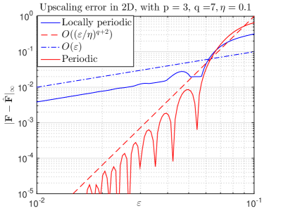
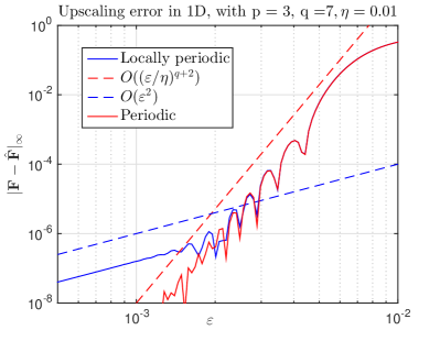
The left plot in Figure 1 shows the O((ε/η)q+2)𝑂superscript𝜀𝜂𝑞2O((\varepsilon/\eta)^{q+2}) convergence rate in (10), for the periodic coefficient given in (11), and O(ε2)𝑂superscript𝜀2O(\varepsilon^{2}) asymptotic rate for the locally-periodic coefficient. Consider also the two-dimensional coefficients

A(𝐲)𝐴𝐲\displaystyle A({\bf y}) =(1.5+sin(2πy1))(1.5+sin(2πy2)),absent1.52𝜋subscript𝑦11.52𝜋subscript𝑦2\displaystyle=(1.5+\sin(2\pi y_{1}))(1.5+\sin(2\pi y_{2})),
(12) A(𝐱,𝐲)𝐴𝐱𝐲\displaystyle A({\bf x},{\bf y}) =(1.5+sin(2πy1)+sin(2πx2)cos(2πy1)).absent1.52𝜋subscript𝑦12𝜋subscript𝑥22𝜋subscript𝑦1\displaystyle=(1.5+\sin(2\pi y_{1})+\sin(2\pi x_{2})\cos(2\pi y_{1})).

The right plot in Figure 1, depicts the O((ε/η)q+2)𝑂superscript𝜀𝜂𝑞2O((\varepsilon/\eta)^{q+2}) convergence rate that the periodic theory predicts, while an O(ε)𝑂𝜀O(\varepsilon) asymptotic convergence rate is observed for the locally-periodic coefficient in (12).
Refer to caption
Refer to caption
Figure 1. The upscaling errors |𝐅𝐅^|subscript𝐅^𝐅|{\bf F}-\hat{{\bf F}}|_{\infty} for periodic and locally-periodic materials in one and two dimensions are depicted. (Left) Upscaling error for the periodic and locally-periodic coefficients (11) in one dimension: the micro problem (14) is solved with the parameters τ=η=0.01𝜏𝜂0.01\tau=\eta=0.01. The result indicates different convergence rates in periodic and locally-periodic media. (Right) Upscaling error for the periodic and locally-periodic coefficients (11) in two dimensions: the micro problem (14) is solved with the parameters τ=η=0.1𝜏𝜂0.1\tau=\eta=0.1. The result indicates again different convergence rates in periodic and locally-periodic media. Note also the dependency of the convergence rates, in locally-periodic media, on the dimension. In one dimension, we observe O(ε2)𝑂superscript𝜀2O(\varepsilon^{2}) asymptotic rate while in two dimensions the convergence rate becomes O(ε)𝑂𝜀O(\varepsilon).

In the present paper, we are able to give a rigorous analysis revealing the convergence rates in a multi-dimensional locally-periodic setting. Moreover, our theory fully explains the mentioned dimension-dependent phenomenon. The main result of this paper is the following theorem.

Theorem 1.

Let 𝐅𝐅{\bf F} be given as in (15), and 𝐅^^𝐅\hat{{\bf F}} be the homogenized flux (9). Furthermore, let u^=𝐬𝐱^𝑢𝐬𝐱\hat{u}={\bf s}\cdot{\bf x}, K𝕂p,q𝐾superscript𝕂𝑝𝑞K\in\mathbb{K}^{p,q} with an even q𝑞q and p>1𝑝1p>1, and 0<εη=τ<10𝜀𝜂𝜏10<\varepsilon\leq\eta=\tau<1, and assume that 𝐫0subscript𝐫0{\bf r}_{0} belongs to the compact set Ω¯¯Ω\overline{\Omega}. Then

sup𝐫0Ω¯|𝐅(𝐫0)𝐅^(𝐫0)|C|𝐬|{(εη)q1+ε5η7,d=1,(εη)q1+ε+ε5η7,d>1.subscriptsupremumsubscript𝐫0¯Ωsubscript𝐅subscript𝐫0^𝐅subscript𝐫0𝐶subscript𝐬casessuperscript𝜀𝜂𝑞1superscript𝜀5superscript𝜂7𝑑1superscript𝜀𝜂𝑞1𝜀superscript𝜀5superscript𝜂7𝑑1\displaystyle\sup_{{\bf r}_{0}\in\overline{\Omega}}\left|{\bf F}({\bf r}_{0})-\hat{{\bf F}}({\bf r}_{0})\right|_{\infty}\leq C\left|{\bf s}\right|_{\infty}\begin{cases}\left(\dfrac{\varepsilon}{\eta}\right)^{q-1}+\varepsilon^{-5}\eta^{7},&d=1,\\ \left(\dfrac{\varepsilon}{\eta}\right)^{q-1}+\varepsilon+\varepsilon^{-5}\eta^{7},&d>1.\end{cases}

where C𝐶C does not depend on 𝐱,ε,η𝐱𝜀𝜂{\bf x},\varepsilon,\eta but may depend on K,p,q,d𝐾𝑝𝑞𝑑K,p,q,d or A𝐴A. Moreover, if η=ε1β𝜂superscript𝜀1𝛽\eta=\varepsilon^{1-\beta} for 0<β<2/70𝛽270<\beta<2/7, then

(13) sup𝐫0Ω¯|𝐅(𝐫0)𝐅^(𝐫0)|C|𝐬|{εβ(q1)+ε27βd=1,εβ(q1)+ε+ε27βd>1.subscriptsupremumsubscript𝐫0¯Ωsubscript𝐅subscript𝐫0^𝐅subscript𝐫0𝐶subscript𝐬casessuperscript𝜀𝛽𝑞1superscript𝜀27𝛽𝑑1superscript𝜀𝛽𝑞1𝜀superscript𝜀27𝛽𝑑1\displaystyle\sup_{{\bf r}_{0}\in\overline{\Omega}}\left|{\bf F}({\bf r}_{0})-\hat{{\bf F}}({\bf r}_{0})\right|_{\infty}\leq C|{\bf s}|_{\infty}\begin{cases}\varepsilon^{\beta\left(q-1\right)}+\varepsilon^{2-7\beta}&d=1,\\ \varepsilon^{\beta\left(q-1\right)}+\varepsilon+\varepsilon^{2-7\beta}&d>1.\end{cases}
Remark 5.

The HMM error in (13) can be made almost equal to O(εk+ε2)𝑂superscript𝜀𝑘superscript𝜀2O(\varepsilon^{k}+\varepsilon^{2}) for d=1𝑑1d=1 and to O(εk+ε)𝑂superscript𝜀𝑘𝜀O(\varepsilon^{k}+\varepsilon) for d>1𝑑1d>1, where k2𝑘2k\geq 2, upon choosing small enough β𝛽\beta and a large enough q𝑞q, i.e., q=k/β+1𝑞𝑘𝛽1q=k/\beta+1. Small values for the parameter β𝛽\beta imply a low computational cost as the size of the micro domains are η=O(ε1β)O(ε)𝜂𝑂superscript𝜀1𝛽𝑂𝜀\eta=O(\varepsilon^{1-\beta})\approx O(\varepsilon).

Remark 6.

Note that the simulations in Figure 1 are done for fixed η𝜂\eta and varying ε𝜀\varepsilon, and that O(ε2)𝑂superscript𝜀2O(\varepsilon^{2}) and O(ε)𝑂𝜀O(\varepsilon) asymptotic rates are observed in one and two dimensions respectively. Theorem 1, however, suggests an O(ε5)𝑂superscript𝜀5O(\varepsilon^{-5}) asymptotic error which is not seen in the Figure. This is due to the fact that the error bound in Theorem 1 is not sharp. But note that the right asymptotic rates are recovered upon choosing η=ε1β𝜂superscript𝜀1𝛽\eta=\varepsilon^{1-\beta}.

4. Analysis

4.1. Simplifications

We start by some simplifications for the analysis. Let 𝐫0subscript𝐫0{\bf r}_{0} represent a fixed but arbitrary point in the domain ΩΩ\Omega. We consider the micro-problem (7), centred at 𝐫0subscript𝐫0{\bf r}_{0} (Ω𝐫0,η=𝐫0+[Lη,Lη]dsubscriptΩsubscript𝐫0𝜂subscript𝐫0superscriptsubscript𝐿𝜂subscript𝐿𝜂𝑑\Omega_{{\bf r}_{0},\eta}={\bf r}_{0}+{\color[rgb]{0,0,0}[-L_{\eta},L_{\eta}]^{d}}), with initial data

u^(𝐱)=𝐬(𝐱𝐫0),^𝑢𝐱𝐬𝐱subscript𝐫0\hat{u}({\bf x})={\bf s}\cdot({\bf x}-{\bf r}_{0}),

where 𝐬=u^(𝐫0)d𝐬^𝑢subscript𝐫0superscript𝑑{\bf s}=\nabla\hat{u}{\color[rgb]{0,0,0}({\bf r}_{0})}\in\mathbb{R}^{d} is the slope vector. Note that the constant term c0subscript𝑐0c_{0} introduced in Section 2 is removed from the notation as constant initial data would have zero contribution to the flux. The starting point of the analysis is to set the local problem (7) on dsuperscript𝑑\mathbb{R}^{d} and (without loss of generality) shift the micro problem to the origin.

(14) ttuε,η(t,𝐱)subscript𝑡𝑡superscript𝑢𝜀𝜂𝑡𝐱\displaystyle\partial_{tt}u^{\varepsilon,\eta}(t,{\bf x}) =(A(𝐱+𝐫0,(𝐱+𝐫0)/ε)uε,η(t,𝐱)), in d×(0,τ/2],absent𝐴𝐱subscript𝐫0𝐱subscript𝐫0𝜀superscript𝑢𝜀𝜂𝑡𝐱 in superscript𝑑0𝜏2\displaystyle=\nabla\cdot\left(A({\bf x}+{\bf r}_{0},({\bf x}+{\bf r}_{0})/\varepsilon)\nabla u^{\varepsilon,\eta}(t,{\bf x})\right),\text{ in }\mathbb{R}^{d}\times(0,\tau/2],
uε,η(0,𝐱)superscript𝑢𝜀𝜂0𝐱\displaystyle u^{\varepsilon,\eta}(0,{\bf x}) =𝐬𝐱,tuε,η(0,𝐱)=0.formulae-sequenceabsent𝐬𝐱subscript𝑡superscript𝑢𝜀𝜂0𝐱0\displaystyle={\bf s}\cdot{\bf x},\quad\partial_{t}u^{\varepsilon,\eta}(0,{\bf x})=0.

Posing the micro-problem (14) over dsuperscript𝑑\mathbb{R}^{d} is only to simplify the analysis, and does not affect the computational results. This is due to the finite speed of propagation of waves; namely the solution (of the local mixed initial-boundary value problem (7)) in the interior region [0,τ/2]×[η/2,η/2]d0𝜏2superscript𝜂2𝜂2𝑑[0,\tau/2]\times[-\eta/2,\eta/2]^{d}, which is needed in the upscaling step (8), will be the same as the solution of the corresponding Cauchy problem (14) since the interior solution will not be influenced by the periodic conditions of the local problem (7) if Lηη/2+τ/2|A|subscript𝐿𝜂𝜂2𝜏2subscript𝐴L_{\eta}\geq\eta/2+\tau/2\sqrt{|A|_{\infty}}, see [9] for more discussions and numerical results. Moreover, we rewrite the flux (8) as

(15) 𝐅(𝐫0)=ττΩ0,ηKη(𝐱)Kτ(t)A(𝐱+𝐫0,𝐱/ε+𝐫0/ε)uε,η(t,𝐱)𝑑𝐱𝑑t.𝐅subscript𝐫0superscriptsubscript𝜏𝜏subscriptsubscriptΩ0𝜂subscript𝐾𝜂𝐱subscript𝐾𝜏𝑡𝐴𝐱subscript𝐫0𝐱𝜀subscript𝐫0𝜀superscript𝑢𝜀𝜂𝑡𝐱differential-d𝐱differential-d𝑡{\bf F}({\bf r}_{0})=\int_{-\tau}^{\tau}\int_{\Omega_{0,\eta}}K_{\eta}({\bf x})K_{\tau}(t)A({\bf x}+{\bf r}_{0},{\bf x}/\varepsilon+{\bf r}_{0}/\varepsilon)\nabla u^{\varepsilon,\eta}(t,{\bf x})\;d{\bf x}\;dt.

We introduce also

A𝐫0,γ(𝐱,𝐱/ε):=A(𝐱+𝐫0,𝐱/ε+γ).assignsubscript𝐴subscript𝐫0𝛾𝐱𝐱𝜀𝐴𝐱subscript𝐫0𝐱𝜀𝛾A_{{\bf r}_{0},\gamma}({\bf x},{\bf x}/\varepsilon):=A({\bf x}+{\bf r}_{0},{\bf x}/\varepsilon+\gamma).

As A𝐴A is periodic in the second argument, we can replace the coefficient A𝐴A in (14) by A𝐫0,γsubscript𝐴subscript𝐫0𝛾A_{{\bf r}_{0},\gamma} evaluated at γ={𝐫0/ε}𝛾subscript𝐫0𝜀\gamma=\{{\bf r}_{0}/\varepsilon\}, where {𝐚}𝐚\{{\bf a}\} denotes the fractional part of 𝐚d𝐚superscript𝑑{\bf a}\in\mathbb{R}^{d}.

4.2. Outline of the analysis

  • Step 1.

    Expansion: In this part, the solution is scaled as uε,η(t,𝐱)=εv(t/ε,𝐱/ε)superscript𝑢𝜀𝜂𝑡𝐱𝜀𝑣𝑡𝜀𝐱𝜀u^{\varepsilon,\eta}(t,{\bf x})=\varepsilon v(t/\varepsilon,{\bf x}/\varepsilon), and an asymptotic expansion is used to express v𝑣v as

    v(t,𝐱)v0(t,𝐱)+εv1(t,𝐱)+ε22v2(t,𝐱)+.𝑣𝑡𝐱subscript𝑣0𝑡𝐱𝜀subscript𝑣1𝑡𝐱superscript𝜀22subscript𝑣2𝑡𝐱v(t,{\bf x})\approx v_{0}(t,{\bf x})+\varepsilon v_{1}(t,{\bf x})+\dfrac{\varepsilon^{2}}{2}v_{2}(t,{\bf x})+\ldots.

    The main result of the section is to estimate the difference between u~1ε,η:=εv0(t/ε,𝐱/ε)+ε2v1(t/ε,𝐱/ε)assignsuperscriptsubscript~𝑢1𝜀𝜂𝜀subscript𝑣0𝑡𝜀𝐱𝜀superscript𝜀2subscript𝑣1𝑡𝜀𝐱𝜀\tilde{u}_{1}^{\varepsilon,\eta}:=\varepsilon v_{0}(t/\varepsilon,{\bf x}/\varepsilon)+\varepsilon^{2}v_{1}(t/\varepsilon,{\bf x}/\varepsilon), and uε,ηsuperscript𝑢𝜀𝜂u^{\varepsilon,\eta} the solution of the micro problem (14).

  • Step 2.

    Quasi-polynomials: The main aim in this part is to write v0(t,𝐱)subscript𝑣0𝑡𝐱v_{0}(t,{\bf x}) and v1(t,𝐱)subscript𝑣1𝑡𝐱v_{1}(t,{\bf x}) in terms of simpler (periodic) functions. Namely, we show that

    v0(t,𝐲)=𝐬𝐲+v00(t,𝐲), and v1(t,𝐲)=v10(t,𝐲)+j=1dyjv11j(t,𝐲),formulae-sequencesubscript𝑣0𝑡𝐲𝐬𝐲subscript𝑣00𝑡𝐲 and subscript𝑣1𝑡𝐲subscript𝑣10𝑡𝐲superscriptsubscript𝑗1𝑑subscript𝑦𝑗subscript𝑣11𝑗𝑡𝐲v_{0}(t,{\bf y})={\bf s}\cdot{\bf y}+v_{00}(t,{\bf y}),\text{ and }v_{1}(t,{\bf y})=v_{10}(t,{\bf y})+\sum_{j=1}^{d}y_{j}v_{11j}(t,{\bf y}),

    where v00(t,),v10(t,),{v11j(t,)}j=1dsubscript𝑣00𝑡subscript𝑣10𝑡superscriptsubscriptsubscript𝑣11𝑗𝑡𝑗1𝑑v_{00}(t,\cdot),v_{10}(t,\cdot),\{v_{11j}(t,\cdot)\}_{j=1}^{d} are periodic functions on Y:=(0,1]dassign𝑌superscript01𝑑Y:=(0,1]^{d}.

  • Step 3.

    Energy estimates: This part includes energy estimates for elliptic and second order hyperbolic PDEs. The results of this section is used later in Step 4.

  • Step 4.

    Time averages: In the upscaling step (8), the averaging operator in time can be treated separately from the spatial averaging operator due to linearity, see Subsection 4.6. The main aim is to write down explicit equations for the temporally averaged quantities defined by d00(𝐲):=Kτv00(/ε,𝐲)d_{00}({\bf y}):=K_{\tau}\ast v_{00}(\cdot/\varepsilon,{\bf y}), and for d11jsubscript𝑑11𝑗d_{11j}, and d10subscript𝑑10d_{10} (which are defined similarly).

  • Step 5.

    Decomposition of the flux: In this part, the HMM flux (8) is decomposed as

    𝐅(𝐫0)𝐅subscript𝐫0\displaystyle{\bf F}({\bf r}_{0}) =(𝒦τ,ηA(,/ε)u~ε,η(,))(0,0)+(𝒦τ,ηA(,/ε)(uε,ηu~1ε,η))(0,0)tail,\displaystyle=\left(\mathcal{K}_{\tau,\eta}\ast A(\cdot,\cdot/\varepsilon)\nabla\tilde{u}^{\varepsilon,\eta}(\cdot,\cdot)\right)(0,0)+\underbrace{\left(\mathcal{K}_{\tau,\eta}\ast A(\cdot,\cdot/\varepsilon)\left(\nabla u^{\varepsilon,\eta}-\nabla\tilde{u}_{1}^{\varepsilon,\eta}\right)\right)(0,0)}_{\mathcal{E}_{tail}},

    and the HMM flux is expressed as 𝐅=𝐅0+ε𝐅1+δ+tail𝐅subscript𝐅0𝜀subscript𝐅1𝛿subscript𝑡𝑎𝑖𝑙{\bf F}={\bf F}_{0}+\varepsilon{\bf F}_{1}+\delta+\mathcal{E}_{tail}, where

    𝐅0(𝐫0)subscript𝐅0subscript𝐫0\displaystyle{\bf F}_{0}({\bf r}_{0}) =(KηA(,/ε)(𝐬+𝐲d00(/ε)))(0)\displaystyle=\left(K_{\eta}\ast A(\cdot,\cdot/\varepsilon)\left({\bf s}+\nabla_{\bf y}d_{00}(\cdot/\varepsilon)\right)\right)(0)
    𝐅1(𝐫0)subscript𝐅1subscript𝐫0\displaystyle{\bf F}_{1}({\bf r}_{0}) =(KηA(,/ε)(𝐲d10(/ε)+d11(/ε)))(0)\displaystyle=\left(K_{\eta}\ast A(\cdot,\cdot/\varepsilon)\left(\nabla_{\bf y}d_{10}(\cdot/\varepsilon)+d_{11}(\cdot/\varepsilon)\right)\right)(0)
    δ(𝐫0)𝛿subscript𝐫0\displaystyle\delta({\bf r}_{0}) =(Kηj=1dxjA(,/ε)𝐲d11j(/ε))(0).\displaystyle=\left(K_{\eta}\ast\sum_{j=1}^{d}x_{j}A(\cdot,\cdot/\varepsilon)\nabla_{\bf y}d_{11j}(\cdot/\varepsilon)\right)(0).

    Moreover, the result from Step 2 is used to estimate the tail tailsubscript𝑡𝑎𝑖𝑙\mathcal{E}_{tail}.

  • Step 6.

    The main proof: Here it is proved that |𝐅𝐅0|C(ε/η)q𝐅subscript𝐅0𝐶superscript𝜀𝜂𝑞|{\bf F}-{\bf F}_{0}|\leq C(\varepsilon/\eta)^{q}, and that the terms ε𝐅1𝜀subscript𝐅1\varepsilon{\bf F}_{1} and δ𝛿\delta are bounded and small, and the final estimate is obtained. It is also proved that in one-dimension the result |𝐅1|C(ε/η)q1subscript𝐅1𝐶superscript𝜀𝜂𝑞1|{\bf F}_{1}|\leq C(\varepsilon/\eta)^{q-1} holds; explaining the one-dimensional effect seen in the numerics.

4.3. Expansion

We consider now the micro problem (14) which is posed over dsuperscript𝑑\mathbb{R}^{d}. By the scaling uε,η(εt,ε𝐱):=εv(t,𝐱;ε,𝐫0,γ)assignsuperscript𝑢𝜀𝜂𝜀𝑡𝜀𝐱𝜀𝑣𝑡𝐱𝜀subscript𝐫0𝛾u^{\varepsilon,\eta}(\varepsilon t,\varepsilon{\bf x}):=\varepsilon v(t,{\bf x};\varepsilon,{\bf r}_{0},\gamma) we have

(16) ttv(t,𝐱;ε,𝐫0,γ)=(A𝐫0,γ(ε𝐱,𝐱)v(t,𝐱;ε,𝐫0,γ)),subscript𝑡𝑡𝑣𝑡𝐱𝜀subscript𝐫0𝛾subscript𝐴subscript𝐫0𝛾𝜀𝐱𝐱𝑣𝑡𝐱𝜀subscript𝐫0𝛾\displaystyle\partial_{tt}v(t,{\bf x};\varepsilon,{\bf r}_{0},\gamma)=\nabla\cdot\left(A_{{\bf r}_{0},\gamma}(\varepsilon{\bf x},{\bf x})\nabla v(t,{\bf x};\varepsilon,{\bf r}_{0},\gamma)\right),
v(0,𝐱;ε,𝐫0,γ)=𝐬𝐱,tv(0,𝐱;ε,𝐫0,γ)=0.formulae-sequence𝑣0𝐱𝜀subscript𝐫0𝛾𝐬𝐱subscript𝑡𝑣0𝐱𝜀subscript𝐫0𝛾0\displaystyle v(0,{\bf x};\varepsilon,{\bf r}_{0},\gamma)={\bf s}\cdot{\bf x},\quad\partial_{t}v(0,{\bf x};\varepsilon,{\bf r}_{0},\gamma)=0.

Now we define vk(t,𝐱;𝐫0,γ):=εkv(t,𝐱;0,𝐫0,γ)assignsubscript𝑣𝑘𝑡𝐱subscript𝐫0𝛾superscriptsubscript𝜀𝑘𝑣𝑡𝐱0subscript𝐫0𝛾v_{k}(t,{\bf x};{\bf r}_{0},\gamma):=\partial_{\varepsilon}^{k}v(t,{\bf x};0,{\bf r}_{0},\gamma), and consider the expansion

(17) v(t,𝐱;ε,𝐫0,γ)=v0(t,𝐱;𝐫0,γ)+εv1(t,𝐱;𝐫0,γ)+ε22v2(t,𝐱;𝐫0,γ)+R(t,𝐱;ε,𝐫0,γ).𝑣𝑡𝐱𝜀subscript𝐫0𝛾subscript𝑣0𝑡𝐱subscript𝐫0𝛾𝜀subscript𝑣1𝑡𝐱subscript𝐫0𝛾superscript𝜀22subscript𝑣2𝑡𝐱subscript𝐫0𝛾𝑅𝑡𝐱𝜀subscript𝐫0𝛾v(t,{\bf x};\varepsilon,{\bf r}_{0},\gamma)=v_{0}(t,{\bf x};{\bf r}_{0},\gamma)+\varepsilon v_{1}(t,{\bf x};{\bf r}_{0},\gamma)+\dfrac{\varepsilon^{2}}{2}v_{2}(t,{\bf x};{\bf r}_{0},\gamma){\color[rgb]{0,0,0}+R(t,{\bf x};\varepsilon,{\bf r}_{0},\gamma).}

For k=0𝑘0k=0, we have

ttv0(t,𝐱;𝐫0,γ)=(A𝐫0,γ(0,𝐱)v0(t,𝐱;𝐫0,γ)),subscript𝑡𝑡subscript𝑣0𝑡𝐱subscript𝐫0𝛾subscript𝐴subscript𝐫0𝛾0𝐱subscript𝑣0𝑡𝐱subscript𝐫0𝛾\displaystyle\partial_{tt}v_{0}(t,{\bf x};{\bf r}_{0},\gamma)=\nabla\cdot\left(A_{{\bf r}_{0},\gamma}(0,{\bf x})\nabla v_{0}(t,{\bf x};{\bf r}_{0},\gamma)\right),
(18) v0(0,𝐱;𝐫0,γ)=𝐬𝐱,tv0(0,𝐱;𝐫0,γ)=0.formulae-sequencesubscript𝑣00𝐱subscript𝐫0𝛾𝐬𝐱subscript𝑡subscript𝑣00𝐱subscript𝐫0𝛾0\displaystyle v_{0}(0,{\bf x};{\bf r}_{0},\gamma)={\bf s}\cdot{\bf x},\quad\partial_{t}v_{0}(0,{\bf x};{\bf r}_{0},\gamma)=0.

Let v0=𝐬𝐱+v00(t,𝐱;𝐫0,γ)subscript𝑣0𝐬𝐱subscript𝑣00𝑡𝐱subscript𝐫0𝛾v_{0}={\bf s}\cdot{\bf x}+v_{00}(t,{\bf x};{\bf r}_{0},\gamma), then

(19) ttv00(t,𝐱;𝐫0,γ)subscript𝑡𝑡subscript𝑣00𝑡𝐱subscript𝐫0𝛾\displaystyle\partial_{tt}v_{00}(t,{\bf x};{\bf r}_{0},\gamma) =(A𝐫0,γ(0,𝐱)v00(t,𝐱;𝐫0,γ))+A𝐫0,γ(0,𝐱)𝐬absentsubscript𝐴subscript𝐫0𝛾0𝐱subscript𝑣00𝑡𝐱subscript𝐫0𝛾subscript𝐴subscript𝐫0𝛾0𝐱𝐬\displaystyle=\nabla\cdot\left(A_{{\bf r}_{0},\gamma}(0,{\bf x})\nabla v_{00}(t,{\bf x};{\bf r}_{0},\gamma)\right)+\nabla\cdot A_{{\bf r}_{0},\gamma}(0,{\bf x}){\bf s}
v00(0,𝐱;𝐫0,γ)subscript𝑣000𝐱subscript𝐫0𝛾\displaystyle v_{00}(0,{\bf x};{\bf r}_{0},\gamma) =tv00(0,𝐱;𝐫0,γ)=0.absentsubscript𝑡subscript𝑣000𝐱subscript𝐫0𝛾0\displaystyle=\partial_{t}v_{00}(0,{\bf x};{\bf r}_{0},\gamma)=0.

For the higher order terms we have the following relation

ttvm(t,𝐱;𝐫0,γ)subscript𝑡𝑡subscript𝑣𝑚𝑡𝐱subscript𝐫0𝛾\displaystyle\partial_{tt}v_{m}(t,{\bf x};{\bf r}_{0},\gamma) =(A𝐫0,γ(0,𝐱)vm(t,𝐱;𝐫0,γ))+Gm(t,𝐱;𝐫0,γ)absentsubscript𝐴subscript𝐫0𝛾0𝐱subscript𝑣𝑚𝑡𝐱subscript𝐫0𝛾subscript𝐺𝑚𝑡𝐱subscript𝐫0𝛾\displaystyle=\nabla\cdot\left(A_{{\bf r}_{0},\gamma}(0,{\bf x})\nabla v_{m}(t,{\bf x};{\bf r}_{0},\gamma)\right)+G_{m}(t,{\bf x};{\bf r}_{0},\gamma)
(20) vm(0,𝐱;𝐫0,γ)subscript𝑣𝑚0𝐱subscript𝐫0𝛾\displaystyle v_{m}(0,{\bf x};{\bf r}_{0},\gamma) =tvm(0,𝐱;𝐫0,γ)=0,m>0,formulae-sequenceabsentsubscript𝑡subscript𝑣𝑚0𝐱subscript𝐫0𝛾0𝑚0\displaystyle=\partial_{t}v_{m}(0,{\bf x};{\bf r}_{0},\gamma)=0,\quad m>0,

where Gmsubscript𝐺𝑚G_{m} is, with cjm=(mj)subscript𝑐𝑗𝑚binomial𝑚𝑗c_{jm}=\dbinom{m}{j},

Gm(t,𝐱;𝐫0,γ)=(j=0m1cjm(εmjA𝐫0,γ(ε𝐱,𝐱))|ε=0vj(t,𝐱;𝐫0,γ)).subscript𝐺𝑚𝑡𝐱subscript𝐫0𝛾evaluated-atsuperscriptsubscript𝑗0𝑚1subscript𝑐𝑗𝑚superscriptsubscript𝜀𝑚𝑗subscript𝐴subscript𝐫0𝛾𝜀𝐱𝐱𝜀0subscript𝑣𝑗𝑡𝐱subscript𝐫0𝛾G_{m}(t,{\bf x};{\bf r}_{0},\gamma)=\nabla\cdot\left(\sum_{j=0}^{m-1}c_{jm}\left(\partial_{\varepsilon}^{m-j}A_{{\bf r}_{0},\gamma}(\varepsilon{\bf x},{\bf x})\right)|_{\varepsilon=0}\nabla v_{j}(t,{\bf x};{\bf r}_{0},\gamma)\right).
Refer to caption
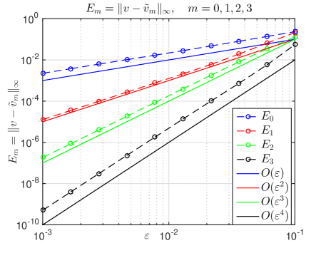
Figure 2. Convergence as ε0𝜀0\varepsilon\longrightarrow 0 of the truncated expansion v~m=k=1mεkk!vksubscript~𝑣𝑚superscriptsubscript𝑘1𝑚superscript𝜀𝑘𝑘subscript𝑣𝑘\tilde{v}_{m}=\sum_{k=1}^{m}\frac{\varepsilon^{k}}{k!}v_{k}. The problem (4.3) is solved for m=0,1,2,3𝑚0123m=0,1,2,3 in one-dimension with A(x,y)=1.1+0.5(sin(2πx)+sin(2πy))𝐴𝑥𝑦1.10.52𝜋𝑥2𝜋𝑦A(x,y)=1.1+0.5(\sin(2\pi x)+\sin(2\pi y)) in the domain (t,x)[0,1]×[3,3]𝑡𝑥0133(t,x)\in[0,1]\times[-3,3] with periodic boundary conditions. The error is defined as Em=max(t,x)[0,1]×[1.5,1.5]|vv~m|subscript𝐸𝑚subscript𝑡𝑥011.51.5𝑣subscript~𝑣𝑚E_{m}=\max_{(t,x)\in[0,1]\times[-1.5,1.5]}|v-\tilde{v}_{m}|.
Remark 7.

We drop 𝐫0subscript𝐫0{\bf r}_{0} and γ𝛾\gamma in the notation for A𝐫0,γ(0,𝐲)subscript𝐴subscript𝐫0𝛾0𝐲A_{{\bf r}_{0},\gamma}(0,{\bf y}), vj(t,𝐲;𝐫0,γ)subscript𝑣𝑗𝑡𝐲subscript𝐫0𝛾v_{j}(t,{\bf y};{\bf r}_{0},\gamma) and vjk(t,𝐲;𝐫0,γ)subscript𝑣𝑗𝑘𝑡𝐲subscript𝐫0𝛾v_{jk}(t,{\bf y};{\bf r}_{0},\gamma) and simply write A(0,𝐲),vj(t,𝐲)𝐴0𝐲subscript𝑣𝑗𝑡𝐲A(0,{\bf y}),v_{j}(t,{\bf y}) and vjk(t,𝐲)subscript𝑣𝑗𝑘𝑡𝐲v_{jk}(t,{\bf y}). Moreover, in addition to the assumptions on A𝐴A given in the introduction, we assume that 𝐫0subscript𝐫0{\bf r}_{0} belongs to the compact set Ω¯¯Ω\overline{\Omega} so that all the constants are uniform in 𝐫0subscript𝐫0{\bf r}_{0}.

Now we present a theorem to estimate the tail of the expansion in (17).

Theorem 2.

Assume that ΩL=[L,L]dsubscriptΩ𝐿superscript𝐿𝐿𝑑\Omega_{L}=[-L,L]^{d}, and that AC(ΩL×Y)𝐴superscript𝐶subscriptΩ𝐿𝑌A\in C^{\infty}(\Omega_{L}\times Y). Let v(t,𝐱;ε)𝑣𝑡𝐱𝜀v(t,{\bf x};\varepsilon) be the solution of (16) and v~m(t,𝐱;ε)subscript~𝑣𝑚𝑡𝐱𝜀\tilde{v}_{m}(t,{\bf x};\varepsilon) be defined by

(21) v~m(t,𝐱;ε)=k=0mεkk!vk(t,𝐱),subscript~𝑣𝑚𝑡𝐱𝜀superscriptsubscript𝑘0𝑚superscript𝜀𝑘𝑘subscript𝑣𝑘𝑡𝐱\tilde{v}_{m}(t,{\bf x};\varepsilon)=\sum_{k=0}^{m}\frac{\varepsilon^{k}}{k!}v_{k}(t,{\bf x}),

where vksubscript𝑣𝑘v_{k} is given by (18) and (4.3) for k=0𝑘0k=0 and k>1𝑘1k>1 respectively. Then for any M>L+t|A|𝑀𝐿𝑡subscript𝐴M>L+t\sqrt{\left|A\right|_{\infty}}

(vv~m)(t,;ε)L2(ΩL)Cεm+1j=0mMmj(1+M)tmax|z|tvj(z,)H2(ΩM),subscriptnorm𝑣subscript~𝑣𝑚𝑡𝜀superscript𝐿2subscriptΩ𝐿absent𝐶superscript𝜀𝑚1superscriptsubscript𝑗0𝑚superscript𝑀𝑚𝑗1𝑀𝑡subscript𝑧𝑡subscriptnormsubscript𝑣𝑗𝑧superscript𝐻2subscriptΩ𝑀\begin{array}[]{ll}\|\nabla\left(v-\tilde{v}_{m}\right)(t,\cdot;\varepsilon)\|_{L^{2}(\Omega_{L})}&\leq\displaystyle C\varepsilon^{m+1}\sum_{j=0}^{m}M^{m-j}\left(1+M\right)t\max_{|z|\leq t}\left\|v_{j}(z,\cdot)\right\|_{H^{2}(\Omega_{M})},\end{array}

where C𝐶C does not depend on t,ε𝑡𝜀t,\varepsilon and M𝑀M but may depend on A,m,d𝐴𝑚𝑑A,m,d. Moreover, for m=1𝑚1m=1, the above estimate gives

(22) (vv~1)(t,;ε)L2(ΩL)Cε2(1+Md/2+1)(1+M2)(1+t4)|𝐬|.subscriptnorm𝑣subscript~𝑣1𝑡𝜀superscript𝐿2subscriptΩ𝐿absent𝐶superscript𝜀21superscript𝑀𝑑211superscript𝑀21superscript𝑡4subscript𝐬\begin{array}[]{ll}\|\nabla\left(v-\tilde{v}_{1}\right)(t,\cdot;\varepsilon)\|_{L^{2}(\Omega_{L})}&\leq C\varepsilon^{2}\left(1+M^{d/2+1}\right)\left(1+M^{2}\right)\left(1+t^{4}\right)\left|{\bf s}\right|_{\infty}.\end{array}
Proof.

See the appendix. ∎

To illustrate the result of Theorem 2, we present a numerical test in Figure 2, which shows the claimed rate of convergence. Note that M𝑀M and the final time t𝑡t are fixed in the simulation.

Corollary 1.

Let uε,η(t,𝐱)superscript𝑢𝜀𝜂𝑡𝐱u^{\varepsilon,\eta}(t,{\bf x}) be the microscopic solution solving (14) and let u~1ε,η(t,𝐱)subscriptsuperscript~𝑢𝜀𝜂1𝑡𝐱\tilde{u}^{\varepsilon,\eta}_{1}(t,{\bf x}) :=εv~1(t/ε,𝐱/ε;ε)assignabsent𝜀subscript~𝑣1𝑡𝜀𝐱𝜀𝜀:=\varepsilon\tilde{v}_{1}(t/\varepsilon,{\bf x}/\varepsilon;\varepsilon), where v~1subscript~𝑣1\tilde{v}_{1} is given by (21) with m=1𝑚1m=1. Moreover, assume that ετ𝜀𝜏\varepsilon\leq\tau and εη𝜀𝜂\varepsilon\leq\eta. Then, with eε,η(t,𝐱):=uε,η(t,𝐱)u~1ε,η(t,𝐱)assignsuperscript𝑒𝜀𝜂𝑡𝐱superscript𝑢𝜀𝜂𝑡𝐱subscriptsuperscript~𝑢𝜀𝜂1𝑡𝐱e^{\varepsilon,\eta}(t,{\bf x}):=u^{\varepsilon,\eta}(t,{\bf x})-\tilde{u}^{\varepsilon,\eta}_{1}(t,{\bf x}), the estimate (22) implies

supt(0,τ]𝐱eε,η(t,)L2(Ωη)Cε2+d/2((ηε)d/2+3(τε)4+(ηε)d/2+7)|𝐬|,subscriptsupremum𝑡0𝜏subscriptnormsubscript𝐱superscript𝑒𝜀𝜂𝑡superscript𝐿2subscriptΩ𝜂absent𝐶superscript𝜀2𝑑2superscript𝜂𝜀𝑑23superscript𝜏𝜀4superscript𝜂𝜀𝑑27subscript𝐬\begin{array}[]{ll}\displaystyle\sup_{t\in(0,\tau]}\|\nabla_{{\bf x}}e^{\varepsilon,\eta}(t,\cdot)\|_{L^{2}(\Omega_{\eta})}&\leq C\varepsilon^{2+d/2}\left(\left(\dfrac{\eta}{\varepsilon}\right)^{d/2+3}\left(\dfrac{\tau}{\varepsilon}\right)^{4}+\left(\dfrac{\eta}{\varepsilon}\right)^{d/2+7}\right)\left|{\bf s}\right|_{\infty},\end{array}

where C𝐶C does not depend on ε,η,τ𝜀𝜂𝜏\varepsilon,\eta,\tau but may depend on A𝐴A and d𝑑d.

Proof.

Let e:=vv~1assign𝑒𝑣subscript~𝑣1e:=v-\tilde{v}_{1} and eε,η=uε,ηu~1εsuperscript𝑒𝜀𝜂superscript𝑢𝜀𝜂subscriptsuperscript~𝑢𝜀1e^{\varepsilon,\eta}=u^{\varepsilon,\eta}-\tilde{u}^{\varepsilon}_{1}, then eε,η(t,𝐱)=εe(t/ε,𝐱/ε;ε)superscript𝑒𝜀𝜂𝑡𝐱𝜀𝑒𝑡𝜀𝐱𝜀𝜀e^{\varepsilon,\eta}(t,{\bf x})=\varepsilon e(t/\varepsilon,{\bf x}/\varepsilon;\varepsilon) and with 𝐲=𝐱/ε𝐲𝐱𝜀{\bf y}={\bf x}/\varepsilon the chain rule gives

eε,η(t,𝐱)=𝐲e(t/ε,𝐱/ε).superscript𝑒𝜀𝜂𝑡𝐱subscript𝐲𝑒𝑡𝜀𝐱𝜀\nabla e^{\varepsilon,\eta}(t,{\bf x})=\nabla_{\bf y}e(t/\varepsilon,{\bf x}/\varepsilon).

Then with α=ε/η𝛼𝜀𝜂\alpha=\varepsilon/\eta we get

supt(0,τ]eε,ηL2(Ωη)2subscriptsupremum𝑡0𝜏superscriptsubscriptnormsuperscript𝑒𝜀𝜂superscript𝐿2subscriptΩ𝜂2\displaystyle\sup_{t\in\left(0,\tau\right]}\|\nabla e^{\varepsilon,\eta}\|_{L^{2}(\Omega_{\eta})}^{2} =supt(0,τ]Ωη|eε,η(t,𝐱)|2𝑑𝐱=supt(0,τ]Ωη|𝐲e(t/ε,𝐱/ε)|2𝑑𝐱absentsubscriptsupremum𝑡0𝜏subscriptsubscriptΩ𝜂superscriptsuperscript𝑒𝜀𝜂𝑡𝐱2differential-d𝐱subscriptsupremum𝑡0𝜏subscriptsubscriptΩ𝜂superscriptsubscript𝐲𝑒𝑡𝜀𝐱𝜀2differential-d𝐱\displaystyle=\sup_{t\in\left(0,\tau\right]}\int_{\Omega_{\eta}}\left|\nabla e^{\varepsilon,\eta}(t,{\bf x})\right|^{2}d{\bf x}=\sup_{t\in\left(0,\tau\right]}\int_{\Omega_{\eta}}\left|\nabla_{\bf y}e(t/\varepsilon,{\bf x}/\varepsilon)\right|^{2}d{\bf x}
=εdsupt(0,τ]Ωα1|𝐲e(t/ε,𝐲)|2𝑑𝐲=εdsupt(0,τ/ε]𝐲e(t,)L2(Ωα1)2.absentsuperscript𝜀𝑑subscriptsupremum𝑡0𝜏subscriptsubscriptΩsuperscript𝛼1superscriptsubscript𝐲𝑒𝑡𝜀𝐲2differential-d𝐲superscript𝜀𝑑subscriptsupremum𝑡0𝜏𝜀superscriptsubscriptnormsubscript𝐲𝑒𝑡superscript𝐿2subscriptΩsuperscript𝛼12\displaystyle=\varepsilon^{d}\sup_{t\in\left(0,\tau\right]}\int_{\Omega_{\alpha^{-1}}}\left|\nabla_{\bf y}e(t/\varepsilon,{\bf y})\right|^{2}d{\bf y}=\varepsilon^{d}{\color[rgb]{0,0,0}\sup_{t\in\left(0,\tau/\varepsilon\right]}\left\|\nabla_{{\bf y}}e(t,\cdot)\right\|_{L^{2}(\Omega_{\alpha^{-1}})}^{2}.}

The final result follows by exploiting the last inequality and by putting t=τ/ε𝑡𝜏𝜀t=\tau/\varepsilon and M=α1𝑀superscript𝛼1M=\alpha^{-1} in estimate (22). ∎

4.4. Quasi-polynomials

From an analysis point of view it is desirable to deal with purely periodic functions. Unfortunately, the terms vmsubscript𝑣𝑚v_{m} in (4.3) are not periodic. However, they possess a nice structure known as the quasi-polynomials where the coefficients of usual polynomials are replaced by Y𝑌Y-periodic smooth functions.

Definition 1.

A function P(𝐱,𝐲):𝕕×𝕕:𝑃𝐱𝐲superscript𝕕superscript𝕕P({\bf x},{\bf y}):\mathbb{R^{d}\times\mathbb{R}^{d}\longrightarrow\mathbb{R}} belongs to the set nsubscript𝑛\mathbb{P}_{n} of quasi-polynomials of degree n𝑛n if

P(𝐱,𝐲)=|β|npβ(𝐲)𝐱β,𝑃𝐱𝐲subscript𝛽𝑛subscript𝑝𝛽𝐲superscript𝐱𝛽P({\bf x},{\bf y})=\sum_{|\beta|\leq n}p_{\beta}({\bf y}){\bf x}^{\beta},

where β𝛽\beta represents a multi-index so that 𝐱β=x1β1x2β2xdβdsuperscript𝐱𝛽superscriptsubscript𝑥1subscript𝛽1superscriptsubscript𝑥2subscript𝛽2superscriptsubscript𝑥𝑑subscript𝛽𝑑{\bf x}^{\beta}=x_{1}^{\beta_{1}}x_{2}^{\beta_{2}}\cdots x_{d}^{\beta_{d}}, |β|=j=1dβj𝛽superscriptsubscript𝑗1𝑑subscript𝛽𝑗|\beta|=\sum_{j=1}^{d}\beta_{j}, and PβC(Y)subscript𝑃𝛽superscript𝐶𝑌P_{\beta}\in C^{\infty}(Y) are infinitely differentiable 111-periodic functions, named the coefficient functions of P𝑃P.

Now we will state a lemma which shows that, in general, periodic wave equations with quasi-polynomial data have quasi-polynomial solutions. For this let us define Q,Z,F(t,,)n𝑄𝑍𝐹𝑡subscript𝑛Q,Z,F(t,\cdot,\cdot)\in\mathbb{P}_{n} so that

Q(𝐱,𝐲)=|β|nqβ(𝐲)𝐱β,Z(𝐱,𝐲)=|β|nzβ(𝐲)𝐱β,F(t,𝐱,𝐲)=|β|nfβ(t,𝐲)𝐱β,formulae-sequence𝑄𝐱𝐲subscript𝛽𝑛subscript𝑞𝛽𝐲superscript𝐱𝛽formulae-sequence𝑍𝐱𝐲subscript𝛽𝑛subscript𝑧𝛽𝐲superscript𝐱𝛽𝐹𝑡𝐱𝐲subscript𝛽𝑛subscript𝑓𝛽𝑡𝐲superscript𝐱𝛽Q({\bf x},{\bf y})=\sum_{|\beta|\leq n}q_{\beta}({\bf y}){\bf x}^{\beta},\quad Z({\bf x},{\bf y})=\sum_{|\beta|\leq n}z_{\beta}({\bf y}){\bf x}^{\beta},\quad F(t,{\bf x},{\bf y})=\sum_{|\beta|\leq n}f_{\beta}(t,{\bf y}){\bf x}^{\beta},

and consider the wave equation with a uniformly elliptic and bounded periodic coefficient BC(Y)𝐵superscript𝐶𝑌B\in C^{\infty}(Y):

ttu=(B(𝐱)u(t,𝐱))+F(t,𝐱,𝐱)subscript𝑡𝑡𝑢𝐵𝐱𝑢𝑡𝐱𝐹𝑡𝐱𝐱\displaystyle\partial_{tt}u=\nabla\cdot\left(B({\bf x})\nabla u(t,{\bf x})\right)+F(t,{\bf x},{\bf x})
(23) u(0,𝐱)=Q(𝐱,𝐱),tu(0,𝐱)=Z(𝐱,𝐱).formulae-sequence𝑢0𝐱𝑄𝐱𝐱subscript𝑡𝑢0𝐱𝑍𝐱𝐱\displaystyle u(0,{\bf x})=Q({\bf x},{\bf x}),\quad\partial_{t}u(0,{\bf x})=Z({\bf x},{\bf x}).

Note that the solution u𝑢u is not bounded in usual H1superscript𝐻1H^{1} spaces (not a weak solution). However, it is a classical solution since it satisfies the wave equation pointwise everywhere. The following lemma states that the solution u𝑢u is a quasi-polynomial of degree n𝑛n as well.

Lemma 1.

There is a family of quasi-polynomials U(t,,)n𝑈𝑡subscript𝑛U(t,\cdot,\cdot)\in\mathbb{P}_{n} such that the solution to (4.4) is given as u(t,𝐱)=U(t,𝐱,𝐱)=|β|nuβ(t,𝐱)𝐱β𝑢𝑡𝐱𝑈𝑡𝐱𝐱subscript𝛽𝑛subscript𝑢𝛽𝑡𝐱superscript𝐱𝛽u(t,{\bf x})=U(t,{\bf x},{\bf x})=\sum_{|\beta|\leq n}u_{\beta}(t,{\bf x}){\bf x}^{\beta}. The coefficient functions of U𝑈U solve the forced periodic wave equations

ttuβ(t,𝐱)=(B(𝐱)uβ(t,𝐱))+pβ+fβsubscript𝑡𝑡subscript𝑢𝛽𝑡𝐱𝐵𝐱subscript𝑢𝛽𝑡𝐱subscript𝑝𝛽subscript𝑓𝛽\displaystyle\partial_{tt}u_{\beta}(t,{\bf x})=\nabla\cdot\left(B({\bf x})\nabla u_{\beta}(t,{\bf x})\right)+p_{\beta}+f_{\beta}
uβ(0,𝐱)=qβ,tuβ(0,𝐱)=zβ,formulae-sequencesubscript𝑢𝛽0𝐱subscript𝑞𝛽subscript𝑡subscript𝑢𝛽0𝐱subscript𝑧𝛽\displaystyle u_{\beta}(0,{\bf x})=q_{\beta},\quad\partial_{t}u_{\beta}(0,{\bf x})=z_{\beta},

where fβ,qβ,zβsubscript𝑓𝛽subscript𝑞𝛽subscript𝑧𝛽f_{\beta},q_{\beta},z_{\beta} are the coefficient functions of F,Q,Z,𝐹𝑄𝑍F,Q,Z, and

pβ(t,𝐱)={0,|β|=n,M[uβ+1],|β|=n1,M[uβ+1]+N[uβ+2],|β|n2,subscript𝑝𝛽𝑡𝐱cases0𝛽𝑛𝑀delimited-[]subscript𝑢𝛽1𝛽𝑛1𝑀delimited-[]subscript𝑢𝛽1𝑁delimited-[]subscript𝑢𝛽2𝛽𝑛2p_{\beta}(t,{\bf x})=\begin{cases}0,&|\beta|=n,\\ M[u_{\beta+1}],&|\beta|=n-1,\\ M[u_{\beta+1}]+N[u_{\beta+2}],&|\beta|\leq n-2,\end{cases}

where (with {ej}j=1dsuperscriptsubscriptsubscript𝑒𝑗𝑗1𝑑\{e_{j}\}_{j=1}^{d} being the standard canonical basis vectors in dsuperscript𝑑\mathbb{R}^{d})

M[uβ+1]𝑀delimited-[]subscript𝑢𝛽1\displaystyle M[u_{\beta+1}] :=j=1d(βj+1)((Bejuβ+ej)+ejTBuβ+ej)assignabsentsuperscriptsubscript𝑗1𝑑subscript𝛽𝑗1𝐵subscript𝑒𝑗subscript𝑢𝛽subscript𝑒𝑗superscriptsubscript𝑒𝑗𝑇𝐵subscript𝑢𝛽subscript𝑒𝑗\displaystyle:=\sum_{j=1}^{d}\left(\beta_{j}+1\right)\left(\nabla\cdot\left(Be_{j}u_{\beta+e_{j}}\right)+e_{j}^{T}B\nabla u_{\beta+e_{j}}\right)
N[uβ+2]𝑁delimited-[]subscript𝑢𝛽2\displaystyle N[u_{\beta+2}] :=i,j=1d(βi+1)(βj+1)eiTBejuβ+ei+ej(1δij)assignabsentsuperscriptsubscript𝑖𝑗1𝑑subscript𝛽𝑖1subscript𝛽𝑗1superscriptsubscript𝑒𝑖𝑇𝐵subscript𝑒𝑗subscript𝑢𝛽subscript𝑒𝑖subscript𝑒𝑗1subscript𝛿𝑖𝑗\displaystyle:=\sum_{i,j=1}^{d}\left(\beta_{i}+1\right)\left(\beta_{j}+1\right)e_{i}^{T}Be_{j}u_{\beta+e_{i}+e_{j}}\left(1-\delta_{ij}\right)
+i=1d(βi+1)(βi+2)eiTBeiuβ+2ei.superscriptsubscript𝑖1𝑑subscript𝛽𝑖1subscript𝛽𝑖2superscriptsubscript𝑒𝑖𝑇𝐵subscript𝑒𝑖subscript𝑢𝛽2subscript𝑒𝑖\displaystyle+\sum_{i=1}^{d}\left(\beta_{i}+1\right)\left(\beta_{i}+2\right)e_{i}^{T}Be_{i}u_{\beta+2e_{i}}.
Proof.

The proof of this Lemma in one-dimension was given in [9]. Here, we give the general proof. Let L=:BL=:\nabla\cdot B\nabla. We first note that

L[wβ(𝐱)𝐱β]=i,j=1dxi(Bij(𝐱)𝐱βxjwβ(x))+i,j=1dβjxi(𝐱βejBij(𝐱)wβ(𝐱))=𝐱βi,j=1dxi(Bij(𝐱)xjwβ(𝐱))+i,j=1dβj𝐱βej(Bjixiwβ(𝐱)+xi(Bijwβ(𝐱)))+i,j=1d((1δij)βiβj+δijβi(βj1))𝐱βeiejBijwβ(𝐱).missing-subexpression𝐿delimited-[]subscript𝑤𝛽𝐱superscript𝐱𝛽superscriptsubscript𝑖𝑗1𝑑subscriptsubscript𝑥𝑖subscript𝐵𝑖𝑗𝐱superscript𝐱𝛽subscriptsubscript𝑥𝑗subscript𝑤𝛽𝑥superscriptsubscript𝑖𝑗1𝑑subscript𝛽𝑗subscriptsubscript𝑥𝑖superscript𝐱𝛽subscript𝑒𝑗subscript𝐵𝑖𝑗𝐱subscript𝑤𝛽𝐱missing-subexpressionabsentsuperscript𝐱𝛽superscriptsubscript𝑖𝑗1𝑑subscriptsubscript𝑥𝑖subscript𝐵𝑖𝑗𝐱subscriptsubscript𝑥𝑗subscript𝑤𝛽𝐱superscriptsubscript𝑖𝑗1𝑑subscript𝛽𝑗superscript𝐱𝛽subscript𝑒𝑗subscript𝐵𝑗𝑖subscriptsubscript𝑥𝑖subscript𝑤𝛽𝐱subscriptsubscript𝑥𝑖subscript𝐵𝑖𝑗subscript𝑤𝛽𝐱missing-subexpressionsuperscriptsubscript𝑖𝑗1𝑑1subscript𝛿𝑖𝑗subscript𝛽𝑖subscript𝛽𝑗subscript𝛿𝑖𝑗subscript𝛽𝑖subscript𝛽𝑗1superscript𝐱𝛽subscript𝑒𝑖subscript𝑒𝑗subscript𝐵𝑖𝑗subscript𝑤𝛽𝐱\begin{array}[]{ll}&L[w_{\beta}({\bf x}){\bf x}^{\beta}]=\displaystyle\sum_{i,j=1}^{d}\partial_{x_{i}}\left(B_{ij}({\bf x}){\bf x}^{\beta}\partial_{x_{j}}w_{\beta}(x)\right)+\sum_{i,j=1}^{d}\beta_{j}\partial_{x_{i}}\left({\bf x}^{\beta-e_{j}}B_{ij}({\bf x})w_{\beta}({\bf x})\right)\\ &=\displaystyle{\bf x}^{\beta}\sum_{i,j=1}^{d}\partial_{x_{i}}\left(B_{ij}({\bf x})\partial_{x_{j}}w_{\beta}({\bf x})\right)+\sum_{i,j=1}^{d}\beta_{j}{\bf x}^{\beta-e_{j}}\left(B_{ji}\partial_{x_{i}}w_{\beta}({\bf x})+\partial_{x_{i}}\left(B_{ij}w_{\beta}({\bf x})\right)\right)\\ &+\displaystyle\sum_{i,j=1}^{d}\left(\left(1-\delta_{ij}\right)\beta_{i}\beta_{j}+\delta_{ij}\beta_{i}\left(\beta_{j}-1\right)\right){\bf x}^{\beta-e_{i}-e_{j}}B_{ij}w_{\beta}({\bf x}).\end{array}

From this it follows that

L[U(t,𝐱,𝐱)]=|β|n𝐱βL[uβ]+|β|ni,j=1dβj𝐱βej(Bjixiuβ+xi(Bijuβ))+|β|ni,j=1d((1δij)βiβj+δijβi(βj1))𝐱βeiejBijuβ=|β|n𝐱βL[uβ]+|β|n1𝐱βj=1d(βj+1)i=1d(Bjixiuβ+ej+xi(Bijuβ+ej))+|β|n2𝐱βi,j=1d((1δij)(βi+1)(βj+1)+δij(βi+2)(βi+1))Bijuβ+ei+ej=|β|n𝐱βL[uβ]+|β|n1xβM[uβ+1]+|β|n2𝐱βN[uβ+2]=|β|n𝐱β(L[uβ]+pβ).missing-subexpression𝐿delimited-[]𝑈𝑡𝐱𝐱subscript𝛽𝑛superscript𝐱𝛽𝐿delimited-[]subscript𝑢𝛽subscript𝛽𝑛superscriptsubscript𝑖𝑗1𝑑subscript𝛽𝑗superscript𝐱𝛽subscript𝑒𝑗subscript𝐵𝑗𝑖subscriptsubscript𝑥𝑖subscript𝑢𝛽subscriptsubscript𝑥𝑖subscript𝐵𝑖𝑗subscript𝑢𝛽missing-subexpressionsubscript𝛽𝑛superscriptsubscript𝑖𝑗1𝑑1subscript𝛿𝑖𝑗subscript𝛽𝑖subscript𝛽𝑗subscript𝛿𝑖𝑗subscript𝛽𝑖subscript𝛽𝑗1superscript𝐱𝛽subscript𝑒𝑖subscript𝑒𝑗subscript𝐵𝑖𝑗subscript𝑢𝛽missing-subexpressionabsentsubscript𝛽𝑛superscript𝐱𝛽𝐿delimited-[]subscript𝑢𝛽subscript𝛽𝑛1superscript𝐱𝛽superscriptsubscript𝑗1𝑑subscript𝛽𝑗1superscriptsubscript𝑖1𝑑subscript𝐵𝑗𝑖subscriptsubscript𝑥𝑖subscript𝑢𝛽subscript𝑒𝑗subscriptsubscript𝑥𝑖subscript𝐵𝑖𝑗subscript𝑢𝛽subscript𝑒𝑗missing-subexpressionsubscript𝛽𝑛2superscript𝐱𝛽superscriptsubscript𝑖𝑗1𝑑1subscript𝛿𝑖𝑗subscript𝛽𝑖1subscript𝛽𝑗1subscript𝛿𝑖𝑗subscript𝛽𝑖2subscript𝛽𝑖1subscript𝐵𝑖𝑗subscript𝑢𝛽subscript𝑒𝑖subscript𝑒𝑗missing-subexpressionabsentsubscript𝛽𝑛superscript𝐱𝛽𝐿delimited-[]subscript𝑢𝛽subscript𝛽𝑛1superscript𝑥𝛽𝑀delimited-[]subscript𝑢𝛽1subscript𝛽𝑛2superscript𝐱𝛽𝑁delimited-[]subscript𝑢𝛽2missing-subexpressionabsentsubscript𝛽𝑛superscript𝐱𝛽𝐿delimited-[]subscript𝑢𝛽subscript𝑝𝛽\begin{array}[]{ll}&L[U(t,{\bf x},{\bf x})]=\displaystyle\sum_{|\beta|\leq n}{\bf x}^{\beta}L[u_{\beta}]+\sum_{|\beta|\leq n}\sum_{i,j=1}^{d}\beta_{j}{\bf x}^{\beta-e_{j}}\left(B_{ji}\partial_{x_{i}}u_{\beta}+\partial_{x_{i}}\left(B_{ij}u_{\beta}\right)\right)\\ &+\displaystyle\sum_{|\beta|\leq n}\sum_{i,j=1}^{d}\left(\left(1-\delta_{ij}\right)\beta_{i}\beta_{j}+\delta_{ij}\beta_{i}\left(\beta_{j}-1\right)\right){\bf x}^{\beta-e_{i}-e_{j}}B_{ij}u_{\beta}\\ &=\displaystyle\sum_{|\beta|\leq n}{\bf x}^{\beta}L[u_{\beta}]+\sum_{|\beta|\leq n-1}{\bf x}^{\beta}\sum_{j=1}^{d}\left(\beta_{j}+1\right)\sum_{i=1}^{d}\left(B_{ji}\partial_{x_{i}}u_{\beta+e_{j}}+\partial_{x_{i}}\left(B_{ij}u_{\beta+e_{j}}\right)\right)\\ &+\displaystyle\sum_{|\beta|\leq n-2}{\bf x}^{\beta}\sum_{i,j=1}^{d}\left(\left(1-\delta_{ij}\right)(\beta_{i}+1)(\beta_{j}+1)+\delta_{ij}(\beta_{i}+2)\left(\beta_{i}+1\right)\right)B_{ij}u_{\beta+e_{i}+e_{j}}\\ &=\displaystyle\sum_{|\beta|\leq n}{\bf x}^{\beta}L[u_{\beta}]+\sum_{|\beta|\leq n-1}x^{\beta}M[u_{\beta+1}]+\displaystyle\sum_{|\beta|\leq n-2}{\bf x}^{\beta}N[u_{\beta+2}]\\ &=\displaystyle\sum_{|\beta|\leq n}{\bf x}^{\beta}\left(L[u_{\beta}]+p_{\beta}\right).\end{array}

On the other hand

ttU(t,𝐱,𝐱)=|β|nttuβ𝐱β=|β|n𝐱β(L[uβ]+pβ+fβ)=L[U]+F.subscript𝑡𝑡𝑈𝑡𝐱𝐱subscript𝛽𝑛subscript𝑡𝑡subscript𝑢𝛽superscript𝐱𝛽subscript𝛽𝑛superscript𝐱𝛽𝐿delimited-[]subscript𝑢𝛽subscript𝑝𝛽subscript𝑓𝛽𝐿delimited-[]𝑈𝐹\partial_{tt}U(t,{\bf x},{\bf x})=\sum_{|\beta|\leq n}\partial_{tt}u_{\beta}{\bf x}^{\beta}=\sum_{|\beta|\leq n}{\bf x}^{\beta}(L[u_{\beta}]+p_{\beta}+f_{\beta})=L[U]+F.

Similarly, the initial data agrees and U(t,𝐱,𝐱)𝑈𝑡𝐱𝐱U(t,{\bf x},{\bf x}) is therefore a solution. ∎

We will now use Lemma 1 to express the solutions of (4.3) as quasi-polynomials. When m=1𝑚1m=1, equation (4.3) reads

(24) ttv1(t,𝐲)=L[v1]+j=1d𝐲((yjxjA(0,𝐲))𝐲v0).subscript𝑡𝑡subscript𝑣1𝑡𝐲𝐿delimited-[]subscript𝑣1superscriptsubscript𝑗1𝑑subscript𝐲subscript𝑦𝑗subscriptsubscript𝑥𝑗𝐴0𝐲subscript𝐲subscript𝑣0\partial_{tt}v_{1}(t,{\bf y})=L[v_{1}]+\sum_{j=1}^{d}\nabla_{{\bf y}}\cdot\left(\left(y_{j}\partial_{x_{j}}A(0,{\bf y})\right)\nabla_{{\bf y}}v_{0}\right).

Recall from (18) that v0subscript𝑣0v_{0} solves

ttv0(t,𝐲)=(A(0,𝐲)v0(t,𝐲)),subscript𝑡𝑡subscript𝑣0𝑡𝐲𝐴0𝐲subscript𝑣0𝑡𝐲\displaystyle\partial_{tt}v_{0}(t,{\bf y})=\nabla\cdot\left(A(0,{\bf y})\nabla v_{0}(t,{\bf y})\right),
v0(0,𝐲)=𝐬𝐲,tv0(0,𝐲)=0.formulae-sequencesubscript𝑣00𝐲𝐬𝐲subscript𝑡subscript𝑣00𝐲0\displaystyle v_{0}(0,{\bf y})={\bf s}\cdot{\bf y},\quad\partial_{t}v_{0}(0,{\bf y})=0.

Since 𝐲v00subscript𝐲subscript𝑣0subscript0\nabla_{\bf y}v_{0}\in\mathbb{P}_{0}, the forcing term of equation (24) will be a quasi-polynomial of degree one. Therefore by Lemma 1 we can write

(25) v1(t,𝐲)=v10(t,𝐲)+j=1dyjv11j(t,𝐲),subscript𝑣1𝑡𝐲subscript𝑣10𝑡𝐲superscriptsubscript𝑗1𝑑subscript𝑦𝑗subscript𝑣11𝑗𝑡𝐲v_{1}(t,{\bf y})=v_{10}(t,{\bf y})+\sum_{j=1}^{d}y_{j}v_{11j}(t,{\bf y}),

where v10subscript𝑣10v_{10} and v11jsubscript𝑣11𝑗v_{11j} are periodic in 𝐲𝐲{\bf y}, and

ttv11ksubscript𝑡𝑡subscript𝑣11𝑘\displaystyle\partial_{tt}v_{11k} =L[v11k]+f11k,k=1,,dformulae-sequenceabsent𝐿delimited-[]subscript𝑣11𝑘subscript𝑓11𝑘𝑘1𝑑\displaystyle=L[v_{11k}]+f_{11k},\quad k=1,\ldots,d
(26) ttv10subscript𝑡𝑡subscript𝑣10\displaystyle\partial_{tt}v_{10} =L[v10]+M[v11]+f10,absent𝐿delimited-[]subscript𝑣10𝑀delimited-[]subscript𝑣11subscript𝑓10\displaystyle=L[v_{10}]+M[v_{11}]+f_{10},

with

f11k=𝐲(xkA𝐬)+𝐲((xkA)𝐲v00)subscript𝑓11𝑘subscript𝐲subscriptsubscript𝑥𝑘𝐴𝐬subscript𝐲subscriptsubscript𝑥𝑘𝐴subscript𝐲subscript𝑣00\displaystyle f_{11k}=\nabla_{{\bf y}}\cdot\left(\partial_{x_{k}}A{\bf s}\right)+\nabla_{{\bf y}}\cdot\left(\left(\partial_{x_{k}}A\right)\nabla_{{\bf y}}v_{00}\right) ,f10=𝐱A𝐬+(𝐱A)𝐲v00\displaystyle,\quad f_{10}=\nabla_{{\bf x}}\cdot A{\bf s}+\left(\nabla_{{\bf x}}\cdot A\right)\cdot\nabla_{\bf y}v_{00}
(27) M[v11]=j=1d𝐲(Aejv11j)𝑀delimited-[]subscript𝑣11superscriptsubscript𝑗1𝑑subscript𝐲𝐴subscript𝑒𝑗subscript𝑣11𝑗\displaystyle M[v_{11}]=\sum_{j=1}^{d}\nabla_{\bf y}\cdot\left(Ae_{j}v_{11j}\right) +j=1dejTA𝐲v11j.superscriptsubscript𝑗1𝑑superscriptsubscript𝑒𝑗𝑇𝐴subscript𝐲subscript𝑣11𝑗\displaystyle+\sum_{j=1}^{d}e_{j}^{T}A\nabla_{\bf y}v_{11j}.
Refer to caption
Refer to caption
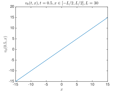
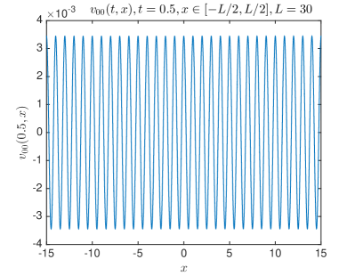
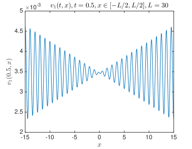
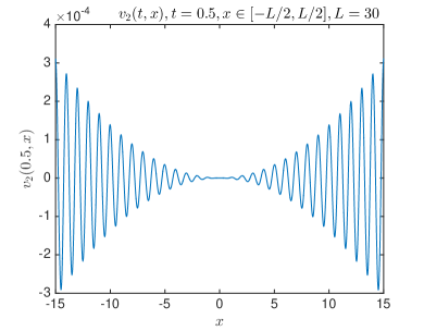
Figure 3. The equation (18) is solved using a one dimensional coefficient A(x,y)=1.1+12(sin(2πx+0.1)+sin(2πy+2))𝐴𝑥𝑦1.1122𝜋𝑥0.12𝜋𝑦2A(x,y)=1.1+\dfrac{1}{2}\left(\sin(2\pi x+0.1)+\sin(2\pi y+2)\right) and the initial data v0(0,x)=xsubscript𝑣00𝑥𝑥v_{0}(0,x)=x over the domain (t,x)(0,1]×[L,L]𝑡𝑥01𝐿𝐿(t,x)\in(0,1]\times[-L,L] for L=30𝐿30L=30. (left) the term v0(t,)subscript𝑣0𝑡v_{0}(t,\cdot) is depicted for t=0.5𝑡0.5t=0.5. (right) the term v00(t,)subscript𝑣00𝑡v_{00}(t,\cdot) is computed by v00=v0xsubscript𝑣00subscript𝑣0𝑥v_{00}=v_{0}-x.
Refer to caption
Refer to caption
Figure 4. The equations (4.3) for m=1𝑚1m=1 and m=2𝑚2m=2 are solved with the same coefficient and domain as in Figure 3. (left) this plot shows that v11subscript𝑣1subscript1v_{1}\in\mathbb{P}_{1} has linear growth in space as the theory of quasi-polynomials predicts. (right) this plot shows that v22subscript𝑣2subscript2v_{2}\in\mathbb{P}_{2} has a quadratic growth in space.
Remark 8.

Using the notation introduced in the beginning of Section 444, the derivative xjA(0,𝐲)subscriptsubscript𝑥𝑗𝐴0𝐲\partial_{x_{j}}A(0,{\bf y}) should be understood as xjA𝐫0,γ(𝐱,𝐲)|𝐱=0evaluated-atsubscriptsubscript𝑥𝑗subscript𝐴subscript𝐫0𝛾𝐱𝐲𝐱0\partial_{x_{j}}A_{{\bf r}_{0},\gamma}({\bf x},{\bf y})|_{{\bf x}=0}.

To illustrate the idea, we present also numerical simulations, in Figures 3 and 4, where we solve (18), and (4.3) for m=1𝑚1m=1 and m=2𝑚2m=2. The numerical results are consistent with the fact that v01subscript𝑣0subscript1v_{0}\in\mathbb{P}_{1}, v11subscript𝑣1subscript1v_{1}\in\mathbb{P}_{1}. Moreover, we observe, in Figure 4, that v22subscript𝑣2subscript2v_{2}\in\mathbb{P}_{2} has a quadratic growth in spatial dimensions.

4.5. Energy estimates

In this section we present energy estimates for elliptic and second order hyperbolic equations. Throughout the section, we will assume Y𝑌Y-periodic uniformly elliptic and bounded coefficients of the form B=B(𝐲)𝐵𝐵𝐲B=B({\bf y}), where BijC(Y¯)subscript𝐵𝑖𝑗superscript𝐶¯𝑌B_{ij}\in C^{\infty}(\overline{Y}). The first lemma concerns the regularity in high order Sobolev norms of solutions to periodic elliptic problems. In this section, we write

L=𝐲B𝐲,𝐿subscript𝐲𝐵subscript𝐲L=\nabla_{\bf y}\cdot B\nabla_{\bf y},

and we denote the averages over the unit cube Y𝑌Y by

f¯:=Yf(𝐲)𝑑𝐲.assign¯𝑓subscript𝑌𝑓𝐲differential-d𝐲\overline{f}:=\int_{Y}f({\bf y})\;d{\bf y}.
Lemma 2.

(Lemma 3.13.13.1 in [9]) Suppose that fHk(Y)𝑓superscript𝐻𝑘𝑌f\in H^{k}(Y) is a Y𝑌Y-periodic function and that f¯=0¯𝑓0\overline{f}=0. Then, for any positive integer n𝑛n, there exists a unique periodic function uHk+2n(Y)𝑢superscript𝐻𝑘2𝑛𝑌u\in H^{k+2n}(Y) satisfying

(1)nLn[u]=f,u¯=0.formulae-sequencesuperscript1𝑛superscript𝐿𝑛delimited-[]𝑢𝑓¯𝑢0(-1)^{n}L^{n}[u]=f,\quad\overline{u}=0.

In addition, the following stability estimate holds

(28) uHk+2n(Y)CfHk(Y),subscriptnorm𝑢superscript𝐻𝑘2𝑛𝑌𝐶subscriptnorm𝑓superscript𝐻𝑘𝑌\displaystyle\|u\|_{H^{k+2n}(Y)}\leq C\|f\|_{H^{k}(Y)},

where C𝐶C does not depend on f𝑓f but may depend on k,Y𝑘𝑌k,Y and B𝐵B.

Now we present a lemma which gives energy estimates for the periodic wave equation in high order Sobolev norms.

Lemma 3.

Let fC([0,T]×Y)𝑓superscript𝐶0𝑇𝑌f\in C^{\infty}([0,T]\times Y), f(t,)𝑓𝑡f(t,\cdot) be Y𝑌Y-periodic, and f(t,)¯=0¯𝑓𝑡0\overline{f(t,\cdot)}=0. Moreover, let g,hC(Y)𝑔superscript𝐶𝑌g,h\in C^{\infty}(Y) be Y𝑌Y-periodic functions with g¯=h¯=0¯𝑔¯0\bar{g}=\bar{h}=0. Then there is a unique solution uC([0,T]×Y)𝑢superscript𝐶0𝑇𝑌u\in C^{\infty}([0,T]\times Y), with u(t,)¯=0¯𝑢𝑡0\overline{u(t,\cdot)}=0, solving

ttu=L[u]+f(t,𝐲),subscript𝑡𝑡𝑢𝐿delimited-[]𝑢𝑓𝑡𝐲\displaystyle\partial_{tt}u=L[u]+f(t,{\bf y}),
u(0,𝐲)=g,tu(0,𝐲)=h.formulae-sequence𝑢0𝐲𝑔subscript𝑡𝑢0𝐲\displaystyle u(0,{\bf y})=g,\quad\partial_{t}u(0,{\bf y})=h.

Moreover, there exists a constant C𝐶C independent of t𝑡t such that for any n0𝑛0n\geq 0

(29) u(t,)H2n+1(Y)CELn[u]1/2(0)+C{0tf(z,)H2n(Y)𝑑z,f is time dependentfH2n(Y),f is time independent,subscriptnorm𝑢𝑡superscript𝐻2𝑛1𝑌𝐶subscriptsuperscript𝐸12superscript𝐿𝑛delimited-[]𝑢0𝐶casessuperscriptsubscript0𝑡subscriptnorm𝑓𝑧superscript𝐻2𝑛𝑌differential-d𝑧𝑓 is time dependentsubscriptnorm𝑓superscript𝐻2𝑛𝑌𝑓 is time independent\|u(t,\cdot)\|_{H^{2n+1}(Y)}\leq CE^{1/2}_{L^{n}[u]}(0)+C\begin{cases}\int_{0}^{t}\|f(z,\cdot)\|_{H^{2n}(Y)}dz,&f\text{ is time dependent}\\ \|f\|_{H^{2n}(Y)},&f\text{ is time independent},\end{cases}

where the energy is defined as

Eu(t):=12Y|tu(t,𝐲)|2+Buu(t,𝐲)d𝐲.assignsubscript𝐸𝑢𝑡12subscript𝑌superscriptsubscript𝑡𝑢𝑡𝐲2𝐵𝑢𝑢𝑡𝐲𝑑𝐲E_{u}(t):=\dfrac{1}{2}\int_{Y}|\partial_{t}u(t,{\bf y})|^{2}+{\color[rgb]{0,0,0}B}\nabla u\cdot\nabla u(t,{\bf y})\;d{\bf y}.
Proof.

The result is classical for n=0𝑛0n=0. To get the estimate for n>0𝑛0n>0, we consider w:=Ln[u]assign𝑤superscript𝐿𝑛delimited-[]𝑢w:=L^{n}[u]. Then by elliptic regularity, Lemma 2, we have

(30) uHk+2n(Y)wHk(Y).subscriptnorm𝑢superscript𝐻𝑘2𝑛𝑌subscriptnorm𝑤superscript𝐻𝑘𝑌\|u\|_{H^{k+2n}(Y)}\leq\|w\|_{H^{k}(Y)}.

Next we apply the operator Lnsuperscript𝐿𝑛L^{n} to the main equation and obtain

ttw(t,y)subscript𝑡𝑡𝑤𝑡𝑦\displaystyle\partial_{tt}w(t,y) =L[w]+Ln[f],absent𝐿delimited-[]𝑤superscript𝐿𝑛delimited-[]𝑓\displaystyle=L[w]+L^{n}[f],
w(0,y)=Ln[g]𝑤0𝑦superscript𝐿𝑛delimited-[]𝑔\displaystyle w(0,y)=L^{n}[g] ,tw(0,𝐲)=Ln[h].\displaystyle,\quad\partial_{t}w(0,{\bf y})=L^{n}[h].

Then we have

w(t,)H1(Y)subscriptnorm𝑤𝑡superscript𝐻1𝑌\displaystyle\|w(t,\cdot)\|_{H^{1}(Y)} CEw1/2(0)+C{0tLn[f](z,)L2(Y)𝑑z,f is time dependentLn[f]L2(Y),f is time independent,absent𝐶subscriptsuperscript𝐸12𝑤0𝐶casessuperscriptsubscript0𝑡subscriptnormsuperscript𝐿𝑛delimited-[]𝑓𝑧superscript𝐿2𝑌differential-d𝑧𝑓 is time dependentsubscriptnormsuperscript𝐿𝑛delimited-[]𝑓superscript𝐿2𝑌𝑓 is time independent\displaystyle\leq CE^{1/2}_{w}(0)+C\begin{cases}\int_{0}^{t}\|L^{n}[f](z,\cdot)\|_{L^{2}(Y)}dz,&f\text{ is time dependent}\\ \|L^{n}[f]\|_{L^{2}(Y)},&f\text{ is time independent},\end{cases}

The final result follows by observing that Ln[f]L2(Y)CfH2n(Y)subscriptnormsuperscript𝐿𝑛delimited-[]𝑓superscript𝐿2𝑌𝐶subscriptnorm𝑓superscript𝐻2𝑛𝑌\|L^{n}[f]\|_{L^{2}(Y)}\leq C\|f\|_{H^{2n}(Y)}, and using the estimate (30) with k=1𝑘1k=1. ∎

4.6. Time averages

The upscaling step in HMM includes averaging of the microscopic flux over micro boxes in time and space, see (15). Since

(Kτuε,η)(t,𝐱)=(Kτuε,η)(t,𝐱),subscript𝐾𝜏superscript𝑢𝜀𝜂𝑡𝐱subscript𝐾𝜏superscript𝑢𝜀𝜂𝑡𝐱\left(K_{\tau}\ast\nabla u^{\varepsilon,\eta}\right)(t,{\bf x})=\nabla\left(K_{\tau}\ast u^{\varepsilon,\eta}\right)(t,{\bf x}),

and since A𝐴A is time independent we can write the HMM flux in (15) as

𝐅(𝐫0)=(KηAε(Kτuε,η))(0,0).𝐅subscript𝐫0subscript𝐾𝜂superscript𝐴𝜀subscript𝐾𝜏superscript𝑢𝜀𝜂00{\bf F}({\bf r}_{0})=\left(K_{\eta}\ast A^{\varepsilon}\nabla\left(K_{\tau}\ast u^{\varepsilon,\eta}\right)\right)(0,0).

The idea is now to write down equations for the time average (Kτuε(,𝐱))(0)subscript𝐾𝜏superscript𝑢𝜀𝐱0\left(K_{\tau}\ast u^{\varepsilon}(\cdot,{\bf x})\right)(0). To do this we start by presenting some intermediate results. First we use a theorem from [9] which is used to derive equations for the local time averages of solutions to periodic wave equations. For the next theorem, we will assume coefficient functions of the form B=B(𝐱,𝐲)𝐵𝐵𝐱𝐲B=B({\bf x},{\bf y}), where BijC(Ω¯×Y¯)subscript𝐵𝑖𝑗superscript𝐶¯Ω¯𝑌B_{ij}\in C^{\infty}(\overline{\Omega}\times\overline{Y}), and B(𝐱,)𝐵𝐱B({\bf x},\cdot) is Y𝑌Y-periodic. We write also L:=𝐲B𝐲assign𝐿subscript𝐲𝐵subscript𝐲L:=\nabla_{\bf y}\cdot B\nabla_{\bf y}.

Theorem 3.

(Theorem 4.14.14.1 in [9]) Suppose α=ετ𝛼𝜀𝜏\alpha=\frac{\varepsilon}{\tau} where 0<ετ0𝜀𝜏0<\varepsilon\leq\tau. Let fC([0,α1],Y)𝑓superscript𝐶0superscript𝛼1𝑌f\in C^{\infty}([0,\alpha^{-1}],Y) be a Y𝑌Y-periodic function with f(t,)¯=0¯𝑓𝑡0\overline{f(t,\cdot)}=0, and K𝕂p,q𝐾superscript𝕂𝑝𝑞K\in\mathbb{K}^{p,q} with an even q𝑞q. Furthermore, assume that w(t,𝐲;𝐱)𝑤𝑡𝐲𝐱w(t,{\bf y};{\bf x}) is the solution of the periodic wave equation parametrized by 𝐱𝐱{\bf x}, i.e., B=B(𝐱,𝐲)𝐵𝐵𝐱𝐲B=B({\bf x},{\bf y}),

(31) ttw(t,𝐲;𝐱)=L[w]+f(t,𝐲;𝐱),w(0,𝐲;𝐱)=tw(0,𝐲;𝐱)=0.subscript𝑡𝑡𝑤𝑡𝐲𝐱𝐿delimited-[]𝑤𝑓𝑡𝐲𝐱missing-subexpression𝑤0𝐲𝐱subscript𝑡𝑤0𝐲𝐱0missing-subexpression\begin{array}[]{ll}\partial_{tt}w(t,{\bf y};{\bf x})=L[w]+f(t,{\bf y};{\bf x}),\\ w(0,{\bf y};{\bf x})=\partial_{t}w(0,{\bf y};{\bf x})=0.\end{array}

Then the local time average d{2k}(𝐱,𝐲):=Kτt2kw(/ε,𝐲;𝐱)(0)d^{\{2k\}}({\bf x},{\bf y}):=K_{\tau}\ast\partial_{t}^{2k}w(\cdot/\varepsilon,{\bf y};{\bf x})(0) satisfies

L[d{2k}]==kq/21L+kKτt2f(/ε,𝐲;𝐱)(0)+αqRk(𝐱,𝐲),k=0,1,,q/21,L[d^{\{2k\}}]=-\sum_{\ell=k}^{q/2-1}L^{-\ell+k}K_{\tau}\ast\partial_{t}^{2\ell}f(\cdot/\varepsilon,{\bf y};{\bf x})(0)+\alpha^{q}R_{k}({\bf x},{\bf y}),\quad k=0,1,\cdots,q/2-1,

where Rk(𝐱,𝐲)subscript𝑅𝑘𝐱𝐲R_{k}({\bf x},{\bf y}) is Y𝑌Y-periodic with zero average (Rk(𝐱,)¯=0¯subscript𝑅𝑘𝐱0\overline{R_{k}({\bf x},\cdot)}=0), and

(32) Rk(𝐱,)H1(Y)subscriptnormsubscript𝑅𝑘𝐱superscript𝐻1𝑌\displaystyle\|R_{k}({\bf x},\cdot)\|_{H^{1}(Y)} Cmax|t|1w(t/α,;𝐱)L2(Y),absent𝐶subscript𝑡1subscriptnorm𝑤𝑡𝛼𝐱superscript𝐿2𝑌\displaystyle\leq C\max_{|t|\leq 1}\|w(t/\alpha,\cdot;{\bf x})\|_{L^{2}(Y)},

where C𝐶C does not depend on α,ε,η𝛼𝜀𝜂\alpha,\varepsilon,\eta but may depend on Y,K,p𝑌𝐾𝑝Y,K,p or q𝑞q .

Remark 9.

Our main aim in this section is to apply Theorem 3 to equations (19), and (4.4) in order to be able to find equations for the local time averages. However, the theorem assumes periodic wave equations with forcing terms that have zero average over the unit cube Y𝑌Y. Clearly, the equations for v00subscript𝑣00v_{00} and {v11j}j=1dsuperscriptsubscriptsubscript𝑣11𝑗𝑗1𝑑\{v_{11j}\}_{j=1}^{d} satisfy this condition. On the other hand, the equation for v10subscript𝑣10v_{10} needs special treatment since its right hand side does not have zero average. To handle this problem we introduce g(t):=v10(t,)¯assign𝑔𝑡¯subscript𝑣10𝑡g(t):=\overline{v_{10}(t,\cdot)}, and split v10(t,𝐲)subscript𝑣10𝑡𝐲v_{10}(t,{\bf y}) into two parts as follows.

v10(t,𝐲)=v~10(t,𝐲)+v10(t,)¯=v~10(t,𝐲)+g(t).subscript𝑣10𝑡𝐲subscript~𝑣10𝑡𝐲¯subscript𝑣10𝑡subscript~𝑣10𝑡𝐲𝑔𝑡v_{10}(t,{\bf y})=\tilde{v}_{10}(t,{\bf y})+\overline{v_{10}(t,\cdot)}=\tilde{v}_{10}(t,{\bf y})+g(t).

Then v~10subscript~𝑣10\tilde{v}_{10} satisfies a wave equation with zero average forcing,

(33) ttv~10(t,𝐲)=L[v~10]+M~[v11]+f~10(t,𝐲),subscript𝑡𝑡subscript~𝑣10𝑡𝐲𝐿delimited-[]subscript~𝑣10~𝑀delimited-[]subscript𝑣11subscript~𝑓10𝑡𝐲\partial_{tt}\tilde{v}_{10}(t,{\bf y})=L[\tilde{v}_{10}]+\tilde{M}[v_{11}]+\tilde{f}_{10}(t,{\bf y}),

where

M~[v11]:=M[v11]M[v11]¯,f~10(t,𝐲)=f10(t,𝐲)f10(t,)¯.formulae-sequenceassign~𝑀delimited-[]subscript𝑣11𝑀delimited-[]subscript𝑣11¯𝑀delimited-[]subscript𝑣11subscript~𝑓10𝑡𝐲subscript𝑓10𝑡𝐲¯subscript𝑓10𝑡\tilde{M}[v_{11}]:=M[v_{11}]-\overline{M[v_{11}]},\quad\tilde{f}_{10}(t,{\bf y})=f_{10}(t,{\bf y})-\overline{f_{10}(t,\cdot)}.

and M[v11]𝑀delimited-[]subscript𝑣11M[v_{11}] is given as in (4.4). Moreover, the function g(t)𝑔𝑡g(t) solves the second order ODE:

g′′(t)superscript𝑔′′𝑡\displaystyle g^{\prime\prime}(t) =M[v11]¯+f10(t,)¯absent¯𝑀delimited-[]subscript𝑣11¯subscript𝑓10𝑡\displaystyle=\overline{M[v_{11}]}+\overline{f_{10}(t,\cdot)}
(34) g(0)𝑔0\displaystyle g(0) =g(0)=0.absentsuperscript𝑔00\displaystyle=g^{\prime}(0)=0.

We introduce the local time averages d00subscript𝑑00d_{00}, {d11j}j=1dsuperscriptsubscriptsubscript𝑑11𝑗𝑗1𝑑\{d_{11j}\}_{j=1}^{d}, and d10subscript𝑑10d_{10}

(35) d00(𝐲):=Kτv00(/ε,𝐲)(0),d11j(𝐲):=Kτv11j(/ε,𝐲)(0),d10(𝐲):=Kτv~10(/ε,𝐲)(0).\begin{array}[]{cc}d_{00}({\bf y}):=K_{\tau}\ast v_{00}(\cdot/\varepsilon,{\bf y})(0),\quad d_{11j}({\bf y}):=K_{\tau}\ast v_{11j}(\cdot/\varepsilon,{\bf y})(0),\\ d_{10}({\bf y}):=K_{\tau}\ast\tilde{v}_{10}(\cdot/\varepsilon,{\bf y})(0).\end{array}

In the following theorem we use Theorem 3 to derive equations for these local averages.

Theorem 4.

Suppose v00subscript𝑣00v_{00} and v11jsubscript𝑣11𝑗v_{11j} solve (19), and (4.4) respectively. Moreover, suppose v~10subscript~𝑣10\tilde{v}_{10} solves (33) and let K𝕂p,q𝐾superscript𝕂𝑝𝑞K\in\mathbb{K}^{p,q}, α=εη𝛼𝜀𝜂\alpha=\frac{\varepsilon}{\eta} with 0<εη0𝜀𝜂0<\varepsilon\leq\eta and τ=η𝜏𝜂\tau=\eta. Then the local time averages defined in (35) satisfy

L[d00]𝐿delimited-[]subscript𝑑00\displaystyle L[d_{00}] =𝐲A𝐬+αqZ00(𝐲)absentsubscript𝐲𝐴𝐬superscript𝛼𝑞subscript𝑍00𝐲\displaystyle=-\nabla_{\bf y}\cdot A{\bf s}+\alpha^{q}Z_{00}({\bf y})
L[d11j]𝐿delimited-[]subscript𝑑11𝑗\displaystyle L[d_{11j}] =𝐲xjA𝐬𝐲((xjA)𝐲d00)+αqZ11j(𝐲),absentsubscript𝐲subscriptsubscript𝑥𝑗𝐴𝐬subscript𝐲subscriptsubscript𝑥𝑗𝐴subscript𝐲subscript𝑑00superscript𝛼𝑞subscript𝑍11𝑗𝐲\displaystyle=-\nabla_{\bf y}\cdot\partial_{x_{j}}A{\bf s}-\nabla_{\bf y}\cdot\left(\left(\partial_{x_{j}}A\right)\nabla_{\bf y}d_{00}\right)+\alpha^{q}Z_{11j}({\bf y}),
L[d10]𝐿delimited-[]subscript𝑑10\displaystyle L[d_{10}] =j=1d𝐲(Aejd11j)j=1dejTA𝐲d11j𝐱A𝐬(𝐱A)𝐲d00absentsuperscriptsubscript𝑗1𝑑subscript𝐲𝐴subscript𝑒𝑗subscript𝑑11𝑗superscriptsubscript𝑗1𝑑superscriptsubscript𝑒𝑗𝑇𝐴subscript𝐲subscript𝑑11𝑗subscript𝐱𝐴𝐬subscript𝐱𝐴subscript𝐲subscript𝑑00\displaystyle=-\sum_{j=1}^{d}\nabla_{\bf y}\cdot\left(Ae_{j}d_{11j}\right)-\sum_{j=1}^{d}e_{j}^{T}A\nabla_{\bf y}d_{11j}-\nabla_{{\bf x}}\cdot A{\bf s}-\left(\nabla_{{\bf x}}\cdot A\right)\cdot\nabla_{{\bf y}}d_{00}
(36) +K~+αqZ10(𝐲),~𝐾superscript𝛼𝑞subscript𝑍10𝐲\displaystyle+\tilde{K}+\alpha^{q}Z_{10}({\bf y}),

where K~~𝐾\tilde{K} is a constant such that the right hand side has zero average, Z00,Z11j,subscript𝑍00subscript𝑍11𝑗Z_{00},Z_{11j}, and Z10subscript𝑍10Z_{10} are Y𝑌Y-periodic functions with zero average. Moreover,

(37) ZH1(Y)C1|𝐬|{1,Z=Z00α1,Z=Z11jα2,Z=Z10.subscriptnorm𝑍superscript𝐻1𝑌subscript𝐶1subscript𝐬cases1𝑍subscript𝑍00superscript𝛼1𝑍subscript𝑍11𝑗superscript𝛼2𝑍subscript𝑍10\|Z\|_{H^{1}(Y)}\leq C_{1}|{\bf s}|_{\infty}\begin{cases}1,&Z=Z_{00}\\ \alpha^{-1},&Z=Z_{11j}\\ \alpha^{-2},&Z=Z_{10}.\end{cases}

where C1subscript𝐶1C_{1} is a constant independent of ε𝜀\varepsilon, η𝜂\eta, α𝛼\alpha.

Proof.

We prove this theorem in two steps

  1. (1)

    Energy estimates: First we will prove the following energy estimates

    (38) max|r|1w(r/α,)H2n+1(Y)C1|𝐬|{1,w=v00α1,w=v11jα2,w=v~10.subscript𝑟1subscriptnorm𝑤𝑟𝛼superscript𝐻2𝑛1𝑌subscript𝐶1subscript𝐬cases1𝑤subscript𝑣00superscript𝛼1𝑤subscript𝑣11𝑗superscript𝛼2𝑤subscript~𝑣10\displaystyle\max_{|r|\leq 1}\|w(r/\alpha,\cdot)\|_{H^{2n+1}(Y)}\leq C_{1}|{\bf s}|_{\infty}\begin{cases}1,&w=v_{00}\\ \alpha^{-1},&w=v_{11j}\\ \alpha^{-2},&w=\tilde{v}_{10}.\end{cases}

    An application of Lemma 3 to equation (19) gives

    max|r|1v00(r/α,)H2n+1(Y)C𝐲A𝐬H2n(Y)C|𝐬|,n0.formulae-sequencesubscript𝑟1subscriptnormsubscript𝑣00𝑟𝛼superscript𝐻2𝑛1𝑌𝐶subscriptnormsubscript𝐲𝐴𝐬superscript𝐻2𝑛𝑌𝐶subscript𝐬for-all𝑛0\max_{|r|\leq 1}\|v_{00}(r/\alpha,\cdot)\|_{H^{2n+1}(Y)}\leq C\|\nabla_{\bf y}\cdot A{\bf s}\|_{H^{2n}(Y)}\leq C|{\bf s}|_{\infty},\quad\forall\quad n\geq 0.

    For the term v11jsubscript𝑣11𝑗v_{11j}, we first note that with I:=max|z|α1f11j(z,)H2n(Y)assign𝐼subscript𝑧superscript𝛼1subscriptnormsubscript𝑓11𝑗𝑧superscript𝐻2𝑛𝑌I:=\displaystyle\max_{|z|\leq\alpha^{-1}}\|f_{11j}(z,\cdot)\|_{H^{2n}(Y)}

    ICmax|z|α1(𝐲xjA𝐬H2n(Y)+𝐲((xjA)𝐲v00(z,))H2n(Y))C1|𝐬|+C2max|z|α1v00(z,)H2n+2(Y)C|𝐬|,n0.𝐼𝐶subscript𝑧superscript𝛼1subscriptnormsubscript𝐲subscriptsubscript𝑥𝑗𝐴𝐬superscript𝐻2𝑛𝑌subscriptnormsubscript𝐲subscriptsubscript𝑥𝑗𝐴subscript𝐲subscript𝑣00𝑧superscript𝐻2𝑛𝑌missing-subexpressionmissing-subexpressionformulae-sequenceabsentsubscript𝐶1subscript𝐬subscript𝐶2subscript𝑧superscript𝛼1subscriptnormsubscript𝑣00𝑧superscript𝐻2𝑛2𝑌𝐶subscript𝐬for-all𝑛0missing-subexpressionmissing-subexpression\displaystyle\begin{array}[]{lll}\displaystyle I\leq C\max_{|z|\leq\alpha^{-1}}\left(\|\nabla_{\bf y}\cdot\partial_{x_{j}}A{\bf s}\|_{H^{2n}(Y)}+\|\nabla_{\bf y}\cdot\left(\left(\partial_{x_{j}}A\right)\nabla_{{\bf y}}v_{00}(z,\cdot)\right)\|_{H^{2n}(Y)}\right)\\ \displaystyle\leq C_{1}|{\bf s}|_{\infty}+C_{2}\max_{|z|\leq\alpha^{-1}}\|v_{00}(z,\cdot)\|_{H^{2n+2}(Y)}\leq C|{\bf s}|_{\infty},\quad\forall\quad n\geq 0.\end{array}

    We then apply Lemma 3 to the first equation in (4.4). This gives

    max|r|1v11j(r/α,)H1(Y)subscript𝑟1subscriptnormsubscript𝑣11𝑗𝑟𝛼superscript𝐻1𝑌\displaystyle\max_{|r|\leq 1}\|v_{11j}(r/\alpha,\cdot)\|_{H^{1}(Y)} Cmax|r|10r/αf11j(z,)L2(Y)𝑑zCα1|𝐬|.absent𝐶subscript𝑟1superscriptsubscript0𝑟𝛼subscriptnormsubscript𝑓11𝑗𝑧superscript𝐿2𝑌differential-d𝑧𝐶superscript𝛼1subscript𝐬\displaystyle\leq C\max_{|r|\leq 1}\int_{0}^{r/\alpha}\|f_{11j}(z,\cdot)\|_{L^{2}(Y)}dz\leq C\alpha^{-1}|{\bf s}|_{\infty}.

    Now we give an estimate for v~10subscript~𝑣10\tilde{v}_{10}. For this, we first recall from (33) and (4.4) that

    M~[v11]:=M[v11]M[v11]¯,f~10(t,𝐲)=f10(t,𝐲)f10(t,)¯,formulae-sequenceassign~𝑀delimited-[]subscript𝑣11𝑀delimited-[]subscript𝑣11¯𝑀delimited-[]subscript𝑣11subscript~𝑓10𝑡𝐲subscript𝑓10𝑡𝐲¯subscript𝑓10𝑡\tilde{M}[v_{11}]:=M[v_{11}]-\overline{M[v_{11}]},\quad\tilde{f}_{10}(t,{\bf y})=f_{10}(t,{\bf y})-\overline{f_{10}(t,\cdot)},

    where

    f10subscript𝑓10\displaystyle f_{10} =𝐱A𝐬+(𝐱A)𝐲v00absentsubscript𝐱𝐴𝐬subscript𝐱𝐴subscript𝐲subscript𝑣00\displaystyle=\nabla_{{\bf x}}\cdot A{\bf s}+\left(\nabla_{{\bf x}}\cdot A\right)\cdot\nabla_{\bf y}v_{00}
    M[v11]𝑀delimited-[]subscript𝑣11\displaystyle M[v_{11}] =j=1d𝐲(Aejv11j)+j=1dejTA𝐲v11j.absentsuperscriptsubscript𝑗1𝑑subscript𝐲𝐴subscript𝑒𝑗subscript𝑣11𝑗superscriptsubscript𝑗1𝑑superscriptsubscript𝑒𝑗𝑇𝐴subscript𝐲subscript𝑣11𝑗\displaystyle=\sum_{j=1}^{d}\nabla_{\bf y}\cdot\left(Ae_{j}v_{11j}\right)+\sum_{j=1}^{d}e_{j}^{T}A\nabla_{\bf y}v_{11j}.

    It follows that

    (39) max|r|1f10(r/α,)H2n(Y)subscript𝑟1subscriptnormsubscript𝑓10𝑟𝛼superscript𝐻2𝑛𝑌\displaystyle\max_{|r|\leq 1}\|f_{10}(r/\alpha,\cdot)\|_{H^{2n}(Y)} C(𝐱A𝐬H2n(Y)+max|r|1v00(r/α,)H2n+1(Y))absent𝐶subscriptnormsubscript𝐱𝐴𝐬superscript𝐻2𝑛𝑌subscript𝑟1subscriptnormsubscript𝑣00𝑟𝛼superscript𝐻2𝑛1𝑌\displaystyle\leq C\left(\|\nabla_{\bf x}\cdot A{\bf s}\|_{H^{2n}(Y)}+\max_{|r|\leq 1}\|v_{00}(r/\alpha,\cdot)\|_{H^{2n+1}(Y)}\right)
    C|𝐬|,absent𝐶subscript𝐬\displaystyle\leq C|{\bf s}|_{\infty},

    and

    max|r|1f~10(r/α,)H2n(Y)subscript𝑟1subscriptnormsubscript~𝑓10𝑟𝛼superscript𝐻2𝑛𝑌\displaystyle\max_{|r|\leq 1}\|\tilde{f}_{10}(r/\alpha,\cdot)\|_{H^{2n}(Y)} max|r|1f10(r/α,)H2n(Y)+max|r|1f10(r/α,)¯H2n(Y)absentsubscript𝑟1subscriptnormsubscript𝑓10𝑟𝛼superscript𝐻2𝑛𝑌subscript𝑟1subscriptnorm¯subscript𝑓10𝑟𝛼superscript𝐻2𝑛𝑌\displaystyle\leq\max_{|r|\leq 1}\|f_{10}(r/\alpha,\cdot)\|_{H^{2n}(Y)}+\max_{|r|\leq 1}\|\overline{f_{10}(r/\alpha,\cdot)}\|_{H^{2n}(Y)}
    2max|r|1f10(r/α,)H2n(Y)C|𝐬|.absent2subscript𝑟1subscriptnormsubscript𝑓10𝑟𝛼superscript𝐻2𝑛𝑌𝐶subscript𝐬\displaystyle\leq 2\max_{|r|\leq 1}\|f_{10}(r/\alpha,\cdot)\|_{H^{2n}(Y)}\leq C|{\bf s}|_{\infty}.

    The last inequality is due to the estimate for v00subscript𝑣00v_{00} in (38) and the inequality (39). Moreover, we use the estimate for v11jsubscript𝑣11𝑗v_{11j} in (38) to see that

    max|r|1M~[v11](r/α,)H2n(Y)subscript𝑟1subscriptnorm~𝑀delimited-[]subscript𝑣11𝑟𝛼superscript𝐻2𝑛𝑌\displaystyle\max_{|r|\leq 1}\|\tilde{M}[v_{11}](r/\alpha,\cdot)\|_{H^{2n}(Y)} Cmax|r|1j=1dM~[v11j](r/α,)H2n+1(Y)Cα1|𝐬|.absent𝐶subscript𝑟1superscriptsubscript𝑗1𝑑subscriptnorm~𝑀delimited-[]subscript𝑣11𝑗𝑟𝛼superscript𝐻2𝑛1𝑌𝐶superscript𝛼1subscript𝐬\displaystyle\leq C\max_{|r|\leq 1}\sum_{j=1}^{d}\|\tilde{M}[v_{11j}](r/\alpha,\cdot)\|_{H^{2n+1}(Y)}\leq C\alpha^{-1}|{\bf s}|_{\infty}.

    We then apply Lemma 3 to (33) for II:=max|r|1v~10(r/α,)H2n+1(Y)assign𝐼𝐼subscript𝑟1subscriptnormsubscript~𝑣10𝑟𝛼superscript𝐻2𝑛1𝑌II:=\max_{|r|\leq 1}\|\tilde{v}_{10}(r/\alpha,\cdot)\|_{H^{2n+1}(Y)},

    II𝐼𝐼\displaystyle II Cmax|r|10r/αM~[v11](z,)H2n(Y)+f~10(z,)H2n(Y)dzabsent𝐶subscript𝑟1superscriptsubscript0𝑟𝛼subscriptnorm~𝑀delimited-[]subscript𝑣11𝑧superscript𝐻2𝑛𝑌subscriptnormsubscript~𝑓10𝑧superscript𝐻2𝑛𝑌𝑑𝑧\displaystyle\leq C\max_{|r|\leq 1}\int_{0}^{r/\alpha}\|\tilde{M}[v_{11}](z,\cdot)\|_{H^{2n}(Y)}+\|\tilde{f}_{10}(z,\cdot)\|_{H^{2n}(Y)}\;dz
    Cα1(max|r|1M~[v11](r/α,)H2n(Y)+max|r|1f~10(r/α,)H2n(Y))Cα2|𝐬|.absent𝐶superscript𝛼1subscript𝑟1subscriptnorm~𝑀delimited-[]subscript𝑣11𝑟𝛼superscript𝐻2𝑛𝑌subscript𝑟1subscriptnormsubscript~𝑓10𝑟𝛼superscript𝐻2𝑛𝑌𝐶superscript𝛼2subscript𝐬\displaystyle\leq C\alpha^{-1}\left(\max_{|r|\leq 1}\|\tilde{M}[v_{11}](r/\alpha,\cdot)\|_{H^{2n}(Y)}+\max_{|r|\leq 1}\|\tilde{f}_{10}(r/\alpha,\cdot)\|_{H^{2n}(Y)}\right)\leq C\alpha^{-2}|{\bf s}|_{\infty}.
  2. (2)

    Equations for time averages: To derive the first equation in (4) we apply Theorem 3 to (19). We immediately see that, since the forcing 𝐲A𝐬subscript𝐲𝐴𝐬\nabla_{\bf y}\cdot A{\bf s} is time-independent,

    L[d00]𝐿delimited-[]subscript𝑑00\displaystyle L[d_{00}] ==0q/21LKτt2(𝐲A𝐬)+αqR00,0(𝐲)absentsuperscriptsubscript0𝑞21superscript𝐿subscript𝐾𝜏superscriptsubscript𝑡2subscript𝐲𝐴𝐬superscript𝛼𝑞subscript𝑅000𝐲\displaystyle=-\sum_{\ell=0}^{q/2-1}L^{-\ell}K_{\tau}\ast\partial_{t}^{2\ell}\left(\nabla_{\bf y}\cdot A{\bf s}\right)+\alpha^{q}R_{00,0}({\bf y})
    =𝐲A𝐬+αqR00,0(𝐲).absentsubscript𝐲𝐴𝐬superscript𝛼𝑞subscript𝑅000𝐲\displaystyle=-\nabla_{\bf y}\cdot A{\bf s}+\alpha^{q}R_{00,0}({\bf y}).

    We define now Z00:=R00,0assignsubscript𝑍00subscript𝑅000Z_{00}:=R_{00,0}. Then by Theorem 3 and step 111 we obtain

    Z00H1(Y)Cmax|r|1v00(r/α,)L2(Y)C1|𝐬|.subscriptnormsubscript𝑍00superscript𝐻1𝑌𝐶subscript𝑟1subscriptnormsubscript𝑣00𝑟𝛼superscript𝐿2𝑌subscript𝐶1subscript𝐬\|Z_{00}\|_{H^{1}(Y)}\leq C\max_{|r|\leq 1}\|v_{00}(r/\alpha,\cdot)\|_{L^{2}(Y)}\leq C_{1}|{\bf s}|_{\infty}.

    Now we focus on d11jsubscript𝑑11𝑗d_{11j}. In this case, we apply Theorem 3 to (4.4). This gives

    L[d11j]𝐿delimited-[]subscript𝑑11𝑗\displaystyle L[d_{11j}] ==0q/21LKτt2f11j(/ε,𝐲)(0)+αqR11j,0(𝐲)\displaystyle=-\sum_{\ell=0}^{q/2-1}L^{-\ell}K_{\tau}\ast\partial_{t}^{2\ell}f_{11j}(\cdot/\varepsilon,{\bf y})(0)+\alpha^{q}R_{11j,0}({\bf y})
    ==0q/21LKτt2(𝐲xjA𝐬+𝐲((xjA)𝐲v00))+αqR11j,0(𝐲)absentsuperscriptsubscript0𝑞21superscript𝐿subscript𝐾𝜏superscriptsubscript𝑡2subscript𝐲subscriptsubscript𝑥𝑗𝐴𝐬subscript𝐲subscriptsubscript𝑥𝑗𝐴subscript𝐲subscript𝑣00superscript𝛼𝑞subscript𝑅11𝑗0𝐲\displaystyle=-\sum_{\ell=0}^{q/2-1}L^{-\ell}K_{\tau}\ast\partial_{t}^{2\ell}\left(\nabla_{\bf y}\cdot\partial_{x_{j}}A{\bf s}+\nabla_{\bf y}\cdot\left(\left(\partial_{x_{j}}A\right)\nabla_{\bf y}v_{00}\right)\right)+\alpha^{q}R_{11j,0}({\bf y})
    =𝐲xjA𝐬𝐲((xjA)𝐲d00)+αqZ11j(𝐲)absentsubscript𝐲subscriptsubscript𝑥𝑗𝐴𝐬subscript𝐲subscriptsubscript𝑥𝑗𝐴subscript𝐲subscript𝑑00superscript𝛼𝑞subscript𝑍11𝑗𝐲\displaystyle=-\nabla_{\bf y}\cdot\partial_{x_{j}}A{\bf s}-\nabla_{\bf y}\cdot\left(\left(\partial_{x_{j}}A\right)\nabla_{\bf y}d_{00}\right)+\alpha^{q}Z_{11j}({\bf y})

    where we use the notation d00{2}(𝐲):=Kτt2v(/ε,𝐲)d_{00}^{\{2\ell\}}({\bf y}):=K_{\tau}\ast\partial_{t}^{2\ell}v(\cdot/\varepsilon,{\bf y}) from Theorem 3 and define

    Z11j:=αq=1q/21L𝐲((xjA)𝐲d00{2})+R11j,0(𝐲).assignsubscript𝑍11𝑗superscript𝛼𝑞superscriptsubscript1𝑞21superscript𝐿subscript𝐲subscriptsubscript𝑥𝑗𝐴subscript𝐲superscriptsubscript𝑑002subscript𝑅11𝑗0𝐲Z_{11j}:=-\alpha^{-q}\sum_{\ell=1}^{q/2-1}L^{-\ell}\nabla_{\bf y}\cdot\left(\left(\partial_{x_{j}}A\right)\nabla_{\bf y}d_{00}^{\{2\ell\}}\right)+R_{11j,0}({\bf y}).

    Now we estimate Z11jsubscript𝑍11𝑗Z_{11j}. From step 111 and by Theorem 3 we have

    (40) R11j,0H1(Y)Cmax|r|1v11j(r/α,)L2(Y)C|𝐬|α1.subscriptnormsubscript𝑅11𝑗0superscript𝐻1𝑌𝐶subscript𝑟1subscriptnormsubscript𝑣11𝑗𝑟𝛼superscript𝐿2𝑌𝐶subscript𝐬superscript𝛼1\|R_{11j,0}\|_{H^{1}(Y)}\leq C\max_{|r|\leq 1}\|v_{11j}(r/\alpha,\cdot)\|_{L^{2}(Y)}\leq C|{\bf s}|_{\infty}\alpha^{-1}.

    Furthermore, let

    (41) ψ0:=Ly((xjA)𝐲d00{2}),assignsuperscriptsubscript𝜓0superscript𝐿subscript𝑦subscriptsubscript𝑥𝑗𝐴subscript𝐲superscriptsubscript𝑑002\psi_{\ell}^{0}:=L^{-\ell}\nabla_{y}\cdot\left(\left(\partial_{x_{j}}A\right)\nabla_{\bf y}d_{00}^{\{2\ell\}}\right),

    then by Lemma 2 we have

    (42) ψ0H2(Y)C𝐲((xjA)𝐲d00{2})L2(Y)Cd00{2}H2(Y).subscriptnormsuperscriptsubscript𝜓0superscript𝐻2𝑌𝐶subscriptnormsubscript𝐲subscriptsubscript𝑥𝑗𝐴subscript𝐲superscriptsubscript𝑑002superscript𝐿2𝑌𝐶subscriptnormsuperscriptsubscript𝑑002superscript𝐻2𝑌\|\psi_{\ell}^{0}\|_{H^{2\ell}(Y)}\leq C\|\nabla_{\bf y}\cdot\left(\left(\partial_{x_{j}}A\right)\nabla_{\bf y}d_{00}^{\{2\ell\}}\right)\|_{L^{2}(Y)}\leq C\|d_{00}^{\{2\ell\}}\|_{H^{2}(Y)}.

    On the other hand, by Theorem 3 and elliptic regularity we obtain

    (43) L[d00{2}]=αqR00,,𝐿delimited-[]superscriptsubscript𝑑002superscript𝛼𝑞subscript𝑅00L[d_{00}^{\{2\ell\}}]=\alpha^{q}R_{00,\ell},

    and

    (44) d00{2}H2(Y)CαqR00,L2(Y)Cαqmax|r|1v00(r/α,)H1(Y)Cαq|𝐬|.subscriptnormsuperscriptsubscript𝑑002superscript𝐻2𝑌𝐶superscript𝛼𝑞subscriptnormsubscript𝑅00superscript𝐿2𝑌𝐶superscript𝛼𝑞subscript𝑟1subscriptnormsubscript𝑣00𝑟𝛼superscript𝐻1𝑌𝐶superscript𝛼𝑞subscript𝐬\displaystyle\|d_{00}^{\{2\ell\}}\|_{H^{2}(Y)}\leq C\alpha^{q}\|R_{00,\ell}\|_{L^{2}(Y)}\leq C\alpha^{q}\max_{|r|\leq 1}\|v_{00}(r/\alpha,\cdot)\|_{H^{1}(Y)}\leq C\alpha^{q}|{\bf s}|_{\infty}.

    Therefore ψ0H2(Y)Cαq|𝐬|subscriptnormsuperscriptsubscript𝜓0superscript𝐻2𝑌𝐶superscript𝛼𝑞subscript𝐬\|\psi_{\ell}^{0}\|_{H^{2}(Y)}\leq C\alpha^{q}|{\bf s}|_{\infty}, and it follows that

    Z11jH1(Y)R11j,0H1(Y)+αq=1q/21ψH1(Y)C1α1|𝐬|.subscriptnormsubscript𝑍11𝑗superscript𝐻1𝑌subscriptnormsubscript𝑅11𝑗0superscript𝐻1𝑌superscript𝛼𝑞superscriptsubscript1𝑞21subscriptnormsubscript𝜓superscript𝐻1𝑌subscript𝐶1superscript𝛼1subscript𝐬\displaystyle\|Z_{11j}\|_{H^{1}(Y)}\leq\|R_{11j,0}\|_{H^{1}(Y)}+\alpha^{-q}\sum_{\ell=1}^{q/2-1}\|\psi_{\ell}\|_{H^{1}(Y)}\leq C_{1}\alpha^{-1}|{\bf s}|_{\infty}.

    Now we concentrate on the term d10subscript𝑑10d_{10}. First we introduce short hand notations:

    ψ1superscriptsubscript𝜓1\displaystyle\psi_{\ell}^{1} =L((𝐱A)𝐲d00{2}(𝐱A)𝐲d002¯)absentsuperscript𝐿subscript𝐱𝐴subscript𝐲superscriptsubscript𝑑002¯subscript𝐱𝐴subscript𝐲superscriptsubscript𝑑002\displaystyle=L^{-\ell}\left(\left(\nabla_{\bf x}\cdot A\right)\cdot\nabla_{\bf y}d_{00}^{\{2\ell\}}-\overline{\left(\nabla_{\bf x}\cdot A\right)\cdot\nabla_{\bf y}d_{00}^{2\ell}}\right)
    ψ2superscriptsubscript𝜓2\displaystyle\psi_{\ell}^{2} =L(M[d11{2}]M[d11{2}]¯),absentsuperscript𝐿𝑀delimited-[]superscriptsubscript𝑑112¯𝑀delimited-[]superscriptsubscript𝑑112\displaystyle=L^{-\ell}\left(M[d_{11}^{\{2\ell\}}]-\overline{M[d_{11}^{\{2\ell\}}]}\right),

    where the M[d11]𝑀delimited-[]subscript𝑑11M[d_{11}] is understood as replacing v𝑣v with d𝑑d in (4.4). Then by Theorem 3 we have

    L[d10]𝐿delimited-[]subscript𝑑10\displaystyle L[d_{10}] ==0q/21LKτt2(f~10(/ε,𝐲)(0)+M~[v11(/ε,𝐲)])+αqR10(𝐲)\displaystyle=-\sum_{\ell=0}^{q/2-1}L^{-\ell}K_{\tau}\ast\partial_{t}^{2\ell}\left(\tilde{f}_{10}(\cdot/\varepsilon,{\bf y})(0)+\tilde{M}[v_{11}(\cdot/\varepsilon,{\bf y})]\right)+\alpha^{q}R_{10}({\bf y})
    =𝐱A𝐬(𝐱A)𝐲d00M[d11]+K+αqZ10(𝐲),absentsubscript𝐱𝐴𝐬subscript𝐱𝐴subscript𝐲subscript𝑑00𝑀delimited-[]subscript𝑑11𝐾superscript𝛼𝑞subscript𝑍10𝐲\displaystyle=-\nabla_{\bf x}\cdot A{\bf s}-\left(\nabla_{\bf x}\cdot A\right)\cdot\nabla_{\bf y}d_{00}-M[d_{11}]+K+\alpha^{q}Z_{10}({\bf y}),

    where K𝐾K and Z10subscript𝑍10Z_{10} are defined as

    K𝐾\displaystyle K :=𝐱A𝐬+(𝐱A)𝐲d00+M[d11]¯,assignabsent¯subscript𝐱𝐴𝐬subscript𝐱𝐴subscript𝐲subscript𝑑00𝑀delimited-[]subscript𝑑11\displaystyle:=\overline{\nabla_{\bf x}\cdot A{\bf s}+\left(\nabla_{\bf x}\cdot A\right)\cdot\nabla_{\bf y}d_{00}+M[d_{11}]},
    (45) Z10(𝐲)subscript𝑍10𝐲\displaystyle Z_{10}({\bf y}) :=R10(𝐲)+αq=1q/21(ψ1+ψ2).assignabsentsubscript𝑅10𝐲superscript𝛼𝑞superscriptsubscript1𝑞21superscriptsubscript𝜓1superscriptsubscript𝜓2\displaystyle:=R_{10}({\bf y})+\alpha^{-q}\sum_{\ell=1}^{q/2-1}\left(\psi_{\ell}^{1}+\psi_{\ell}^{2}\right).

    In order to bound Z10subscript𝑍10Z_{10}, we first see from Theorem 3 and the first part in this proof that

    R10H1(Y)Cmax|r|1v~10(r/α,)L2(Y)Cα2|𝐬|.subscriptnormsubscript𝑅10superscript𝐻1𝑌𝐶subscript𝑟1subscriptnormsubscript~𝑣10𝑟𝛼superscript𝐿2𝑌𝐶superscript𝛼2subscript𝐬\displaystyle\|R_{10}\|_{H^{1}(Y)}\leq C\max_{|r|\leq 1}\|\tilde{v}_{10}(r/\alpha,\cdot)\|_{L^{2}(Y)}\leq C\alpha^{-2}|{\bf s}|_{\infty}.

    Next by Lemma 2, we have

    ψ1H2(Y)subscriptnormsuperscriptsubscript𝜓1superscript𝐻2𝑌\displaystyle\|\psi_{\ell}^{1}\|_{H^{2\ell}(Y)} C(𝐱A)𝐲d00{2}(𝐱A)𝐲d00{2}¯L2(Y)absent𝐶subscriptnormsubscript𝐱𝐴subscript𝐲superscriptsubscript𝑑002¯subscript𝐱𝐴subscript𝐲superscriptsubscript𝑑002superscript𝐿2𝑌\displaystyle\leq C\left\|\left(\nabla_{\bf x}\cdot A\right)\cdot\nabla_{\bf y}d_{00}^{\{2\ell\}}-\overline{\left(\nabla_{\bf x}\cdot A\right)\cdot\nabla_{\bf y}d_{00}^{\{2\ell\}}}\right\|_{L^{2}(Y)}
    Cd00{2}H2(Y)Cαq|𝐬|.absent𝐶subscriptnormsuperscriptsubscript𝑑002superscript𝐻2𝑌𝐶superscript𝛼𝑞subscript𝐬\displaystyle\leq C\left\|d_{00}^{\{2\ell\}}\right\|_{H^{2}(Y)}\leq C\alpha^{q}|{\bf s}|_{\infty}.

    and

    ψ2H2(Y)CM[d11{2}]M[d11{2}]¯L2(Y)Cj=1dd11j{2}H1(Y).subscriptnormsuperscriptsubscript𝜓2superscript𝐻2𝑌𝐶subscriptnorm𝑀delimited-[]superscriptsubscript𝑑112¯𝑀delimited-[]superscriptsubscript𝑑112superscript𝐿2𝑌𝐶superscriptsubscript𝑗1𝑑subscriptnormsuperscriptsubscript𝑑11𝑗2superscript𝐻1𝑌\displaystyle\|\psi_{\ell}^{2}\|_{H^{2\ell}(Y)}\leq C\left\|M[d_{11}^{\{2\ell\}}]-\overline{M[d_{11}^{\{2\ell\}}]}\right\|_{L^{2}(Y)}\leq C\sum_{j=1}^{d}\left\|d_{11j}^{\{2\ell\}}\right\|_{H^{1}(Y)}.

    But by Theorem 3 and equation (41) we have

    L[d11j{2}]=Lk=q/21ψk0+αqR11j,,𝐿delimited-[]superscriptsubscript𝑑11𝑗2superscript𝐿superscriptsubscript𝑘𝑞21superscriptsubscript𝜓𝑘0superscript𝛼𝑞subscript𝑅11𝑗\displaystyle L[d_{11j}^{\{2\ell\}}]=L^{\ell}\sum_{k=\ell}^{q/2-1}\psi_{k}^{0}+\alpha^{q}R_{11j,\ell},

    where similar to (40), it holds that

    R11j,H1(Y)C|𝐬|α1.subscriptnormsubscript𝑅11𝑗superscript𝐻1𝑌𝐶subscript𝐬superscript𝛼1\displaystyle\|R_{11j,\ell}\|_{H^{1}(Y)}\leq C|{\bf s}|_{\infty}\alpha^{-1}.

    We apply now Lemma 2, use the fact that k𝑘\ell\leq k and obtain

    d11j{2}H1(Y)C1k=q/21Lψk0L2(Y)+C2αq1|𝐬|C1k=q/21ψk0H2(Y)+C2αq1|𝐬|C1k=q/21ψk0H2k(Y)+C2αq1|𝐬|Cαq1|𝐬|.subscriptnormsuperscriptsubscript𝑑11𝑗2superscript𝐻1𝑌subscript𝐶1superscriptsubscript𝑘𝑞21subscriptnormsuperscript𝐿superscriptsubscript𝜓𝑘0superscript𝐿2𝑌subscript𝐶2superscript𝛼𝑞1subscript𝐬missing-subexpressionsubscript𝐶1superscriptsubscript𝑘𝑞21subscriptnormsuperscriptsubscript𝜓𝑘0superscript𝐻2𝑌subscript𝐶2superscript𝛼𝑞1subscript𝐬missing-subexpressionsubscript𝐶1superscriptsubscript𝑘𝑞21subscriptnormsuperscriptsubscript𝜓𝑘0superscript𝐻2𝑘𝑌subscript𝐶2superscript𝛼𝑞1subscript𝐬𝐶superscript𝛼𝑞1subscript𝐬\begin{array}[]{lll}\left\|d_{11j}^{\{2\ell\}}\right\|_{H^{1}(Y)}&\leq&C_{1}\sum_{k=\ell}^{q/2-1}\left\|L^{\ell}\psi_{k}^{0}\right\|_{L^{2}(Y)}+C_{2}\alpha^{q-1}|{\bf s}|_{\infty}\\ &\leq&C_{1}\sum_{k=\ell}^{q/2-1}\left\|\psi_{k}^{0}\right\|_{H^{2\ell}(Y)}+C_{2}\alpha^{q-1}|{\bf s}|_{\infty}\\ &\leq&C_{1}\sum_{k=\ell}^{q/2-1}\left\|\psi_{k}^{0}\right\|_{H^{2k}(Y)}+C_{2}\alpha^{q-1}|{\bf s}|_{\infty}\leq C\alpha^{q-1}|{\bf s}|_{\infty}.\end{array}

    Note that we used estimates (42) and (44) in the last step. Therefore,

    Z10H1(Y)Cα2|𝐬|.subscriptnormsubscript𝑍10superscript𝐻1𝑌𝐶superscript𝛼2subscript𝐬\displaystyle\|Z_{10}\|_{H^{1}(Y)}\leq C\alpha^{-2}|{\bf s}|_{\infty}.

4.7. Decomposition of the flux

We consider first a truncated version of the expansion (17) by taking only v0subscript𝑣0v_{0} and v1subscript𝑣1v_{1} into consideration. We denote the truncated microscopic solution by u~ε,η(t,𝐱)superscript~𝑢𝜀𝜂𝑡𝐱\tilde{u}^{\varepsilon,\eta}(t,{\bf x}). Then by the scaling introduced in Subsection 4.3 we have

u~ε,η(t,𝐱)superscript~𝑢𝜀𝜂𝑡𝐱\displaystyle\tilde{u}^{\varepsilon,\eta}(t,{\bf x}) =εv0(t/ε,𝐱/ε)+ε2v1(t/ε,𝐱/ε)absent𝜀subscript𝑣0𝑡𝜀𝐱𝜀superscript𝜀2subscript𝑣1𝑡𝜀𝐱𝜀\displaystyle=\varepsilon v_{0}(t/\varepsilon,{\bf x}/\varepsilon)+\varepsilon^{2}v_{1}(t/\varepsilon,{\bf x}/\varepsilon)
(46) =(𝐬𝐱+εv00(t/ε,𝐱/ε))+ε2v10(t/ε,𝐱/ε)+εj=1dxjv11j(t/ε,𝐱/ε).absent𝐬𝐱𝜀subscript𝑣00𝑡𝜀𝐱𝜀superscript𝜀2subscript𝑣10𝑡𝜀𝐱𝜀𝜀superscriptsubscript𝑗1𝑑subscript𝑥𝑗subscript𝑣11𝑗𝑡𝜀𝐱𝜀\displaystyle=\left({\bf s}\cdot{\bf x}+\varepsilon v_{00}(t/\varepsilon,{\bf x}/\varepsilon)\right)+\varepsilon^{2}v_{10}(t/\varepsilon,{\bf x}/\varepsilon)+\varepsilon\sum_{j=1}^{d}x_{j}v_{11j}(t/\varepsilon,{\bf x}/\varepsilon).

Using the notation A(𝐱,𝐲)=A𝐫0,γ(𝐱,𝐲)𝐴𝐱𝐲subscript𝐴subscript𝐫0𝛾𝐱𝐲A({\bf x},{\bf y})=A_{{\bf r}_{0},\gamma}({\bf x},{\bf y}), the HMM flux in (15) can be written as

𝐅(𝐫0)𝐅subscript𝐫0\displaystyle{\bf F}({\bf r}_{0}) =(𝒦τ,ηA(,/ε)u~ε,η(,))(0,0)+(𝒦τ,ηA(,/ε)(uε,ηu~ε,η))(0,0)tail\displaystyle=\left(\mathcal{K}_{\tau,\eta}\ast A(\cdot,\cdot/\varepsilon)\nabla\tilde{u}^{\varepsilon,\eta}(\cdot,\cdot)\right)(0,0)+\underbrace{\left(\mathcal{K}_{\tau,\eta}\ast A(\cdot,\cdot/\varepsilon)\left(\nabla u^{\varepsilon,\eta}-\nabla\tilde{u}^{\varepsilon,\eta}\right)\right)(0,0)}_{\mathcal{E}_{tail}}
(47) =(KηA(,/ε)Kτu~ε,η(,):=dε(x))(0,0)+tail.\displaystyle=\left(K_{\eta}\ast A(\cdot,\cdot/\varepsilon)\nabla\underbrace{K_{\tau}\ast\tilde{u}^{\varepsilon,\eta}(\cdot,\cdot)}_{:=d^{\varepsilon}(x)}\right)(0,0)+\mathcal{E}_{tail}.

On the other hand, we apply Kτsubscript𝐾𝜏K_{\tau} to (4.7) and obtain

dε(𝐱)=𝐬𝐱+εd00(𝐱/ε)+ε2d10(𝐱/ε)+ε2(Kτg(/ε))(0)+εj=1dxjd11j(𝐱/ε).\displaystyle d^{\varepsilon}({\bf x})={\bf s}\cdot{\bf x}+\varepsilon d_{00}({\bf x}/\varepsilon)+\varepsilon^{2}d_{10}({\bf x}/\varepsilon)+\varepsilon^{2}\left(K_{\tau}\ast g(\cdot/\varepsilon)\right)(0)+\varepsilon\sum_{j=1}^{d}x_{j}d_{11j}({\bf x}/\varepsilon).

Then we can rewrite the HMM flux as

(48) 𝐅=𝐅0+ε𝐅1+δ+tail,𝐅subscript𝐅0𝜀subscript𝐅1𝛿subscript𝑡𝑎𝑖𝑙\displaystyle{\bf F}={\bf F}_{0}+\varepsilon{\bf F}_{1}+\delta+\mathcal{E}_{tail},

where

𝐅0(𝐫0)subscript𝐅0subscript𝐫0\displaystyle{\bf F}_{0}({\bf r}_{0}) =(KηA(,/ε)(𝐬+𝐲d00(/ε)))(0)\displaystyle=\left(K_{\eta}\ast A(\cdot,\cdot/\varepsilon)\left({\bf s}+\nabla_{\bf y}d_{00}(\cdot/\varepsilon)\right)\right)(0)
𝐅1(𝐫0)subscript𝐅1subscript𝐫0\displaystyle{\bf F}_{1}({\bf r}_{0}) =(KηA(,/ε)(𝐲d10(/ε)+d11(/ε)))(0)\displaystyle=\left(K_{\eta}\ast A(\cdot,\cdot/\varepsilon)\left(\nabla_{\bf y}d_{10}(\cdot/\varepsilon)+d_{11}(\cdot/\varepsilon)\right)\right)(0)
δ(𝐫0)𝛿subscript𝐫0\displaystyle\delta({\bf r}_{0}) =(Kηj=1dxjA(,/ε)𝐲d11j(/ε))(0).\displaystyle=\left(K_{\eta}\ast\sum_{j=1}^{d}x_{j}A(\cdot,\cdot/\varepsilon)\nabla_{\bf y}d_{11j}(\cdot/\varepsilon)\right)(0).

We will first bound the tail tailsubscript𝑡𝑎𝑖𝑙\mathcal{E}_{tail} in the following lemma.

Lemma 4.

Suppose that tailsubscript𝑡𝑎𝑖𝑙\mathcal{E}_{tail} is defined as in (4.7), with 0<εη0𝜀𝜂0<\varepsilon\leq\eta and τ=η𝜏𝜂\tau=\eta. Then

|tail|Cε5η7|𝐬|,subscript𝑡𝑎𝑖𝑙𝐶superscript𝜀5superscript𝜂7subscript𝐬\left|\mathcal{E}_{tail}\right|\leq C\varepsilon^{-5}\eta^{7}\left|{\bf s}\right|_{\infty},

where C𝐶C does not depend on ε,η𝜀𝜂\varepsilon,\eta but may depend on A𝐴A.

Proof.

By definition we have

tailsubscript𝑡𝑎𝑖𝑙\displaystyle\mathcal{E}_{tail} =1τ1ηdττΩηK(t/τ)K(𝐱/η)A(𝐱,𝐱/ε)(uε,ηu~ε,η)𝑑𝐱𝑑tabsent1𝜏1superscript𝜂𝑑superscriptsubscript𝜏𝜏subscriptsubscriptΩ𝜂𝐾𝑡𝜏𝐾𝐱𝜂𝐴𝐱𝐱𝜀superscript𝑢𝜀𝜂superscript~𝑢𝜀𝜂differential-d𝐱differential-d𝑡\displaystyle=\dfrac{1}{\tau}\dfrac{1}{\eta^{d}}\int_{-\tau}^{\tau}\int_{\Omega_{\eta}}K(t/\tau)K({\bf x}/\eta)A({\bf x},{\bf x}/\varepsilon)\left(\nabla u^{\varepsilon,\eta}-\nabla\tilde{u}^{\varepsilon,\eta}\right)\;d{\bf x}\;dt
1τ1ηdττ|K(t/τ)||ΩηK(𝐱/η)A(𝐱,𝐱/ε)(uε,ηu~ε,η)𝑑𝐱|𝑑tabsent1𝜏1superscript𝜂𝑑superscriptsubscript𝜏𝜏𝐾𝑡𝜏subscriptsubscriptΩ𝜂𝐾𝐱𝜂𝐴𝐱𝐱𝜀superscript𝑢𝜀𝜂superscript~𝑢𝜀𝜂differential-d𝐱differential-d𝑡\displaystyle\leq\dfrac{1}{\tau}\dfrac{1}{\eta^{d}}\int_{-\tau}^{\tau}\left|K(t/\tau)\right|\left|\int_{\Omega_{\eta}}K({\bf x}/\eta)A({\bf x},{\bf x}/\varepsilon)\left(\nabla u^{\varepsilon,\eta}-\nabla\tilde{u}^{\varepsilon,\eta}\right)\;d{\bf x}\right|\;dt
C1τ1ηdττ|K(t/τ)|supt[0,τ]uε,ηu~ε,ηL2(Ωη)ηd/2dtabsent𝐶1𝜏1superscript𝜂𝑑superscriptsubscript𝜏𝜏𝐾𝑡𝜏subscriptsupremum𝑡0𝜏subscriptnormsuperscript𝑢𝜀𝜂superscript~𝑢𝜀𝜂superscript𝐿2subscriptΩ𝜂superscript𝜂𝑑2𝑑𝑡\displaystyle\leq C\dfrac{1}{\tau}\dfrac{1}{\eta^{d}}\int_{-\tau}^{\tau}\left|K(t/\tau)\right|\sup_{t\in[0,\tau]}\|\nabla u^{\varepsilon,\eta}-\nabla\tilde{u}^{\varepsilon,\eta}\|_{L^{2}(\Omega_{\eta})}\eta^{d/2}\;dt
Cηd/2supt[0,τ]uε,ηu~ε,ηL2(Ωη)Cε2(ηε)3(τε)4|𝐬|ε5η7|𝐬|.absent𝐶superscript𝜂𝑑2subscriptsupremum𝑡0𝜏subscriptnormsuperscript𝑢𝜀𝜂superscript~𝑢𝜀𝜂superscript𝐿2subscriptΩ𝜂𝐶superscript𝜀2superscript𝜂𝜀3superscript𝜏𝜀4subscript𝐬superscript𝜀5superscript𝜂7subscript𝐬\displaystyle\leq C\eta^{-d/2}\sup_{t\in[0,\tau]}\|\nabla u^{\varepsilon,\eta}-\nabla\tilde{u}^{\varepsilon,\eta}\|_{L^{2}(\Omega_{\eta})}\leq C\varepsilon^{2}\left(\dfrac{\eta}{\varepsilon}\right)^{3}\left(\dfrac{\tau}{\varepsilon}\right)^{4}\left|{\bf s}\right|_{\infty}\leq\varepsilon^{-5}\eta^{7}\left|{\bf s}\right|_{\infty}.

In the last two inequalities we used Corollary 1 and the fact that τ=η𝜏𝜂\tau=\eta, respectively. ∎

Before proving Theorem 1, we introduce some intermediate results.

Lemma 5.

Suppose that d00subscript𝑑00d_{00} is given by (4) with 𝐫0=𝐱subscript𝐫0𝐱{\bf r}_{0}={\bf x}. Moreoever let the assumptions of Theorem 4 be satisfied and

z00(𝐱,𝐲)==1dsχ(𝐱,𝐲),subscript𝑧00𝐱𝐲superscriptsubscript1𝑑subscript𝑠subscript𝜒𝐱𝐲z_{00}({\bf x},{\bf y})=\sum_{\ell=1}^{d}s_{\ell}\chi_{\ell}({\bf x},{\bf y}),

where χsubscript𝜒\chi_{\ell} is the solution of the cell problems (4). Then

d00(𝐱,)z00(𝐱,)H1(Y)Cαq|𝐬|,subscriptnormsubscript𝑑00𝐱subscript𝑧00𝐱superscript𝐻1𝑌𝐶superscript𝛼𝑞subscript𝐬\displaystyle\left\|d_{00}({\bf x},\cdot)-z_{00}({\bf x},\cdot)\right\|_{H^{1}(Y)}\leq C\alpha^{q}\left|{\bf s}\right|_{\infty},

where α=ε/η𝛼𝜀𝜂\alpha=\varepsilon/\eta and C𝐶C does not depend on α,ε,η𝛼𝜀𝜂\alpha,\varepsilon,\eta but may depend on A,p,q𝐴𝑝𝑞A,p,q or K𝐾K.

Proof.

From (4), we see that

(49) L[z00]𝐿delimited-[]subscript𝑧00\displaystyle L[z_{00}] =yA𝐬absentsubscript𝑦𝐴𝐬\displaystyle=-\nabla_{y}\cdot A{\bf s}

Note the similarity between (49) with the first equation in (4). Using these two equations we readily see that

L[d00=1dsχ]=αqZ00(𝐱,𝐲).𝐿delimited-[]subscript𝑑00superscriptsubscript1𝑑subscript𝑠subscript𝜒superscript𝛼𝑞subscript𝑍00𝐱𝐲L[d_{00}-\sum_{\ell=1}^{d}s_{\ell}\chi_{\ell}]=\alpha^{q}Z_{00}({\bf x},{\bf y}).

Therefore by elliptic regularity, Lemma 2, and the estimate (37) we have

d00(𝐱,)z00(𝐱,)H2(Y)αqZ00(𝐱,)L2(Y)C|𝐬|αq.subscriptnormsubscript𝑑00𝐱subscript𝑧00𝐱superscript𝐻2𝑌superscript𝛼𝑞subscriptnormsubscript𝑍00𝐱superscript𝐿2𝑌𝐶subscript𝐬superscript𝛼𝑞\displaystyle\left\|d_{00}({\bf x},\cdot)-z_{00}({\bf x},\cdot)\right\|_{H^{2}(Y)}\leq\alpha^{q}\left\|Z_{00}({\bf x},\cdot)\right\|_{L^{2}(Y)}\leq C|{\bf s}|_{\infty}\alpha^{q}.

Now we present a lemma from [9] which concerns the local averages of locally-periodic functions.

Lemma 6.

Let f𝑓f be a 111-periodic continuous function and K𝕂p,q𝐾superscript𝕂𝑝𝑞K\in\mathbb{K}^{p,q}. Then, with α=ε/η1𝛼𝜀𝜂1\alpha=\varepsilon/\eta\leq 1, and f¯=01f(s)𝑑s¯𝑓superscriptsubscript01𝑓𝑠differential-d𝑠\bar{f}=\int_{0}^{1}f(s)ds

|Kη(t)f(t/ε)𝑑tf¯|C|f|αq+2,subscriptsubscript𝐾𝜂𝑡𝑓𝑡𝜀differential-d𝑡¯𝑓𝐶subscript𝑓superscript𝛼𝑞2\left|\int_{\mathbb{R}}K_{\eta}(t)f(t/\varepsilon)dt-\bar{f}\right|\leq C|f|_{\infty}\alpha^{q+2},

and when r+𝑟superscriptr\in\mathbb{Z}^{+} and η<1𝜂1\eta<1,

|Kη(t)trf(t/ε)𝑑t|C{|f|αq+2ηr1rp|f|αq+2ηr+|f¯|ηrr>p,subscript𝐾𝜂𝑡superscript𝑡𝑟𝑓𝑡𝜀differential-d𝑡𝐶casessubscript𝑓superscript𝛼𝑞2superscript𝜂𝑟1𝑟𝑝subscript𝑓superscript𝛼𝑞2superscript𝜂𝑟¯𝑓superscript𝜂𝑟𝑟𝑝\left|\int K_{\eta}(t)t^{r}f(t/\varepsilon)dt\right|\leq C\begin{cases}|f|_{\infty}\alpha^{q+2}\eta^{r}&1\leq r\leq p\\ |f|_{\infty}\alpha^{q+2}\eta^{r}+|\bar{f}|\eta^{r}&r>p,\end{cases}

where the constant C𝐶C does not depend on ε𝜀\varepsilon, η𝜂\eta, f𝑓f or s𝑠s but may depend on K,p,q,r𝐾𝑝𝑞𝑟K,p,q,r.

We are now ready to present the proof of Theorem 1.

4.8. Proof of Theorem 1

Without loss of generality, we consider 𝐫0=0subscript𝐫00{\bf r}_{0}=0, and to simplify the notation we write α=ε/η𝛼𝜀𝜂\alpha=\varepsilon/\eta. Moreover, all the upper bounds will be uniform in 𝐫0subscript𝐫0{\bf r}_{0} as we have assumed that 𝐫0subscript𝐫0{\bf r}_{0} belongs to a compact set. We use the decomposition of 𝐅𝐅{\bf F} in the form (48), and split the error as follows:

|𝐅A0𝐬||𝐅0A0𝐬|I+ε|𝐅1|II+|δ|+|tail|.subscript𝐅superscript𝐴0𝐬subscriptsubscriptsubscript𝐅0superscript𝐴0𝐬𝐼𝜀subscriptsubscriptsubscript𝐅1𝐼𝐼subscript𝛿subscriptsubscript𝑡𝑎𝑖𝑙\displaystyle|{\bf F}-A^{0}{\bf s}|_{\infty}\leq\underbrace{|{\bf F}_{0}-A^{0}{\bf s}|_{\infty}}_{I}+\varepsilon\underbrace{|{\bf F}_{1}|_{\infty}}_{II}+|\delta|_{\infty}+|\mathcal{E}_{tail}|_{\infty}.

The estimate |tail|C|𝐬|ε5η7subscriptsubscript𝑡𝑎𝑖𝑙𝐶subscript𝐬superscript𝜀5superscript𝜂7|\mathcal{E}_{tail}|_{\infty}\leq C|{\bf s}|_{\infty}\varepsilon^{-5}\eta^{7} holds by Lemma 4. Moreover, by Lemma 6, and the assumption that p>1𝑝1p>1, it follows that |δ|C|𝐬|ηαq+2subscript𝛿𝐶subscript𝐬𝜂superscript𝛼𝑞2|\delta|_{\infty}\leq C|{\bf s}|_{\infty}\eta\alpha^{q+2}. It remains to bound the first two terms. To bound the first term we first introduce

F~0,j:=ejTYA(0,𝐲)(𝐬+𝐲d00(0,𝐲))𝑑𝐲.assignsubscript~𝐹0𝑗superscriptsubscript𝑒𝑗𝑇subscript𝑌𝐴0𝐲𝐬subscript𝐲subscript𝑑000𝐲differential-d𝐲\tilde{F}_{0,j}:=e_{j}^{T}\int_{Y}A(0,{\bf y})\left({\bf s}+\nabla_{\bf y}d_{00}(0,{\bf y})\right)\;d{\bf y}.

Then I:=maxj=1,,dIjassign𝐼subscript𝑗1𝑑subscript𝐼𝑗\displaystyle I:=\max_{j=1,\ldots,d}I_{j}, where

Ij:=|ejT(𝐅0A^(0)𝐬)||ejT𝐅0F~0,j|+|(F~0,jejTA0𝐬)|.assignsubscript𝐼𝑗superscriptsubscript𝑒𝑗𝑇subscript𝐅0^𝐴0𝐬superscriptsubscript𝑒𝑗𝑇subscript𝐅0subscript~𝐹0𝑗subscript~𝐹0𝑗superscriptsubscript𝑒𝑗𝑇superscript𝐴0𝐬I_{j}:=\left|e_{j}^{T}\left({\bf F}_{0}-\hat{A}(0){\bf s}\right)\right|\leq\left|e_{j}^{T}{\bf F}_{0}-\tilde{F}_{0,j}\right|+\left|\left(\tilde{F}_{0,j}-e_{j}^{T}A^{0}{\bf s}\right)\right|.

By Lemma 6 we have |ejT𝐅0F~0,j|C|𝐬|αq+2.superscriptsubscript𝑒𝑗𝑇subscript𝐅0subscript~𝐹0𝑗𝐶subscript𝐬superscript𝛼𝑞2\left|e_{j}^{T}{\bf F}_{0}-\tilde{F}_{0,j}\right|\leq C|{\bf s}|_{\infty}\alpha^{q+2}. Moreover, by (3)

ejTA0(0)𝐬=ejTYA(0,𝐲)(𝐬+𝐲=1dsχ)𝑑𝐲.superscriptsubscript𝑒𝑗𝑇superscript𝐴00𝐬superscriptsubscript𝑒𝑗𝑇subscript𝑌𝐴0𝐲𝐬subscript𝐲superscriptsubscript1𝑑subscript𝑠subscript𝜒differential-d𝐲e_{j}^{T}A^{0}(0){\bf s}=e_{j}^{T}\int_{Y}A(0,{\bf y})\left({\bf s}+\nabla_{\bf y}\sum_{\ell=1}^{d}s_{\ell}\chi_{\ell}\right)\;d{\bf y}.

Therefore,

|F~0,jejTA0𝐬|subscript~𝐹0𝑗superscriptsubscript𝑒𝑗𝑇superscript𝐴0𝐬\displaystyle\left|\tilde{F}_{0,j}-e_{j}^{T}A^{0}{\bf s}\right| =|ejTYA(0,𝐲)𝐲(d00=1dsχ(0,y))d𝐲|absentsuperscriptsubscript𝑒𝑗𝑇subscript𝑌𝐴0𝐲subscript𝐲subscript𝑑00superscriptsubscript1𝑑subscript𝑠subscript𝜒0𝑦𝑑𝐲\displaystyle=\left|e_{j}^{T}\int_{Y}A(0,{\bf y})\nabla_{\bf y}\left(d_{00}-\sum_{\ell=1}^{d}s_{\ell}\chi_{\ell}(0,y)\right)\;d{\bf y}\right|
Cd00(0,)=1dsχ(0,)H1(Y)Cαq,absent𝐶subscriptnormsubscript𝑑000superscriptsubscript1𝑑subscript𝑠subscript𝜒0superscript𝐻1𝑌𝐶superscript𝛼𝑞\displaystyle\leq C\|d_{00}(0,\cdot)-\sum_{\ell=1}^{d}s_{\ell}\chi_{\ell}(0,\cdot)\|_{H^{1}(Y)}\leq C\alpha^{q},

where we used Lemma (5) in the last inequality. This proves that ICαq|𝐬|𝐼𝐶superscript𝛼𝑞subscript𝐬I\leq C\alpha^{q}|{\bf s}|_{\infty}. To bound the term II𝐼𝐼II, we first introduce

F~1,j=ejTYA(0,𝐲)(𝐲d10(0,𝐲)+d11(0,𝐲))𝑑𝐲.subscript~𝐹1𝑗superscriptsubscript𝑒𝑗𝑇subscript𝑌𝐴0𝐲subscript𝐲subscript𝑑100𝐲subscript𝑑110𝐲differential-d𝐲\tilde{F}_{1,j}=e_{j}^{T}\int_{Y}A(0,{\bf y})\left(\nabla_{\bf y}d_{10}(0,{\bf y})+d_{11}(0,{\bf y})\right)\;d{\bf y}.

Then we can write II:=maxj=1,,dIIjassign𝐼𝐼subscript𝑗1𝑑𝐼subscript𝐼𝑗\displaystyle II:=\max_{j=1,\ldots,d}II_{j}, where

IIj=|ejT𝐅1F~1,j|+|F~1,j|𝐼subscript𝐼𝑗subscriptsuperscriptsubscript𝑒𝑗𝑇subscript𝐅1subscript~𝐹1𝑗subscriptsubscript~𝐹1𝑗II_{j}=|e_{j}^{T}{\bf F}_{1}-\tilde{F}_{1,j}|_{\infty}+|\tilde{F}_{1,j}|_{\infty}

For the first term, we use Lemma 6 to obtain |ejT𝐅1F~1,j|C|𝐬|αq+2subscriptsuperscriptsubscript𝑒𝑗𝑇subscript𝐅1subscript~𝐹1𝑗𝐶subscript𝐬superscript𝛼𝑞2|e_{j}^{T}{\bf F}_{1}-\tilde{F}_{1,j}|_{\infty}\leq C|{\bf s}|_{\infty}\alpha^{q+2}. For the second term, however, we apply elliptic regularity, Lemma 2, to equations in (4) and see that

|F~1,j|C|𝐬|.subscriptsubscript~𝐹1𝑗𝐶subscript𝐬|\tilde{F}_{1,j}|_{\infty}\leq C|{\bf s}|_{\infty}.

To complete the proof we now show that |F~1,j|Cαqsubscript~𝐹1𝑗𝐶superscript𝛼𝑞|\tilde{F}_{1,j}|\leq C\alpha^{q} when d=1𝑑1d=1. For this we take the y𝑦y derivative of the last equation in (4) and use the equation for d11:=d11jassignsubscript𝑑11subscript𝑑11𝑗d_{11}:=d_{11j} (in one dimension we have j=1𝑗1j=1) and obtain:

y2(A(yd10+d11))superscriptsubscript𝑦2𝐴subscript𝑦subscript𝑑10subscript𝑑11\displaystyle\partial_{y}^{2}\left(A\left(\partial_{y}d_{10}+d_{11}\right)\right) =y(Ayd11)yxAsy((xA)yd00)+αqyZ00(y)absentsubscript𝑦𝐴subscript𝑦subscript𝑑11subscript𝑦subscript𝑥𝐴𝑠subscript𝑦subscript𝑥𝐴subscript𝑦subscript𝑑00superscript𝛼𝑞subscript𝑦subscript𝑍00𝑦\displaystyle=-\partial_{y}\left(A\partial_{y}d_{11}\right)-\partial_{y}\partial_{x}As-\partial_{y}\left(\left(\partial_{x}A\right)\partial_{y}d_{00}\right)+\alpha^{q}\partial_{y}Z_{00}(y)
=αq(yZ00Z111).absentsuperscript𝛼𝑞subscript𝑦subscript𝑍00subscript𝑍111\displaystyle=\alpha^{q}\left(\partial_{y}Z_{00}-Z_{111}\right).

Let χ𝜒\chi be the solution of the cell-problem (4) in one dimension then yχ=1+A0A1(0,y)subscript𝑦𝜒1superscript𝐴0superscript𝐴10𝑦\partial_{y}\chi=-1+A^{0}A^{-1}(0,y). From here, for a smooth and 111-periodic function u𝑢u we easily obtain

χ,y(Au)=YA(0,y)u(y)𝑑yA0u¯.𝜒subscript𝑦𝐴𝑢subscript𝑌𝐴0𝑦𝑢𝑦differential-d𝑦superscript𝐴0¯𝑢\langle\chi,\partial_{y}\left(Au\right)\rangle=\int_{Y}A(0,y)u(y)\;dy-A^{0}\bar{u}.

Next we define h(z):=0zχ(y)𝑑yassign𝑧superscriptsubscript0𝑧𝜒𝑦differential-d𝑦h(z):=\int_{0}^{z}\chi(y)\;dy, then hh is 111-periodic since χ¯=0¯𝜒0\bar{\chi}=0. We use the above relation for u=yd00+d11𝑢subscript𝑦subscript𝑑00subscript𝑑11u=\partial_{y}d_{00}+d_{11} and exploit the fact yd00+d11¯=0¯subscript𝑦subscript𝑑00subscript𝑑110\overline{\partial_{y}d_{00}+d_{11}}=0 to see that

|F1,j|subscript𝐹1𝑗\displaystyle\left|F_{1,j}\right| :=|YA(0,y)(yd00+d11)𝑑y|=|χ,y(A(yd00+d11))|assignabsentsubscript𝑌𝐴0𝑦subscript𝑦subscript𝑑00subscript𝑑11differential-d𝑦𝜒subscript𝑦𝐴subscript𝑦subscript𝑑00subscript𝑑11\displaystyle:=\left|\int_{Y}A(0,y)\left(\partial_{y}d_{00}+d_{11}\right)\;dy\right|=\left|\langle\chi,\partial_{y}\left(A\left(\partial_{y}d_{00}+d_{11}\right)\right)\rangle\right|
=|h,y2(A(yd00+d11))|=|h,αq(yZ00Z111)|absentsuperscriptsubscript𝑦2𝐴subscript𝑦subscript𝑑00subscript𝑑11superscript𝛼𝑞subscript𝑦subscript𝑍00subscript𝑍111\displaystyle=\left|\langle h,\partial_{y}^{2}\left(A\left(\partial_{y}d_{00}+d_{11}\right)\right)\rangle\right|=\left|\langle h,\alpha^{q}\left(\partial_{y}Z_{00}-Z_{111}\right)\rangle\right|
αqhL2(Y)(Z00H1(Y)+Z111H1(Y))Cαq1|s|.absentsuperscript𝛼𝑞subscriptnormsuperscript𝐿2𝑌subscriptnormsubscript𝑍00superscript𝐻1𝑌subscriptnormsubscript𝑍111superscript𝐻1𝑌𝐶superscript𝛼𝑞1𝑠\displaystyle\leq\alpha^{q}\|h\|_{L^{2}(Y)}\left(\|Z_{00}\|_{H^{1}(Y)}+\|Z_{111}\|_{H^{1}(Y)}\right)\leq C\alpha^{q-1}|s|.

Note that in the last inequality we used the estimates (37). The proof of the Theorem 1 is completed.

5. Conclusion

In this paper, we have proved convergence rates for the upscaling error in a FD-HMM, for wave propagation problems in locally periodic media. The analysis extends the results from the periodic theory, and reveals the precise convergence rates for the difference between the exact/homogenized and numerically upscaled fluxes. The outcomes of the present work are: a) in locally periodic media, in addition to the errors predicted by the periodic theory, another error appears due to the interaction of the slow and fast scales in the media. These errors are precisely quantified in the present analysis. b) In general, the upscaling error in HMM type algorithms may result in different asymptotic convergence rates depending on the dimension, where an improved convergence rate is typically observed in one dimension, see Figure 1 for numerical results in one and two dimensions. The results in the current study give a complete theoretical explanation of this dimension-dependent phenomenon.

6. Appendix

Our aim in this section is to prove Theorem 2. We first introduce few intermediate results. The first lemma is from [7].

Lemma 7.

Suppose that A(C())d×d𝐴superscriptsuperscript𝐶𝑑𝑑A\in(C^{\infty}(\mathbb{R}))^{d\times d}, fL1(0,T;Hloc1(d))𝑓superscript𝐿10𝑇subscriptsuperscript𝐻1𝑙𝑜𝑐superscript𝑑f\in L^{1}\left(0,T;H^{1}_{loc}\left(\mathbb{R}^{d}\right)\right), and

ttu(t,𝐱)(A(𝐱)u(t,𝐱))=f(t,𝐱) in d×(0,T],u(0,𝐱)=0,tu(0,𝐱)=0 on d×{t=0}.subscript𝑡𝑡𝑢𝑡𝐱𝐴𝐱𝑢𝑡𝐱𝑓𝑡𝐱 in superscript𝑑0𝑇missing-subexpressionformulae-sequence𝑢0𝐱0subscript𝑡𝑢0𝐱0 on superscript𝑑𝑡0missing-subexpression\begin{array}[]{ll}\partial_{tt}u(t,{\bf x})-\nabla\cdot\left(A({\bf x})\nabla u(t,{\bf x})\right)=f(t,{\bf x})\text{ in }\mathbb{R}^{d}\times(0,T],\\ u(0,{\bf x})=0,\quad\partial_{t}u(0,{\bf x})=0\text{ on }\mathbb{R}^{d}\times\{t=0\}.\end{array}

Let

Eu,Ω(t)=Ω|tu|2+Auud𝐱,subscript𝐸𝑢Ω𝑡subscriptΩsuperscriptsubscript𝑡𝑢2𝐴𝑢𝑢𝑑𝐱E_{u,\Omega}(t)=\int_{\Omega}|\partial_{t}u|^{2}+A\nabla u\cdot\nabla u\;d{\bf x},

and M>L+tA𝑀𝐿𝑡subscriptnorm𝐴M>L+t\sqrt{\parallel A\parallel_{\infty}}. Moreove, let ΩL=[L,L]dsubscriptΩ𝐿superscript𝐿𝐿𝑑\Omega_{L}=[-L,L]^{d} with an obvious change for M𝑀M, then the solution u𝑢u satisfies

(50) Eu,ΩL1/2(t)C0tf(s,)L2(ΩM)𝑑s,superscriptsubscript𝐸𝑢subscriptΩ𝐿12𝑡𝐶superscriptsubscript0𝑡subscriptnorm𝑓𝑠superscript𝐿2subscriptΩ𝑀differential-d𝑠E_{u,\Omega_{L}}^{1/2}(t)\leq C\int_{0}^{t}\parallel f(s,\cdot)\parallel_{L^{2}\left(\Omega_{M}\right)}ds,

where C𝐶C does not depend on T𝑇T, but may depend on A𝐴A and d𝑑d.

We consider next the following utility lemma:

Lemma 8.

Let ΩM=[M,M]dsubscriptΩ𝑀superscript𝑀𝑀𝑑\Omega_{M}=[-M,M]^{d} and Y=[0,1]d𝑌superscript01𝑑Y=[0,1]^{d}. Moreover, suppose that g=xjf𝑔subscript𝑥𝑗𝑓g=x_{j}f, where fHk(Y)𝑓superscript𝐻𝑘𝑌f\in H^{k}(Y) is a Y𝑌Y-periodic function. Then

fHk(ΩM)C(1+Md/2)fHk(Y),subscriptnorm𝑓superscript𝐻𝑘subscriptΩ𝑀𝐶1superscript𝑀𝑑2subscriptnorm𝑓superscript𝐻𝑘𝑌\displaystyle\|f\|_{H^{k}(\Omega_{M})}\leq C\left(1+M^{d/2}\right)\|f\|_{H^{k}(Y)},

and

gHk(ΩM)C(1+Md/2+1)fHk(Y),subscriptnorm𝑔superscript𝐻𝑘subscriptΩ𝑀𝐶1superscript𝑀𝑑21subscriptnorm𝑓superscript𝐻𝑘𝑌\displaystyle\|g\|_{H^{k}(\Omega_{M})}\leq C\left(1+M^{d/2+1}\right)\|f\|_{H^{k}(Y)},

where C𝐶C does not depend on f,g,𝑓𝑔f,g, or M𝑀M but may depend on d𝑑d.

Proof.

First we observe that

fHk(ΩM)2subscriptsuperscriptnorm𝑓2superscript𝐻𝑘subscriptΩ𝑀\displaystyle\|f\|^{2}_{H^{k}(\Omega_{M})} =ΩM|f|2+|f|2++|kf|2d𝐱absentsubscriptsubscriptΩ𝑀superscript𝑓2superscript𝑓2superscriptsuperscript𝑘𝑓2𝑑𝐱\displaystyle=\int_{\Omega_{M}}|f|^{2}+|\nabla f|^{2}+\ldots+|\nabla^{k}f|^{2}\;d{\bf x}
(1+Md)Y|f|2+|f|2++|kf|2dx=(1+Md)fHk(Y)2.absent1superscript𝑀𝑑subscript𝑌superscript𝑓2superscript𝑓2superscriptsuperscript𝑘𝑓2𝑑𝑥1superscript𝑀𝑑superscriptsubscriptnorm𝑓superscript𝐻𝑘𝑌2\displaystyle\leq\left(1+M^{d}\right)\int_{Y}|f|^{2}+|\nabla f|^{2}+\ldots+|\nabla^{k}f|^{2}dx=\left(1+M^{d}\right)\|f\|_{H^{k}(Y)}^{2}.

This proves the first part of the lemma. For g𝑔g we have

gHk(ΩM)2subscriptsuperscriptnorm𝑔2superscript𝐻𝑘subscriptΩ𝑀\displaystyle\|g\|^{2}_{H^{k}(\Omega_{M})} =ΩM|g|2+|g|2++|kg|2d𝐱absentsubscriptsubscriptΩ𝑀superscript𝑔2superscript𝑔2superscriptsuperscript𝑘𝑔2𝑑𝐱\displaystyle=\int_{\Omega_{M}}|g|^{2}+|\nabla g|^{2}+\ldots+|\nabla^{k}g|^{2}\;d{\bf x}
ΩM|xjf|2+|f|2+|xjf|2++|f|2+|xjkf|2d𝐱absentsubscriptsubscriptΩ𝑀superscriptsubscript𝑥𝑗𝑓2superscript𝑓2superscriptsubscript𝑥𝑗𝑓2superscript𝑓2superscriptsubscript𝑥𝑗superscript𝑘𝑓2𝑑𝐱\displaystyle\leq\int_{\Omega_{M}}|x_{j}f|^{2}+|f|^{2}+|x_{j}f|^{2}+\ldots+|f|^{2}+|x_{j}\nabla^{k}f|^{2}\;d{\bf x}
(1+M2)fHk(ΩM)2(1+Md+2)fHk(Y)2.absent1superscript𝑀2superscriptsubscriptnorm𝑓superscript𝐻𝑘subscriptΩ𝑀21superscript𝑀𝑑2superscriptsubscriptnorm𝑓superscript𝐻𝑘𝑌2\displaystyle\leq\left(1+M^{2}\right)\|f\|_{H^{k}(\Omega_{M})}^{2}\leq\left(1+M^{d+2}\right)\|f\|_{H^{k}(Y)}^{2}.

Now we use Lemma 8 to estimate the time growth of v0subscript𝑣0v_{0} and v1subscript𝑣1v_{1} solving (18) and (4.3) respectively.

Lemma 9.

Let v0subscript𝑣0v_{0} and v1subscript𝑣1v_{1} be the solutions of the wave equations (18) and (4.3) respectively. Moreover let ΩM:=[M,M]dassignsubscriptΩ𝑀superscript𝑀𝑀𝑑\Omega_{M}:=[-M,M]^{d}, then

max|z|tv0(z,)H2(ΩM)subscript𝑧𝑡subscriptnormsubscript𝑣0𝑧superscript𝐻2subscriptΩ𝑀\displaystyle\max_{|z|\leq t}\|v_{0}(z,\cdot)\|_{H^{2}(\Omega_{M})} C(1+Md/2+1)|𝐬|,absent𝐶1superscript𝑀𝑑21subscript𝐬\displaystyle\leq C\left(1+M^{d/2+1}\right)\left|{\bf s}\right|_{\infty},
max|z|tv1(z,)H2(ΩM)subscript𝑧𝑡subscriptnormsubscript𝑣1𝑧superscript𝐻2subscriptΩ𝑀\displaystyle\max_{|z|\leq t}\quad\|v_{1}(z,\cdot)\|_{H^{2}(\Omega_{M})} C(1+Md/2+1)(1+t3)|𝐬|.absent𝐶1superscript𝑀𝑑211superscript𝑡3subscript𝐬\displaystyle\leq C\left(1+M^{d/2+1}\right)\left(1+t^{3}\right)\left|{\bf s}\right|_{\infty}.

where C𝐶C does not depend on M,t𝑀𝑡M,t but may depend on A𝐴A and d𝑑d.

Proof.

Using the relation v0=v00+𝐬𝐱subscript𝑣0subscript𝑣00𝐬𝐱v_{0}=v_{00}+{\bf s}\cdot{\bf x}, toghether with Lemma 8 and the estimate (38) we get

v0(t,)H2(ΩM)subscriptnormsubscript𝑣0𝑡superscript𝐻2subscriptΩ𝑀\displaystyle\|v_{0}(t,\cdot)\|_{H^{2}(\Omega_{M})} v00(t,)H2(ΩM)+j=1dsjxjH2(ΩM)absentsubscriptnormsubscript𝑣00𝑡superscript𝐻2subscriptΩ𝑀superscriptsubscript𝑗1𝑑subscriptnormsubscript𝑠𝑗subscript𝑥𝑗superscript𝐻2subscriptΩ𝑀\displaystyle\leq\|v_{00}(t,\cdot)\|_{H^{2}(\Omega_{M})}+\sum_{j=1}^{d}\|s_{j}x_{j}\|_{H^{2}(\Omega_{M})}
C1(1+Md/2)v00(t,)H2(Y)+C2(1+Md/2+1)absentsubscript𝐶11superscript𝑀𝑑2subscriptnormsubscript𝑣00𝑡superscript𝐻2𝑌subscript𝐶21superscript𝑀𝑑21\displaystyle\leq C_{1}\left(1+M^{d/2}\right)\|v_{00}(t,\cdot)\|_{H^{2}(Y)}+C_{2}\left(1+M^{d/2+1}\right)
C(1+Md/2+1)|𝐬|.absent𝐶1superscript𝑀𝑑21subscript𝐬\displaystyle\leq C\left(1+M^{d/2+1}\right)\left|{\bf s}\right|_{\infty}.

To prove the estimate for v1subscript𝑣1v_{1}, we first recall from (9) that

g′′(t)superscript𝑔′′𝑡\displaystyle g^{\prime\prime}(t) =M[v11]¯+f10¯,absent¯𝑀delimited-[]subscript𝑣11¯subscript𝑓10\displaystyle=\overline{M[v_{11}]}+\overline{f_{10}},
g(0)𝑔0\displaystyle g(0) =g(0)=0.absentsuperscript𝑔00\displaystyle=g^{\prime}(0)=0.

We then use the estimate for v11jsubscript𝑣11𝑗v_{11j} in (38) and the inequality (39) and get

|g′′(t)|superscript𝑔′′𝑡\displaystyle\left|g^{\prime\prime}(t)\right| C1|M[v11]¯(t)|+C2|f10(t,)¯|absentsubscript𝐶1¯𝑀delimited-[]subscript𝑣11𝑡subscript𝐶2¯subscript𝑓10𝑡\displaystyle\leq C_{1}\left|\overline{M[v_{11}]}(t)\right|+C_{2}\left|\overline{f_{10}(t,\cdot)}\right|
C1M[v11](t,)L2(Y)+C2f10(t,)L2(Y)absentsubscript𝐶1subscriptnorm𝑀delimited-[]subscript𝑣11𝑡superscript𝐿2𝑌subscript𝐶2subscriptnormsubscript𝑓10𝑡superscript𝐿2𝑌\displaystyle\leq C_{1}\|M[v_{11}](t,\cdot)\|_{L^{2}(Y)}+C_{2}\|f_{10}(t,\cdot)\|_{L^{2}(Y)}
C1j=1dv11j(t,)H1(Y)+C2|𝐬|C(1+t)|𝐬|.absentsubscript𝐶1superscriptsubscript𝑗1𝑑subscriptnormsubscript𝑣11𝑗𝑡superscript𝐻1𝑌subscript𝐶2subscript𝐬𝐶1𝑡subscript𝐬\displaystyle\leq C_{1}\sum_{j=1}^{d}\|v_{11j}(t,\cdot)\|_{H^{1}(Y)}+C_{2}|{\bf s}|_{\infty}\leq C\left(1+t\right)|{\bf s}|_{\infty}.

Using the conditions g(0)=g(0)=0𝑔0superscript𝑔00g(0)=g^{\prime}(0)=0, we obtain

(51) |g(t)|0t0s|g′′(z)|𝑑z𝑑sC(1+t3).𝑔𝑡superscriptsubscript0𝑡superscriptsubscript0𝑠superscript𝑔′′𝑧differential-d𝑧differential-d𝑠𝐶1superscript𝑡3\displaystyle\left|g(t)\right|\leq\int_{0}^{t}\int_{0}^{s}\left|g^{\prime\prime}(z)\right|dzds\leq C\left(1+t^{3}\right).

Then by Lemma 8 and the estimates (38) and (51) it follows that

\displaystyle\| v1(t,)H2(ΩM)v10(t,)H2(ΩM)+j=1dxjv11jH2(ΩM)evaluated-atsubscript𝑣1𝑡superscript𝐻2subscriptΩ𝑀subscriptnormsubscript𝑣10𝑡superscript𝐻2subscriptΩ𝑀superscriptsubscript𝑗1𝑑subscriptnormsubscript𝑥𝑗subscript𝑣11𝑗superscript𝐻2subscriptΩ𝑀\displaystyle v_{1}(t,\cdot)\|_{H^{2}(\Omega_{M})}\leq\|v_{10}(t,\cdot)\|_{H^{2}(\Omega_{M})}+\sum_{j=1}^{d}\|x_{j}v_{11j}\|_{H^{2}(\Omega_{M})}
(1+Md/2)v10(t,)H2(Y)+(1+Md/2+1)j=1dv11j(t,)H2(Y)absent1superscript𝑀𝑑2subscriptnormsubscript𝑣10𝑡superscript𝐻2𝑌1superscript𝑀𝑑21superscriptsubscript𝑗1𝑑subscriptnormsubscript𝑣11𝑗𝑡superscript𝐻2𝑌\displaystyle\leq\left(1+M^{d/2}\right)\|v_{10}(t,\cdot)\|_{H^{2}(Y)}+\left(1+M^{d/2+1}\right)\sum_{j=1}^{d}\|v_{11j}(t,\cdot)\|_{H^{2}(Y)}
(1+Md/2)(v~10(t,)H2(Y)+|g(t)|)+(1+Md/2+1)j=1dv11j(t,)H2(Y)absent1superscript𝑀𝑑2subscriptnormsubscript~𝑣10𝑡superscript𝐻2𝑌𝑔𝑡1superscript𝑀𝑑21superscriptsubscript𝑗1𝑑subscriptnormsubscript𝑣11𝑗𝑡superscript𝐻2𝑌\displaystyle\leq\left(1+M^{d/2}\right)\left(\|\tilde{v}_{10}(t,\cdot)\|_{H^{2}(Y)}+\left|g(t)\right|\right)+\left(1+M^{d/2+1}\right)\sum_{j=1}^{d}\|v_{11j}(t,\cdot)\|_{H^{2}(Y)}
(1+Md/2)(1+t3)|𝐬|+(1+Md/2+1)(1+t)|𝐬|absent1superscript𝑀𝑑21superscript𝑡3subscript𝐬1superscript𝑀𝑑211𝑡subscript𝐬\displaystyle\leq\left(1+M^{d/2}\right)\left(1+t^{3}\right)|{\bf s}|_{\infty}+\left(1+M^{d/2+1}\right)\left(1+t\right)|{\bf s}|_{\infty}
(1+Md/2+1)(1+t3)|𝐬|.absent1superscript𝑀𝑑211superscript𝑡3subscript𝐬\displaystyle\leq\left(1+M^{d/2+1}\right)\left(1+t^{3}\right)|{\bf s}|_{\infty}.

Now we give the proof of Theorem 2.

Proof.

(of Theorem 2) The proof of this theorem is based on deriving an explicit equation for the error e(t,x)=v(t,x)v~m(t,x)𝑒𝑡𝑥𝑣𝑡𝑥subscript~𝑣𝑚𝑡𝑥e(t,x)=v(t,x)-\tilde{v}_{m}(t,x) and estimating the error using Lemma 7. We start with introducing the truncated Taylor expansion of A(x,y)𝐴𝑥𝑦A(x,y) (denoted by A~nsubscript~𝐴𝑛\tilde{A}_{n}) in terms of x𝑥x in multi-dimensions. We use a multi-index notation (with index β𝛽\beta) as follows:

(52) A~n(𝐱,𝐲)=|β|n𝐱ββ!𝐱βA(0,y).subscript~𝐴𝑛𝐱𝐲subscript𝛽𝑛superscript𝐱𝛽𝛽superscriptsubscript𝐱𝛽𝐴0𝑦\tilde{A}_{n}({\bf x},{\bf y})=\sum_{|\beta|\leq n}\frac{{\bf x}^{\beta}}{\beta!}\partial_{\bf x}^{\beta}A(0,y).

In addition, we denote the tail of the expansion by δAn(𝐱,𝐲)=A(𝐱,𝐲)A~n(𝐱,𝐲)𝛿subscript𝐴𝑛𝐱𝐲𝐴𝐱𝐲subscript~𝐴𝑛𝐱𝐲\delta A_{n}({\bf x},{\bf y})=A({\bf x},{\bf y})-\tilde{A}_{n}({\bf x},{\bf y}). Taylor’s formula in multi-dimensions gives then

(53) |δAn(ε𝐱,𝐱)|=|A(ε𝐱,𝐱)A~n(ε𝐱,𝐱)|=||β|=n+1n+1β!ε|β|𝐱|β|01(1t)n(𝐱βA(𝐱,𝐲)|𝐱=ε𝐱t)|𝐲=𝐱dt|Cnεn+1|𝐱|n+1max|β|=n+1|𝐱βA|,\begin{array}[]{ll}\left|\delta A_{n}(\varepsilon{\bf x},{\bf x})\right|&=\left|A(\varepsilon{\bf x},{\bf x})-\tilde{A}_{n}(\varepsilon{\bf x},{\bf x})\right|\\ &=\displaystyle\left|\sum_{|\beta|=n+1}\frac{n+1}{\beta!}\varepsilon^{|\beta|}{\bf x}^{|\beta|}\int_{0}^{1}(1-t)^{n}\left(\partial^{\beta}_{\bf x}A({\bf x},{\bf y})|_{{\bf x}=\varepsilon{\bf x}t}\right)|_{{\bf y}={\bf x}}dt\right|\\ &\leq C_{n}\varepsilon^{n+1}\left|{\bf x}\right|^{n+1}\displaystyle\max_{|\beta|=n+1}|\partial_{\bf x}^{\beta}A|,\end{array}

and

(54) |xkδAn(ε𝐱,𝐱)|=|xk(A(ε𝐱,𝐱)A~n(ε𝐱,𝐱))|=|xk|β|=n+1n+1β!ε|β|𝐱|β|01(1t)n𝐱βA(𝐱,𝐲)|𝐱=ε𝐱tdt|𝐲=𝐱|Cnεn+1|𝐱|n(1+|𝐱|)max|β|=n+2|𝐱β𝐲A|.\begin{array}[]{ll}\left|\partial_{x_{k}}\delta A_{n}(\varepsilon{\bf x},{\bf x})\right|&=\left|\partial_{x_{k}}\left(A(\varepsilon{\bf x},{\bf x})-\tilde{A}_{n}(\varepsilon{\bf x},{\bf x})\right)\right|\\ &=\displaystyle\left|\partial_{x_{k}}\sum_{|\beta|=n+1}\frac{n+1}{\beta!}\varepsilon^{|\beta|}{\bf x}^{|\beta|}\int_{0}^{1}(1-t)^{n}\partial^{\beta}_{\bf x}A({\bf x},{\bf y})|_{{\bf x}=\varepsilon{\bf x}t}\;dt|_{{\bf y}={\bf x}}\right|\\ &\leq C_{n}\varepsilon^{n+1}\left|{\bf x}\right|^{n}\left(1+\left|{\bf x}\right|\right)\displaystyle\max_{|\beta|=n+2}|\partial_{\bf x}^{\beta}\partial_{\bf y}A|.\end{array}

Next by equation (4.3) and the definition of v~msubscript~𝑣𝑚\tilde{v}_{m} we have

ttv~m(t,𝐱)=k=0mεkk!ttvk(t,𝐱)=k=0mεkk!j=0k(ckj(εkjA(ε𝐱,𝐱)|ε=0)vj)=(j=0mk=jmεkj!(kj)!(εkjA(ε𝐱,𝐱)|ε=0)vj)=(j=0mεjj!k=0mjεkk!(εkA(ε𝐱,𝐱)|ε=0)vj)=(j=0mεjj!k=0mjεkk!|β|=k|β|!β!xβ𝐱βA(0,𝐲)|𝐲=𝐱vj)=(j=0mεjj!|β|mjε|β|β!𝐱β𝐱βA(0,𝐲)|𝐲=𝐱vj)=(j=0mεjj!A~mj(ε𝐱,𝐱)vj).subscript𝑡𝑡subscript~𝑣𝑚𝑡𝐱superscriptsubscript𝑘0𝑚superscript𝜀𝑘𝑘subscript𝑡𝑡subscript𝑣𝑘𝑡𝐱missing-subexpressionsuperscriptsubscript𝑘0𝑚superscript𝜀𝑘𝑘superscriptsubscript𝑗0𝑘subscript𝑐𝑘𝑗evaluated-atsuperscriptsubscript𝜀𝑘𝑗𝐴𝜀𝐱𝐱𝜀0subscript𝑣𝑗missing-subexpressionsuperscriptsubscript𝑗0𝑚superscriptsubscript𝑘𝑗𝑚superscript𝜀𝑘𝑗𝑘𝑗evaluated-atsuperscriptsubscript𝜀𝑘𝑗𝐴𝜀𝐱𝐱𝜀0subscript𝑣𝑗missing-subexpressionsuperscriptsubscript𝑗0𝑚superscript𝜀𝑗𝑗superscriptsubscript𝑘0𝑚𝑗superscript𝜀𝑘𝑘evaluated-atsuperscriptsubscript𝜀𝑘𝐴𝜀𝐱𝐱𝜀0subscript𝑣𝑗missing-subexpressionevaluated-atsuperscriptsubscript𝑗0𝑚superscript𝜀𝑗𝑗superscriptsubscript𝑘0𝑚𝑗superscript𝜀𝑘𝑘subscript𝛽𝑘𝛽𝛽superscript𝑥𝛽superscriptsubscript𝐱𝛽𝐴0𝐲𝐲𝐱subscript𝑣𝑗missing-subexpressionevaluated-atsuperscriptsubscript𝑗0𝑚superscript𝜀𝑗𝑗subscript𝛽𝑚𝑗superscript𝜀𝛽𝛽superscript𝐱𝛽superscriptsubscript𝐱𝛽𝐴0𝐲𝐲𝐱subscript𝑣𝑗missing-subexpressionsuperscriptsubscript𝑗0𝑚superscript𝜀𝑗𝑗subscript~𝐴𝑚𝑗𝜀𝐱𝐱subscript𝑣𝑗\begin{array}[]{lll}\partial_{tt}\tilde{v}_{m}(t,{\bf x})&=&\sum_{k=0}^{m}\frac{\varepsilon^{k}}{k!}\partial_{tt}v_{k}(t,{\bf x})\\ &=&\sum_{k=0}^{m}\frac{\varepsilon^{k}}{k!}\sum_{j=0}^{k}\nabla\cdot\left(c_{kj}\left(\partial_{\varepsilon}^{k-j}A(\varepsilon{\bf x},{\bf x})\big{|}_{\varepsilon=0}\right)\nabla v_{j}\right)\\ &=&\nabla\cdot\left(\sum_{j=0}^{m}\sum_{k=j}^{m}\frac{\varepsilon^{k}}{j!(k-j)!}\left(\partial_{\varepsilon}^{k-j}A(\varepsilon{\bf x},{\bf x})\big{|}_{\varepsilon=0}\right)\nabla v_{j}\right)\\ &=&\nabla\cdot\left(\sum_{j=0}^{m}\frac{\varepsilon^{j}}{j!}\sum_{k=0}^{m-j}\frac{\varepsilon^{k}}{k!}\left(\partial_{\varepsilon}^{k}A(\varepsilon{\bf x},{\bf x})\big{|}_{\varepsilon=0}\right)\nabla v_{j}\right)\\ &=&\nabla\cdot\left(\sum_{j=0}^{m}\frac{\varepsilon^{j}}{j!}\sum_{k=0}^{m-j}\frac{\varepsilon^{k}}{k!}\sum_{|\beta|=k}\frac{|\beta|!}{\beta!}x^{\beta}\partial_{{\bf x}}^{\beta}A(0,{\bf y})\big{|}_{{\bf y}={\bf x}}\nabla v_{j}\right)\\ &=&\nabla\cdot\left(\sum_{j=0}^{m}\frac{\varepsilon^{j}}{j!}\sum_{|\beta|\leq m-j}\frac{\varepsilon^{|\beta|}}{\beta!}{\bf x}^{\beta}\partial_{{\bf x}}^{\beta}A(0,{\bf y})\big{|}_{{\bf y}={\bf x}}\nabla v_{j}\right)\\ &=&\nabla\cdot\left(\sum_{j=0}^{m}\frac{\varepsilon^{j}}{j!}\tilde{A}_{m-j}(\varepsilon{\bf x},{\bf x})\nabla v_{j}\right).\end{array}

Furthermore, by definition of e(t,𝐱)𝑒𝑡𝐱e(t,{\bf x}) and equation (16) we obtain

tte=ttvttv~m=(A(ε𝐱,𝐱)v)(j=0mεjj!A~mj(ε𝐱,𝐱)vj)=(A(ε𝐱,𝐱)e)+(j=0mεjj!(A(ε𝐱,𝐱)A~mj(ε𝐱,𝐱))vj)=(A(ε𝐱,𝐱)e)+f(t,𝐱).subscript𝑡𝑡𝑒absentsubscript𝑡𝑡𝑣subscript𝑡𝑡subscript~𝑣𝑚missing-subexpressionmissing-subexpressionmissing-subexpressionabsent𝐴𝜀𝐱𝐱𝑣superscriptsubscript𝑗0𝑚superscript𝜀𝑗𝑗subscript~𝐴𝑚𝑗𝜀𝐱𝐱subscript𝑣𝑗missing-subexpressionmissing-subexpressionmissing-subexpressionabsent𝐴𝜀𝐱𝐱𝑒superscriptsubscript𝑗0𝑚superscript𝜀𝑗𝑗𝐴𝜀𝐱𝐱subscript~𝐴𝑚𝑗𝜀𝐱𝐱subscript𝑣𝑗missing-subexpressionmissing-subexpressionmissing-subexpressionabsent𝐴𝜀𝐱𝐱𝑒𝑓𝑡𝐱missing-subexpressionmissing-subexpression\begin{array}[]{llll}\partial_{tt}e&=\partial_{tt}v-\partial_{tt}\tilde{v}_{m}\\ &=\nabla\cdot\left(A(\varepsilon{\bf x},{\bf x})\nabla v\right)-\nabla\cdot\left(\sum_{j=0}^{m}\frac{\varepsilon^{j}}{j!}\tilde{A}_{m-j}(\varepsilon{\bf x},{\bf x})\nabla v_{j}\right)\\ &=\nabla\cdot\left(A(\varepsilon{\bf x},{\bf x})\nabla e\right)+\nabla\cdot\left(\sum_{j=0}^{m}\frac{\varepsilon^{j}}{j!}\left(A(\varepsilon{\bf x},{\bf x})-\tilde{A}_{m-j}(\varepsilon{\bf x},{\bf x})\right)\nabla v_{j}\right)\\ &=\nabla\cdot\left(A(\varepsilon{\bf x},{\bf x})\nabla e\right)+f(t,{\bf x}).\end{array}

Together with zero initial data, e𝑒e satisfies then

tte(t,𝐱)(A(ε𝐱,𝐱)e(t,𝐱))=f(t,𝐱),e(0,𝐱)=te(0,𝐱)=0,subscript𝑡𝑡𝑒𝑡𝐱𝐴𝜀𝐱𝐱𝑒𝑡𝐱𝑓𝑡𝐱missing-subexpression𝑒0𝐱subscript𝑡𝑒0𝐱0missing-subexpression\begin{array}[]{ll}\partial_{tt}e(t,{\bf x})-\nabla\cdot\left(A(\varepsilon{\bf x},{\bf x})e(t,{\bf x})\right)=f(t,{\bf x}),\\ e(0,{\bf x})=\partial_{t}e(0,{\bf x})=0,\end{array}

where,

f(t,𝐱)=(j=0mεjj!(A(ε𝐱,𝐱)A~mj(ε𝐱,𝐱))vj).𝑓𝑡𝐱superscriptsubscript𝑗0𝑚superscript𝜀𝑗𝑗𝐴𝜀𝐱𝐱subscript~𝐴𝑚𝑗𝜀𝐱𝐱subscript𝑣𝑗f(t,{\bf x})=\nabla\cdot\left(\sum_{j=0}^{m}\frac{\varepsilon^{j}}{j!}\left(A(\varepsilon{\bf x},{\bf x})-\tilde{A}_{m-j}(\varepsilon{\bf x},{\bf x})\right)\nabla v_{j}\right).

By Lemma 7 we have Ee,ΩL1/2(t)C0tf(s,)L2(ΩM)𝑑ssuperscriptsubscript𝐸𝑒subscriptΩ𝐿12𝑡𝐶superscriptsubscript0𝑡subscriptnorm𝑓𝑠superscript𝐿2subscriptΩ𝑀differential-d𝑠E_{e,\Omega_{L}}^{1/2}(t)\leq C\int_{0}^{t}\parallel f(s,\cdot)\parallel_{L^{2}\left(\Omega_{M}\right)}\;ds. But

0tf(s,)L2(ΩM)ds=0t(j=0mεjj!(δAmj(ε,))vj(s,))L2(ΩM)ds=0tj=0mεjj!(δAmj(ε,)vj(s,)+δAmj(ε,):2vj(s,))L2(ΩM)dsj=0mεjj!CdmaxxΩM,0|β|1|xβδAmj(ε𝐱,𝐱)|0tvj(s,)H2(ΩM)𝑑s.\begin{array}[]{lll}&\displaystyle\int_{0}^{t}\parallel f(s,\cdot)\parallel_{L^{2}\left(\Omega_{M}\right)}\;ds=\displaystyle\int_{0}^{t}\parallel\nabla\cdot\left(\sum_{j=0}^{m}\frac{\varepsilon^{j}}{j!}\left(\delta A_{m-j}(\varepsilon\cdot,\cdot)\right)\nabla v_{j}(s,\cdot)\right)\parallel_{L^{2}\left(\Omega_{M}\right)}ds\\ &=\displaystyle\int_{0}^{t}\parallel\sum_{j=0}^{m}\frac{\varepsilon^{j}}{j!}\left(\nabla\cdot\delta A_{m-j}(\varepsilon\cdot,\cdot)\cdot\nabla v_{j}(s,\cdot)+\delta A_{m-j}(\varepsilon\cdot,\cdot):\nabla^{2}v_{j}(s,\cdot)\right)\parallel_{L^{2}\left(\Omega_{M}\right)}ds\\ &\leq\sum_{j=0}^{m}\frac{\varepsilon^{j}}{j!}C_{d}\displaystyle\max_{x\in\Omega_{M},0\leq|\beta|\leq 1}|\partial_{x}^{\beta}\delta A_{m-j}(\varepsilon{\bf x},{\bf x})|\int_{0}^{t}\|v_{j}(s,\cdot)\|_{H^{2}(\Omega_{M})}\;ds.\end{array}

Next by (53) and (54) we have

max𝐱ΩM,0|β|1|𝐱βδAmj(ε𝐱,𝐱)|CA,mεmj+1Mmj(1+M).subscriptformulae-sequence𝐱subscriptΩ𝑀0𝛽1superscriptsubscript𝐱𝛽𝛿subscript𝐴𝑚𝑗𝜀𝐱𝐱subscript𝐶𝐴𝑚superscript𝜀𝑚𝑗1superscript𝑀𝑚𝑗1𝑀\displaystyle\max_{{\bf x}\in\Omega_{M},0\leq|\beta|\leq 1}|\partial_{\bf x}^{\beta}\delta A_{m-j}(\varepsilon{\bf x},{\bf x})|\leq C_{A,m}\varepsilon^{m-j+1}M^{m-j}\left(1+M\right).

Consequently,

Ee,ΩL1/2(t)CA,m,dεm+1j=0mMmj(1+M)tmax|z|tvj(z,)H2(ΩM).superscriptsubscript𝐸𝑒subscriptΩ𝐿12𝑡absentsubscript𝐶𝐴𝑚𝑑superscript𝜀𝑚1superscriptsubscript𝑗0𝑚superscript𝑀𝑚𝑗1𝑀𝑡subscript𝑧𝑡subscriptnormsubscript𝑣𝑗𝑧superscript𝐻2subscriptΩ𝑀\begin{array}[]{ll}E_{e,\Omega_{L}}^{1/2}(t)&\leq C_{A,m,d}\varepsilon^{m+1}\sum_{j=0}^{m}M^{m-j}\left(1+M\right)t\max_{|z|\leq t}\left\|v_{j}(z,\cdot)\right\|_{H^{2}(\Omega_{M})}.\end{array}

The first part of the theorem follows then by ellipticity of A𝐴A. To prove the second part of the theorem we put m=1𝑚1m=1 in the last inequality and use Lemma 9 and obtain

eL2(ΩM)subscriptnorm𝑒superscript𝐿2subscriptΩ𝑀absent\displaystyle\|\nabla e\|_{L^{2}(\Omega_{M})}\leq
Cε2(M(1+M)tmax|z|tv0(z,)H2(ΩM)+(1+M)tmax|z|tv1(z,)H2(ΩM))absent𝐶superscript𝜀2𝑀1𝑀𝑡subscript𝑧𝑡subscriptnormsubscript𝑣0𝑧superscript𝐻2subscriptΩ𝑀1𝑀𝑡subscript𝑧𝑡subscriptnormsubscript𝑣1𝑧superscript𝐻2subscriptΩ𝑀\displaystyle\leq C\varepsilon^{2}\left(M\left(1+M\right)t\max_{|z|\leq t}\|v_{0}(z,\cdot)\|_{H^{2}(\Omega_{M})}+\left(1+M\right)t\max_{|z|\leq t}\|v_{1}(z,\cdot)\|_{H^{2}(\Omega_{M})}\right)
Cε2(1+Md/2+1)(1+M)t|𝐬|(M+(1+t3))absent𝐶superscript𝜀21superscript𝑀𝑑211𝑀𝑡subscript𝐬𝑀1superscript𝑡3\displaystyle\leq C\varepsilon^{2}\left(1+M^{d/2+1}\right)\left(1+M\right)t|{\bf s}|_{\infty}\left(M+\left(1+t^{3}\right)\right)
Cε2(1+Md/2+1)(1+M2)(1+t4)|𝐬|.absent𝐶superscript𝜀21superscript𝑀𝑑211superscript𝑀21superscript𝑡4subscript𝐬\displaystyle\leq C\varepsilon^{2}\left(1+M^{d/2+1}\right)\left(1+M^{2}\right)\left(1+t^{4}\right)|{\bf s}|_{\infty}.

References

  • [1] Abdulle, A.: On a priori error analysis of fully discrete heterogeneous multiscale FEM. Multiscale Model. Simul. 4(2), 447–459 (electronic) (2005)
  • [2] Abdulle, A., E, W.: Finite difference heterogeneous multi-scale method for homogenization problems. J. Comput. Phys. 191(1), 18–39 (2003)
  • [3] Abdulle, A., E, W., Engquist, B., Vanden-Eijnden, E.: The heterogeneous multiscale method. Acta Numer. 21, 1–87 (2012)
  • [4] Abdulle, A., Grote, M.J.: Finite element heterogeneous multiscale method for the wave equation. Accepted in Mathematics of Computations 9(2), 766–792 (2011)
  • [5] Abdulle, A., Henning, P.: Localized orthogonal decomposition method for the wave equation with a continuum of scales. Accepted in Mathematics of Computations (2016)
  • [6] Abdulle, A., Vilmart, G.: Coupling heterogeneous multiscale FEM with Runge-Kutta methods for parabolic homogenization problems: a fully discrete spacetime analysis. Math. Models Methods Appl. Sci. 22(6), 1250,002, 40 (2012)
  • [7] Arjmand, D.: Analysis and Applications of the Heterogeneous Multiscale Methods for Elliptic and Hyperbolic PDEs. Licentiate Thesis, KTH School of Engineering Sciences, TRITA-NA 2013:02 (2013)
  • [8] Arjmand, D., Runborg, O.: Analysis of heterogeneous multiscale methods for long time wave propagation problems. Multiscale Model. Simul. 12(3), 1135–1166 (2014)
  • [9] Arjmand, D., Runborg, O.: A time dependent approach for removing the cell boundary error in elliptic homogenization problems. Journal of Commputational Physics 314, 206–227 (2016)
  • [10] Arjmand, D., Stohrer, C.: A finite element heterogeneous multiscale method with improved control over the modeling error. Commun. Math. Sci. 14(2), 463–487 (2016)
  • [11] Babuska, I.: Homogenization approach in engineering. Computing Methods in Applied Sciences and Engineering 134, 137–153 (1976)
  • [12] Babuska, I., Lipton, R.: l2superscript𝑙2l^{2}-global to local projection: an approach to multiscale analysis. Math. Mod. Meth. App. Sci. 21(11), 2211–2226 (2011)
  • [13] Bensoussan, A., Lions, J.L., Papanicolaou, G.C.: Asymptotic Analysis for Periodic Structures. North-holland, Amsterdam (1978)
  • [14] Brenner, S., Scott, R.: The mathematical theory of finite element methods. Texts in Applied Mathematics, Springer (2008)
  • [15] Cioranescu, D., Donato, P.: An Introduction to Homogenization. Nr. 17 in Oxford Lecture Series in Mathematics and Applications, Oxford University Press (1999)
  • [16] E, W.: Analysis of the heterogeneous multiscale method for ordinary differential equations. Commun. Math. Sci. 1(3), 423–436 (2003)
  • [17] E, W., Engquist, B.: The heterogeneous multiscale methods. Commun. Math. Sci. 1(1), 87–133 (2003)
  • [18] E, W., Ming, P., Zhang, P.: Analysis of the heterogeneous multiscale methods for elliptic homogenization problems. Journal of American Mathematical Society 18, 121–156 (2004)
  • [19] Efendiev, Y., Hou, T.Y.: Multiscale finite element methods, Surveys and Tutorials in the Applied Mathematical Sciences, vol. 4. Springer, New York (2009). Theory and applications
  • [20] Efendiev, Y.R., Hou, T.Y., Wu, X.H.: Convergence of a nonconforming multiscale finite element method. SIAM Journal on Numerical Analysis 37(3), 888–910 (2000)
  • [21] Engquist, B., Holst, H., Runborg, O.: Multiscale methods for wave propagation in heterogeneous media. Commun. Math. Sci. 9, 33–56 (2009)
  • [22] Engquist, B., Holst, H., Runborg, O.: Analysis of hmm for one dimensional wave propagation problems over long time (2011)
  • [23] Engquist, B., Runborg, O.: Wavelet-based numerical homogenization with applications. In: Multiscale and multiresolution methods, Lect. Notes Comput. Sci. Eng., vol. 20, pp. 97–148. Springer, Berlin (2002)
  • [24] Engquist, B., Tsai, Y.H.: Heterogeneous multiscale methods for stiff ordinary differential equations. Math. Comp. 74(252), 1707–1742 (2005)
  • [25] Gloria, A.: An analytical framework for numerical homogenization. II. Windowing and oversampling. Multiscale Model. Simul. 7(1), 274–293 (2008)
  • [26] Gloria, A.: Numerical homogenization: survey, new results, and perspectives. In: Mathematical and numerical approaches for multiscale problem, ESAIM Proc., vol. 37, pp. 50–116. EDP Sci., Les Ulis (2012)
  • [27] Gustafsson, B., Kreiss, H.O., Oliger, J.: Time dependent problems and difference methods. John Wiley and Sons (2013)
  • [28] Henning, P., Målqvist, A.: Localized orthogonal decomposition techniques for boundary value problems. SIAM Journal on Scientific Computing 36, A1609–A1634 (2014)
  • [29] Henning, P., Peterseim, D.: Oversampling for the multiscale finite element method. Multiscale Model. Simul. 11(4), 1149–1175 (2013)
  • [30] Holst, H.: Algorithms and codes for wave propagation problems. Technical report, CSC/NA, TRITA-NA 2011:6 (2011)
  • [31] Hou, T.Y., Wu, X.H.: A multiscale finite element method for elliptic problems in composite materials and porous media. Journal of Computational Physics 134, 169–189 (1997)
  • [32] Hou, T.Y., Wu, X.H., Zhang, Y.: Removing the cell resonance error in the multiscale finite element method via a Petrov-Galerkin formulation. Commun. Math. Sci. 2(2), 185–205 (2004)
  • [33] Hughes, T.J.R., Feijoo, G.R., Mazzei, L., Quincy, J.B.: The variational multiscale method–a paradigm for computational mechanics. Computer Methods in Applied Mechanics and Engineering 166(1–2), 3–24 (1998)
  • [34] Jikov, V.V., Kozlov, S.M., Oleinik, O.A.: Homogenization of Differential Operators and Integral Functionals. Springer (1991)
  • [35] Kevrekidis, I.G., Gear, C.W., Hyman, J.M., Kevrekidis, P.G., Runborg, O., Theodoropoulos, C.: Equation-free, coarse-grained multiscale computation: enabling microscopic simulators to perform system-level analysis. Commun. Math. Sci. 1(4), 715–762 (2003)
  • [36] Målqvist, A., Peterseim, D.: Localization of elliptic multiscale problems. Mathematics of Computation 83(290), 2583–2603 (2014)
  • [37] Owhadi, H., Zhang, L.: Numerical homogenization of the acoustic wave equations with a continuum of scales. Comput. Methods Appl. Mech. Engrg. 198(3-4), 397–406 (2008)
  • [38] Owhadi, H., Zhang, L., Berlyand, L.: Polyharmonic homogenization, rough polyharmonic splines and sparse super-localization. ESAIM Math. Model. Numer. Anal. 48(2), 517–552 (2014)
  • [39] Pavliotis, G.A., Stuart, A.: Multiscale methods: Averaging and homogenization. Text in Applied Mathematics, Springer (2008)
  • [40] Ren, W., E, W.: Heterogeneous multiscale method for the modeling of complex fluids and micro-fluidics. J. Comput. Phys. 204(1), 1–26 (2005)
  • [41] Samarskii, A.A.: The theory of difference schemes. Marcel Dekker, Inc (2001)
  • [42] Schwab, C.: Two scale FEM for homogenization problems. In: Mathematical modeling and numerical simulation in continuum mechanics (Yamaguchi, 2000), Lect. Notes Comput. Sci. Eng., vol. 19, pp. 91–107. Springer, Berlin (2002)