Wave Instabilities and Unidirectional Light Flow in a Cavity with Rotating Walls

Abstract

We investigate the conditions for the emergence of wave instabilities in a vacuum cavity delimited by cylindrical metallic walls under rotation. It is shown that for a small vacuum gap and for an angular velocity exceeding a certain threshold, the interactions between the surface plasmon polaritons supported by each wall give rise to an unstable behavior of the electromagnetic field manifested in an exponential growth with time. The instabilities occur only for certain modes of oscillation and are due to the transformation of kinetic energy into electromagnetic energy. We also study the possibility of having asymmetric light flows and optical isolation relying on the relative motion of the cavity walls.

I Introduction

The interaction of the quantum vacuum electromagnetic fields and electrically neutral and polarizable macroscopic bodies with rapidly changing geometry, often referred to as the dynamical Casimir effect dodonov_current_2010 , has been extensively studied in the literature fulling_radiation_1976 ; frolov_excitation_1986 ; schwinger_casimir_1992 ; barton_quantum_1993 ; barton_quantum_1996 ; eberlein_sonoluminescence_1996 ; maslovski_casimir_2011 ; maghrebi_scattering_2013 . In particular, for bodies in relative translational motion this interaction is at the origin of the “quantum friction” effect which was predicted to occur when two closely spaced perfectly smooth parallel surfaces are sheared past one another teodorovich_contribution_1978 ; levitov_van_1989 ; mkrtchian_interaction_1995 ; pendry_shearing_1997 ; volokitin_theory_1999 ; volokitin_near-field_2007 ; Milton_Hoye_Brevik ; Horshley ; Hoye_Brevik ; Hoye_Brevik_2 ; Hoye_Brevik_3 . The rigorous physical description of this effect, and in particular its existence at zero temperature has been the subject of a continued debate philbin_no_2009 ; pendry_quantum_2010 ; leonhardt_comment_2010 ; pendry_reply_2010 ; Milton_Hoye_Brevik .

Recently, an important advancement in the physical understanding of this effect was reported in Refs. silveirinha_theory_2014 ; silveirinha_quantization_2013 , where it was proven that the quantum friction force emerges even at zero temperature and for lossless dielectric materials in shear motion with a relative velocity exceeding twice the Cherenkov threshold. Related ideas have been developed in parallel using different approaches Henkel_2015 ; maghrebi_cherenkov . Furthermore, it was highlighted that in some scenarios the quantum friction effect has a classical analog and may be determined by optomechanical interactions that create electromagnetic wave instabilities silveirinha_theory_2014 ; silveirinha_optical_2014 ; maslovski_friction_2013 . The instabilities – i.e., the natural modes of the system with amplitude growing with time – are developed because of the coupling between the guided modes supported by each surface, and result from the conversion of kinetic energy into electromagnetic energy, which is the physical origin of the friction force. The conditions required for the emergence of the instabilities in planar geometries were studied in detail in Refs. silveirinha_theory_2014 ; silveirinha_quantization_2013 ; silveirinha_optical_2014 . Remarkably, the unstable time evolution of the electromagnetic field is anchored in a spontaneous parity-time symmetry breaking of the system and in a phase transition wherein the eigenmodes spectrum becomes complex valued silveirinha_spontaneous_2014 .

Interestingly, related instabilities – known as Kelvin-Helmholtz instabilities – may arise when the relative velocity of two fluids in contact (e.g., the wind blowing over water) exceeds a certain threshold chandrasekhar_hydrodynamic_1981 . Moreover, Kelvin-Helmholtz-type instabilities are well known in plasma physics and develop in relativistic shear flows of collisionless plasmas in contact due to the coupling between electron plasma waves mediated by the electromagnetic field chandrasekhar_hydrodynamic_1981 ; alves_large-scale_2012 ; grismayer_dc-magnetic-field_2013 ; liang_magnetic_2013 ; alves_electron-scale_2014 ; nishikawa_magnetic_2014 ; alves_transverse_2015 . Such instabilities are believed to play an important role in astrophysical scenarios, for example at the interfaces between astrophysical jets and the interstellar medium. Recently, it was shown that Kelvin-Helmholtz-type instabilities can develop as well when there is a vacuum gap in between the sheared plasmas, and this finding was numerically verified with multidimensional particle-in-cell simulations alves_shearing_2015 .

Here, we extend the study of electromagnetic instabilities to material bodies under rotation. The possibility of wave amplification by a rotating body was first suggested in the pioneering work of Zel’Dovich zeldovich_generation_1971 . More recently, the spontaneous emission of light by a single rotating object was studied with the help of the fluctuation dissipation theorem in the framework of quantum electrodynamics manjavacas_vacuum_2010 ; maghrebi_spontaneous_2012 ; maghrebi_nonequilibrium_2014 . Similar to the results of Zel’Dovich, it was shown that light is emitted only for certain specific modes of oscillation and is associated with a friction-type torque. The interactions between a rotating object with a flat metallic surface were investigated in Ref. zhao_rotational_2012 , and it was found that the quantum friction force can be strongly enhanced due to excitation of surface plasmon polaritons (SPPs).

Contrary to these previous works, the analysis of the present article relies on simple classical electrodynamics. In particular, it is highlighted that similar to the case of two bodies in shear translational motion silveirinha_optical_2014 , the emergence of a friction-type force for a rotational motion is deeply rooted in the development of classical Kelvin-Helmholtz-type instabilities that lead to the spontaneous conversion of kinetic energy into electromagnetic energy. To illustrate the ideas, we consider a simple canonical geometry that corresponds to a vacuum cavity delimited by two cylindrical metallic walls under rotational motion. Using non-relativistic classical electrodynamics, we determine the natural oscillation frequencies of the cavity and find in which circumstances the moving walls start to spontaneously emit light. It is shown that an unstable behavior is always accompanied by the emergence of friction-type mechanical torque that acts to oppose the relative motion and to stop the instability. Finally, we study how the relative motion of the walls affects the light propagation in the cavity, and show that under some conditions it is possible to have a strongly unidirectional and nonreciprocal light flow.

II Natural modes of the system

The system under study is a two-dimensional vacuum cavity with thickness $d$ surrounded by two metallic cylindrical walls rotating with angular velocities $\Omega_{1}$, $\Omega_{2}$ with respect to the $z$ axis, as depicted in Fig. 1 (a). The system is invariant to translations along the $z$-direction. The metals response is assumed to be determined by the Drude dispersion model.

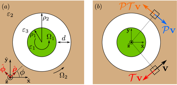
Figure 1: (a) The system under study: a vacuum cavity is delimited by two cylindrical metallic walls that rotate with angular velocities $\Omega_{1}$ and $\Omega_{2}$. (b) Schematic representing the invariance of the system under $\mathcal{PT}$-symmetry. A generic “element” of the rotating body (delimited by the framed box in the bottom region) is transformed under the time reversal operation as $\mathcal{T}\mathbf{v}$, under parity operation as $\mathcal{P}\mathbf{v}$ and under the parity-time operation as $\mathcal{PT}\mathbf{v}$. Here, the parity operator is taken equal to $\mathcal{P}:\left(x,y,z\right)\to\left(x,-y,z\right)$ . From an electromagnetic point of view, the parity-time transformation leads to a structure that has the same response as the original one.

The angular velocities of the cylinders are supposed to be time independent. As discussed in the following, strictly speaking this condition may require the application of an external force to counterbalance a friction-type torque due to possible optical instabilities. In practice, if the metallic walls are sufficiently massive the effect of the friction torque is expected to be negligible in the time scale determined by the growth rate of the electromagnetic fields.

Next, we characterize the cavity’s natural modes with complex oscillation frequencies $\omega=\omega^{\prime}+i\omega^{\prime\prime}$. To do so, we use a purely classical approach to expand the electromagnetic fields in the different cavity regions in cylindrical harmonics and derive the characteristic equation by matching the tangential fields at the interfaces.

It is important to note that different from the case of a body in uniform translational motion silveirinha_theory_2014 ; silveirinha_quantization_2013 ; silveirinha_optical_2014 , a body in uniform circular motion is subject to a centripetal acceleration. Unfortunately there is no simple description of the electromagnetic response of a macroscopic medium in accelerated motion. It is well known that an isotropic uniform (i.e., invariant to translations along the direction of motion) dielectric medium moving with constant velocity ${\bf{v}}=v{\hat{\mathbf{x}}}$ with respect to some inertial frame (the lab frame) is seen as a bianisotropic medium in this reference frame. Indeed, using a relativistic transformation of the fields it is possible to prove that in the lab frame the electromagnetic fields are linked as $\begin{pmatrix}\mathbf{D}\\ \mathbf{B}\end{pmatrix}=\begin{pmatrix}\varepsilon_{0}\overline{\overline{\mathbf{\varepsilon}}}&\frac{1}{c}\overline{\overline{\mathbf{\vartheta}}}\\ \frac{1}{c}\overline{\overline{\mathbf{\zeta}}}&\mu_{0}\overline{\overline{\mathbf{\mu}}}\end{pmatrix}\cdot\begin{pmatrix}\mathbf{E}\\ \mathbf{H}\end{pmatrix}$ with the constitutive parameters given by Kong_book

$$\overline{\overline{\mathbf{\varepsilon}}} =\varepsilon_{t}\left(\overline{\overline{\mathbf{I}}}-\hat{\mathbf{x}}\hat{\mathbf{x}}\right)+\varepsilon~{}\hat{\mathbf{x}}\hat{\mathbf{x}}\rm{,} \varepsilon_{t}=\varepsilon\frac{1-\beta^{2}}{1-n_{m}^{2}\beta^{2}},$$ (1a)

$$\overline{\overline{\mathbf{\mu}}} =\mu_{t}\left(\overline{\overline{\mathbf{I}}}-\hat{\mathbf{x}}\hat{\mathbf{x}}\right)+\mu~{}\hat{\mathbf{x}}\hat{\mathbf{x}}\rm{,} \mu_{t}=\mu\frac{1-\beta^{2}}{1-n_{m}^{2}\beta^{2}},$$ (1b)

$$\overline{\overline{\mathbf{\zeta}}} =-\overline{\overline{\mathbf{\vartheta}}}=-a~{}\hat{\mathbf{x}}\times\overline{\overline{\mathbf{I}}}\rm{,} a=\beta\frac{n_{m}^{2}-1}{1-n_{m}^{2}\beta^{2}},$$ (1c)

being $\beta=v/c$, and $n_{m}^{2}=\varepsilon\mu$, $\varepsilon$ and $\mu$ the material parameters in the rest (comoving) frame. Equations (1a)-(1c) are a direct consequence of formula (76.9) of Ref.landau_electrodynamics_1984 and their detailed derivation can be found in Ref.Kong_book . When the medium is dispersive the parameters $\overline{\overline{\mathbf{\varepsilon}}}$, $\overline{\overline{\mathbf{\mu}}}$, etc, must be evaluated at the Doppler shifted frequency silveirinha_optical_2014 ; silveirinha_spontaneous_2014 . It is relevant to highlight that the material parameters (1a)-(1c) ensure that the plane wave natural modes seen in the lab frame have a dispersion that differs from that seen in the co-moving frame simply by a relativistic Doppler shift transformation. Unfortunately, formulas (1a)-(1c) are difficult to generalize to the case of rotating bodies, mainly because there is no inertial frame wherein a rotating body is instantaneously at rest.

These features greatly complicate the exact physical characterization of the wave phenomena in the cylindrical cavity. Thus, for the sake of simplicity, we will suppose that to a first approximation the transformed constitutive parameters (1a)-(1c) are locally valid at each point of the moving medium. Moreover, we restrict our attention to the quasi-electrostatic limit and to velocities $v=\Omega\rho$ ($\rho$ is the radial distance to the center of the cavity) small with respect to the light velocity $c$, so that the bianisotropic nature of the transformed constitutive parameters can be neglected. Note that in the quasi-static limit the electric field dominates over the magnetic field and this justifies the neglect of the crossed material parameters ($\overline{\overline{\mathbf{\zeta}}},\overline{\overline{\mathbf{\vartheta}}}$). Within these assumptions, equations (1a)-(1c) reduce to $\overline{\overline{\mathbf{\varepsilon}}}\approx\varepsilon$, $\overline{\overline{\mathbf{\mu}}}\approx\mu$, $\overline{\overline{\mathbf{\zeta}}}=-\overline{\overline{\mathbf{\vartheta}}}\approx 0$, and the influence of the rotational motion dwells only in the Doppler shifted frequency $\tilde{\omega_{i}}$:

$$\varepsilon_{i}=\varepsilon_{i}\left({\tilde{\omega}_{i}}\right),\quad\mu_{i}=\mu_{i}\left({\tilde{\omega}_{i}}\right).$$ (2)

Here, $\tilde{\omega_{i}}$ represents the frequency in the frame instantaneously comoving with the relevant point of the $i$-th material with velocity ${\bf{v}}_{i}$. In case of a translational motion along the $x$-direction, it can be related to the frequency $\omega$ in the laboratory frame as $\tilde{\omega_{i}}=\omega-k_{x}v_{i}$ where $k_{x}=-i{\bf{\hat{x}}}\cdot\nabla$ is the wave number along the $x$ direction. For a rotational motion ${\bf{v}}_{i}=\Omega_{i}\rho{\hat{\mathbf{\phi}}}$, and thus it follows that $\tilde{\omega}_{i}=\omega+\Omega_{i}\,i\partial_{\phi}$, where $\partial_{\phi}=\partial/\partial\phi$ is the derivative with respect to the azimuthal angle. The dependence of the constitutive parameters on a spatial derivative ($\partial_{\phi}$) is consistent with the fact that a frequency dispersive medium in motion becomes spatially dispersive. For waves with an azimuthal variation of the form $\text{e}^{in\phi}$ the Doppler shifted frequency is given simply by:

$$\tilde{\omega_{i}}=\omega-n\Omega_{i},$$ (3)

where $n=0,\pm 1,...$ is the azimuthal quantum number. In summary, in the quasi-static limit and under a non-relativistic approximation a dielectric under a rotational motion is characterized in the lab frame by the same material parameters $\varepsilon_{i}$ and $\mu_{i}$ as in the rest frame, but $\varepsilon_{i}$ and $\mu_{i}$ need to be evaluated at the Doppler shifted frequency $\tilde{\omega}_{i}$. In all the examples of the article the materials do not have a magnetic response ($\mu_{i}=1$). We numerically verified (not shown) that this theory applied to the case of metal slabs in relative translational motion gives results consistent with the exact relativistic solution.

Using the proposed formalism it is now a simple task to find the cavity modes. It is clear that because of the cylindrical symmetry the modes can be classified according to the azimuthal variation $\text{e}^{in\phi}$. Here, we are interested in $p$-polarized modes with electric field parallel to the $xoy$ plane and magnetic field directed along the $z$-symmetry axis. An ansatz for the magnetic field in the lab frame is $H_{z}=\text{e}^{in\phi}f_{n}(k\rho)$ with $f_{n}$ a cylindrical Bessel function of the first kind ($J_{n}$) or of the second kind ($Y_{n}$). Hence, taking into account the specific asymptotic conditions to be satisfied in each part of the cavity, the magnetic field in each region of space of Fig. 1 is

$$H_{z}(\rho,\phi)=\text{e}^{in\phi}\left\{\begin{tabular}[]{l l l}$C_{11}J_{|n|}\left(\frac{\omega}{c}\sqrt{\varepsilon_{1}}\rho\right)$,&&$\rho<\rho_{1}$\\ $C_{31}J_{|n|}\left(\frac{\omega}{c}\sqrt{\varepsilon_{3}}\rho\right)+C_{32}Y_{|n|}\left(\frac{\omega}{c}\sqrt{\varepsilon_{3}}\rho\right)$,&&$\rho_{2}>\rho>\rho_{1}$\\ $C_{21}H_{|n|}^{(1)}\left(\frac{\omega}{c}\sqrt{\varepsilon_{2}}\rho\right)$,&&$\rho>\rho_{2}$\end{tabular}\right.$$ (4)

where $H_{n}^{(1)}=J_{n}+iY_{n}$ is the Hankel function of the first kind, and $C_{ij}$ are constant coefficients. The permittivity of each region $\varepsilon_{i}$ is evaluated at the corresponding Doppler shifted frequency $\tilde{\omega}_{i}$. The azimuthal component of the electric field in the $i$-th region is given by

$$E_{\phi}(\rho,\phi) =\frac{1}{i\omega\varepsilon_{0}\varepsilon_{i}\left(\tilde{\omega}_{i}\right)}\cdot\frac{\partial H_{z}}{\partial\rho}(\rho,\phi).$$ (5)

By imposing the continuity of $H_{z}$ and $E_{\phi}$ at the two material-vacuum interfaces, one obtains the following 4 $\times$ 4 homogeneous matricial system (here ^′ represents the derivative with respect to the argument)

$$\begin{pmatrix}J_{|n|}\left(\frac{\omega}{c}\sqrt{\varepsilon_{1}}\rho_{1}\right)&-J_{|n|}\left(\frac{\omega}{c}\sqrt{\varepsilon_{3}}\rho_{1}\right)&-Y_{|n|}\left(\frac{\omega}{c}\sqrt{\varepsilon_{3}}\rho_{1}\right)&0\\ \frac{1}{\sqrt{\varepsilon_{1}}}J^{\prime}_{|n|}\left(\frac{\omega}{c}\sqrt{\varepsilon_{1}}\rho_{1}\right)&-\frac{1}{\sqrt{\varepsilon_{3}}}J^{\prime}_{|n|}\left(\frac{\omega}{c}\sqrt{\varepsilon_{3}}\rho_{1}\right)&-\frac{1}{\sqrt{\varepsilon_{3}}}Y^{\prime}_{|n|}\left(\frac{\omega}{c}\sqrt{\varepsilon_{3}}\rho_{1}\right)&0\\ 0&J_{|n|}\left(\frac{\omega}{c}\sqrt{\varepsilon_{3}}\rho_{2}\right)&Y_{|n|}\left(\frac{\omega}{c}\sqrt{\varepsilon_{3}}\rho_{2}\right)&-H_{|n|}^{(1)}\left(\frac{\omega}{c}\sqrt{\varepsilon_{2}}\rho_{2}\right)\\ 0&\frac{1}{\sqrt{\varepsilon_{3}}}J^{\prime}_{|n|}\left(\frac{\omega}{c}\sqrt{\varepsilon_{3}}\rho_{2}\right)&\frac{1}{\sqrt{\varepsilon_{3}}}Y^{\prime}_{|n|}\left(\frac{\omega}{c}\sqrt{\varepsilon_{3}}\rho_{2}\right)&-\frac{1}{\sqrt{\varepsilon_{2}}}H_{|n|}^{\prime(1)}\left(\frac{\omega}{c}\sqrt{\varepsilon_{2}}\rho_{2}\right)\end{pmatrix}\begin{pmatrix}C_{11}\\ C_{31}\\ C_{32}\\ C_{21}\end{pmatrix}=0$$ (6)

whose nontrivial solutions determine the cavity modes. The natural frequencies of oscillation $\omega=\omega^{\prime}+i\omega^{\prime\prime}$ can be found by setting the determinant of the matrix equal to zero. Because the Bessel functions lead to a transcendental characteristic equation, the calculation of the natural frequencies can only be done with numerical methods. Consistent with the assumptions that led to Eq. (2), we are interested in subwavelength metallic cavities for which $k\rho\ll 1$. As shown next, in this case it is possible to greatly simplify the problem and obtain an approximate algebraic characteristic equation.

Indeed when $k\rho\ll 1$ the asymptotic form of the cylindrical Bessel functions can be used

$$J_{|n|}\left(k\rho\right)\underset{k\rho\ll 1}{\longrightarrow}\alpha_{1}\left(k\rho\right)^{|n|},$$ (7a)

$$Y_{|n|}\left(k\rho\right)\underset{k\rho\ll 1}{\longrightarrow}\alpha_{2}\left(k\rho\right)^{-|n|},$$ (7b)

where $\alpha_{i}$ are constant coefficients and it is assumed that $n\neq 0$. The case $n=0$ is not interesting to us because waves with a zero azimuthal quantum number do not experience a Doppler shift ($\tilde{\omega}_{i}=\omega$ see Eq. (3)), and hence it is evident that for $n=0$ there are no instabilities. In this context, the homogeneous matricial system can be rewritten as

$$\begin{pmatrix}-1&1&1&0\\ -\frac{1}{\varepsilon_{1}}&\frac{1}{\varepsilon_{3}}&-\frac{1}{\varepsilon_{3}}&0\\ 0&\left(\frac{\rho_{2}}{\rho_{1}}\right)^{|n|}&\left(\frac{\rho_{2}}{\rho_{1}}\right)^{-|n|}&-1\\ 0&\frac{1}{\varepsilon_{3}\rho_{1}}\left(\frac{\rho_{2}}{\rho_{1}}\right)^{|n|-1}&\frac{-1}{\varepsilon_{3}\rho_{1}}\left(\frac{\rho_{2}}{\rho_{1}}\right)^{-|n|-1}&\frac{1}{\varepsilon_{2}\rho_{2}}\end{pmatrix}\begin{pmatrix}A_{11}\\ A_{31}\\ A_{32}\\ A_{21}\end{pmatrix}=0,$$ (8)

where $A_{ij}$ are some constant coefficients. The corresponding characteristic equation is:

$$\frac{\left[1-\left(\frac{\rho_{2}}{\rho_{1}}\right)^{2|n|}\right]}{\left[1+\left(\frac{\rho_{2}}{\rho_{1}}\right)^{2|n|}\right]}=\frac{\varepsilon_{1}(\tilde{\omega}_{1})\varepsilon_{3}(\tilde{\omega}_{3})+\varepsilon_{2}(\tilde{\omega}_{2})\varepsilon_{3}(\tilde{\omega}_{3})}{\varepsilon_{1}(\tilde{\omega}_{1})\varepsilon_{2}(\tilde{\omega}_{2})+\varepsilon_{3}^{2}(\tilde{\omega}_{3})}.$$ (9)

Clearly, in this quasi-static approximation [Eq. (9)] the natural oscillation frequencies $\omega=\omega^{\prime}+i\omega^{\prime\prime}$ only depend on the ratio between the radii but not on the specific values of the individual radii. The impact of a finite cavity radius can be investigated by directly solving equation (6). It is important to highlight that Eq. (9) is nothing more than – apart from the Doppler-shifted frequencies in the material parameters – the dispersion of the cavity modes in the quasi-static limit. This observation makes clear that our analysis can be extended in a straightforward manner to other geometries. In the rest of the article, it is assumed that the middle layer is a vacuum ($\varepsilon_{3}=1$), and that the other two materials are modeled by a Drude dispersion model $\varepsilon_{i}(\tilde{\omega}_{i})=1-\omega_{p}^{2}/\left[\tilde{\omega}_{i}(\tilde{\omega}_{i}+i\Gamma)\right]$, being $\omega_{p}$ the plasma frequency and $\Gamma$ the collision frequency.

II.1 Instabilities in the quasi-static limit

In the following, we use the algebraic characteristic equation (9) to characterize the cavity natural frequencies. Figure 2 represents the calculated $\omega$ as a function of the relative angular velocity $\Omega$, for $\Omega_{1}=-\Omega_{2}=\Omega/2$, $n=1$, $\rho_{2}/\rho_{1}=2$ and no material loss ($\Gamma=0$). As seen, for angular velocities greater than a threshold velocity approximately coincident with the plasma frequency of the metal $\omega_{p}$, two of the eigenwaves have complex oscillation frequencies. In particular, one of the modes has $\omega^{\prime\prime}$ with a positive imaginary part corresponding to waves growing with time as $e^{\omega^{\prime\prime}t}$, i.e. to an unstable system.

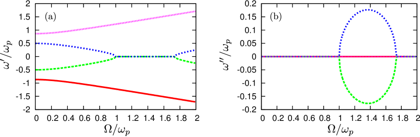
Figure 2: Free oscillation complex frequencies of the cavity $\omega=\omega^{\prime}+i\omega^{\prime\prime}$ for $\Omega_{1}=-\Omega_{2}=\Omega/2$, $n=1$, $\rho_{2}/\rho_{1}=2$ and $\Gamma=0$. (a) $\omega^{\prime}/\omega_{p}$ as a function of $\Omega/\omega_{p}$. (b) $\omega^{\prime\prime}/\omega_{p}$ as a function of $\Omega/\omega_{p}$.

Interestingly, the plot of $\omega^{\prime\prime}$ versus the angular frequency is symmetric with respect to the horizontal axis, such that the complex frequencies occur in pairs $\omega^{\prime}\pm i\omega^{\prime\prime}$. This feature is characteristic of systems with a broken parity-time (${\cal P}{\cal T}$) symmetry bender_pt-symmetric_1999 ; bender_making_2007 ; silveirinha_spontaneous_2014 . Indeed, in case of lossless materials the system of Fig. 1 (a) is invariant under the ${\cal P}{\cal T}$ operation, being the parity operation understood as the transformation $\left({x,y,z}\right)\to\left({x,-y,z}\right)$ (one could as well choose the transformation $\left({x,y,z}\right)\to\left({-x,y,z}\right)$). Note that as illustrated in Fig. 1 (b), the time-reversal operator flips the velocity of the medium silveirinha_spontaneous_2014 , while the parity operator flips the $y$-component of the velocity, and hence the combined ${\cal P}{\cal T}$ operation only flips the $x$-component of the velocity, as it should be so that the medium stays invariant under a coordinate transformation of the form $\left({x,y,z}\right)\to\left({x,-y,z}\right)$. Thus, for a lossless system the emergence of system instabilities is a manifestation of a broken ${\cal P}{\cal T}$-symmetry similar to the planar case studied in Ref. silveirinha_spontaneous_2014 , and implies that the time evolution of electromagnetic waves is described by a non-Hermitian ${\cal P}{\cal T}$-symmetric operator. Unstable natural modes are not invariant under the ${\cal P}{\cal T}$ operation, even though the physical system has that symmetry.

In Fig. 1 the instabilities have a vanishing real part $\omega^{\prime}$ and correspond to a static field, predominantly electric, growing exponentially with time. This feature is specific to the scenario where both cylinders rotate in opposite directions with the same angular velocity.

When the angular velocities of the two materials are asymmetric ($\Omega_{1}+\Omega_{2}\neq 0$) the ratio between the amplitudes of the magnetic and electric fields grows with $\Omega_{1}+\Omega_{2}$, and the frequency $\omega^{\prime}$ is transformed as:

$$\omega^{\prime}\to\omega^{\prime}\left(\Omega\right)+n\frac{{\Omega_{1}+\Omega_{2}}}{2}$$ (10)

where $\Omega\equiv\Omega_{1}-\Omega_{2}$ and $\omega^{\prime\prime}$ remains invariant. The peak value of $\omega^{\prime\prime}$ occurs roughly for $\Omega=1.4\omega_{p}\approx 2\omega_{sp}$, being $\omega_{sp}=\omega_{p}/\sqrt{2}$ the surface plasmon resonance. In particular, when one of the material regions is at rest (let’s say $\Omega_{2}=0$) one gets $\omega^{\prime}\gg\omega^{\prime\prime}$, and the peak instability is associated with $\omega^{\prime}\approx\omega_{sp}$ for the $n=1$ mode. Independent of the value of $\Omega_{1}+\Omega_{2}$, the amplification occurs only in a finite range of frequencies $\omega^{\prime}$ in agreement with the conclusions of refs. zeldovich_generation_1971 ; manjavacas_vacuum_2010 ; maghrebi_spontaneous_2012 ; maghrebi_nonequilibrium_2014 .

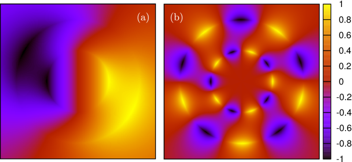
Figure 3: Time snapshot of the real part of the magnetic field $H_{z}$ associated with the instability for $\Omega_{1}=-\Omega_{2}=\Omega/2$ and $\rho_{2}/\rho_{1}=2$. (a) $n=1$ and $\Omega/\omega_{p}=1.37$. (b) $n=5$ and $\Omega/\omega_{p}=0.28$.

A density plot of the magnetic field associated with the strongest instability is depicted in Fig. 3(a). The field has a dipolar symmetry ($n=1$) and the regions of strongest field intensity are concentrated close to the surface of each cylinder, facing each other. This observation together with the fact that the instabilities are developed for $\Omega\approx 2\omega_{sp}$ demonstrates that the field exponential growth with time is due to the interaction of surface plasmon polaritons in each cylinder, similar to what happens in the planar case silveirinha_quantization_2013 ; silveirinha_optical_2014 ; silveirinha_theory_2014 ; silveirinha_spontaneous_2014 . The field exponential growth can be pictured as being due to the interaction of positive frequency harmonic oscillators and negative frequency harmonic oscillators, such that $\tilde{\omega}_{1}$ and $\tilde{\omega}_{2}$ have opposite signs silveirinha_quantization_2013 ; silveirinha_optical_2014 . This interaction is made possible by the relative rotation of the two cylinders. Oscillators associated with negative frequencies behave as energy reservoirs that may serve to pump the oscillations of the system and generate the unstable behavior frolov_excitation_1986 ; silveirinha_quantization_2013 ; silveirinha_optical_2014 ; Horshley2 ; Jacob . For example, when $\Omega_{2}=0$ it can be checked that $\tilde{\omega}_{1}<0$ and $\tilde{\omega}_{2}>0$ in the entire instability region, and thus the moving region may be regarded as the energy reservoir. In addition, the plasmonic nature of the interaction can be seen by noting that the peak instability occurs for $\tilde{\omega}_{1}\approx-\omega_{sp}$ and $\tilde{\omega}_{2}\approx\omega_{sp}$. It is instructive to note that for a translational motion an unstable behavior requires the coupling of two oscillators (interaction of two different bodies in relative motion) because with a single moving body it is always possible to switch to a frame where the body is at rest, and where evidently instabilities are impossible to occur silveirinha_quantization_2013 . In principle, for a rotational motion the instabilities may occur even with a single body because a rotating body is in motion in any inertial frame. However, if the velocity of rotation is sufficiently small, as implicit in our theory, the interaction between different parts of the same body is ineffective, and similar to the case of a translational motion two interacting bodies (two different oscillators) are required to trigger the instability. Indeed, for a single rotating cylinder surrounded by a vacuum (the limit $\rho_{2}\to\infty$ and $\varepsilon_{3}=1$) Eq. (9) reduces to $\varepsilon_{1}(\tilde{\omega}_{1})+1=0$, which evidently does not lead to any instability.

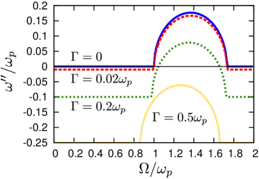
Figure 4: Influence of the metal damping (collision) frequency $\Gamma$ on $\omega^{\prime\prime}$ for the mode associated with the unstable behavior for $\Omega_{1}=-\Omega_{2}=\Omega/2$, $n=1$ and $\rho_{2}/\rho_{1}=2$.

It is interesting to see how the material loss affects the natural oscillation frequencies, and in particular whether the instabilities withstand realistic plasmonic loss. This study is reported in Fig. 4 which depicts the imaginary part of the free oscillation frequency (for the mode with positive $\omega^{\prime\prime}$) as a function of the normalized angular velocity. The effect of damping is roughly equivalent to adding a negative constant imaginary part to the value of $\omega^{\prime\prime}$ that reduces the strength of the growth rate. It is relevant to mention that in the presence of material loss the system is not anymore ${\cal P}{\cal T}$-symmetric, and hence the frequency spectrum does not have the complex conjugation symmetry as in Fig. 2. The range of angular velocities $\Omega$ for which $\omega^{\prime\prime}>0$ becomes narrower with increasing $\Gamma$, up to a point wherein all the oscillations are damped ($\omega^{\prime\prime}<0$) and the instability ceases. Importantly, the unstable behavior is quite robust to the effect of material loss and is observed even for collision frequencies much larger than those characteristic of realistic metals ($0.01<\Gamma/\omega_{p}<0.2$). Furthermore, since the instabilities result from the hybridization of evanescent waves attached to the individual cylinders, they are strongly dependent on the value of $\rho_{2}/\rho_{1}$ and the material loss may be partially compensated by narrowing the vacuum gap.

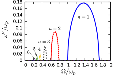
Figure 5: Evolution of $\omega^{\prime\prime}$ with the azimuthal quantum number $n$ for the mode associated with the unstable behavior and $\Omega_{1}=-\Omega_{2}=\Omega/2$, $\rho_{2}/\rho_{1}=2$ and $\Gamma=0$.

The influence of the quantum azimuthal number $n$ on the strength of the instabilities is investigated in Fig. 5 for the case $\Omega_{1}=-\Omega_{2}=\Omega/2$. It is seen that the strength of the instabilities progressively decreases with $n$ and is negligible for high $n$. This can be understood noting that modes with a large $n$ result from the hybridization of tightly confined surface plasmons that overlap weakly in the vacuum gap as illustrated in Fig. 3(b) for $n=5$. Stronger instabilities are obtained for a smaller gap. Remarkably, the threshold angular velocity for the unstable behavior scales roughly as $1/n$ and hence decreases with the azimuthal quantum number. In particular, the angular velocity for which the unstable behavior is stronger is $\Omega\approx 2\omega_{sp}/n$. In case one of the bodies is at rest (e.g., $\Omega_{2}=0$) the peak instability is always associated with the frequency $\omega^{\prime}\approx\omega_{sp}$, independent of the value of $n$.

Due to the reality of the electromagnetic field, the spectrum associated with negative values of $n$ is linked to the spectrum associated with positive values of $n$ as $\omega\to-\omega^{*}$, such that the real part of the frequency is flipped, while the imaginary part is unchanged. In the case wherein $\Omega_{2}=0$, the unstable modes with $\omega^{\prime}>0$ occur for azimuthal quantum numbers $n$ with the same sign as $\Omega_{1}$. An intuitive explanation is that the spontaneous light emission by a rotating body favors physical channels associated with angular variations in the direction determined by the moving body.

II.2 Effect of time retardation

It is important to have some idea of the impact of time retardation effects. Figure 6 shows a comparison between the quasi-static theory and the results obtained by setting the determinant of the matrix in Eq. (6) equal to zero. In this plot, the structural parameters are as in the previous section, namely $\rho_{2}/\rho_{1}=2$, and only the mode $n=1$ with positive imaginary part is represented. As seen, as soon as the radii of the cylinders become of the order of $c/\omega_{p}$, the quasi-static approximation breaks down and the time retardation effects play some role. The effect of time retardation is to reduce the strength of the instabilities. The threshold for the emergence of instabilities is unaffected by the time retardation.

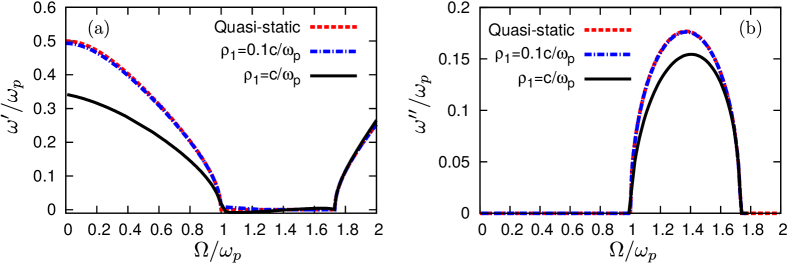
Figure 6: Comparison between the “exact” ($\rho_{1}=c/\omega_{p}$ and $\rho_{1}=0.1c/\omega_{p}$) and the quasi-static free oscillation complex frequencies of the cavity $\omega=\omega^{\prime}+i\omega^{\prime\prime}$ for the mode with positive imaginary part. Here $n=1$, $\rho_{2}/\rho_{1}=2$ and $\Gamma=0$. (a) $\omega^{\prime}/\omega_{p}$ as a function of $\Omega/\omega_{p}$. (b) $\omega^{\prime\prime}/\omega_{p}$ as a function of $\Omega/\omega_{p}$.

II.3 Wave energy

From the Poynting theorem in the time domain, it is simple to show that for a closed cavity and in the absence of external current sources the quantity $E_{w}=\int^{t}dt\int\limits_{\text{all space}}dV\left(\mathbf{E}\cdot\frac{\partial\mathbf{D}}{\partial t}+\mathbf{H}\cdot\frac{\partial\mathbf{B}}{\partial t}\right)$ must be time independent. It is implicitly assumed that the angular velocity of the rotating bodies is time-invariant. For lossless materials $E_{w}$ can be identified with the total wave energy of the system, which includes the electromagnetic energy and part of the energy associated with the kinetic degrees of freedom of the system (see Ref.silveirinha_theory_2014 for a detailed discussion). For time-harmonic fields $\mathbf{E}=\text{Re}\left\{\mathbf{E}_{\omega}\text{e}^{-i\omega t}\right\}$, $\mathbf{D}=\text{Re}\left\{\mathbf{D}_{\omega}\text{e}^{-i\omega t}\right\}$, etc, it is straightforward to check that $E_{w}=E_{w0}(t)\text{e}^{2\omega^{\prime\prime}t}$ where $E_{w0}(t)$ is a periodic function of time with period $\pi/\omega^{\prime}$. The time averaged value of $E_{w0}(t)$ is given by $E_{w0,\text{av}}=\int\limits_{\text{all space}}W_{\text{av}}~{}dV$ where

$$W_{\text{av}}=\frac{1}{4}\text{Re}\left\{\mathbf{D}_{\omega}\cdot\mathbf{E}_{\omega}^{\ast}\frac{\omega}{i\omega^{\prime\prime}}\right\}+\frac{1}{4}\text{Re}\left\{\mathbf{B}_{\omega}\cdot\mathbf{H}_{\omega}^{\ast}\frac{\omega}{i\omega^{\prime\prime}}\right\}$$ (11)

is the time-averaged wave energy density envelope. For a weak instability $\omega^{\prime\prime}\ll\omega^{\prime}$ (limit $\omega^{\prime\prime}\to 0$) and within the approximations implicit in Eq. (2) the wave energy density reduces to $W_{\text{av}}=\frac{1}{4}\mathbf{E}_{\omega}\cdot\mathbf{E}_{\omega}^{\ast}\frac{\partial}{\partial\omega}\left[\varepsilon\omega\right]+\frac{1}{4}\mathbf{H}_{\omega}\cdot\mathbf{H}_{\omega}^{\ast}\frac{\partial}{\partial\omega}\left[\mu\omega\right]$, consistent with a well-known electromagnetic theory result landau_electrodynamics_1984 . In the quasi-static limit the field is predominantly electric and hence:

$$W_{\text{av}} \approx\frac{1}{4}\mathbf{E}_{\omega}\cdot\mathbf{E}_{\omega}^{\ast}\frac{\partial}{\partial\omega}\left[\varepsilon\omega\right]_{\omega=\omega^{\prime}}$$

$$=\frac{1}{4}\mathbf{E}_{\omega}\cdot\mathbf{E}_{\omega}^{\ast}\frac{\partial}{\partial\omega}\left[\varepsilon(\mathbf{r},\omega-n\Omega)\omega\right]_{\omega=\omega^{\prime}}.$$ (12)

In Figure 7 we plot $\frac{\partial}{\partial\omega}\left[\varepsilon(\omega-n\Omega)\omega\right]_{\omega=\omega^{\prime}}$ for a Drude plasma as a function of frequency for different values of the angular velocity and assuming a dipolar mode ($n=1$).

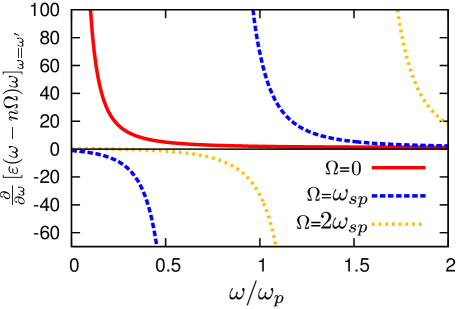
Figure 7: Plot of $\frac{\partial}{\partial\omega}\left[\varepsilon(\omega-n\Omega)\omega\right]_{\omega=\omega^{\prime}}$ as a function of the normalized frequency for $\Omega=0$, $\omega_{sp}$ and $2\omega_{sp}$ and a dipolar interaction ($n$=1). The function is negative for $0<\omega<\Omega$ .

As seen, for nonzero angular velocities $\frac{\partial}{\partial\omega}\left[\varepsilon(\omega-n\Omega)\omega\right]_{\omega=\omega^{\prime}}$ can become negative, i.e., the wave energy density can be negative in a moving region. In that case, an increase of the electric field intensity leads to a decrease of the local wave energy. These findings are completely consistent with the results of Refs.silveirinha_quantization_2013 ; silveirinha_theory_2014 ; Horshley , where it was shown that the wave energy density has no lower bound in a material that moves with a velocity that exceeds the Cherenkov limit. This theory provides an intuitive explanation of the reason why the instabilities are associated with two oscillators with oppositely signed frequencies. Indeed, in case of an unstable behavior (growing exponential) the total wave energy of the system can be time-independent only if $E_{w0,\text{av}}=0$ . Thus, an oscillator with positive frequency is required to increase its wave energy in the exact same proportion as the oscillator with negative frequency decreases the energy, so that the total wave energy remains time independent. Note that even though the total wave energy is time independent, the wave energy density varies with time and in space due to the energy transfer between the two bodies under rotation.

III Torque

An obvious question is: what is the mechanism that pumps the unstable modes? Is it rooted, similarly to the planar case silveirinha_theory_2014 , in the conversion of kinetic energy into electromagnetic energy? Next, it is confirmed that this is indeed the case, and to demonstrate such a property we determine the mechanical torque induced by the instabilities.

The instantaneous force per unit of volume induced by the electromagnetic field is stratton_electromagnetic_2007

$$\mathbf{f}=\nabla\cdot\overline{\overline{\mathbf{T}}}-\frac{\partial}{\partial t}\mathbf{g_{\rm{EM}}},$$ (13)

where $\mathbf{g_{\rm{EM}}}$ is the electromagnetic momentum density and $\overline{\overline{\mathbf{T}}}$ the Maxwell stress tensor. The torque $\boldsymbol{\tau}$ resulting from the force $\mathbf{f}$ is then given by

$$\boldsymbol{\tau}=\int\mathbf{r}\times\mathbf{f}~{}d^{3}\mathbf{r}=\int\mathbf{r}\times\left(\nabla\cdot\overline{\overline{\mathbf{T}}}-\frac{\partial}{\partial t}\mathbf{g_{\rm{EM}}}\right)~{}d^{3}\mathbf{r}.$$ (14)

where $\mathbf{r}$ is the position vector. Integrating by parts, it is possible to write the contribution of the stress-tensor as an integral over the surface of the relevant body (at the air side):

$$\boldsymbol{\tau}=\int{{\bf{r}}\times\left({{\boldsymbol{\hat{\nu}}}\cdot\overline{\overline{\bf{T}}}}\right)\,}ds-\int\mathbf{r}\times\frac{\partial}{\partial t}\mathbf{g_{\rm{EM}}}~{}d^{3}\mathbf{r}.$$ (15)

Here, $\boldsymbol{\hat{\nu}}$ is a unit vector oriented towards the outside of the body, and we use the fact that $\sum\limits_{i}{{\bf{\hat{u}}}_{i}\cdot\overline{\overline{\bf{T}}}\times{\bf{\hat{u}}}_{i}}=0$, being ${\bf{\hat{u}}}_{i}$ a generic unit vector along the Cartesian coordinate axes, because the stress tensor is symmetric. Because in the surface integral the stress-tensor is evaluated at the air side of the interface we can use the standard formula

$$\overline{\overline{\mathbf{T}}}=\varepsilon_{0}\mathbf{E}\otimes\mathbf{E}+\mu_{0}\mathbf{H}\otimes\mathbf{H}-1/2\left(\varepsilon_{0}|\mathbf{E}|^{2}+\mu_{0}|\mathbf{H}|^{2}\right)\overline{\overline{\mathbf{I}}}.$$ (16)

Clearly, in time harmonic regime the torque (which is a quadratic function of the electromagnetic fields) grows exponentially as $e^{2\omega^{\prime\prime}t}$. Hence, we can write $\boldsymbol{\tau}=\boldsymbol{\tau}_{0}\left(t\right)e^{2\omega^{\prime\prime}t}$, being $\boldsymbol{\tau}_{0}$ the envelope of the torque which typically has a component that oscillates in time with frequency $2\omega^{\prime}$. The definition of the electromagnetic momentum density in material media is surrounded by a century-old controversy pfeifer_textbf_2007 ; barnett_resolution_2010 . We can avoid this controversy by calculating time-averaged torque, obtained by time-averaging the envelope of the torque: $\left\langle{\boldsymbol{\tau}}\right\rangle={\boldsymbol{\tau}}_{0,{\rm{av}}}e^{2\omega^{\prime\prime}t}$. It is simple to check that with this definition one has $\left\langle\frac{\partial\mathbf{g_{\rm{EM}}}}{\partial t}\right\rangle=0$, and hence it is finally found that:

$${\boldsymbol{\tau}}_{0,{\rm{av}}}=\frac{1}{2}{\mathop{\rm Re}\nolimits}\left\{{\int{{\bf{r}}\times\left({{\boldsymbol{\hat{\nu}}}\cdot\overline{\overline{\bf{T}}}_{c}}\right)\,}ds}\right\}$$ (17)

where $\overline{\overline{\mathbf{T}}}_{c}=\varepsilon_{0}\mathbf{E}_{\omega}\otimes\mathbf{E}_{\omega}^{*}+\mu_{0}\mathbf{H}_{\omega}\otimes\mathbf{H}_{\omega}^{*}-1/2\left(\varepsilon_{0}|\mathbf{E}_{\omega}|^{2}+\mu_{0}|\mathbf{H}_{\omega}|^{2}\right)\overline{\overline{\mathbf{I}}}$ is a complex stress tensor written in terms of the complex vector field amplitudes.

Let us apply this theory to the scenario considered in section II wherein the material 2 is at rest ($\Omega_{2}=0$) and the material 1 rotates with angular velocity $\Omega_{1}=\Omega$. Straightforward calculations show that the time-averaged torque per unit of length is

$$\frac{\left\langle\boldsymbol{\tau}\right\rangle}{h} =2\pi\rho_{1}^{2}\frac{\varepsilon_{0}}{2}{\mathop{\rm Re}\nolimits}\left\{{E_{\omega,\rho}(\rho_{1})E_{\omega,\theta}^{*}(\rho_{1})}\right\}e^{2\omega^{\prime\prime}t}~{}\hat{\mathbf{z}},$$ (18)

where $h$ is the height of the cylinder. This formula shows that the torque can be roughly estimated as $\left\langle\boldsymbol{\tau}\right\rangle\sim{\boldsymbol{\varepsilon}}_{E}\text{e}^{2\omega^{\prime\prime}t}$ where ${\boldsymbol{\varepsilon}}_{E}$ is the electric energy stored in the air cavity at time $t=0$. Hence, in the time scale determined by $1/\omega^{\prime\prime}$ the mechanical torque is typically small, and becomes relevant only when $t\gg 1/\omega^{\prime\prime}$ due to the exponential growth.

The time-averaged torque calculated with the quasi-static approximation for the mode with positive imaginary part (the unstable mode) is represented in Fig. 8 as a function of the angular velocity at a given instant of time.

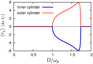
Figure 8: Normalized time averaged torque (in arbitrary units) acting on the inner and outer cylinders as a function of the angular velocity for $\rho_{2}/\rho_{1}=2$, $\Omega_{1}=\Omega$, $\Omega_{2}=0$ and lossless plasmonic materials $\Gamma=0$.

In the numerical simulation it is assumed that only the inner cylinder is rotating and that $n=1$, $\rho_{2}/\rho_{1}=2$ and $\Gamma=0$. As seen in section II, in this situation the instabilities are developed for angular velocities larger than $\omega_{p}$ due to the interaction of the SPPs supported by each surface and associated with $\tilde{\omega}_{1}<0$ and $\tilde{\omega}_{2}>0$. By comparing Figs. 2 and 8, it is seen that the torque is intimately linked to these instabilities since it is non zero only for the angular velocities for which the system is unstable. Importantly, the torque acting on the inner-cylinder is negative and therefore acts against the rotational motion: it is a friction-type torque. The torque acting on the outer-cylinder is exactly the opposite and tends to drag the outer-cylinder into motion, thereby reducing the relative angular velocity between the cylinders. This result confirms that the emergence of instabilities in the system has its origin in the conversion of kinetic energy into electromagnetic energy. Hence, as mentioned in the introduction, to keep the angular velocity constant a positive torque needs to be applied to the inner cylinder in order to counterbalance this friction-type torque. The results of this section further highlight the intimate connection between electromagnetic friction and the coupling between oscillators with positive and negative frequencies in agreement with previous studies Horshley ; silveirinha_quantization_2013 ; silveirinha_optical_2014 ; silveirinha_theory_2014 .

IV Unidirectional light flow

A moving medium is not invariant under a time-reversal transformation, and consequently it is characterized by a nonreciprocal electromagnetic response. This property raises interesting possibilities in the context of asymmetric light flows, which are otherwise generally forbidden in conventional reciprocal media (e.g., isotropic dielectrics and metals at rest) jalas_what_2013 .

An intuitive picture of the effect of motion is that the phase velocity depends if the wave propagates downstream or upstream with respect to the flow of matter Stas_Cherenkov ; philbin_fiber-optical_2008 . As discussed next, this feature can be explored to design a light “circulator”. A circulator is a nonreciprocal three-port network, that is ubiquitous in microwave technology pozar_microwave_2011 . Circulators are also useful at optical frequencies for optical switching and for the optical isolation of the light source from the optical channel. potton_reciprocity_2004 ; jalas_what_2013 . A circulator ideally only allows transmission from port 1 to 3 or from port 3 to 2 or from port 2 to 1 (see Fig. 9; in the figure it is implicit that optical waveguides are connected to the cylindrical cavity at the relevant ports). The propagation in the opposite azimuthal direction (e.g., from port 1 to port 2) is forbidden.

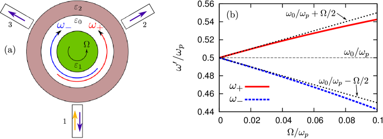
Figure 9: (a) Schematic of the optical circulator with the incoming signal represented by the orange (light gray) arrow and the outgoing waves by the purple (dark gray) arrows. (b) Modes of the cylindrical cavity as a function of the normalized angular velocity for $\rho_{2}/\rho_{1}=2$, $\Omega_{1}=\Omega$, $\Omega_{2}=0$ and $\Gamma=0.01\cdot\omega_{p}$.

In conventional circulators, the unidirectional light flow relies on the existence of constructive or destructive interference patterns at each output, arising from the different oscillation frequency of the modes circulating in the clockwise or anti-clockwise directions in the cavity. Usually the mode splitting is achieved due to a Zeeman-type effect when magnetic materials (e.g., ferrites and some garnets pozar_microwave_2011 ) are biased by a static magnetic field. Because of the drawbacks in terms of size and weight of permanent magnets, different approaches free of magnetic elements have been recently proposed kodera_artificial_2011 ; sounas_electromagnetic_2013 ; sounas_giant_2013 ; sounas_angular-momentum-biased_2014 ; estep_magnetic-free_2014 ; estep_magnetless_2016 .

In what follows, we theoretically demonstrate a new paradigm for an optical circulator based on a cavity with rotating walls. A related result was recently reported for the acoustic case fleury_sound_2014 . Remarkably, this effect is neither based on wave instabilities in the cavity nor on the excitation of SPPs in each slab, but rather on the modal asymmetry between the waves propagating in the direction of rotation ($n=+1$) and in the counter propagating direction ($n=-1$) wang_magneto-optical_2005 ; fleury_sound_2014 ; sounas_giant_2013 ; sounas_angular-momentum-biased_2014 ; estep_magnetic-free_2014 ; fleury_subwavelength_2015 ; estep_magnetless_2016 . Indeed, it can be shown using equation (9) that at small velocities ($\Omega\ll\omega_{p}$) one of the resonant frequencies of the cavity is approximately given by

$$\omega_{n}\approx\omega_{0}+\frac{n\Omega}{2}-i\frac{\Gamma}{2},$$ (19)

where $\omega_{0}=\omega_{sp}\sqrt{1-\left(\frac{\rho_{1}}{\rho_{2}}\right)^{\left|n\right|}-\frac{\Gamma^{2}}{2\omega_{p}^{2}}}$ is the resonant frequency of the cavity when the walls are at rest. Then it follows that the natural frequency of oscillation for the modes associated with $n=\pm 1$ linearly split as

$$\omega_{\pm}\approx\omega_{0}\pm\frac{\Omega}{2}.$$ (20)

This behavior is illustrated in Fig. 9 where the evolution of the natural frequencies with the normalized angular velocity is represented for a resonator with $\rho_{2}/\rho_{1}=2$, $\Omega_{1}=\Omega$, $\Omega_{2}=0$ and $\Gamma=0.01\cdot\omega_{p}$. As seen, the motion of the inner cylinder induces a splitting of the modes, linear in $\Omega$ at small angular velocities, and somewhat analogous to the Zeeman splitting obtained with magnetic materials. The splitting can be understood noting that the resonance condition is roughly of the form $\omega l/v_{p}=2\pi$, where $l\approx\pi(\rho_{1}+\rho_{2})$ is the mean perimeter of the cavity and $v_{p}$ is the SPP phase velocity in the cavity, which depends on the azimuthal quantum number. Because of the Fresnel drag one may expect that when $\Omega>0$ the velocity $v_{p}$ is larger for modes associated with positive $n$ as compared to a mode with index $-n$. Thus, this indicates that $\omega_{+}>\omega_{-}$, consistent with the analytical model.

When the circulator is excited in port 1, the transmissivities for ports 2 and 3 depend on the frequencies of the cavity modes as follows (the formula below corrects a typo in Ref. fleury_sound_2014 ) wang_magneto-optical_2005 ; fleury_sound_2014

$$T_{1\to 2} =\left|\frac{2}{3}\left(\frac{\text{e}^{-i\frac{2\pi}{3}}}{1-i(\omega-\omega_{-})/\gamma_{-}}+\frac{\text{e}^{-i\frac{4\pi}{3}}}{1-i(\omega-\omega_{+})/\gamma_{+}}\right)\right|^{2}$$ (21a)

$$T_{1\to 3} =\left|\frac{2}{3}\left(\frac{\text{e}^{-i\frac{4\pi}{3}}}{1-i(\omega-\omega_{-})/\gamma_{-}}+\frac{\text{e}^{-i\frac{2\pi}{3}}}{1-i(\omega-\omega_{+})/\gamma_{+}}\right)\right|^{2}$$ (21b)

where $\omega_{\pm}$ and $-\gamma_{\pm}$ are the real and imaginary parts of the natural mode frequencies $\omega_{n}$ associated with $n=\pm 1$. Using the approximate expression (19) for $\omega_{n}$, we find that for $\omega=\omega_{0}$ and $\Omega=\Gamma/\sqrt{3}$ one has $T_{1\to 2}=0$ and $T_{1\to 3}=1$ and thus the system behaves as an ideal circulator. Remarkably, the energy flow in the circulator is towards the direction opposite to that of the motion the inner cylinder.

To confirm this result, a density plot of the transmissivities is shown in Fig. 10 as a function of the normalized frequency and of the normalized angular velocity, for the same structural parameters as in Fig. 9.

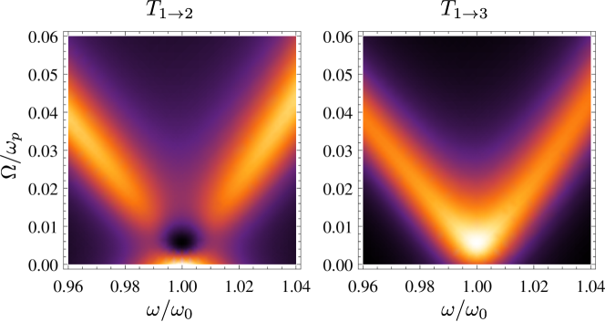
Figure 10: Density plot of the transmissivities $T_{1\to 2}$ and $T_{1\to 3}$ as a function of the normalized frequency $\omega$ and of the normalized angular velocity $\Omega$. Here, $\omega_{0}$ is the resonance frequency when the walls are at rest. The cavity has the same structural parameters as in Fig. 9. Brighter (darker) colours represent a stronger (weaker) transmission.

As seen in the figure, there is a region near to $\omega\approx\omega_{0}$ and $\Omega\approx\Gamma/\sqrt{3}$ where simultaneously $T_{1\to 2}$ goes to zero and $T_{1\to 3}$ goes to 1. In this regime, the moving cavity is strongly non-reciprocal and behaves as an ideal circulator. The corresponding transmission curves for an angular velocity close to the optimal angular velocity $\Omega=\Gamma/\sqrt{3}$ are represented in Fig. 11 as a function of frequency.

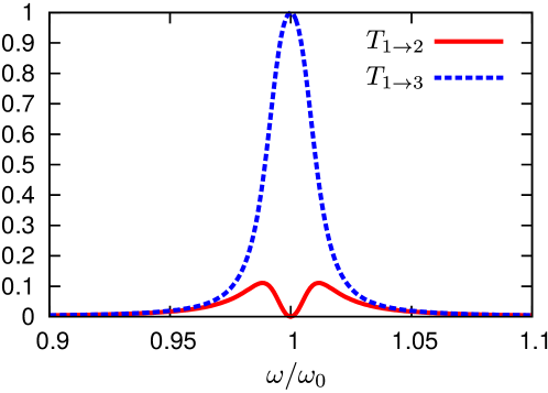
Figure 11: Transmissivities $T_{1\to 2}$ and $T_{1\to 3}$ as a function of the normalized frequency for the optimal angular velocity $\Omega=\Gamma/\sqrt{3}$ and a plasma collision frequency $\Gamma=0.01\cdot\omega_{p}$. The structural parameters of the cavity are the same as in Figs. 9 and 10.

Interestingly, the optimal angular velocity depends only on the level of loss in the plasmonic material, and is smaller for resonances with high quality factor. In an optical design relying on plasmonic materials, in the best scenario it can be about three orders of magnitude smaller than the plasma frequency. Thus, typically the angular velocity required for the cavity to operate as an optical circulator lies well below the threshold associated with electromagnetic instabilities. This puts into evidence that the regime wherein the wave has strongly asymmetric azimuthal flows is independent of the regime wherein the instabilities are developed.

V Discussion and Conclusion

It is important to discuss the practical feasibility of the light generator/amplifier or optical circulator studied in the previous sections. Remarkably, the angular velocities required to obtain optical instabilities are comparable to the metal plasma frequency, and in the best case scenario are about three orders of magnitude smaller for an optical circulator. To our best knowledge, the highest angular velocities ever reached experimentally are reported in arita_laser-induced_2013 , where a circularly polarized laser impinging on a birefringent particle produces an angular velocity of the order of the $\mathrm{M}\mathrm{Hz}$. This value is far from reaching the plasma frequencies of metals that typically are in the UV range west_searching_2010 , or the plasma frequency of semiconductors such as InSb that are in the T Hz   range palik_handbook_1991 ; zhao_rotational_2012 . Consequently, a direct laboratory verification of the concepts proposed in this paper appears unfeasible with the available technology.

Yet, there may be a way to overcome these difficulties. Indeed, we envision that the physical motion of neutral bodies can be mimicked by an electron drift (electrons flowing on a positive ion background) induced by a DC generator. A preliminary assessment of this idea was reported in Ref. morgado_spontaneous_2015 , where it was demonstrated that the physics of the two systems is rather similar in the planar case. The emergence of electromagnetic instabilities due to an electron drift was also discussed in Refs. riyopoulos_thz_2005 ; sydoruk_terahertz_2010 , where instabilities were found at T Hz   frequencies due to the interaction of drifting electrons with lattice waves within the same high mobility semiconductor. The analogies between the two platforms may offer a viable alternative to the actual motion of neutral matter and may allow for the experimental verification of the effects discussed in this article. These ideas will be investigated in future work.

In summary, we studied the conditions under which a pair of plasmonic cylinders rotating past one another develop wave instabilities due to the hybridization of the surface plasmon polaritons supported by the individual cylinders. The characteristic equation for the system natural modes was found, and it was shown that for certain cylindrical harmonics, when the angular velocity surpasses a threshold value comparable to the plasma frequency, some natural modes may have a positive imaginary part corresponding to a wave amplitude growing with time. The instabilities were shown to be robust with respect to realistic material losses. By computing the mechanical torque acting on the cylinders, it was demonstrated that analogous to the planar case, the wave amplification corresponds to a conversion of kinetic energy into electromagnetic radiation and is observed as long as the velocity of rotation is kept above the threshold.

We also investigated the possibility of having a strongly asymmetric light transmission relying on the rotation of the cavity walls. It was shown that the motion of the walls induces a frequency split of the cavity modes that results in a strong nonreciprocal behavior that can serve to design an optical circulator. The optimal angular frequency of rotation is determined by the quality factor of the cavity. Cavities with larger quality factors require lower angular velocities, and hence are the most interesting platform to demonstrate our designs. Finally, we suggested that the behavior of the moving walls may be mimicked by an electron drift induced by a DC voltage generator. This concept can provide a practical roadmap to verify and explore the proposed ideas at terahertz frequencies.

- (1) V. V. Dodonov, “Current status of the dynamical Casimir effect,” Physica Scripta, vol. 82, no. 3, p. 038105, 2010.
- (2) S. A. Fulling and P. C. W. Davies, “Radiation from a Moving Mirror in Two Dimensional Space-Time: Conformal Anomaly,” Proceedings of the Royal Society of London A: Mathematical, Physical and Engineering Sciences, vol. 348, pp. 393–414, 1976.
- (3) V. P. Frolov and V. L. Ginzburg, “Excitation and radiation of an accelerated detector and anomalous doppler effect,” Physics Letters A, vol. 116, pp. 423–426, 1986.
- (4) J. Schwinger, “Casimir energy for dielectrics,” Proceedings of the National Academy of Sciences, vol. 89, pp. 4091–4093, 1992.
- (5) G. Barton and C. Eberlein, “On Quantum Radiation from a Moving Body with Finite Refractive Index,” Annals of Physics, vol. 227, pp. 222–274, 1993.
- (6) G. Barton, “The Quantum Radiation from Mirrors Moving Sideways,” Annals of Physics, vol. 245, pp. 361–388, 1996.
- (7) C. Eberlein, “Sonoluminescence as Quantum Vacuum Radiation,” Physical Review Letters, vol. 76, pp. 3842–3845, 1996.
- (8) S. I. Maslovski, “Casimir repulsion in moving media,” Physical Review A, vol. 84, p. 022506, Aug. 2011.
- (9) M. F. Maghrebi, R. Golestanian, and M. Kardar, “Scattering approach to the dynamical Casimir effect,” Physical Review D, vol. 87, p. 025016, 2013.
- (10) E. V. Teodorovich, “On the Contribution of Macroscopic Van Der Waals Interactions to Frictional Force,” Proceedings of the Royal Society of London A: Mathematical, Physical and Engineering Sciences, vol. 362, pp. 71–77, 1978.
- (11) L. S. Levitov, “Van Der Waals’ Friction,” EPL (Europhysics Letters), vol. 8, no. 6, p. 499, 1989.
- (12) V. E. Mkrtchian, “Interaction between moving macroscopic bodies: viscosity of the electromagnetic vacuum,” Physics Letters A, vol. 207, pp. 299–302, 1995.
- (13) J. B. Pendry, “Shearing the vacuum - quantum friction,” Journal of Physics: Condensed Matter, vol. 9, p. 10301, 1997.
- (14) A. I. Volokitin and B. N. J. Persson, “Theory of friction: the contribution from a fluctuating electromagnetic field,” Journal of Physics: Condensed Matter, vol. 11, no. 2, p. 345, 1999.
- (15) A. I. Volokitin and B. N. J. Persson, “Near-field radiative heat transfer and noncontact friction,” Reviews of Modern Physics, vol. 79, pp. 1291–1329, 2007.
- (16) K. A. Milton, J. S. Høye, and I. Brevik, “The Reality of Casimir Friction,” Symmetry, vol. 8, p. 29, 2016.
- (17) S. A. R. Horsley, “Canonical quantization of the electromagnetic field interacting with a moving dielectric medium,” Phys. Rev. A, vol. 86, p. 023830, 2012.
- (18) J. S. Høye and I. Brevik, “Casimir friction at zero and finite temperatures,” Eur. Phys. J. D, vol. 61, p. 61, 2014.
- (19) J. S. Høye and I. Brevik, “Casimir friction between dense polarizable media,” Entropy, vol. 15, p. 3045, 2013.
- (20) J. S. Høye and I. Brevik, “Casimir friction: Relative motion more generally,” J. Phys.: Condensed Matter, vol. 27, p. 214008, 2015.
- (21) T. G. Philbin and U. Leonhardt, “No quantum friction between uniformly moving plates,” New Journal of Physics, vol. 11, p. 033035, 2009.
- (22) J. B. Pendry, “Quantum friction - fact or fiction?,” New Journal of Physics, vol. 12, p. 033028, 2010.
- (23) U. Leonhardt, “Comment on ’Quantum Friction-Fact or Fiction?’,” New Journal of Physics, vol. 12, no. 6, p. 068001, 2010.
- (24) J. B. Pendry, “Reply to comment on ’Quantum friction-fact or fiction?’,” New Journal of Physics, vol. 12, no. 6, p. 068002, 2010.
- (25) M. G. Silveirinha, “Theory of quantum friction,” New Journal of Physics, vol. 16, p. 063011, 2014.
- (26) M. G. Silveirinha, “Quantization of the electromagnetic field in nondispersive polarizable moving media above the Cherenkov threshold,” Physical Review A, vol. 88, p. 043846, 2013.
- (27) G. Pieplow and C. Henkel, “Cherenkov friction on a neutral particle moving parallel to a dielectric,” J. Phys. Condens. Matter., vol. 27, p. 214001, 2015.
- (28) M. F. Maghrebi, R. Golestanian, and M. Kardar, “Quantum cherenkov radiation and noncontact friction,” Phys. Rev. A, vol. 88, p. 042509, 2013.
- (29) M. G. Silveirinha, “Optical Instabilities and Spontaneous Light Emission by Polarizable Moving Matter,” Physical Review X, vol. 4, p. 031013, 2014.
- (30) S. I. Maslovski and M. G. Silveirinha, “Quantum friction on monoatomic layers and its classical analogue,” Phys. Rev. B, vol. 88, p. 035427, 2013.
- (31) M. G. Silveirinha, “Spontaneous parity-time-symmetry breaking in moving media,” Physical Review A, vol. 90, p. 013842, 2014.
- (32) S. Chandrasekhar, Hydrodynamic and Hydromagnetic Stability. Oxford University Press, 1961.
- (33) E. P. Alves, T. Grismayer, S. F. Martins, F. Fiúza, R. A. Fonseca, and L. O. Silva, “Large-scale Magnetic Field Generation via the Kinetic Kelvin-Helmholtz Instability in Unmagnetized Scenarios,” The Astrophysical Journal Letters, vol. 746, no. 2, p. L14, 2012.
- (34) T. Grismayer, E. P. Alves, R. A. Fonseca, and L. O. Silva, “dc-Magnetic-Field Generation in Unmagnetized Shear Flows,” Physical Review Letters, vol. 111, p. 015005, 2013.
- (35) E. Liang, M. Boettcher, and I. Smith, “Magnetic Field Generation and Particle Energization at Relativistic Shear Boundaries in Collisionless Electron-Positron Plasmas,” The Astrophysical Journal Letters, vol. 766, no. 2, p. L19, 2013.
- (36) E. P. Alves, T. Grismayer, R. A. Fonseca, and L. O. Silva, “Electron-scale shear instabilities: magnetic field generation and particle acceleration in astrophysical jets,” New Journal of Physics, vol. 16, p. 035007, 2014.
- (37) K.-I. Nishikawa, P. E. Hardee, I. Duţan, J. Niemiec, M. Medvedev, Y. Mizuno, A. Meli, H. Sol, B. Zhang, M. Pohl, and D. H. Hartmann, “Magnetic Field Generation in Core-sheath Jets via the Kinetic Kelvin-Helmholtz Instability,” The Astrophysical Journal, vol. 793, no. 1, p. 60, 2014.
- (38) E. P. Alves, T. Grismayer, R. A. Fonseca, and L. O. Silva, “Transverse electron-scale instability in relativistic shear flows,” Physical Review E, vol. 92, p. 021101, 2015.
- (39) E. P. Alves, T. Grismayer, M. G. Silveirinha, R. A. Fonseca, and L. O. Silva, “Slow down of a globally neutral relativistic beam shearing the vacuum,” Plasma Phys. Control. Fusion, vol. 58, p. 014025, 2015.
- (40) Y. B. Zel’Dovich, “Generation of Waves by a Rotating Body,” Soviet Journal of Experimental and Theoretical Physics Letters, vol. 14, p. 180, 1971.
- (41) A. Manjavacas and F. J. Garcia de Abajo, “Vacuum Friction in Rotating Particles,” Physical Review Letters, vol. 105, p. 113601, 2010.
- (42) M. F. Maghrebi, R. L. Jaffe, and M. Kardar, “Spontaneous Emission by Rotating Objects: A Scattering Approach,” Physical Review Letters, vol. 108, p. 230403, 2012.
- (43) M. F. Maghrebi, R. L. Jaffe, and M. Kardar, “Nonequilibrium quantum fluctuations of a dispersive medium: Spontaneous emission, photon statistics, entropy generation, and stochastic motion,” Physical Review A, vol. 90, p. 012515, 2014.
- (44) R. Zhao, A. Manjavacas, F. J. Garcia de Abajo, and J. B. Pendry, “Rotational Quantum Friction,” Physical Review Letters, vol. 109, p. 123604, 2012.
- (45) L. D. Landau and E. M. Lifshitz, Electrodynamics of Continuous Media. Oxford: Pergamon Press, 2nd ed., 1984.
- (46) J. A. Kong, Electromagnetic Wave Theory. Wiley-Interscience, NY, 1990.
- (47) C. M. Bender, S. Boettcher, and P. N. Meisinger, “PT-symmetric quantum mechanics,” Journal of Mathematical Physics, vol. 40, pp. 2201–2229, 1999.
- (48) C. M. Bender, “Making sense of non-Hermitian Hamiltonians,” Reports on Progress in Physics, vol. 70, no. 6, p. 947, 2007.
- (49) S. A. R. Horsley and S. Bugler-Lamb, “Negative frequencies in wave propagation: A microscopic model,” Physical Review A, vol. 93, p. 063828, 2016.
- (50) Y. Guo and Z. Jacob, “Singular evanescent wave resonances in moving media,” Optics express, vol. 22, pp. 26193–26202, 2014.
- (51) J. A. Stratton, Electromagnetic Theory. John Wiley & Sons, 2007.
- (52) R. N. C. Pfeifer, T. A. Nieminen, N. R. Heckenberg, and H. Rubinsztein-Dunlop, “colloquium : Momentum of an electromagnetic wave in dielectric media,” Reviews of Modern Physics, vol. 79, pp. 1197–1216, 2007.
- (53) S. M. Barnett, “Resolution of the Abraham-Minkowski Dilemma,” Physical Review Letters, vol. 104, p. 070401, 2010.
- (54) D. Jalas, A. Petrov, M. Eich, W. Freude, S. Fan, Z. Yu, R. Baets, M. Popović, A. Melloni, J. D. Joannopoulos, M. Vanwolleghem, C. R. Doerr, and H. Renner, “What is - and what is not - an optical isolator,” Nature Photonics, vol. 7, pp. 579–582, 2013.
- (55) S. I. Maslovski and M. G. Silveirinha, “Casimir forces at the threshold of the cherenkov effect,” Phys. Rev. A, vol. 84, p. 062509, 2011.
- (56) T. G. Philbin, C. Kuklewicz, S. Robertson, S. Hill, F. König, and U. Leonhardt, “Fiber-Optical Analog of the Event Horizon,” Science, vol. 319, pp. 1367–1370, 2008.
- (57) D. M. Pozar, Microwave Engineering. Hoboken, NJ: Wiley, 4 edition ed., 2011.
- (58) R. J. Potton, “Reciprocity in optics,” Reports on Progress in Physics, vol. 67, pp. 717–754, 2004.
- (59) T. Kodera, D. L. Sounas, and C. Caloz, “Artificial Faraday rotation using a ring metamaterial structure without static magnetic field,” Applied Physics Letters, vol. 99, p. 031114, 2011.
- (60) D. L. Sounas, T. Kodera, and C. Caloz, “Electromagnetic Modeling of a Magnetless Nonreciprocal Gyrotropic Metasurface,” IEEE Transactions on Antennas and Propagation, vol. 61, pp. 221–231, 2013.
- (61) D. L. Sounas, C. Caloz, and A. Alù, “Giant non-reciprocity at the subwavelength scale using angular momentum-biased metamaterials,” Nature Communications, vol. 4, p. 2407, 2013.
- (62) D. L. Sounas and A. Alù, “Angular-Momentum-Biased Nanorings To Realize Magnetic-Free Integrated Optical Isolation,” ACS Photonics, vol. 1, pp. 198–204, 2014.
- (63) N. A. Estep, D. L. Sounas, J. Soric, and A. Alù, “Magnetic-free non-reciprocity and isolation based on parametrically modulated coupled-resonator loops,” Nature Physics, vol. 10, pp. 923–927, 2014.
- (64) N. A. Estep, D. L. Sounas, and A. Alù, “Magnetless Microwave Circulators Based on Spatiotemporally Modulated Rings of Coupled Resonators,” IEEE Transactions on Microwave Theory and Techniques, vol. 64, pp. 502–518, 2016.
- (65) R. Fleury, D. L. Sounas, C. F. Sieck, M. R. Haberman, and A. Alù, “Sound Isolation and Giant Linear Nonreciprocity in a Compact Acoustic Circulator,” Science, vol. 343, pp. 516–519, 2014.
- (66) Z. Wang and S. Fan, “Magneto-optical defects in two-dimensional photonic crystals,” Applied Physics B, vol. 81, pp. 369–375, 2005.
- (67) R. Fleury, D. L. Sounas, and A. Alù, “Subwavelength ultrasonic circulator based on spatiotemporal modulation,” Physical Review B, vol. 91, p. 174306, 2015.
- (68) Y. Arita, M. Mazilu, and K. Dholakia, “Laser-induced rotation and cooling of a trapped microgyroscope in vacuum,” Nature Communications, vol. 4, 2013.
- (69) P. West, S. Ishii, G. Naik, N. Emani, V. Shalaev, and A. Boltasseva, “Searching for better plasmonic materials,” Laser & Photonics Reviews, vol. 4, pp. 795–808, 2010.
- (70) E. D. Palik, Handbook of optical constants of solids II. Academic Press, 1991.
- (71) T. Morgado and M. G. Silveirinha, “Spontaneous Light Generation in Twin Semiconductor Waveguides,” in Proceedings of Metamaterials’2015 - The 9th International Congress on Advanced Electromagnetic Materials in Microwaves and Optics, Oxford, Sept. 2015.
- (72) S. Riyopoulos, “THz instability by streaming carriers in high mobility solid-state plasmas,” Physics of Plasmas (1994-present), vol. 12, p. 070704, 2005.
- (73) O. Sydoruk, E. Shamonina, V. Kalinin, and L. Solymar, “Terahertz instability of surface optical-phonon polaritons that interact with surface plasmon polaritons in the presence of electron drift,” Physics of Plasmas (1994-present), vol. 17, p. 102103, 2010.