Cage effect in supercooled molecular liquids: local anisotropies and collective solid-like response

Abstract

Both local geometry and collective, extended excitations drive the moves of a particle in the cage of its neighbours in dense liquids. The strength of their influence is investigated by Molecular Dynamics simulations of a supercooled liquid of fully-flexible trimers with semirigid or rigid bonds. The rattling in the cage is investigated on different length scales. First, the rattling anisotropy due to local order is characterized by two order parameters sensing the monomers succeeding or failing to escape from the cage. Then, the collective response of the surroundings excited by the monomer-monomer collisions is considered. The collective response is initially restricted to the nearest neighbours of the colliding particle by a Voronoi analysis revealing elastic contributions. Then, the long-range excitation of the farthest neighbours is scrutinised by searching spatially-extended correlations between the simultaneous fast displacements of the caged particle and the surroundings. It is found that the longitudinal component has stronger spatial modulation than the transverse one with wavelength of about one particle diameter, in close resemblance with experimental findings on colloids. It is concluded that the cage rattling is largely affected by solid-like extended modes.

I Introduction

The relation between the structure and the dynamics is a key problem in liquid-state Hansen and McDonald (2006); Götze (2008); Berthier and Biroli (2011); Ediger and Harrowell (2012) and polymer Paul and Smith (2004); Baschnagel and Varnik (2005) physics. Here, we address the case of dense supercooled liquids where each particle is temporarily trapped by the cage formed by the first neighbours. The lifetime of the cage is set by the structural relaxation and quantified by the structural relaxation time $\tau_{\alpha}$ which exceeds the rattling times of the particle in the cage of several orders of magnitude on approaching the glass transition from above.

Which are the key aspects driving the moves of the trapped particle in the cage ? At very short times, fractions of picoseconds, the local geometry plays the leading role. This inspired the free-volume model Debenedetti (1997) which has been recently re-examined S.Sastry et al. (1998); Starr et al. (2002); Simmons et al. (2012); Slotterback et al. (2008). The role of the local structure is seen by e.g. considering the short-time expansion of the mean square displacement (MSD):

$$\langle r^{2}(t)\rangle=3\,\upsilon^{2}t^{2}-\frac{1}{4}\,\upsilon^{2}\,\Omega_{0}^{2}\,t^{4}+\cdots$$ (1)

where $\upsilon=\sqrt{k_{B}T/m}$ is the thermal velocity Boon and Yip (1980). Initially, MSD is ballistic but early collisions with the first neighbours slow down the particle. $\Omega_{0}$ is an effective collision frequency. More precisely, $\Omega_{0}$ is the frequency at which the tagged particle would vibrate if it were undergoing small oscillations in the potential well produced by the surrounding monomers when kept fixed at their mean equilibrium positions Boon and Yip (1980). Collisions lead also to correlation loss of the velocity and the related correlation function starts to decay as

$$C_{vv}(t)=3\upsilon^{2}\left(1-\frac{\Omega_{0}^{2}}{2}t^{2}+\cdots\right)$$ (2)

After a few collisions, velocity correlations reveal oscillatory components due to sound waves that, owing to the low compressibility of liquids, reach wavelengths of a few particle diameters Hansen and McDonald (2006); Gaskell and Miller (1978). This means that the particle displacement is also affected by collective, elastic modes. Later, the particle completes the exploration of the cage in a time $t^{*}$, a few picoseconds, and, in the absence of escape processes, MSD would levels off at $\langle r^{2}(t^{*})\rangle\equiv\langle u^{2}\rangle$, the mean square amplitude of the cage rattling (related to the Debye-Waller factor). In actual cases, early breakouts cause MSD to increase for $t>t^{*}$ and an inflection point appears at $t^{*}$ in the log-log plot of $\langle r^{2}(t)\rangle$ Götze (2008); Starr et al. (2002); Karmakar et al. (2016).

We aim at clarifying by extensive molecular-dynamics (MD) numerical simulations of a supercooled molecular liquid if the single-particle fast dynamics up to $\sim t^{*}$ is more contributed by the local geometry of the cage or the solid-like extended modes. To be more precise, the influence of the local geometry will be examined by considering how the positions of the particles forming the cage at a given initial time affect the direction of the subsequent displacement of the particle in the cage. Instead, the influence of extended collective modes will be studied by the correlations between the direction of the displacement of the particle in the cage with the simultaneous displacements of the surrounding particles. The present study contributes to our continuing effort to understand the microscopic origin of the universal correlation between the fast dynamics, by using $\langle u^{2}\rangle$ as metric, and the relaxation and transport, found in simulations of polymers Larini et al. (2008); Ottochian et al. (2009); Puosi and Leporini (2011), supercooled binary atomic mixtures Ottochian et al. (2009); Puosi et al. (2013), colloidal gels De Michele et al. (2011) and antiplasticized polymers Simmons et al. (2012); Pazmiño Betancourt et al. (2015), and supported by the experimental data concerning several glassformers in a wide fragility range ($20\leq m\leq 191$) Larini et al. (2008); Ottochian and Leporini (2011a, b); Puosi et al. (2013); Ottochian et al. (2013). On a wider perspective, our investigations on the correlation between $\langle u^{2}\rangle$ and the relaxation are part of the intense ongoing research on the relation between the vibrational dynamics and the relaxation in glassfoming systems. As a matter of fact, despite the huge range of time scales older Tobolsky et al. (1943) and recent theoretical Angell (1995); Hall and Wolynes (1987); Dyre et al. (1996); Martinez and Angell (2001); Ngai (2004, 2000); Simmons et al. (2012); Wyart (2010) studies addressed the rattling process in the cage to understand the structural relaxation, gaining support from numerical Angell (1968); S.V.Nemilov (1968); Shao and Angell (1995); Starr et al. (2002); Bordat et al. (2004); Widmer-Cooper and Harrowell (2006); Widmer-Cooper et al. (2008, 2009); Zhang et al. (2009); Xia and Wolynes (2000); Dudowicz et al. (2008); Simmons et al. (2012); Pazmiño Betancourt et al. (2015); Larini et al. (2008); Ottochian et al. (2009); Puosi and Leporini (2011); Puosi et al. (2013); De Michele et al. (2011); Ottochian et al. (2013); Ottochian and Leporini (2011b, a); Puosi and Leporini (2012a, b); Puosi and Leporini (2012c); Puosi and Leporini (2013); Karmakar et al. (2016) and experimental works on glassforming liquids Buchenau and Zorn (1992); Andreozzi et al. (1998); Simmons et al. (2012) and glasses Martinez and Angell (2001); Scopigno et al. (2003); Sokolov et al. (1993); Buchenau and Wischnewski (2004); Novikov and Sokolov (2013); Novikov et al. (2005); Yannopoulos and Johari (2006).

The coupling between the rattling process and extended, fast modes has been indicated Widmer-Cooper et al. (2008, 2009); Karmakar et al. (2016); Wyart (2010). Recent support to the collective character of the cage rattling is the evidence of spatially extended correlations (up to about the fourth shell) between the simultaneous fast displacements of the caged particle and the surrounding ones Puosi and Leporini (2012c); Puosi and Leporini (2013). They revealed a rather promising feature, i.e. states with identical spatial correlations exhibit equal mean square amplitude of the cage rattling $\langle u^{2}\rangle$ and structural relaxation time $\tau_{\alpha}$ Puosi and Leporini (2012c); Puosi and Leporini (2013). The role of extended modes in the cage rattling and the relaxation process is also suggested by the so-called elastic models, see refs. Dyre (2006); Nemilov (2006) for excellent reviews and refs. Lemaître (2014); Granato (2002); Yan et al. (2013); Novikov et al. (2005); Novikov and Sokolov (2004); Trachenko and Brazhkin (2009); Brazhkin and Trachenko (2014); Mirigian and Schweizer (2014a, b); Pazmiño Betancourt et al. (2015); Puosi and Leporini (2012b, 2015); Dyre and Wang (2012); Bernini and Leporini (2015) for recent related papers. Recent improvements include the finding of the universal correlation between the cage rattling and the linear elasticity drawn by simulation Puosi and Leporini (2012b) and supported by comparison with the experiments Puosi and Leporini (2015).

The influence of local order on the rattling motion in the cage has been recently considered. The local structure was found to correlate poorly with the cage rattling and then structural relaxation in liquids of linear trimers Bernini et al. (2015a, b) and atomic mixtures Bernini et al. (2015a). In particular, it was find that:

• physical states with equal mean square amplitude of the cage rattling $\langle u^{2}\rangle$ and structural relaxation time $\tau_{\alpha}$ have different distributions of the cage geometries Bernini et al. (2015a, b);

• for a given state of a liquid of linear chains (trimers or decamers), the end and the central monomers, which have different distributions of the cage geometries, have equal $\langle u^{2}\rangle$ and structural relaxation time $\tau_{\alpha}$ Bernini et al. (2015b).

Notice that the coincidence of $\langle u^{2}\rangle$ and $\tau_{\alpha}$ of two states mirror the coincidence of the self-part of the van Hove function $G_{s}({\bf r},t^{*})$ and $G_{s}({\bf r},\tau_{\alpha})$, respectively Puosi and Leporini (2011); Puosi et al. (2013). These findings are fully consistent with Berthier and Jack who concluded that the influence of structure on dynamics is weak on short length scale and becomes much stronger on long length scale Berthier and Jack (2007). Several approaches suggest that structural aspects matter in the dynamics of glassforming systems. This includes the Adam-Gibbs derivation of the structural relaxation Adam and Gibbs (1965); Dudowicz et al. (2008) - built on the thermodynamic notion of the configurational entropy Gibbs and DiMarzio (1958) -, the mode- coupling theory Götze (2008) and extensions Chen et al. (2010), the random first-order transition theory Lubchenko and Wolynes (2007), the frustration-based approach Tarjus et al. (2005), as well as the so-called elastic models Dyre (2006); Nemilov (2006); Starr et al. (2002); Lemaître (2014); Granato (2002); Yan et al. (2013); Novikov et al. (2005); Novikov and Sokolov (2004); Mirigian and Schweizer (2014a, b); Pazmiño Betancourt et al. (2015); Puosi and Leporini (2012b); Dyre and Wang (2012); Puosi and Leporini (2015); Bernini and Leporini (2015) in that the modulus is set by the arrangement of the particles in mechanical equilibrium and their mutual interactions Dyre (2006); Puosi and Leporini (2012b). It was concluded that the proper inclusion of many-body static correlations in theories of the glass transition appears crucial for the description of the dynamics of fragile glass formers Coslovich (2011). The search of a link between structural ordering and slow dynamics motivated several studies in liquids Capponi et al. (2012); Singh et al. (2013); Barbieri et al. (2004a); Hocky et al. (2014); Dunleavy et al. (2015) colloids Conrad et al. (2005); Royall et al. (2008); Leocmach and Tanaka (2012) and polymeric systems Conrad et al. (2005); Jain and de Pablo (2005); Iacovella et al. (2007); Karayiannis et al. (2009); Schnell et al. (2011); Asai et al. (2011); Larini et al. (2005).

To discriminate between the roles of the local geometry and the collective extended modes in the single-particle vibrational dynamics, the cage rattling will be examined on different length scales. First, we characterize the rattling process by local anisotropies, namely order parameters which are projections of the direction of the displacement of the central particle onto a fixed local axis. We are inspired by a seminal work by Rahman in an atomic liquid Rahman (1966), studying the directional correlations between the particle displacement of the trapped particle in the cage and the position of the centroid C of the vertices of the associated Voronoi polyhedron (VP). The interest relies on the fact that the VP vertices are located close to the voids between the particles and thus mark the weak spots of the cage. It has been shown in simulations of atomic liquids Rahman (1966) and experiments on granular matter Slotterback et al. (2008) that the particle initially moves towards the centroid, so that cage rattling and VP geometry are correlated at very short times. We extend such studies to later times to reveal the sharp crossover to a regime where the anisotropic rattling excites the collective response of the surroundings. The collective response is initially restricted to the nearest neighbours of the colliding particle by investigating statics and fluctuations of the VP surface, volume and asphericity Bernini et al. (2013). Then, the long-range excitation of the farthest neighbours is evidenced as spatially-extended correlations between the simultaneous fast displacements of the caged particle and the surroundings.

The paper is organized as follows. In Sec. II the molecular models and the MD algorithms are presented. The results are discussed in Sec. III. In particular, Sec.III.1 presents the general aspects of the transport and relaxation of interest. The cage rattling process is examined on the local, intermediate and large length scales in Sec.III.2, Sec.III.3, and Sec.III.4, respectively. Finally, the main conclusions are summarized in Sec. IV.

II Methods

A coarse-grained model of a melt of $N_{c}$ linear fully-flexible molecules with three monomers per chain is considered. Full flexibility is ensured by the absence of both torsional or bending potentials hindering the bond orientations. The total number of particles is $N=2001$. Non-bonded monomers at a distance $r$ interact via a truncated Lennard-Jones (LJ) potential $U_{LJ}(r)=\varepsilon\left[\left(\sigma^{*}/r\right)^{12}-2\left(\sigma^{*}/r\right)^{6}\right]+U_{cut}$ for $r<r_{c}=2.5\,\sigma$ and zero otherwise, where $\sigma^{*}=\sqrt[6]{2}\,\sigma$ is the position of the potential minimum with depth $\varepsilon$. The value of the constant $U_{cut}$ is chosen to ensure that $U_{LJ}(r)$ is continuous at $r=r_{c}$. In the case of semirigid bonds, the bonded monomers interact by a potential which is the sum of the LJ potential and the FENE (finitely extended nonlinear elastic) potential $U^{FENE}(r)=-{1/2}\;kR_{0}^{2}\;\ln\left(1-r^{2}/R_{0}^{2}\right)$ where $k$ measures the magnitude of the interaction and $R_{0}$ is the maximum elongation distance Baschnagel and Varnik (2005); Bernini et al. (2015b). The parameters $k$ and $R_{0}$ have been set to $30\,\varepsilon/\sigma^{2}$ and $1.5\,\sigma$ respectively Grest and Kremer (1986). The resulting bond length is $b=0.97\sigma$ within a few percent. All quantities are in reduced units: length in units of $\sigma$, temperature in units of $\varepsilon/k_{B}$ (with $k_{B}$ the Boltzmann constant) and time $\tau_{MD}$ in units of $\sigma\sqrt{m/\varepsilon}$ where $m$ is the monomer mass. We set $m=k_{B}=1$. One time unit corresponds to a few picoseconds Bernini and Leporini (2015) . We investigate states with number density $\rho=1.086$ and temperature $T=0.6,0.63,0.7,0.8,0.9,1$. States with rigid bonds having bond length $b_{rigid}=0.97$ are also studied with the same density and $T=0.6,0.9$. We also considered a crystalline state, with the same density of the other states, obtained by spontaneous crystallization of an equilibrated liquid made of trimers with rigid bonds at $T=0.7$. Apart from the crystalline state, the average pressure of the other states ranges between $P=6.0$ at $T=0.6$ and $P=10.2$ at $T=1$ for the semirigid system and very similar results for rigid bonds ( $T=0.6,P=6.5$). This corresponds to a compressibility factor $Z=P/\rho T\sim 10$, comparable to other studies, e.g. Kremer and Grest found $4.84\leq P\leq 5.55$ with density $\rho=0.85$ and $T=1$, corresponding to $Z\sim 6.1$ Kremer and Grest (1990). Periodic boundary conditions are used. $NVT$ ensemble (constant number of particles, volume and temperature) has been used for equilibration runs with Nosé-Hoover thermostat (damping parameter $0.3$), while $NVE$ ensemble (constant number of particles, volume and energy) has been used for production runs for a given state point Allen and Tildesley (1987). The simulations of systems with semirigid bonds are carried out by using LAMMPS molecular dynamics software (http://lammps.sandia.gov) Plimpton (1995). The equations of motion of the system with rigid bonds are integrated by using a dedicated software developed in-house De Michele and Leporini (2001); Barbieri et al. (2004b) with a Verlet algorithm in velocity form and RATTLE algorithm Allen and Tildesley (1987). Both LAMMPS and the in-house software set the time step at $3\cdot 10^{-3}$, yielding an energy drift of about 1 % in NVE runs. For each state we averaged over at least sixteen different runs ( twenty-four runs at $T=0.6$ due to increasing dynamical heterogeneity Ediger and Harrowell (2012)). This effort was needed to reach appreciable statistical accuracy in the evaluation of several collective quantities, including the extremely time-consuming evaluation of the tiny anisotropies of the monomer random walk, see Sec.III.2, and the VP volume and surface correlation functions, see Sec.III.3.2. The equilibration procedure involves runs with time lengths $\Delta t_{eq}$ exceeding at least three times the average reorientation time of the end-end vector Doi and Edwards (1988). The procedure ensures that the slowest correlation functions of interest drop at $\Delta t_{eq}$ to a few percent of their maximum value. In order to test the equilibration procedure, we checked if the states under study comply with the universal correlation between the mean square amplitude of the cage rattling and the relaxation in metastable liquids, see Sec.III.1 and refs. Larini et al. (2008); Ottochian et al. (2009); Puosi and Leporini (2011); Puosi et al. (2013); De Michele et al. (2011); Simmons et al. (2012); Pazmiño Betancourt et al. (2015); Ottochian and Leporini (2011a, b); Ottochian et al. (2013). Since the correlation is highly sensitive to non-equilibrium effects, the observed perfect agreement, see Fig.2 (bottom), provides confidence about the equilibration procedure. It must be pointed out that the present work is interested only in the time window where the structural relaxation is completed. From this respect, given the considerable effort to reach significant accuracy, the production runs at the lowest temperatures were extended only up to $\sim 10\,\tau_{\alpha}$.

Since the model with rigid bonds exhibits weak crystallization resistance, we have paid particular attention to detect any crystallization signature. The detailed discussion is deferred to Appendix B. We summarize the results: i) no crystalline fraction is revealed in all the systems with semirigid bonds, and the system with rigid bonds at $T=0.9$; ii) the possible crystalline fraction of the system with rigid bonds at $T=0.6$, if present, is so small as to play no role.

Figure 1: Velocity correlation function of the monomers at selected temperatures. The left dashed line marks the minimum of the correlation function at time $t_{m}=0.175$. The position of the right dashed line is the time $t^{*}=1.023$ defined in Fig.2 and marks the end of the exploration of the cage by the trapped particle. During the selected time window ($t_{m}\lesssim t\lesssim t^{*}$) the coupling with the solid-like collective motion of the surroundings develops, see Sec.III.4. The fast oscillations superimposed to the slower decay are largely due to the bond vibrations and are mostly suppressed by replacing the semirigid bond with a rigid one (see inset). The residual oscillations observed after the minimum in the presence of rigid bonds are ascribed to collective density waves in analogy with atomic liquids like rubidium Hansen and McDonald (2006).

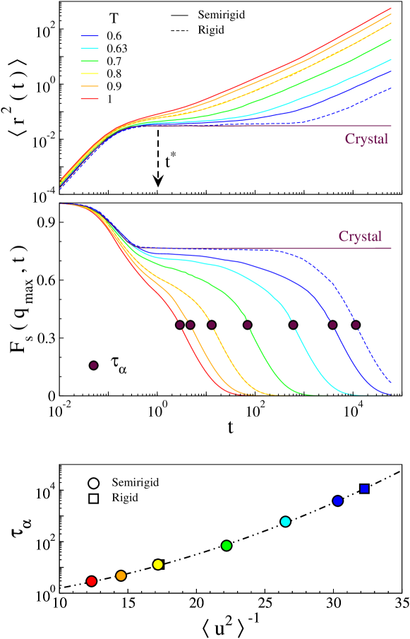
Figure 2: Monomer dynamics in the molecular liquid. As reference, a crystal state having the same density of the other states, obtained by spontaneous crystallization of an equilibrated liquid made of trimers with rigid bonds at $T=0.7$ is also plotted (maroon line). Top: MSD. The knee at about $t_{m}=0.175$ corresponds to the minimum of the velocity correlation function, see Fig.1. Middle: corresponding ISF curves. The long-time decay is stretched with stretching parameter $\beta\sim 0.6$. Bottom: scaling of the non-crystalline states on the universal master curve $\log\tau_{\alpha}$ vs $\langle u^{2}\rangle^{-1}$ (dot-dashed line) expressing the universal correlation between the fast vibrational dynamics and the slow relaxation Larini et al. (2008). $\langle u^{2}\rangle$ is the MSD evaluated at the time $t^{*}=1.023$ where $\log$ MSD vs. $\log t$ has the inflection point, see top panel. $t^{*}$ marks the end of the exploration of the cage by the trapped particle. The expression of the dot-dashed master curve is $\log\tau_{\alpha}=\alpha+\beta<u^{2}>^{-1}+\gamma<u^{2}>^{-2}$ with $\alpha=-0.424(1),\beta=2.7(1)\cdot 10^{-2},\gamma=3.41(3)\cdot 10^{-3}$ Larini et al. (2008).

III Results and discussion

We now present and discuss the results about our trimeric liquid. The states represent a significant set spanning a wide range of relaxation times. Below, it will be shown that they exhibit key features of the supercooled liquids, e.g. the stretching of the relaxation Larini et al. (2008); Ediger (2000); Ediger and Harrowell (2012), the presence of dynamical heterogeneity Larini et al. (2008); Ottochian et al. (2008); Ediger (2000); Ediger and Harrowell (2012), and all comply with the universal scaling between the cage rattling and the structural relaxation found in several glass-forming systems Larini et al. (2008); Ottochian et al. (2009); Puosi and Leporini (2011); Puosi et al. (2013); De Michele et al. (2011); Simmons et al. (2012); Pazmiño Betancourt et al. (2015); Ottochian and Leporini (2011a, b); Ottochian et al. (2013). From this respect, we believe that the conclusions to be drawn by their analysis are representative of supercooled molecular liquids broadly.

III.1 Transport and relaxation: general aspects

The cage effect is well evidenced by the velocity self-correlation function $C_{vv}(t)$ Hansen and McDonald (2006), which is shown in Fig.1. Initially, the decay is well accounted for by Eq.2. Later, a negative region develops due to backscattering from the cage wall leading, on average, to the reversal of the velocity of the particle. A minimum is seen at $t\sim t_{m}=0.175$. Superimposed to the slower decay faster oscillations are seen. By replacing the semirigid bond with a rigid one, they largely disappear, see Fig.1 (inset), so that they are ascribed to bond vibrations. Nonetheless, some oscillatory components are still present after the minimum. In atomic liquids, e.g. rubidium, similar components are due to sound waves that, owing to the low compressibility, reach wavelengths of a few particle diameters Hansen and McDonald (2006).

We define the monomer displacement in a time $t$ as:

$$\Delta\mathbf{r}_{i}(t)=\mathbf{r}_{i}(t)-\mathbf{r}_{i}(0)$$ (3)

where $\mathbf{r}_{i}(t)$ is the vector position of the $i$-th monomer at time $t$. The mean square displacement (MSD) $\langle r^{2}(t)\rangle$ is expressed as:

$$\langle r^{2}(t)\rangle=\left\langle\frac{1}{N}\sum_{i=1}^{N}\|\Delta\mathbf{r}_{i}(t)\|^{2}\right\rangle$$ (4)

where brackets denote the ensemble average. In addition to MSD the incoherent, self part of the intermediate scattering function (ISF) is also considered:

$$F_{s}(q,t)=\left\langle\frac{1}{N}\sum_{j=1}^{N}e^{i{\bf q}\cdot\Delta\mathbf{r}_{j}(t)}\right\rangle$$ (5)

ISF was evaluated at $q=q_{max}$, the maximum of the static structure factor ( $7.29\leq q_{max}\leq 7.35$ ).

Fig.2 shows MSD of the molecular monomers (top) and ISF (middle) curves of the states of interest. At very short times (ballistic regime) MSD increases according to $\langle r^{2}(t)\rangle\cong(3k_{B}T/m)t^{2}$ and ISF starts to decay. The repeated collisions slow the displacement of the tagged monomer, as evinced by the knee of MSD at $t\sim t_{m}=0.175$, i.e. very close to the minimum of the velocity correlation function, see Fig.1. At later times a quasi-plateau region, also found in ISF, occurs when the temperature is lowered. This signals the increased caging of the particle. Trapping is permanent in the crystalline state so that neither MSD nor ISF decay. In the other states, an inflection point is seen at $t^{*}=1.023$ in the log-log MSD plot, see Fig.2 (top). $t^{*}$ is state-independent in the present model Larini et al. (2008). The inflection point signals the end of the exploration of the cage by the trapped particle and the subsequent early escapes. The average escape time yields the structural relaxation time $\tau_{\alpha}$, defined by the relation $F_{s}(q_{max},\tau_{\alpha})=e^{-1}$. For $t>\tau_{\alpha}$ MSD increases more steeply and finally ends up in the diffusive regime, whereas ISF decays to zero as a stretched exponential with stretching parameter $\beta\sim 0.6$.

Fig.2 (bottom) shows that all the states under study (apart from the crystalline state) comply with the universal scaling between the fast vibrational dynamics and the slow relaxation in glass-forming systems, as expressed by the master curve between the mean square amplitude of the cage rattling $\langle u^{2}\rangle\equiv\langle r^{2}(t^{*})\rangle$ and the structural relaxation time $\tau_{\alpha}$ Larini et al. (2008); Ottochian et al. (2009); Puosi and Leporini (2011); Puosi et al. (2013); De Michele et al. (2011); Simmons et al. (2012); Pazmiño Betancourt et al. (2015); Ottochian and Leporini (2011a, b); Ottochian et al. (2013).

It is known Larini et al. (2008); Ottochian et al. (2008) that the mean square amplitude of the cage rattling $\langle u^{2}\rangle$ scales also the non-gaussian parameter $\alpha_{2}$, a measure of the non-gaussian character of the dynamics, and then of its heterogeneous character ($\alpha_{2}$ vanishes for gaussian, homogeneous dynamics) Ediger (2000). Scaling means that the maximum of the non-gaussian parameter $\alpha_{2}^{max}$ is a universal function of the structural relaxation time Larini et al. (2008); Ottochian et al. (2008). On this basis, given the structural relaxation time $\tau_{\alpha}$ of the states under study, we see that they range from states with virtually no dynamical heterogeneity, $\alpha_{2}^{max}\sim 0.2$, up to states with significant heterogeneity, $\alpha_{2}^{max}\sim 3.4$.

III.2 Inside the cage

We now turn our attention on how the cage rattling is affected by the cage shape. We correlate the direction of the monomer displacement $\hat{\bf u}_{i}(t)$ with the direction of the elongation of the VP surrounding the $i$-th particle at the initial time $t=0$. Fig.3 visualises the quantities of interest. The direction of the elongation is defined as Rahman (1966):

$$\hat{\bf u}^{C}_{i}=\frac{\mathbf{C}_{i}}{|\mathbf{C}_{i}|}$$ (6)

$\mathbf{C}_{i}$ is the position of the centroid, the center of mass of the VP vertices, with respect to the position of the $i$-th particle:

$$\mathbf{C}_{i}=\frac{1}{N_{v,\,i}}\sum_{j=1}^{N_{v,\,i}}\mathbf{v}^{j}_{i}$$ (7)

where $N_{v,\,i}$ and $\mathbf{v}^{j}_{i}$ are the number of vertices and the position of the VP $j$-th vertex with respect to the position of the $i$-th particle, respectively.

Figure 3: Quantities of interest to characterize the correlation between the displacement of the particle (green dot) and the cage shape. The magenta dot is the centroid of the vertices of the associated Voronoi polyhedron (VP) at the initial time, Eq.7. The highlighted regions are limited by planes perpendicular to $\mathbf{C}_{i}$ and passing through either the initial position of the particle or the centroid.

Figure 4: Local anisotropies of the cage rattling. Top: $\langle\cos\theta_{c}(t)\rangle$, Eq.8, at different temperatures. The unlabeled inset shows the complete decay. Bottom: $\langle\cos\theta_{p}(t)\rangle$, Eq.9. The dots mark the structural relaxation time $\tau_{\alpha}$. The left dashed line marks the minimum of the velocity correlation function at $t=t_{m}$, see Fig.1. The right dashed line marks the time needed by the trapped particle to explore the cage $t^{*}$, see Fig.2. Up to $t\sim 0.65$ $\langle\cos\theta_{p}(t)\rangle$ is nearly temperature-independent. The maximum of $\langle\cos\theta_{p}(t)\rangle$ signals that the particle, as in atomic systems Rahman (1966), tends initially to move to the centroid. The insets labelled as ”Rigid” plot the anisotropies for $T=0.6,0.9$ having replaced the semirigid bond with a rigid one and leaving any other parameter unchanged. They evidence that the oscillations in the time window $t_{m}\lesssim t\lesssim t^{*}$ of the main panels are due to the finite stiffness of the bond.

In order to investigate the correlation between the displacement of the trapped particle and the shape of the cage, we consider the time evolution of two distinct order parameters, namely the anisotropy of the particle displacement relative to the centroid with respect to the initial direction of the centroid, see Fig.3:

$$\langle\cos\theta_{c}(t)\rangle=\left\langle\frac{1}{N}\sum_{i=1}^{N}\frac{\big{[}\Delta\mathbf{r}_{i}(t)-\mathbf{C}_{i}\big{]}}{\big{|}\Delta\mathbf{r}_{i}(t)-\mathbf{C}_{i}\big{|}}\cdot\big{[}-\hat{\bf u}^{C}_{i}\big{]}\right\rangle$$ (8)

and the anisotropy of the particle displacement with respect to the initial direction of the centroid Rahman (1966), see Fig.3:

$$\langle\cos\theta_{p}(t)\rangle=\left\langle\frac{1}{N}\sum_{i=1}^{N}\hat{\bf u}_{i}(t)\cdot\hat{\bf u}^{C}_{i}\right\rangle$$ (9)

Complete isotropy yields $\langle\cos\theta_{i}\rangle=0$ ($i=p,c$). Perfect alignment of $\hat{\bf u}_{i}(t)$ with respect to $\hat{\bf u}^{C}_{i}$ yields $\langle\cos\theta_{p}\rangle=1$ whereas perfect alignment of $\big{[}\Delta\mathbf{r}_{i}(t)-\mathbf{C}_{i}\big{]}$ with respect to $-\hat{\bf u}^{C}_{i}$ yields $\langle\cos\theta_{c}\rangle=1$. Furthermore, if the monomer displacement is large with respect to $|\mathbf{C}_{i}|$, $\theta_{p}(t)\simeq\pi-\theta_{c}(t)$ and $\langle\cos\theta_{p}(t)\rangle\approx-\langle\cos\theta_{c}(t)\rangle$. The order parameters defined by Eq.8 and Eq.9 provide complementary information. By referring to Fig.3, positive values of $\langle\cos\theta_{c}(t)\rangle$ signal that the particle is preferentially located in regions I and II, whereas positive values of $\langle\cos\theta_{p}(t)\rangle$ denote preferential location of the particle in regions II and III.

Figure 5: Correlation plot of the asphericity and the volume of VPs of the melt of trimers at $T=1$ . No correlation is apparent.

Fig.4 (top) shows detailed plots of $\langle\cos\theta_{c}(t)\rangle$, Eq.8. At very short times the displacement $\Delta\mathbf{r}_{i}(t)$ is small and $\langle\cos\theta_{c}(t)\rangle\sim 1$. Then, the anisotropy drops in a temperature-independent way up to $t_{m}$, the time needed by most particles to reverse their initial velocity, see Fig.1. At later times the decay slows down and becomes temperature-dependent. The decay stops at about the structural relaxation time $\tau_{\alpha}$. At $t>\tau_{\alpha}$ a mild increase of $\langle\cos\theta_{c}(t)\rangle$ is observed to be followed by a later decay. The description of the non-monotonous relaxation of the order parameter in this viscoelastic regime goes beyond the purposes of the present paper and will be presented elsewhere.

Fig.4 (bottom) plots $\langle\cos\theta_{p}(t)\rangle$, Eq.9, at different temperatures. At very short times the direction of the particle displacement $\hat{\bf u}_{i}(t)$ is almost isotropic and $\langle\cos\theta_{p}(t)\rangle$ is small. Later, the particle approaches the initial position of the centroid of the VP vertices, $\langle\cos\theta_{p}(t)\rangle$ increases and reaches the maximum at $t_{m}$, when $C_{vv}(t)$ is at the minimum. The initial tendency of the trapped particle to move to the centroid has been reported Rahman (1966); Slotterback et al. (2008) and is clear indication that initially there is growing correlation between the local structure and the particle displacement. However, at later times the correlation decreases, up to $t\sim 0.65$ in an almost temperature-independent way. For $t\gtrsim 0.65$ the decrease of $\langle\cos\theta_{p}(t)\rangle$ is slowed down and becomes strongly temperature-dependent. The declining anisotropy $\langle\cos\theta_{p}(t)\rangle$, is consistent with our previous finding that the influence of both the size and the shape of the cage on the mean square displacement is lost within $t^{*}\sim 1$ Bernini et al. (2015a, b). For times longer than the structural relaxation time the escape from the cage reduces the order parameter further, and a negative tail is observed. The tail follows by the approximate relation $\langle\cos\theta_{p}(t)\rangle\approx-\langle\cos\theta_{c}(t)\rangle$, which holds at long times, and the positiveness of $\langle\cos\theta_{c}(t)\rangle$.

It seems proper to compare the decrease of the two order parameters in the range $t_{m}\lesssim t\lesssim t^{*}$ where structural relaxation is virtually missing Larini et al. (2008); Ottochian et al. (2009); Puosi and Leporini (2012b). First, by replacing the semirigid bond with a rigid one, one clarifies that the small oscillations which are superimposed to their decay in this time window are due to the finite stiffness of the bonds, see Fig.4 (insets). One also notices that, differently from $\langle\cos\theta_{c}(t)\rangle$, $\langle\cos\theta_{p}(t)\rangle$ is largely temperature-independent if $t\lesssim 0.65$, see Fig.4. This is due to the different character of the two order parameters. The time-dependence of $\langle\cos\theta_{p}(t)\rangle$ around its maximum at $t_{m}$ tracks the bounce of the particle with the cage wall. This process is nearly temperature-independent, see Fig.1. Instead, the anisotropy $\langle\cos\theta_{c}(t)\rangle$ decreases if the population of particles, initially located in regions I and II of Fig.3, displaces appreciably to region III. The same process affects $\langle\cos\theta_{p}(t)\rangle$ less because region III may be reached from region II also with no change of $\theta_{p}$. To reach the region III the particle initially approaches the centroid of the VP vertices, located close to the voids between the particles marking the weak spots of the cage. The approach to the centroid, and then the decay of $\langle\cos\theta_{c}(t)\rangle$, is limited by the softness of the cage Dyre (2006); Starr et al. (2002); Puosi and Leporini (2012b, 2015), which is temperature-dependent. The elastic response by the cage will be dealt with in Sec.III.3.2.

The above discussion suggests that $\langle\cos\theta_{p}(t)\rangle$ tracks the monomers being backscattered by the cage wall, whereas $\langle\cos\theta_{c}(t)\rangle$ is more sensitive to the monomers escaping from the cage. This picture is reinforced by observing the changes of the two anisotropies around $t^{*}$. We remind that at $t^{*}$ early breakouts from the cage start to take place, see Fig.2 and Sec.III.1 Larini et al. (2008); Ottochian et al. (2009). $\langle\cos\theta_{p}(t)\rangle$ has an inflection point at $t^{*}$ which develops in $\langle\cos\theta_{c}(t)\rangle$ only at the lowest temperature, see Fig.4. The accelerated decay of $\langle\cos\theta_{c}(t)\rangle$ around $t^{*}$ suggests that $\langle\cos\theta_{c}(t)\rangle$ is more affected by the monomers leaving the cage, since they lose correlation with the cage geometry, whereas $\langle\cos\theta_{p}(t)\rangle$ is more sensitive to the trapped particles which keep on being affected by the cage geometry. At low temperature, being the escapes quite rare, the two anisotropies are more similar.

Figure 6: Correlation plot of the surface and the volume of VPs of the melt of trimers at $T=1$ (Pearson correlation coefficient $r=0.973$). The lines are Eq.11 with the indicated values of the asphericity. The best-fit value of the asphericity ($a=0.404$) compares well with the average asphericity of the VPs ($\langle a\rangle=0.405$).

Figure 7: Selected time-frame of the surface (top), volume (middle) and asphericity (bottom) of the VP surrounding particular central (green) and end (magenta) monomers of different trimers of the melt at $T=1$. Note the extreme similarity of the fluctuations of the volume and the surface and the different character of the ones of the asphericity.

III.3 Cage border

Sec.III.2 discussed how the cage rattling of the trapped monomers is affected by the neighbours. Here, we reverse the point of view and investigate how the neighbours are affected by the collisions of the trapped monomer. To this aim, we consider the geometry of the cage in terms of the volume $V_{i}$, the surface $S_{i}$ and the asphericity $a_{i}$ of the $i$-th VP. The asphericity is defined as:

$$a_{i}=\frac{S_{i}^{3}}{36\pi V_{i}^{2}}-1$$ (10)

It is non-negative and vanishes for a sphere. For the system under study $a\sim 0.35-0.45$, namely the VPs are moderately non-spherical (the asphericities of the dodecahedron and the octahedron are $0.325$ and $0.654$, respectively ) Bernini et al. (2015b, a). Since each VP includes one particle only, the VP volume is a measure of the local density.

III.3.1 Statics: volume-surface correlations

There are no correlations between the asphericity and the volume. Fig.5 shows a representative example. No correlations are also found between the asphericity and the surface of the VPs (not shown). Instead, Fig.6 evidences the strong correlation between the surface and the volume of VPs. It follows from the good packing and the subsequent relatively narrow width of the distribution of the asphericity Bernini et al. (2015b, a). To show that we recast Eq.10 as

$$S=\Big{[}36\,\pi\,(a+1)\Big{]}^{1/3}\,V^{2/3}$$ (11)

Then, we neglect the fluctuations of the asphericity $a$ and treat it as an adjustable parameter to best-fit Eq. 11 to the correlation plot. The result is superimposed to the numerical data in Fig.6. It provides a nice fit with best-fit asphericity rather close to the average asphericity of the VPs of the state under consideration. The plot also shows that the cloud of data is bounded within the approximate range of the asphericity, $a\sim 0.35-0.45$, see Fig.5.

III.3.2 Dynamics: elastic response

Volume, surface and asphericity of the $i$-th VP fluctuate around their average values due to the rearrangement of both the tagged $i$-th particle and the surroundings.

To give clear impression of the surface-volume correlations we plot in Fig.7 a selected time-frame of the fluctuations of volume, surface and asphericity of the VP surrounding two specific central and end monomers. The strong correlation of the volume and the surface is quite apparent. Differently, the fluctuations of the asphericity has poor resemblance with the ones of the volume and surface.

To characterize in a quantitative way the fluctuations we define the correlation function:

$$C_{x}(t)=\left\langle\frac{\sum\limits_{i=1}^{N}\Big{[}x_{i}(t)-\langle\langle x\rangle\rangle\Big{]}\Big{[}x_{i}(0)-\langle\langle x\rangle\rangle\Big{]}-\delta_{x}}{\sum\limits_{i=1}^{N}\Big{[}x_{i}(0)-\langle\langle x\rangle\rangle\Big{]}^{2}-\delta_{x}}\right\rangle$$ (12)

with $x=V,S,a$. $\langle\langle x\rangle\rangle$ denotes the average of $x$ over all the $N$ monomers. Eq.12 yields $C_{x}(0)=1$. To ensure that $C_{x}(t)$ vanishes at long times we set

$$\delta_{x}=\frac{N_{c}N_{e}}{N}\Big{[}\langle\langle x\rangle\rangle_{c}-\langle\langle x\rangle\rangle_{e}\Big{]}^{2}$$ (13)

where $\langle\langle x\rangle\rangle_{c}$ and $\langle\langle x\rangle\rangle_{e}$ are the average of $x$ restricted to the $N_{c}$ central and the $N_{e}$ end monomers, respectively ($N_{c}+N_{e}=N$). Eq.13 is derived in Appendix A.

Figure 8: Correlation functions, Eq.12, of volume (top), surface (middle) and asphericity (bottom) of VPs at different temperatures. The dashed lines mark the region $t_{m}\leq t\leq t^{*}$ as in Fig. 1 and Fig. 4. Insets: magnification of the oscillatory behavior at intermediate times. The insets labelled as ”Rigid” plot the correlation function for $T=0.6,0.9$ having replaced the semirigid bond with a rigid one and leaving any other parameter unchanged. They evidence that the oscillations are not due to the finite stiffness of the bond but to the elastic response of the local structure.

Fig.8 shows $C_{x}(t)$ with $x=V$ (top panel), $S$ (middle panel) and $a$ (bottom panel) at different temperatures. As anticipated, there is strong similarity between $C_{V}(t)$ and $C_{S}(t)$. Within the time $t_{m}$ needed by most particles to reverse their initial velocity, a large part of the correlations of the cage geometry is lost. For $t\gtrsim t_{m}=0.175$, the decay becomes extremely slow and strongly dependent on the temperature. This parallels the time dependence of the order parameter $\langle\cos\theta_{c}(t)\rangle$, see Fig.4 (top). At long times, the structural relaxation erases the residual correlations of the cage geometry and $C_{x}(\tau_{\alpha})\simeq 0.1$, $x=V,S,a$.

We now address the fluctuation correlation in the time window $t_{m}\lesssim t\lesssim t^{*}$ where both the velocity correlations, Fig.1, and the order parameters, Fig.4, hint at the elastic response of the cage to the colliding trapped particle. The insets of Fig.8 focus on this time interval. Correlation oscillations in VP size, but not in shape, are apparent. The oscillations are still present if one replaces the semirigid bonds by rigid bonds (see insets labelled as ”Rigid” in Fig.8), proving that they are not due to bond vibrations. We interpret the minimum of $C_{V}(t)$ and $C_{S}(t)$ as due to the deformation of the local structure following the disordering collision of the central particle with the cage, whereas the successive maximum and the later smaller oscillations reflect the elastic response to recover the original arrangement. This sort of collective ”cage ringing” is not tracked by the asphericity, see Fig.8 (bottom), confirming the poor correlation between the size and the shape of the cage. It is worth noting that the elastic effects seen via the VP volume and surface are small, in that the fluctuations of the VP size and shape are quite limited in size, as seen by Fig.5 and Fig.6.

III.4 Beyond the cage border

Sec.III.2 and Sec.III.3 investigated the cage rattling and the effects on the closest neighbours, respectively. Here, we complete the analysis and extend the range of the neighbours. It will be now shown that in a time about $t_{m}=0.175$, needed by most particles to bounce back from the cage wall (Fig.1), extended modes involving particles beyond the first shell appear. The modes have solid-like character since $\tau_{\alpha}\gg 1$ Larini et al. (2008); Ottochian et al. (2009); Puosi and Leporini (2012b), i.e. they are distinct in nature from the hydrodynamic modes developed by the drag force of a moving particle Alder and Wainwright (1970). We divide the discussion in two parts by first describing the onset of extended displacement correlations for $t\leq t^{*}$, when the trapped particle completes the cage exploration, and then their persistence and decay for $t>t^{*}$. In particular, in Sec. III.4.1 we will compare the influence of the extended modes on the moves of the trapped particle in a time $t^{*}$ with the one of the local geometry. Sec.III.2 noted that the influence of the cage shape at $t^{*}$ is smaller than at $t_{m}$.

III.4.1 Onset of the displacement correlations ($t\leq t^{*}$)

To reveal the modes, we characterize the degree of correlation between the direction of the displacements performed simultaneously in the same lapse of time $t$ by two particles initially spaced by $r_{ij}$ via the space correlation function Puosi and Leporini (2012c); Puosi and Leporini (2013):

$$C_{\bf{u}}(r,t)=\left\langle\frac{1}{N}\sum_{\begin{subarray}{c}i=1\end{subarray}}^{N}\hat{\bf u}_{i}(t)\cdot{\bf{U}}_{i}(r,t)\right\rangle$$ (14)

with:

$${\bf{U}}_{i}(r,t)=\frac{1}{N(r)}\sum_{\begin{subarray}{c}j=1\\ i\neq j\end{subarray}}^{N}\hat{\bf u}_{j}(t)\delta(r-r_{ij})$$ (15)

where $\hat{\bf u}_{i}(t)$ and $N(r)$ are the direction of $\Delta\mathbf{r}_{i}(t)$, Eq.3, and the average number of particles initially spaced by $r$, respectively. If the displacements are perfectly correlated in direction, one finds $C_{\bf{u}}(r,t)=1$. $C_{\bf{u}}(r,t)$ has some formal similarity with $\langle\cos\theta_{p}(t)\rangle$, Eq.9, but the two quantities are quite different:

• $\langle\cos\theta_{p}(t)\rangle$ is a measure of the directional correlation of the displacement performed in a time $t$ by the tagged particle and the axis $\hat{\bf u}^{C}_{i}$ set by the initial cage geometry.

• $C_{\bf{u}}(r,t)$ is a measure of the average directional correlation of the simultaneous displacements performed in a time $t$ between the tagged particle and each of the surrounding particles at distance $r$.

Fig.9 (top) plots the spatial distribution of the correlations for different times $t$. It is seen that if the time is shorter than $t_{m}=0.175$, the time needed by most particles to reverse their initial velocity due to backscattering, the correlations are limited to the bonded particles at $r=r_{b}=b$ and, weakly, the first shell (Fig.9, lower panels). For longer times, the correlation grows in both magnitude and spatial extension with characteristic peaks corresponding to the different neighbour shells Puosi and Leporini (2012c); Puosi and Leporini (2013). These spatial directional correlations have been also observed in simulations on hard spheres and hard disks Doliwa and Heuer (2000) and experiments on colloids Weeks et al. (2007). Fig.9 (lower panels) shows that the onset of the correlations of both the third and the fourth shells is delayed of about $0.4$ time units due to the finite propagation speed of the perturbation. It is also seen that the growth of the correlation levels off at times $\sim t^{*}$ and is temperature-independent, whereas their magnitude weakly decreases with the temperature. The limited influence of the temperature mirrors the one of the velocity correlation loss in the intermediate range $t_{m}\lesssim t\lesssim t^{*}$.

Comparing $\langle\cos\theta_{p}(t)\rangle$, Fig.4, and $C_{\bf{u}}(r,t)$, Fig.9, leads to a clearer picture of how the particle in the cage progresses between $t_{m}$ and $t^{*}$. Before $t_{m}$ the cage geometry has increasing, even if weak, influence, see Fig.4. After $t_{m}$, the displacement-displacement correlations increase and extend in space, Fig.9, with parallel decrease of the influence of the cage geometry, Fig.4. At the completion of the cage exploration at $t^{*}$, the anisotropy of the particle displacement due to local order is small and declining, whereas the displacement-displacement correlations reach their maximum. The picture provides an interpretation of the puzzling finding that for a given state of a liquid of linear chains (trimers or decamers), the end and the central monomers, which have different distributions of the cage size and shape, have equal $\langle r^{2}(t^{*})\rangle\equiv\langle u^{2}\rangle$ Bernini et al. (2015b). On one hand, that finding exposes the minor role of the cage geometry. On the other hand, it is well explained by the extended displacement-displacement correlations evidenced in Fig.9, overriding the different local order of the end and the central monomers. The leading role of the extended displacement-displacement correlations in setting the monomer moves on the time scale $t^{*}$ is proven by the fact that physical states with identical spatial distributions of the displacement-displacement correlations exhibit equal mean square amplitude of the cage rattling $\langle r^{2}(t^{*})\rangle\equiv\langle u^{2}\rangle$ Puosi and Leporini (2012c); Puosi and Leporini (2013). The coupling between the rattling process and extended modes has been indicated Widmer-Cooper et al. (2008, 2009); Karmakar et al. (2016); Wyart (2010).

Figure 9: Top panel: spatial distribution $C_{\bf{u}}(r,t)$ of the correlations between the simultaneous displacements of the central particle and the surrounding particles at distance $r$ for different times $t$ and $T=0.6$. The time window starts at $t=0.1<t_{m}=0.175$ and ends at $t^{*}=1.023$. The peak positions correspond nearly to the ones of the radial distribution function Puosi and Leporini (2012c); Puosi and Leporini (2013). At constant density they do not depend on the temperature. Bottom panels: onset of the correlations at the peak positions at $T=0.6$ (left) and $T=1$ (right). $r_{b}=b$ equals the bond length distance.

Displacement correlations have been evidenced in an experimental study of a dense colloidal suspension Weeks et al. (2007). Contact with our simulations is allowed by splitting the displacement direction in the transverse and the longitudinal components with respect to the direction of the separation vector:

$$u_{m}^{L} = \hat{\bf u}_{m}\cdot\hat{\bf r}_{ij}$$ (16)

$$u_{m}^{T} = \hat{\bf u}_{m}-u_{m}^{L}\hat{\bf r}_{ij}$$ (17)

where $m=i,j$ and $\hat{\bf r}_{ij}\equiv({\bf r}_{j}-{\bf r}_{i})/r_{ij}$ refers to the initial configuration before the displacement occurs. Let us define the related correlation functions as:

$$C_{L}(r,t)=\left\langle\frac{1}{N\;N(r)}\sum_{\begin{subarray}{c}i,j=1\\ i\neq j\end{subarray}}^{N}u_{i}^{L}(t)\cdot u_{j}^{L}(t)\delta(r-r_{ij})\right\rangle$$ (18)

$$C_{T}(r,t)=\left\langle\frac{1}{N\;N(r)}\sum_{\begin{subarray}{c}i,j=1\\ i\neq j\end{subarray}}^{N}u_{i}^{T}(t)\cdot u_{j}^{T}(t)\delta(r-r_{ij})\right\rangle$$ (19)

The longitudinal and the transverse components are related to the total correlation function by:

$$C_{\bf{u}}(r,t)=C_{L}(r,t)+C_{T}(r,t).$$ (20)

Fig.10 plots $C_{L}(r,t)$ (top) and $C_{T}(r,t)$ (middle). The longitudinal correlations increase faster than the transverse ones with increasing time $t$. This is seen in Fig.10 (bottom) plotting for selected positions the growth function:

$$\widetilde{C}_{X}(r,t)=\frac{C_{X}(r,t)-C_{X}(r,0.1)}{C_{X}(r,t^{*})}\,,\hskip 14.22636ptX\in\{L,T\}$$ (21)

The longitudinal correlations have different spatial distribution with respect to the transverse ones. Fig.10 proves that the bonded particles ( $r=0.97$) are correlated mostly via their longitudinal displacements. Fig.10 also shows that the oscillatory character of the total displacement correlation function is largely due to the longitudinal component, whereas the transverse component is much less sensitive to the radial density distribution. Other salient features are the negative minimum of $C_{L}(r,t)$ at $r\simeq 1.4$, corresponding to the first minimum of $g(r)$, and the pronounced maximum of $C_{T}(r,t)$ close to the same position. All these hallmarks have been observed in an experimental study of a dense colloidal suspension Weeks et al. (2007). This suggests that the key features of the displacement correlations are not strictly affected by the molecular connectivity.

Figure 10: Spatial distribution of the correlations between the simultaneous longitudinal (top), Eq.18, and tranverse (middle), Eq.19, components of the displacements of the central particle and the surrounding particles at distance $r$ for different times $t$ and $T=0.6$. The time window starts at $t=0.1<t_{m}=0.175$ and ends at $t^{*}=1.023$. The lower panel plots the growth of the correlation, Eq.21, at selected positions. The longitudinal correlations increase faster than the transverse ones.

Figure 11: Spatial distribution of the correlations between the simultaneous overall (top), Eq.14, longitudinal (middle), Eq.18, and tranverse (bottom), Eq.19, components of the displacements of the central particle and the surrounding particles at distance $r$ for different times $t\geq t^{*}=1.023$ and $T=1$. At the selected temperature $\tau_{\alpha}=3$ and the average molecular reorientation time $\tau_{ee}=126$ Ottochian et al. (2009).

Even if the full interpretation of the spatial pattern of $C_{L}(r,t)$ and $C_{T}(r,t)$ is deferred to future work, some preliminary remarks may be offered. The negative dip of $C_{L}(r,t)$ at $r\simeq 1.4$ close to the maximum of $C_{T}(r,t)$ is consistent with particles approaching , or receding from, each other in a compression/dilation motion while transversely displacing the same way. The role of quasi-linear arrangements of particles was suggested in regard to the oscillatory behaviour of the longitudinal correlation of the displacements Weeks et al. (2007). From this respect, evidence of bond-bond alignment, i.e. three monomers in a row, is reported for the molecular liquid under study Bernini et al. (2013). Moreover, in densely packed colloids it is known that straight paths of $\ell_{SP}$ particles are exponentially distributed as $\sim\exp[-\ell_{SP}/\bar{\ell}_{SP}]$ with $\bar{\ell}_{SP}\sim 0.73,0.87$ depending on the sample preparation Schenker et al. (2008). Interestingly, the height of the peaks of $C_{\bf{u}}(r,t)$, due to the longitudinal component, decay exponentially with distance as $\sim\exp[-r/\xi]$ with $0.7\leq\xi\leq 1$ Puosi and Leporini (2012c); Puosi and Leporini (2013), suggesting a connection with the distribution of the length of aligned particles.

We briefly discuss the weak negative tail observed in $C_{T}(r,t)$ at large $r$, Fig.10 (middle), affecting $C_{\bf{u}}(r,t)$, Fig.9. The tail disappears by increasing the size of the system (not shown) and is due to the momentum conservation requiring that, with fixed center of mass of the system, a displacement of one particle induces correlated counter-displacements on the other ones. The size effect does not affect the longitudinal displacements when averaged over the sphere with radius $r$, see Fig.10 (top). This may be understood by reminding that the direction of the displacement of the central particle sets the sphere axis. Then, the larger size effect on the transverse displacement follows from the larger weight of the equatorial belt in the average with respect to the polar zones, so that the induced counter-displacements contribute negative terms to $C_{T}(r,t)$ and negligibly to the average of $C_{L}(r,t)$.

Figure 12: Time dependence of the overall, longitudinal and transverse correlations at the indicated positions in Fig.11. At the selected temperature $\tau_{\alpha}=3$ and the average molecular reorientation time $\tau_{ee}=126$ Ottochian et al. (2009). The time window starts before $t_{m}=0.175$. Note the maximum at about $t^{*}=1.023$.

III.4.2 Persistence and decay of the displacement correlations ($t>t^{*}$)

What happens at the displacement correlations for longer sampling times $t>t^{*}=1.023$ ? We already know that small changes are observed up to $t=\tau_{\alpha}$ even for sluggish states, thus creating a plateau region on increasing $t$ Puosi and Leporini (2012c); Puosi and Leporini (2013). In this range the presence of quasi-static collective elastic fluctuations Puosi and Leporini (2012b) set the magnitude of the direction correlations. A view of the displacement correlations in space for $t>t^{*}$ is given in Fig.11. The complete view of the growth, up to $t\sim t^{*}$, the plateau region up to $t\sim\tau_{\alpha}$, and the following decay is presented in Fig.12. Note that, since the decay is quite slow, in order to visualise all the time range, a state with short structural relaxation ($\tau_{\alpha}=3$) is considered, thus limiting the persistence of the maximum longitudinal and transverse correlations. Fig.11 shows that the spatial modulation of both the longitudinal and the transverse correlations are averaged for $t>\tau_{\alpha}$. At longer sampling times the magnitude of the correlations decreases further. From this respect, an important time scale is the average molecular reorientation time $\tau_{ee}$, defined as $C_{ee}(\tau_{ee})=1/e$ where $C_{ee}(t)$ is the end-to-end time correlation function Ottochian et al. (2009). The correlations vanish for $r\gtrsim 2$ and $t\gg\tau_{ee}$. Nonetheless, some permanent correlations are left at shorter distances. In particular, residual correlations due to the intrachain connectivity are present for $1\lesssim r\lesssim 2$, together with large correlations between bonded monomers at $r\simeq 0.97$. Thus, we see that the connectivity of the trimer does not affect the correlation of the displacements of monomers spaced of more than two diameters.

IV Conclusions

The present paper investigates by MD simulations of a dense molecular liquid the key aspects driving the moves of the monomers in the cage of the surrounding ones. The aim is clarifying if the displacements are driven by the local geometry of the cage or the solid-like extended modes excited by the monomer-monomer collisions. The main motivations reside in both contributing to the intense ongoing research on the relation between the vibrational dynamics and the relaxation in glassfoming systems, and improving our microscopic understanding of the universal correlation between the relaxation and the mean-square amplitude of the rattling in the cage, $\langle u^{2}\rangle$, a quantity related to the Debye-Waller factor.

To discriminate between the roles of the local geometry and the collective extended modes in the single-particle vibrational dynamics, the cage rattling is examined on different length scales. First, the anisotropy of the rattling process due to local order, i.e. the arrangement of the first shell, is characterized by two order parameters sensing the monomers succeeding or failing to escape from the cage. Then, the collective response of the surroundings excited by the monomer-monomer collisions is considered. The collective response is initially restricted to the nearest neighbours of the colliding particle by investigating statics and fluctuations of the VP surface, volume and asphericity. Then, the long-range excitation of the farthest neighbours is scrutinised by searching spatially-extended correlations between the simultaneous fast displacements of the caged particle and the surroundings.

Two characteristic times are found: $t_{m}=0.175$ and $t^{*}\sim 1$. The former is the time when the velocity correlation function reaches the minimum. The latter is the time needed by the trapped particle to explore the cage with mean square rattling amplitude $\langle u^{2}\rangle$. One finds that the anisotropy of the random walk driven by the local order develops up $t_{m}$, then decreases and becomes small at $t^{*}\sim 1$. On the other hand, between $t_{m}$ and $t^{*}$ the monomer-monomer collisions excite both the elastic response of the cage and the long-range collective modes of the surroundings in parallel to the decreasing role of the local anisotropies. The longitudinal component of the long-range collective modes has stronger spatial modulation than the transverse one with wavelength of about the particle diameter, in close resemblance with experimental findings on colloids.

All in all, we conclude that the monomer dynamics at $t^{*}$, and then $\langle u^{2}\rangle$, is largely affected by solid-like extended modes and not the local geometry, in harmony with previous findings Puosi and Leporini (2012c); Puosi and Leporini (2013, 2012b, 2015); Bernini et al. (2015a, b), in particular reporting strong, universal correlations with the elasticity Puosi and Leporini (2012b, 2015), and poor correlation with the size and the shape of the cage Bernini et al. (2015a, b). On a more general ground, our study suggests, in close contact with others Widmer-Cooper et al. (2008, 2009); Karmakar et al. (2016); Wyart (2010), that the link between the fast dynamics and the slow relaxation is rooted in the presence of modes extending farther than the first shell.

Appendix A Derivation of $\delta_{x}$, Eq.13

Let us define the auxiliary quantity:

$$X(t)=\sum_{i=1}^{N}\Big{[}x_{i}(t)-\langle\langle x\rangle\rangle\Big{]}\Big{[}x_{i}(0)-\langle\langle x\rangle\rangle\Big{]}$$ (22)

$$=\sum_{j=1}^{N_{c}}\Big{[}\big{(}x_{j}(t)-\langle\langle x\rangle\rangle\big{)}\big{(}x_{j}(0)-\langle\langle x\rangle\rangle\big{)}\Big{]}$$ (23)

$$+\sum_{h=1}^{N_{e}}\Big{[}\big{(}x_{h}(t)-\langle\langle x\rangle\rangle\big{)}\big{(}x_{h}(0)-\langle\langle x\rangle\rangle\big{)}\Big{]}$$

$\langle\langle x\rangle\rangle$ denotes the average of $x$ over all the $N$ monomers. Let us define $\langle\langle x\rangle\rangle_{c}$ and $\langle\langle x\rangle\rangle_{e}$ as the averages of $x$ restricted to the $N_{c}$ central and the $N_{e}$ end monomers, respectively ($N_{c}+N_{e}=N$). The average $\langle\langle x\rangle\rangle$ is related to $\langle\langle x\rangle\rangle_{c}$ and $\langle\langle x\rangle\rangle_{e}$ by the equation:

$$\langle\langle x\rangle\rangle=\frac{N_{c}}{N}\langle\langle x\rangle\rangle_{c}+\frac{N_{e}}{N}\langle\langle x\rangle\rangle_{e}$$ (24)

In Eq.23 we add and subtract $\langle\langle x\rangle\rangle_{c}$ to $x_{j}(t)$, and do the same to $x_{j}(0)$. Also, we add and subtract $\langle\langle x\rangle\rangle_{e}$ to $x_{h}(t)$ and do the same to $x_{h}(0)$. If $t\to\infty$ the fluctuations of $(x_{j}(t)-\langle\langle x\rangle\rangle_{c})$ and the fluctuations of $(x_{j}(0)-\langle\langle x\rangle\rangle_{c})$ have both zero average and are uncorrelated. Analogously for the fluctuations of $(x_{h}(t)-\langle\langle x\rangle\rangle_{e})$ and the fluctuations of $(x_{h}(0)-\langle\langle x\rangle\rangle_{e})$. Then, we yield

$$\delta_{x} \equiv \lim_{t\to\infty}X(t)$$ (25)

$$= N_{c}\Big{[}\langle\langle x\rangle\rangle_{c}-\langle\langle x\rangle\rangle\Big{]}^{2}+N_{e}\Big{[}\langle\langle x\rangle\rangle_{e}-\langle\langle x\rangle\rangle\Big{]}^{2}$$ (26)

Plugging Eq.24 into Eq.26 yields :

$$\delta_{x} = N_{c}\left[\frac{N_{e}}{N}\langle\langle x\rangle\rangle_{c}-\frac{N_{e}}{N}\langle\langle x\rangle\rangle_{e}\right]^{2}+$$ (27)

$$+ N_{e}\left[\frac{N_{c}}{N}\langle\langle x\rangle\rangle_{c}-\frac{N_{c}}{N}\langle\langle x\rangle\rangle_{e}\right]^{2}$$

$$= \frac{N_{c}N_{e}}{N}\Big{[}\langle\langle x\rangle\rangle_{c}-\langle\langle x\rangle\rangle_{e}\Big{]}^{2}$$

Eq.27 coincides with Eq.13.

Appendix B On the presence of a crystalline fraction

Since the model with rigid bonds exhibits weak crystallization resistance, we have paid particular attention to detect any crystallization signature. From this respect, we have monitored some key quantities under equilibration and production of both the rigid and semirigid systems. We summarize the results:

i) the radial distribution function compares rather well with the one of atomic liquids, apart from the extra-peak due to the bonded monomers.

ii) the pressure and the configurational energy exhibit neither drops nor even slow decreases within 1 %, during the runs.

iii) no global order and even microcrystalline domains are seen by visual inspection of the samples. Note that, if the sample crystallizes, ordering is strikingly visible, e.g. see Fig. 10 of ref.Bernini et al. (2013).

iv) no order revealed by Steinhard global order parameters Bernini et al. (2013).

v) the mean square displacement always increases steadily with time. In a crystalline sample it levels off, see Fig.2 (top).

vi) full decorrelation of the incoherent part of the intermediate scattering function in both equilibration and production runs in all cases except the production runs of the system with rigid bonds at $T=0.6$. In the presence of a solid-like fraction the incoherent part of the intermediate scattering function decays to a finite plateau at long times, see Fig.2 (middle).

It is worth noting that the crystalline state obtained by spontaneous crystallization of an equilibrated liquid made of trimers with rigid bonds at $T=0.7$ considered in Fig.2 does not pass any of the above tests.

The tests iv), v) and vi) are now discussed in detail.

B.0.1 Test iv): absence of long-range order

To characterize the degree of global positional ordering of our samples we resort to the metric $Q_{l,global}$ Steinhardt et al. (1983); Bernini et al. (2013). To this aim, one considers in a given coordinate system the polar and azimuthal angles $\theta({\bf r}_{ij})$ and $\phi({\bf r}_{ij})$ of the vector ${\bf r}_{ij}$ joining the $i$-th central monomer with the $j$-th one belonging to the neighbors within a preset cutoff distance $r^{*}=1.2\;\sigma^{*}\simeq 1.35$ Steinhardt et al. (1983). The vector ${\bf r}_{ij}$ is usually referred to as a ”bond” and has not to be confused with the actual chemical bonds of the polymeric chain!

To define a global measure of the order in the system, one calculates the quantity Steinhardt et al. (1983):

$$\bar{Q}_{lm}^{global}=\frac{1}{N_{b}}\sum_{i=1}^{N}\sum_{j=1}^{n_{b}(i)}Y_{lm}\Big{[}\theta({\bf r}_{ij}),\phi({\bf r}_{ij})\Big{]}$$ (28)

where $n_{b}(i)$ is the number of bonds of $i$-th particle, $N$ is the total number of particles in the system, $Y_{lm}$ denotes a spherical harmonic and $N_{b}$ is the total number of bonds i.e:

$$N_{b}=\sum_{i=1}^{N}n_{b}(i)$$ (29)

The global orientational order parameter $Q_{l,global}$ is defined by the rotationally invariant combination:

$$Q_{l,global}=\left\langle\left[\frac{4\pi}{(2l+1)}\sum_{m=-l}^{l}|\bar{Q}_{lm}^{global}|^{2}\right]^{1/2}\right\rangle$$ (30)

In the absence of global ordering $Q_{l,global}=0$ in systems with infinite size. In the presence of long-range crystalline order $Q_{l,global}\neq 0$ , e.g. $Q_{6,global}\sim 0.5$ Steinhardt et al. (1983); Bernini et al. (2013), with exact values depending on the kind of order. Fig.13 shows $Q_{6,global}$ vs. $Q_{4,global}$ for all the states under investigation. They are compared with one typical crystalline state of the system with rigid bonds. Other crystalline states yield $Q_{4,global}$-$Q_{6,global}$ pairs within the size of the diamond. The non-ideal values of the order parameters of the crystalline state indicate imperfect long-range ordering Steinhardt et al. (1983); Bernini et al. (2013). We were unable to crystallize the system with semirigid bonds which, however, having $b=b_{rigid}$, is anticipated to have order parameters similar to the rigid bond case. Fig.13 shows that only the crystalline state has global, long-range order.

Figure 13: Global order parameters $Q_{6,global}$ and $Q_{4,global}$. The crystal state is the same considered in Fig.2 and is the only state exhibiting global order.

B.0.2 Tests v) and vi): absence of cristalline fractions

Fig.2 shows that if the sample crystallizes the changes of both MSD and ISF stop. In principle, the MSD increase in time may be also seen if supercooled liquids and crystalline fraction coexist Zhang et al. (2009). In this heterogeneous case the overall MSD is largely contributed by the mobile phase, since the MSD of the arrested phase levels off rapidly. However, ISF would reach a plateau at long times due to the frozen phase unable to lose the position correlation tracked by ISF. Fig.2 shows that ISF vanishes at long times in all states, except one to be discussed below, ruling out the presence of polycrystallinity at the end of the production runs, i.e. no crystalline regions formed during the equilibration and the subsequent production runs. The ISF of the system with rigid bonds at $T=0.6$ is still non-zero at the end of the production runs (due to our decision to stop the simulation soon after $\tau_{\alpha}$). To get a rough estimate of the maximum crystalline fraction $\phi_{c}^{max}$, we identify $\phi_{c}^{max}$ with the ratio of the residual ISF height, $ISF_{r}$, with the ISF plateau of the crystal state, $ISF_{c}$, (weakly dependent on T). We get $\phi_{c}\leq\phi_{c}^{max}=ISF_{r}/ISF_{c}\simeq 0.09$. We offer arguments to conclude that the possible crystalline fraction of the system with rigid bonds at $T=0.6$, if present, is much less than the upper limit $\phi_{c}^{max}$, and, in any case, plays negligible role. In fact:
1) the system with rigid bonds at $T=0.6$ passes the tests i), ii), iii), iv), v);
2) the same system at $T=0.9$, where no crystalline fraction is present, provides quite close, or even coincident, results to the ones gathered at $T=0.6$, see the insets of Fig.1, Fig.4, Fig.8. Note also that the results of the systems with rigid and non-rigid bonds are also quite close, see Fig.1 and Fig.8;
3) the cage rattling amplitude and the structural relaxation of the system with rigid bonds at $T=0.6$ fulfill the universal scaling between the fast vibrational dynamics and the slow relaxation in glass-forming systems, see Fig.2 (bottom) and Sec.III.1 Larini et al. (2008); Ottochian et al. (2009); Puosi and Leporini (2011); Puosi et al. (2013); De Michele et al. (2011); Simmons et al. (2012); Pazmiño Betancourt et al. (2015); Ottochian and Leporini (2011a, b); Ottochian et al. (2013). The universal scaling is anticipated to fail in semicrystalline materials where the frozen component has finite rattling amplitude but no relaxation.

References

- Hansen and McDonald (2006) J. P. Hansen and I. R. McDonald, Theory of Simple Liquids, 3rd Ed. (Academic Press, 2006).
- Götze (2008) W. Götze, Complex Dynamics of Glass-Forming Liquids: A Mode-Coupling Theory (Oxford University Press, Oxford, 2008).
- Berthier and Biroli (2011) L. Berthier and G. Biroli, Rev. Mod. Phys. 83, 587 (2011).
- Ediger and Harrowell (2012) M. D. Ediger and P. Harrowell, J. Chem. Phys. 137, 080901 (2012).
- Paul and Smith (2004) W. Paul and G. D. Smith, Rep. Prog. Phys. 67, 1117 (2004).
- Baschnagel and Varnik (2005) J. Baschnagel and F. Varnik, J. Phys.: Condens. Matter 17, R851 (2005).
- Debenedetti (1997) P. G. Debenedetti, Metastable Liquids (Princeton University Press, 1997).
- S.Sastry et al. (1998) S.Sastry, T. Truskett, P. Debenedetti, S.Torquato, and F.H.Stillinger, Mol. Phys. 95, 289 (1998).
- Starr et al. (2002) F. Starr, S. Sastry, J. F. Douglas, and S. Glotzer, Phys. Rev. Lett. 89, 125501 (2002).
- Simmons et al. (2012) D. S. Simmons, M. T. Cicerone, Q. Zhong, M. Tyagic, and J. F. Douglas, Soft Matter 8, 11455 (2012).
- Slotterback et al. (2008) S. Slotterback, M. Toiya, L. Goff, J. F. Douglas, and W. Losert, Phys. Rev. Lett. 101, 258001 (2008).
- Boon and Yip (1980) J. P. Boon and S. Yip, Molecular Hydrodynamics (Dover Publications, New York, 1980).
- Gaskell and Miller (1978) T. Gaskell and S. Miller, J. . Phys. C: Solid State Phys. 11, 3749 (1978).
- Karmakar et al. (2016) S. Karmakar, C. Dasgupta, and S. Sastry, Phys. Rev. Lett. 116, 085701 (2016).
- Larini et al. (2008) L. Larini, A. Ottochian, C. De Michele, and D. Leporini, Nature Physics 4, 42 (2008).
- Ottochian et al. (2009) A. Ottochian, C. De Michele, and D. Leporini, J. Chem. Phys. 131, 224517 (2009).
- Puosi and Leporini (2011) F. Puosi and D. Leporini, J.Phys. Chem. B 115, 14046 (2011).
- Puosi et al. (2013) F. Puosi, C. D. Michele, and D. Leporini, J. Chem. Phys. 138, 12A532 (2013).
- De Michele et al. (2011) C. De Michele, E. Del Gado, and D. Leporini, Soft Matter 7, 4025 (2011).
- Pazmiño Betancourt et al. (2015) B. A. Pazmiño Betancourt, P. Z. Hanakata, F. W. Starr, and J. F. Douglas, Proc. Natl. Acad. Sci. USA 112, 2966 (2015).
- Ottochian and Leporini (2011a) A. Ottochian and D. Leporini, Phil. Mag. 91, 1786 (2011a).
- Ottochian and Leporini (2011b) A. Ottochian and D. Leporini, J. Non-Cryst. Solids 357, 298 (2011b).
- Ottochian et al. (2013) A. Ottochian, F. Puosi, C. D. Michele, and D. Leporini, Soft Matter 9, 7890 (2013).
- Tobolsky et al. (1943) A. Tobolsky, R. E. Powell, and H. Eyring, in Frontiers in Chemistry, edited by R. E. Burk and O. Grummit (Interscience, New York, 1943), vol. 1, pp. 125–190.
- Angell (1995) C. A. Angell, Science 267, 1924 (1995).
- Hall and Wolynes (1987) R. W. Hall and P. G. Wolynes, J. Chem. Phys. 86, 2943 (1987).
- Dyre et al. (1996) J. C. Dyre, N. B. Olsen, and T. Christensen, Phys. Rev. B 53, 2171 (1996).
- Martinez and Angell (2001) L.-M. Martinez and C. A. Angell, Nature 410, 663 (2001).
- Ngai (2004) K. L. Ngai, Phil. Mag. 84, 1341 (2004).
- Ngai (2000) K. L. Ngai, J. Non-Cryst. Solids 275, 7 (2000).
- Wyart (2010) M. Wyart, Phys. Rev. Lett. 104, 095901 (2010).
- Angell (1968) C. A. Angell, J. Am. Ceram. Soc. 51, 117 (1968).
- S.V.Nemilov (1968) S.V.Nemilov, Russ. J. Phys. Chem. 42, 726 (1968).
- Shao and Angell (1995) J. Shao and C. A. Angell, in Proc. XVIIth International Congress on Glass, Beijing (Chinese Ceramic Societ, 1995), vol. 1, pp. 311–320.
- Bordat et al. (2004) P. Bordat, F. Affouard, M. Descamps, and K. L. Ngai, Phys. Rev. Lett. 93, 105502 (2004).
- Widmer-Cooper and Harrowell (2006) A. Widmer-Cooper and P. Harrowell, Phys. Rev. Lett. 96, 185701(4) (2006).
- Widmer-Cooper et al. (2008) A. Widmer-Cooper, H. Perry, P. Harrowell, and D. R. Reichman, Nature Physics 4, 711 (2008).
- Widmer-Cooper et al. (2009) A. Widmer-Cooper, H. Perry, P. Harrowell, and D. R. Reichman, J.Chem.Phys. 131, 194508 (2009).
- Zhang et al. (2009) H. Zhang, D. J. Srolovitz, J. F. Douglas, and J. A. Warren, Proc. Natl. Acad. Sci. USA 106, 7735 (2009).
- Xia and Wolynes (2000) X. Xia and P. G. Wolynes, PNAS 97, 2990 (2000).
- Dudowicz et al. (2008) J. Dudowicz, K. F. Freed, and J. F. Douglas, Adv. Chem. Phys. 137, 125 (2008).
- Puosi and Leporini (2012a) F. Puosi and D. Leporini, J. Chem. Phys. 136, 211101 (2012a).
- Puosi and Leporini (2012b) F. Puosi and D. Leporini, J. Chem. Phys. 136, 041104 (2012b).
- Puosi and Leporini (2012c) F. Puosi and D. Leporini, J. Chem. Phys. 136, 164901 (2012c).
- Puosi and Leporini (2013) F. Puosi and D. Leporini, J. Chem. Phys. 139, 029901 (2013).
- Buchenau and Zorn (1992) U. Buchenau and R. Zorn, Europhys. Lett. 18, 523 (1992).
- Andreozzi et al. (1998) L. Andreozzi, M. Giordano, and D. Leporini, J. Non-Cryst. Solids 235, 219 (1998).
- Scopigno et al. (2003) T. Scopigno, G. Ruocco, F. Sette, and G. Monaco, Science 302, 849 (2003).
- Sokolov et al. (1993) A. P. Sokolov, E. Rössler, A. Kisliuk, and D. Quitmann, Phys. Rev. Lett. 71, 2062 (1993).
- Buchenau and Wischnewski (2004) U. Buchenau and A. Wischnewski, Phys. Rev. B 70, 092201 (2004).
- Novikov and Sokolov (2013) V. N. Novikov and A. P. Sokolov, Phys. Rev. Lett. 110, 065701 (2013).
- Novikov et al. (2005) V. N. Novikov, Y. Ding, and A. P. Sokolov, Phys.Rev.E 71, 061501 (2005).
- Yannopoulos and Johari (2006) S. N. Yannopoulos and G. P. Johari, Nature 442, E7 (2006).
- Dyre (2006) J. C. Dyre, Rev. Mod. Phys. 78, 953 (2006).
- Nemilov (2006) S. Nemilov, J. Non-Cryst. Sol. 352, 2715 (2006).
- Lemaître (2014) A. Lemaître, Phys. Rev. Lett. 113, 245702 (2014).
- Granato (2002) A. Granato, J. Non-Cryst. Solids 307-310, 376 (2002).
- Yan et al. (2013) L. Yan, G. Düring, and M. Wyart, PNAS 110, 6307 (2013).
- Novikov and Sokolov (2004) V. N. Novikov and A. P. Sokolov, Nature 431, 961 (2004).
- Trachenko and Brazhkin (2009) K. Trachenko and V. V. Brazhkin, J. Phys.: Condens. Matter 21, 425104 (2009).
- Brazhkin and Trachenko (2014) V. V. Brazhkin and K. Trachenko, J.Phys. Chem. B 118, 11417 (2014).
- Mirigian and Schweizer (2014a) S. Mirigian and K. S. Schweizer, J. Chem. Phys. 140, 194506 (2014a).
- Mirigian and Schweizer (2014b) S. Mirigian and K. S. Schweizer, J. Chem. Phys. 140, 194507 (2014b).
- Puosi and Leporini (2015) F. Puosi and D. Leporini, Eur. Phys. J. E 38, 87 (2015).
- Dyre and Wang (2012) J. C. Dyre and W. H. Wang, J.Chem.Phys. 136, 224108 (2012).
- Bernini and Leporini (2015) S. Bernini and D. Leporini, J.Pol.Sci., Part B: Polym. Phys. 53, 1401 (2015).
- Bernini et al. (2015a) S. Bernini, F. Puosi, and D. Leporini, J. Chem. Phys. 142, 124504 (2015a).
- Bernini et al. (2015b) S. Bernini, F. Puosi, and D. Leporini, J. Non-Cryst. Solids 407, 29 (2015b).
- Berthier and Jack (2007) L. Berthier and R. L. Jack, Phys. Rev. E 76, 041509 (2007).
- Adam and Gibbs (1965) G. Adam and J. H. Gibbs, J. Chem. Phys. 43, 139 (1965).
- Gibbs and DiMarzio (1958) J. H. Gibbs and E. A. DiMarzio, J. Chem. Phys. 28, 373 (1958).
- Chen et al. (2010) K. Chen, E. J. Saltzman, and K. S. Schweizer, Annu. Rev. Condens. Matter Phys. 1, 277 (2010).
- Lubchenko and Wolynes (2007) V. Lubchenko and P. G. Wolynes, Annu. Rev. Phys. Chem. 58, 235 (2007).
- Tarjus et al. (2005) G. Tarjus, S. A. Kivelson, Z. Nussinov, and P. Viot, J. Phys.: Condens. Matter 17, R1143 (2005).
- Coslovich (2011) D. Coslovich, Phys. Rev. E 83, 051505 (2011).
- Capponi et al. (2012) S. Capponi, S. Napolitano, and M. Wübbenhorst, Nat. Commun. 3, 1233 (2012).
- Singh et al. (2013) S. Singh, M. D. Ediger, and J. J. de Pablo, Nat. Mater. 12, 139 (2013).
- Barbieri et al. (2004a) A. Barbieri, G. Gorini, and D. Leporini, Phys. Rev. E 69, 061509 (2004a).
- Hocky et al. (2014) G. M. Hocky, D. Coslovich, A. Ikeda, and D. R. Reichman1, Phys. Rev. Lett. 113, 157801 (2014).
- Dunleavy et al. (2015) A. J. Dunleavy, K. Wiesner, R. Yamamoto, and C. P. Royall, Nat. Commun. 6, 6089 (2015).
- Conrad et al. (2005) J. C. Conrad, F. W. Starr, and D. A. Weitz, J.Phys. Chem. B 109, 21235 (2005).
- Royall et al. (2008) C. P. Royall, S. R. Williams, T. Ohtsuka, and H. Tanaka, Nat. Mater. 7, 556 (2008).
- Leocmach and Tanaka (2012) M. Leocmach and H. Tanaka, Nat. Commun. 3, 974 (2012).
- Jain and de Pablo (2005) T. S. Jain and J. de Pablo, J.Chem.Phys. 122, 174515 (2005).
- Iacovella et al. (2007) C. R. Iacovella, A. S. Keys, M. A. Horsch, and S. C. Glotzer, Phys. Rev. E 75, 040801(R) (2007).
- Karayiannis et al. (2009) N. C. Karayiannis, K. Foteinopoulou, and M. Laso, J. Chem. Phys. 130, 164908 (2009).
- Schnell et al. (2011) B. Schnell, H. Meyer, C. Fond, J. Wittmer, and J. Baschnagel, Eur. Phys. J. E 34, 97 (2011).
- Asai et al. (2011) M. Asai, M. Shibayama, and Y. Koike, Macromolecules 44, 6615 (2011).
- Larini et al. (2005) L. Larini, A. Barbieri, D. Prevosto, P. A. Rolla, and D. Leporini, J. Phys.: Condens. Matter 17, L199 (2005).
- Rahman (1966) A. Rahman, J. Chem. Phys. 45, 2585 (1966).
- Bernini et al. (2013) S. Bernini, F. Puosi, M. Barucco, and D. Leporini, J. Chem. Phys. 139, 184501 (2013).
- Grest and Kremer (1986) G. S. Grest and K. Kremer, Phys. Rev. A 33, 3628 (1986).
- Kremer and Grest (1990) K. Kremer and G. S. Grest, J. Chem. Phys. 92, 5057 (1990).
- Allen and Tildesley (1987) M. P. Allen and D. J. Tildesley, Computer simulations of liquids (Oxford university press, Clarendon, 1987).
- Plimpton (1995) S. Plimpton, J. Comput. Phys. 117, 1 (1995).
- De Michele and Leporini (2001) C. De Michele and D. Leporini, Phys. Rev. E 63, 036701 (2001).
- Barbieri et al. (2004b) A. Barbieri, D. Prevosto, M. Lucchesi, and D. Leporini, J. Phys.: Condens. Matter 16, 6609 (2004b).
- Doi and Edwards (1988) M. Doi and S. F. Edwards, The Theory of Polymer Dynamics (Clarendon Press, Oxford, 1988).
- Ediger (2000) M. D. Ediger, Annu. Rev. Phys. Chem. 51, 99 (2000).
- Ottochian et al. (2008) A. Ottochian, C. De Michele, and D. Leporini, Philosophical Magazine 88, 4057 (2008).
- Alder and Wainwright (1970) B. J. Alder and T. E. Wainwright, Phys. Rev. A 1, 18 (1970).
- Doliwa and Heuer (2000) B. Doliwa and A. Heuer, Phys. Rev. E 61, 6898 (2000).
- Weeks et al. (2007) E. R. Weeks, J. C. Crocker, and D. A. Weitz, J. Phys.: Condens. Matter 19, 205131 (2007).
- Schenker et al. (2008) I. Schenker, F. T. Filser, T. Aste, and L. J. Gauckler, J. Europ. Ceram. Soc. 28, 1443 (2008).
- Steinhardt et al. (1983) P. Steinhardt, D. Nelson, and M. Ronchetti, Phys. Rev. B 28, 784 (1983).