Non-ergodic phases in strongly disordered random regular graphs.
Abstract
We combine numerical diagonalization with a semi-analytical calculations to prove the existence of the intermediate non-ergodic but delocalized phase in the Anderson model on disordered hierarchical lattices. We suggest a new generalized population dynamics that is able to detect the violation of ergodicity of the delocalized states within the Abou-Chakra, Anderson and Thouless recursive scheme. This result is supplemented by statistics of random wave functions extracted from exact diagonalization of the Anderson model on ensemble of disordered Random Regular Graphs (RRG) of N sites with the connectivity . By extrapolation of the results of both approaches to we obtain the fractal dimensions and as well as the population dynamic exponent with the accuracy sufficient to claim that they are non-trivial in the broad interval of disorder strength . The thorough analysis of the exact diagonalization results for RRG with reveals a singularity in -dependencies which provides a clear evidence for the first order transition between the two delocalized phases on RRG at . We discuss the implications of these results for quantum and classical non-integrable and many-body systems.
Introduction.–The concept of Many Body localization (MBL) BAA emerged as an attempt to extend the celebrated ideas of Anderson localization (AL) Anderson from one-particle eigenstates formed by a static random potential to the many-body eigenfunctions of macroscopic quantum systems. In Ref.BAA it was analytically demonstrated that cooling of an isolated system of interacting fermions (electrons) with localized one-particle states leads to a metal - insulator finite-temperature transition which can be described as MBL in the Fock space. Later on the MBL in various models (XXZ spin chain subject to a random magnetic field Ogan-Huse ; Ogan-Huse1 , array of Josephson junctions LevPino , etc.) became a subject of intensive theoretical studies.
The ideas of MBL appear naturally in discussions of applicability of the conventional Boltzmann-Gibbs statistical mechanics to isolated many-body systems. This description based on the equipartition postulate should not be valid for the localized many-body states. Moreover, in Ref. LevPino it was shown that Boltzmann-Gibbs description of the isolated Josephson arrays most likely remains invalid even in so called ”bad metal” phase where the eigenstates are extended but not ergodic, e.g. they occupy a vanishing fraction of the Hilbert space.
There are reasons to believe AGKL that properties of a one-particle Anderson model (tight-binding model with on-site disorder) on hierarchical lattices such as the Bethe lattice (BL) strongly resemble generic properties of a wide class of many-body models. BL is characterized by (i) the exponential dependence of the number of sites (which is analogous to the dimension of the Hilbert space in MBL) on the radius of the tree with the branching number and (ii) the absence of loops. The latter simplifies the problem of AL as compared to AL in finite dimensions. In the seminal paper AbouChacAnd Abou-Chakra, Anderson and Thouless developed an analytical approach to the Anderson model on an infinite BL that allowed them not only to demonstrate the existence of the AL transition but also to evaluate the critical disorder with a pretty good accuracy. More recently some mathematically rigorous results, e.g. the proof of the existence of extended states and the refined position of the mobility edges were obtained Aizen ; Warzel .
Nonetheless, the most interesting and the least studied aspect of AL on the BL is the statistics of extended wave functions. Recently it has been suggested in Refs.Biroli ; Our-BL (see also Monthus ) that these statistics may be multifractal, i.e. extended states in a broad interval of disorder strength may be non-ergodic. The contradiction of this statement with the earlier studies MF provoked a vigorous discussion Biroli15 ; Rosen ; Metz ; Tikhonov ; Gora .
Note that the mere formulation of statistics of normalized extended wave functions in a closed system requires understanding of the thermodynamic limit of a finite-size problem. For BL this poses a major problem: a finite fraction of sites belongs to the boundary making the results crucially dependent on the boundary conditions. A known remedy Biroli ; Our-BL is to consider a Random Regular Graph (RRG)radius-graph ; MezarParisi , thus realizing the boundary-less hierarchical system which is locally tree-like.
In this paper we reformulate the approach of Ref.AbouChacAnd in a way that distinguishes extended non-ergodic states from ergodic ones.
A new recursive algorithm (similar to population dynamics (PD) pop-dyn ) of treatment the Abou-Chakra-Anderson-Thouless (ACAT)
equations AbouChacAnd
enables us to
justify semi-analytically the existence of the intermediate extended non-ergodic phase for a BL with . Our extensive exact
diagonalization numerics on the Anderson model on RRG with up to brought up a strong support for such a phase.
Moreover, we discovered an evidence for the first order transition between ergodic (EES) and non-ergodic states (NEES) within the delocalized phase.
Its position corresponds to the condition for the Lyapunov exponent discussed in Ref.Warzel .
The results are summarized in Fig.1.
The model and fractal dimensions –Below we analyze the properties of the eigenfunctions of the Anderson model described by the Hamiltonian:
| (1) |
Here are random on-site energies uniformly distributed in the interval , the connectivity matrix equals to 1 for nearest neighbors and 0 otherwise. Each site of an infinite BL has neighbors in the previous generation and one neighbor in the next generation. In an RRG each site is connected with randomly chosen other sites. When short loops are neglected RRG becomes locally equivalent to BL.
Let and be the normalized eigenstates and wave function coefficients of Hamiltonian Eq.(1) in the site representation. One can introduce the moments which generically scale with the number of the lattice sites as . For localized states , while the ergodicity implies . Multifractal non-ergodic states are characterized by the set of non-trivial fractal dimensions , e.g. and . Exact diagonalization of a large RRG (see Fig.1) suggests that the fractal dimensions experience a jump from for to for manifesting the first order ergodic transition.
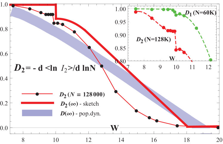
Generalized recursive algorithm for ACAT equations– Following Ref.AbouChacAnd we introduce a single-site Green function, for a site at a generation of the reduced Hamiltonian, obtained from by disconnecting generations and . The random Green functions are characterized by distribution functions, . Individual obey the ACAT recursion equation AbouChacAnd :
| (2) |
where are sites at the generation connected to site . These equations are ill-determined: the pole-like singularities in the right hand sides have to be regularized. This is usually achieved by adding an infinitesimal imaginary part to . The recursion Eq.(2) might become unstable with respect to this addition. This happens for below the critical disorder of the AL transition and manifests the delocalized phase. For the solution is stable. The two types of behavior occur generically in a broad class of Anderson models Anderson .
The spectrum of the Hamiltonian on a finite lattice is given by a discrete set of energies, corresponding to states . Although the global density of states is a sum of delta functions, , it always has a well-defined thermodynamic limit: one introduces an infinitesimal broadening of each delta function, , takes first the limit of the infinite number of sites and afterwards . As a result, tends to a smooth function. In contrast, for the local density of states (LDoS), , the result of this procedure is not always a smooth function. Indeed, in the limit the on-site states are exact eigenstates and even for the infinite system. For finite but large , satellite -like peaks appear. The total number of the peaks is infinite in the thermodynamic limit but almost all of them have exponentially small weight. Hence the effective number of peaks remains finite: it increases as is decreased and becomes infinite at . At this point LDoS becomes smooth provided that the limit is taken before . Note that the opposite order of limits, ( before ) always leads to discrete peaks in LDoS.
At LDoS contains an extensive number of peaks with significant weight: as . Generally, one expects with some . For to be smooth, the broadening should exceed the spacing between the peaks . Thus, the simultaneous limit , , results in a smooth LDoS iff . Studying such generalized limits yields information on the scaling of the number of peaks, i.e. on the structure of the eigenfunctions. Wave functions of ergodic states are uniformly spread on a lattice, so that , i.e. and LDoS is smooth for any . We show below that in a broad interval of disorder strengths in the delocalized regime and equals to the critical value of corresponding to the transition between a smooth and a singular LDoS, .
For (delocalized regime) and an infinitesimal , increases exponentially with the number of recursion steps in Eq.(2) describing an infinite tree:
| (3) |
For a finite RRG of size , radius-graph . For larger the loops terminate the exponential growth of a typical limiting it by . Thus for to be smooth (and independent of ) should scale as , i.e.
| (4) |
Ideally, one would deal with infinitely small in order to determine the exponent . However, the limited precision of any numerical computation makes it impossible in practice: for any realistic initial , the value of becomes significant after few recursions. To avoid this problem we included an additional step to the recursion Eq.(2):
| (5) |
so we keep the typical imaginary part fixed and -independent: (where denotes averaging over all sites in the -th generation). As soon as the stationary distribution of is reached in this recursive procedure, .
To realize this algorithm we adopted a modified population dynamics (PD) method pop-dyn . In each step we used the set of Green functions (”population”) obtained at the previous step and new on-site energies to generate new Green functions according to Eq.(2) in which each site is connected to randomly chosen sites of the previous population set.
In order to obtain one needs to take the limits , of . The convergence turns out to be slow (logarithmic) resulting in a considerable uncertainty in . Luckily, depends only on the combined variable , with , rather than on and separately. Extrapolation of to yields shown in Fig.2.
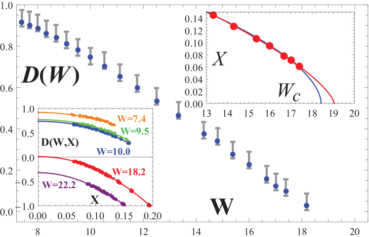
The lower inset of Fig.2 shows the collapse of the data for several and from the intervals and . Since , one needs exceptionally small to reach small . This required computation with higher than usual precision.
Note that the exponent is a property of an infinite BL, . Therefore is free of the finite-size effects which dominate the moments at , where the correlation volume diverges at . The uncertainty of extrapolation of to and turns out to be small enough not to raise doubts that at least in the interval for . Additional support of existence of the phase with comes from the analytical solution to Eq.(2) in the large- limit forthcoming . It turns out that in this limit:
| (6) |
It follows from Eq.(6) that and correspond to the values and of the Lyapunov exponent discussed in Ref.Warzel .
Exact diagonalization on RRG.– While ACAT approach is commonly believed to describe well the localized phase of RRG, its applicability in the delocalized regime requires further inverstigation.
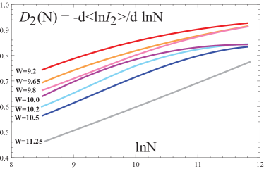
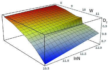
We performed a direct study of the Anderson model on RRG by exact diagonalization at the system sizes up to in the range of disorder strength . The main focus was on calculating the inverse participation ratio and the Shannon entropy for the eigenstates with energies near the band center. The expected asymptotic behavior of the typical averages at is Our-BL :
| (7) |
where are the averages both over the ensemble of RRG with fixed connectivity and over random on-site energies , are the multifractal dimensions and . The derivatives and should saturate at and , respectively in the limit .
We present the results for deep in the delocalized phase (Fig.3) and close to the localization transition (Fig.4).
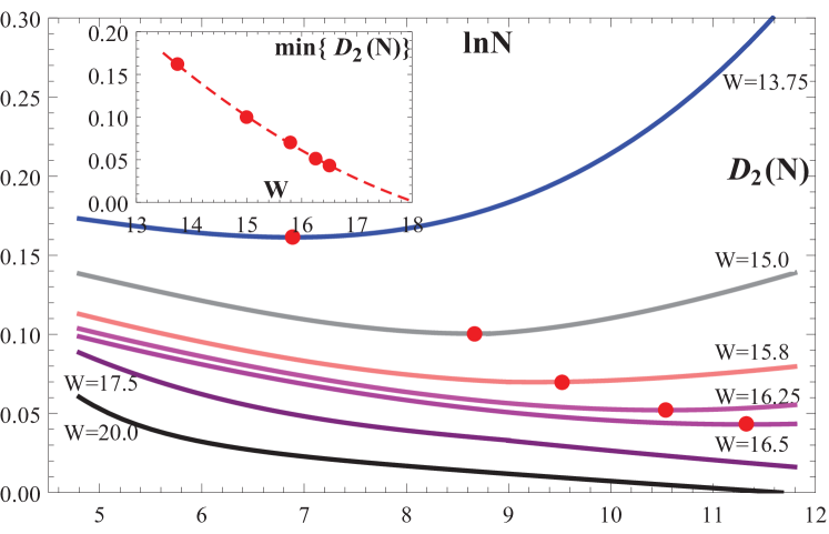
Note two important features on these plots: (i) an abrupt change of behavior for close to and (ii) a minimum in the -dependence of (recently reported in Tikhonov ) in the vicinity of AL transition: as , at the minimum and vanish. Extrapolation of leads to (see inset to Fig.4) in agreement with PD results, Fig.2.
A striking result of the exact diagonalization is the existence of a jump in both and shown in Fig.1. A feature, which is almost invisible at small evolves to a more and more abrupt jump as increases above (see Fig. 3, right panel). Extrapolation of to for gives , whereas . We conclude that on RRG at there is a first order transition from the non-ergodic delocalized phase at to the ergodic one at .
Conclusion.
The existence of the non-ergodic phase of the BL Anderson model together with the similarity of this model with generic many-body
ones gives basis for far-reaching speculations. The point is that in contrast to the conventional Anderson localization, which is
the property of any wave dynamics, the MBL is a genuine quantum phenomenon. Indeed, in the classical limit,
a weakly perturbed integrable system with degrees of freedom always demonstrates some diffusion in the phase space known as
Arnold diffusionArnold . Although the celebrated Kolmogorov Arnold Moser (KAM) theorem KAM
guarantees the survival of the vast majority of the invariant tori the chaotic part of the phase space is
connected (unless ), thus allowing the diffusion for arbitrary weak perturbation.
Therefore one should not expect MBL in the classical limit. On the other hand the glassy
states of matter without doubts exist for any including and are obviously not ergodic. It is safe to assume that the extended non-ergodic phase of the MBL
models is not qualitatively different from a classical glassy state Mezard-glass . Therefore our arguments in
favor of the existence of the delocalized non-ergodic phase of the BL Anderson model and the true phase transition
between the ergodic and non-ergodic states can be considered as arguments in favor of glassy states being distinct
states of matter and their transition to fluids being a true phase transition.
Acknowledgement We appreciate hospitality at KITP of University of California at Santa Barbara under the NSF grant
No.NSF PHY11-25915, at KITPC in Beijing (V. E. K.) and at the Center for Theoretical Physics of Complex Systems (Daejeon, S.Korea) where the research has been carried out. E.C. thanks partial financial support by the Murcia Regional Agency of Science
and Technology (project 19907/GERM/15). The research of L.B.I. was partially supported by the Russian Science
Foundation grant No. 14-42-00044. We are grateful to G. Biroli, E. Bogomolny, J. T. Chalker,
M. V. Feigelman, M. Foster, I. M. Khaymovich, G. Parisi, V. Ros, A. Scardicchio, M. A. Skvortsov, V. N. Smelyanskiy, K. S. Tikhonov and S. Warzel
for stimulating discussions.
References
- (1) D. M. Basko, I. L. Aleiner, and B. L. Altshuler. 321, 1126 (2006).
- (2) P. W. Anderson. Phys. Rev., 109, 1492 (1958).
- (3) V. Oganesyan and D. A. Huse. Phys. Rev. B, 75, 155111 (2007).
- (4) V. Oganesyan, A. Pal, and D. A. Huse. Phys. Rev. B 80 115104 (2009).
- (5) M. Pino, L. B. Ioffe, and B. L. Altshuler. PNAS, 113, 536 (2016).
- (6) B. L. Altshuler, Y. Gefen, A. Kamenev, and L. S. Levitov. Phys. Rev. Lett., 78 2803 (1997).
- (7) R. Abou-Chacra, D.J. Thouless, and P.W. Anderson. J. of Phys. C (Solid State Physics), 6, 1734 (1973).
- (8) M. Aizenman, S. Warzel, J. Eur. Math. Soc. 15, 1167 (2013).
- (9) M. Aizenman and S. Warzel, Europhys. Lett. 96, 37004 (2011).
- (10) G. Biroli, A. Ribeiro-Teixeira, and M. Tarzia, arXiv:1211.7334.
- (11) A. De Luca, B. L. Altshuler, V. E. Kravtsov and A. Scardicchio, Phys. Rev. Lett., 113, 046806 (2014).
- (12) A. D. Mirlin and Y. V. Fyodorov, Phys. Rev. Lett. 72, 526 (1994); A. D. Mirlin and Y. V. Fyodorov, J. Phys. I (France) 4, 655 (1994); Y. V. Fyodorov and A. D. Mirlin, Phys. Rev. Lett. 67, 2049 (1991); A. D. Mirlin and Y. V. Fyodorov, Phys. Rev. B 56, 13393 (1997).
- (13) E. Targuini, G. Biroli, M. Tarzia, Phys. Rev. Lett. 116, 010601 (2016).
- (14) V. E. Kravtsov, I. M. Khaymovich, E. Cuevas, M. Amini, New J. Phys. 17, 122002 (2015).
- (15) F. L. Metz, I. Perez Castillo, Large deviation function for the number of eigenvalues of sparse random graphs inside an interval. arXiv:1603.06003
- (16) K. S. Tikhonov, A. D. Mirlin, and M. A. Skvortsov, Anderson localization on random regular graphs. arXiv:1604.05353 (2016).
- (17) X. Deng, B.L. Altshuler, G.V. Shlyapnikov, L. Santos, Quantum Levy flights and multifractality of dipolar excitations in a random system. arXiv:1604.03820.
- (18) The multifractal statistics was observed also in the numerical study [C. Monthus and T. Garel, J. Phys. A 44, 145001 (2011)] of distribution of conductances between the root and the exturnal leeds conneceted to boundary points of a finite tree.
- (19) B. Bollobas, Random graphs, Second edition, Cambridge studies in advanced Mathematics 73, pp. 264-267, Cambridge University Press, 2001.
- (20) M. M ezard and G. Parisi, Eur. Phys. J. B 20, 217-233 (2001).
- (21) M. M ezard and A. Montanari, Information, physics, and computation, (Oxford University Press, 2009).
- (22) see online Supplementary Material.
- (23) B. L. Altshuler, L. B. Ioffe and V. E. Kravtsov (in preparation).
- (24) V. I. Arnol d, Instability of dynamical systems with several degrees of freedom, (Russian, English) Sov. Math., Dokl., 5, 581 (1964); translation from Dokl. Akad. Nauk SSSR, 156, 9 (1964).
- (25) A. N. Kolmogorov. On conservation of conditionally periodic motions under small perturbations of the hamiltonian. Dokl. Akad. Nauk, SSSR, 98, 527 (1954); V.I. Arnol d, Proof of a theorem by A.N. Kolmogorov on the invariance of quasi-periodic motions under small perturbations of the Hamiltonian, Russian Math. Surveys 18,9 (1963); J. Moser. On invariant curves of area-preserving mappings of an annulus. Nachr. Akad. Wiss., G ottingen, Math. Phys. Kl., pages 1 20, (1962); V. I. Arnold, Mathematical Methods of Classical Mechanics, Springer-Verlag (1989).
- (26) M. Mezard, First steps in glass theory, in: M.P. Ong, R.N. Bhatt (Eds.), More is different, Princeton University Press, Princeton, New Jersey, 2001.
I Supplementary material
I.1 Analysis of statistics of inverse participation ratio for RRG and 3D Anderson model in the delocalized phase.
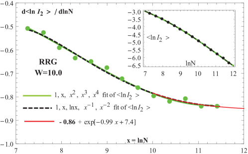
In order to evaluate the fractal dimensions and we performed an exact diagonalization of matrix Hamiltonians drawn from the ensemble of (i) different RRG with branching number and a fixed total number of sites ranging from to and (ii) different realizations ( for the largest and ) of the independent random on-site energies with the box distribution characterized by the disorder strength . For the largest and we analyzed eigenstates with energies close to the band-center.
For each value of this step of the calculation results in a set of -dependent ensemble averages
| (8) |
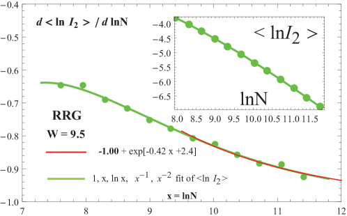
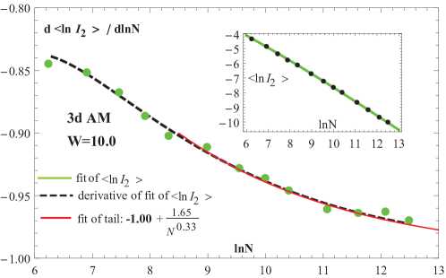
where are the wave function coefficients of a state at a site . The averages are presented by points in the inserts of Fig.5.-Fig.7. We define the running fractal dimensions and as derivatives
| (9) |
respectively, since the limits of these derivatives are by definition and . It is convenient to first find a smooth multi-parameter approximations of the dependencies of and on and then evaluate the derivatives of these smooth interpolating functions. Typical 5-parameter interpolating functions are shown in Fig.5. We also evaluated discrete derivatives (green points in Fig.5-Fig.7).
The last step was to find the best power-law (exponential in ) fit
| (10) |
of the large- tail of the smooth interpolating functions (red solid curves in Fig.5.-Fig.7). Our values of fractal dimensions follow from this extrapolation. The procedure described above yields not distinguishable form 1 for (e.g. for shown in Fig.6 it gives ). At the same time for the best fit results in distinctly different from 1. We checked that the analogous procedure for the three-dimensional Anderson model in the delocalized phase with yields (Fig.7) with all the dependencies similar to the ones for RRG at ( Fig.6). This analysis led us to the conclusion that the finite- jump in shown in Fig.1 of the main paper survives the thermodynamic limit and implies the first order transition to the ergodic phase for .
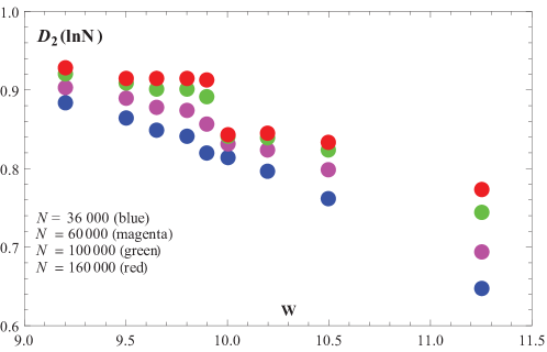
Another evidence of the transition at is the singularity at in the speed of evolution with of . In Fig.8 it is shown that while generally increases with increasing , the speed of this evolution reaches a deep minimum at , making the convergence better at than both for and for .
In Fig.9 we further illustrate this point: the difference shows a sharp singularity at . We would like to emphasize that no extrapolation was employed.
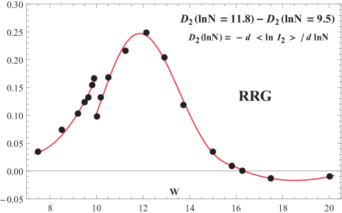
Both features, (i) the jump in , and (ii) the anomaly in the speed of evolution, prove that the phase that exists on RRG for may not be ergodic. We argue that the singularity of function at completely excludes the possibility of the states in the interval being ergodic.