Two-dimensional Infrared Spectroscopy of vibrational polaritons of molecules in an optical cavity.

Abstract

Strong coupling of molecular vibrations to an infrared cavity mode affects their nature by creating dressed polariton states. We show how the single and double vibrational polariton manifolds may be controlled by varying the cavity coupling strength, and probed by a time domain 2DIR technique, Double Quantum Coherence (DQC). Applications are made to the amide-I ($CO$) and amide-II ($CN$) bond vibrations of $N-methylacetamide$ (NMA).

I Introduction

Elementary physical and chemical properties of molecules can be modified by coupling them to the optical modes of a cavity thus forming strongly coupled $matter+field$ states known as polaritons Berman (1994); Haroche and Raimond (2006). These have been widely studied in atoms. Electronic polaritons in molecules have been extensively studied both experimentally and theoretically Coles et al. (2014a, b); Herrera et al. (2014). Vibrational polaritons in the infrared has been recently demonstrated in molecular aggregates Shalabney et al. (2015a); del Pino et al. (2015); Shalabney et al. (2015b); Simpkins et al. (2015) and in semiconductor nano-structures Autry et al. (2015); Sun et al. (2015); Wilmer et al. (2015). The radiation matter coupling is related to cavity frequency $\omega_{c}$ by, $g_{i}=\sqrt{N}\bm{\mu}_{i}\cdot\bm{e}_{c}\sqrt{\left(\hbar\omega_{c}/2\epsilon_{0}V\right)},$ where, $N$ is the number of molecules. $\bm{\mu}_{i}$ is the transition dipole moment of the mode $i$, $\bm{e}_{c}$ is the cavity electric field vector, $\epsilon_{0}$ is vacuum permittivity, and $V$ is the cavity mode volume Savona et al. (1995); Berman (1994); Feist and Garcia-Vidal (2015); Shalabney et al. (2015a); del Pino et al. (2015); Shalabney et al. (2015b); Simpkins et al. (2015). While strong coupling to cavity modes has been realized even for a single atom, $N=1$,Berman (1994); Haroche and Raimond (2006); Faez et al. (2014) polaritons in organic molecules were reported for large $N(\sim 10^{17})$ Shalabney et al. (2015a). With the advent of anomalous refractive index materials Alù et al. (2007); Fleury and Alù (2013), sub-wavelength Fabry-Perot microcavities Kelkar et al. (2015), and nanocavities Benz et al. (2015) it may become possible to achieve strong cavity coupling of single molecules.

Coherent multidimensional infrared spectroscopy is a powerful time domain tool that can probe anharmonicities and vibrational energy relaxation pathways Lai et al. (2013); Abramavicius et al. (2008); Venkatramani and Mukamel (2002); Piryatinski et al. (2001); Greve et al. (2013). Vibrational polaritons were experimentally reported Shalabney et al. (2015a, b); Simpkins et al. (2015) and calculated del Pino et al. (2015); Cwik et al. (2015) recently. Multidimensional spectroscopic studies for electronically excited states in semiconductor cavity for nano-particles like $In_{0.04}Ga_{0.96}As$ has been demonstrated Wilmer et al. (2015); Nardin (2015). Similarly, electronic exciton-polariton interactions of quantum wells in microcavity Takemura et al. (2015) has also been reported. Bipolaritons generated using four wave mixing techniques have been used as efficient entangled photon source Oka and Ishihara (2008a, b).

In this article, we calculate 2DIR signals for vibrational polaritons, focusing specially on the double quantum coherence (DQC) technique. Studying DQC of molecular vibrational polaritons in optical cavity can be used to study the effects of strong couplings on the vibrational anharmonicities and consequently allow us to control these anharmonicities. We introduce DQC signal in next section (Sec.II), we then study single vibrational mode (Amide-I of NMA) coupled to a single mode cavity and calculate DQC in section (Sec.III), followed by two vibrational modes (Amide-I+II of NMA) coupled to a single mode cavity (Sec.IV); and finally conclude in Sec. V.

II Vibrational polaritons and their DQC signal

Vibrational modes (Fig. 1) coupled to an infrared cavity under the Rotating Wave Approximation (RWA) are described by the hamiltonian Chernyak et al. (1998); Abramavicius et al. (2009); Roslyak et al. (2010); Shalabney et al. (2015a); del Pino et al. (2015); Shalabney et al. (2015b); Simpkins et al. (2015),

$$H_{0} = \omega_{c}(\theta)a^{\dagger}a+\sum_{i}^{m}\omega_{i}b_{i}^{\dagger}b_{i}+\sum_{i\neq j}^{m}J_{ij}b_{i}^{\dagger}b_{j}$$ (1)

$$- \sum_{ij}^{m}\frac{\Delta_{ij}}{2}b_{i}^{\dagger}b_{j}^{\dagger}b_{i}b_{j}+\sum_{i,j=1}^{m}g_{i}\left(a^{\dagger}b_{i}+b_{i}^{\dagger}a\right),$$

where, $a(a^{\dagger})$ and $b(b^{\dagger})$ are annihilation(creation) operators for the cavity photon, and vibrational excitation respectively, which satisfy boson commutation relations, $[a,a^{\dagger}]=1;[b_{i},b_{j}^{\dagger}]=\delta_{ij}$ and $\hbar=1$. $\omega_{c}(\theta)=\omega_{0}\left(1-\frac{\sin^{2}(\theta)}{n^{2}_{eff}}\right)^{-1/2}$, is the angle-dependent cavity energy with $\omega_{0}$ being cavity cut-off (or maximum) energy and, $\theta$ the angle of incidence to the cavity mirrors. We set $\theta=0^{\circ}$ for simplicity. $\omega_{i}$ is vibrational frequency of mode $i$. $J_{ij}$ is the scalar coupling between two vibrational modes $i$ and $j$, while $\Delta_{ij}$ is the anharmonicity between respective modes. Finally, the coupling strength of vibrational modes $i$ to an optical mode is, $g_{i}$ as described in introduction.

The cavity volume $(V=(\lambda/n_{eff})^{3})$ depends on cavity resonance wavelength ($\lambda$) and effective intra-cavity refractive index ($n_{eff}$) Savona et al. (1995); Berman (1994); Feist and Garcia-Vidal (2015). Decreasing $n_{eff}$ can also be used for strong coupling to single molecular vibrational excitation, for instance, when the refractive indices of one of the two layers’ of a Distributed Bragg Reflector (DBR) Fabry-Perot is equal to the empty cavity refractive index $n_{c}$, say $n_{c}=(n_{2}\veebar n_{1})$, then $n_{eff}=\sqrt{n_{1}n_{2}}$. In this case, choosing either one of the layers to be material with anomalous refractive index may decrease $n_{eff}<1$ Kelkar et al. (2015). The vacuum Rabi splitting $\Omega_{R}$ of mode $i$ is $2\hbar g_{i}$.

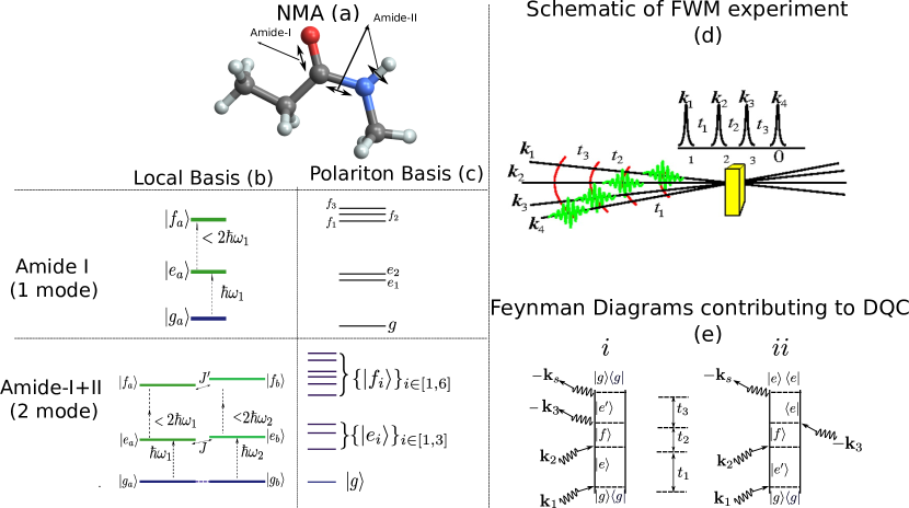
Figure 1: Amide-I ($C=O$ symmetric stretch) and Amide-II ($CN$ symmetric stretch + $NH$ bend) vibrations are represented using double sided arrow for $N-Methylacetamide$ in (a). Eigen-energies of Amide-I and coupled Amide-I and Amide-II motifs in local basis and polariton basis (see Sec.SI of supplementary information supp for detail) are given in (b) and (c) respectively. (d) schemes the FWM experiment, the yellow sample is the DBR Fabry-Perot cavity coupled to molecular vibrations (see text for detail) and, (e) shows the relevant ladder diagrams contributing to double quantum coherence (DQC) technique.

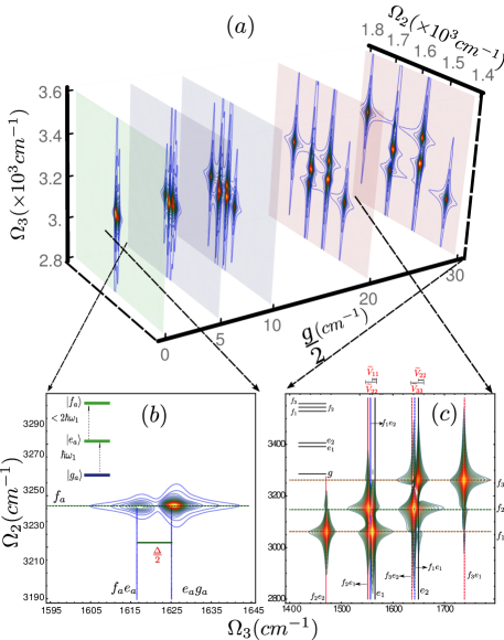
Figure 2: (a) Absolute value of DQC signal (Eq. 3) for Amide-I vibrations of NMA, as we vary coupling strength ($g$) from no (green plane), weak (blue planes) and strong (red planes) coupling regimes. (b) Schematic representation of DQC signal (zoomed in the grey square at $g=0cm^{-1}$) with all possible peaks identified as intersections of different lines. (c) Same result but for strong coupling and the last panel. The lines are: i) $\Omega_{fe}$ labelled as $f_{i}e_{j}$ (dashed blue lines), ii) $\Omega_{eg}$ labelled as $e_{j}$ (black solid lines), iii) $\Omega_{fg}$ labelled as $f_{i}$ and appropriate anharmonicities ($\Delta_{ij}$ in local basis or $\widetilde{V}_{ii}$ in polariton basis) respectively. We wish to spectrally resolve (b) to (c).

DQC is a four wave mixing signal generated by three chronologically ordered pulses with wavevectors $\bm{k}_{1}$, $\bm{k}_{2}$ and $\bm{k}_{3}$ and detected by with a fourth pulse in the direction, $\bm{k_{III}}=\bm{k}_{1}+\bm{k}_{2}-\bm{k}_{3}$ (Fig.1 (e)) (Abramavicius et al., 2008; Mukamel, 1999). The signal is recorded versus three time delays $t_{1}$, $t_{2}$ and $t_{3}$. We assume a three polariton manifold as shown in Fig. 1. Using the ladder diagrams for DQC (Fig. 1e) in polariton basis, which diagonalizes the first three and last terms of Eq. 1 (Fig. 1, Sec.SI of supplementary information supp ), we see that system oscillates with frequency $\Omega_{eg}=\Omega_{e}-\Omega_{g}$ during time delay $t_{1}=\tau_{2}-\tau_{1}$ and with frequency $\Omega_{fe}=\Omega_{f}-\Omega_{e}$ during delay $t_{2}=\tau_{3}-\tau_{2}$ in both contributing diagrams (Fig. 1e). After the third pulse the system oscillates either with frequency $\Omega_{e^{\prime}g}$ or $\Omega_{e^{\prime}f}$ during the delay $t_{3}=\tau_{4}-\tau_{3}$. For harmonic case, $\Omega_{e^{\prime}g}=\Omega_{e^{\prime}f}$ where the DQC signal vanishes. A 3D signal $\mathcal{S}(t_{3},t_{2},t_{1})$, which can be written as double Fouier transform with respect to $t_{2}$ and $t_{3}$ as (Abramavicius et al., 2008),

$$\mathcal{S}(\Omega_{3},\Omega_{2},t_{1})=\int\int_{0}^{\infty}dt_{3}dt_{2}e^{i(\Omega_{3}t_{3}+\Omega_{2}t_{2})}\mathcal{S}(t_{3},t_{2},t_{1}).$$ (2)

Upon expanding in polariton eigenstates, the signal with time delay $t_{1}=0$ becomes,

$$\mathcal{S}(\Omega_{3},\Omega_{2},t_{1}=0) = \sum_{ee^{\prime},f}\frac{1}{(\Omega_{2}-\Omega_{fg}+i\gamma_{fg})}$$ (3)

$$\bigg{[}\mu_{e^{\prime}f}\mu_{ge^{\prime}}\mu_{fg}\mu_{ge}\frac{1}{\Omega_{3}-\Omega_{e^{\prime}g}+i\gamma_{e^{\prime}g}}$$

$$- \mu_{ge^{\prime}}\mu_{e^{\prime}f}\mu_{fg}\mu_{eg}\frac{1}{\Omega_{3}-\Omega_{fe}+i\gamma_{fe}}\bigg{]}.$$

Where, $\mu_{ij}$ is the polariton transition dipole from states in manifold $j\to i$ while $\gamma_{ij}$ is the respective dephasing. Note that the polariton eigenstates depend on the effective cavity coupling strengths, $\widetilde{g}_{i}\left(=\sqrt{Ng^{2}_{i}-\frac{1}{4}(\kappa-\gamma_{i})^{2}}\right)$, where $\kappa$ is cavity decay rate, and $\gamma_{i}$ is dephasing rate of respective mode Savona et al. (1995). Tuning the cavity coupling allows to control spectral structures of the singly and doubly excited vibrational polariton manifolds (Fig.2 and can be captured using DQC as illustrated in the following section (Sec. III).

III A Single vibrational mode coupled to single cavity mode

The Amide motifs ($O=C-N-H$) link the amino-acid in peptides containing fundamental structural information, for instance, backbone geometry, interactions with hydrogen bonds and dipole-dipole interactions Hayashi and Mukamel (2008). 2D spectroscopy of the amide-I and II symmetric vibrations ( Fig. 1e ) have been studied Rubtsov et al. (2003); Lai et al. (2013). We focus on the Amide-I vibrations in NMA (Table. 1). We consider a single Amide-I stretch mode in resonance with the cavity mode and large anharmonicity $(\Delta_{ij}>\gamma_{ij}$) with varying coupling strengths $\widetilde{g}_{1}$ ranging from $0$ to $80$ $cm^{-1}$ (Table. 1). For a single vibrational mode (Fig.1), the three polariton manifolds have a ground state ($g$), two single excited states ($e$) and three doubly excited states ($f$). Furthermore, for detuning ($\delta=\omega_{1}-\omega_{c}$), the polariton basis modifies the anharmonicity $\Delta_{11}(\to\widetilde{V}_{11}=16\Delta_{11}|\widetilde{g}_{1}^{4}/(\delta^{2}-16\widetilde{g}_{1}^{2})^{2}|)$.

Table 1: Parameters used in this work. $\omega_{0}$ is cavity cut-off frequency. $\omega_{1,2}$ are vibrational exciton (1,2) ($Amide-I,Amide-II$) energies (Barth, 2007; DeFlores et al., 2006), $\gamma_{1,2}$ are their respective dephasing rates, $J_{ij}$ is harmonic scalar coupling, and $\Delta_{ij}$ are exciton-exciton interaction energies.

(in $cm^{-1}$ )	Cavity	Amide-I	Amide-I+II
Energy	$\omega_{0}$=1625	$\omega_{1}$=1625	$\omega_{1}$=1625, $\omega_{2}$=1545
Dephasing	$\kappa$=0	$\gamma_{1}$=20	$\gamma_{1}=\gamma_{2}$=20
Anharmonicities (Local basis)	$\Delta_{00}=0$	$\Delta_{11}$=15	$\Delta_{11}$=15,$\Delta_{22}$=11 $\Delta_{21}=\Delta_{12}$=10
Scalar coupling	-	-	$J_{12}$=15
Eff. refractive ind.	$n_{eff}$ =0.5	-	-
Anharmonicities (Polariton basis)	$\widetilde{V}_{ij}=\frac{\Delta_{ij}}{2}|X_{i}|^{2}|X_{j}|^{2}$

Using Eq. 3 and ladder diagrams (Fig. 1e) the signals $|\mathcal{S}_{i}(\Omega_{3},\Omega_{2},0)|$, $|\mathcal{S}_{ii}(\Omega_{3},\Omega_{2},0)|$ and $|\mathcal{S}(\Omega_{3},\Omega_{2},0)=|\mathcal{S}_{i}(\Omega_{3},\Omega_{2},0)+\mathcal{S}_{ii}(\Omega_{3},\Omega_{2},0)|$ are shown in Fig. 3 and 4 in left, center and right columns respectively (sec. III). Absolute values are shown to illustrate peak assignments and affects of varying coupling strengths ($\widetilde{g}_{i}$). For completness, the respective absorptive (Im) and dispersive (Re) parts of the DQC signals are shown in Sec.SIIIA in supp . The peak splittings depends on coupling strengths ($\widetilde{g}_{i}$) and polariton anharmonicities ($\widetilde{V}_{ij}$) and are given Sec.SV of  supp .

Free molecule (Fig. 3): The Amide-I vibrations in NMA (without cavity) is a simple three level system as shown in Fig. 1. Under this condition, $e_{1}=e_{2}$ and $f_{1}=f_{2}=f_{3}$, thus we only observe single peak resonant at $\Omega_{fg}=3168cm^{-1}$ on $\Omega_{2}$ axis. The peaks due to $|\mathcal{S}_{i}(\Omega_{3},\Omega_{2},0)|$ (Fig. 3(a)) shows $\Omega_{eg}=1625cm^{-1}$ resonance, while $|\mathcal{S}_{ii}(\Omega_{3},\Omega_{2},0)|$ (Fig. 3(b)) shows resonance at $\Omega_{fe}=1617cm^{-1}$ along $\Omega_{3}$ axis. The total signal (Fig. 3(c)) thus shows two peaks due to resonances at $\Omega_{eg}$ and $\Omega_{fe}$.

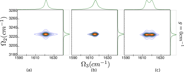
Figure 3: DQC signals for Amide-I vibrations in NMA using Eq. 3 and ladder diagrams (Fig. 1e): (a) $|\mathcal{S}_{i}(\Omega_{3},\Omega_{2},0)|$ with resonance at $\Omega_{eg}=1625cm^{-1}$, (b)$|\mathcal{S}_{ii}(\Omega_{3},\Omega_{2},0)|$ with resonance at $\Omega_{fe}=1617cm^{-1}$ and (c)$|\mathcal{S}(\Omega_{3},\Omega_{2},0)|$ with resonances at $\Omega_{eg}=1625cm^{-1}$ and $\Omega_{fe}=1617cm^{-1}$. The linear projections along each axis is shown in green. For simplicity, cavity field vector $\bm{e}_{c}$ is assumed to be mostly parallel to molecular vibrational transition dipole $\mu_{m}$. Amide-I vibrations ($\omega_{1}$) is resonant to cavity cutoff frequency $\omega_{0}=1625cm^{-1}$. The anharmonicity are assumed $\Delta_{11}=15cm^{-1}$ (Table  1).

Weak coupling regime (Fig. 4-top row) with $\widetilde{g}$=$20cm^{-1}$: Upon varying the coupling strength, there are two singly excited and three doubly excited polariton states (Fig.  1 b-c, Sec SII-S1 of supp ). We thus observe that all $|\mathcal{S}_{i}(\Omega_{3},\Omega_{2},0)|$, $|\mathcal{S}_{ii}(\Omega_{3},\Omega_{2},0)|$ and $|\mathcal{S}(\Omega_{3},\Omega_{2},0)|$ show three distinct peaks along $\Omega_{2}$ axis with energies resonant to $\Omega_{f_{1}g}=2\Omega_{e_{1}g}-\widetilde{V}_{11}$, $\Omega_{f_{2}g}=2\Omega_{e_{1}g}$ and $\Omega_{f_{3}g}=2\Omega_{e_{2}g}-\widetilde{V}_{33}$ respectively. Along $\Omega_{3}$ axis, $|\mathcal{S}_{i}(\Omega_{3},\Omega_{2},0)|$ (Fig. 4(top,left)) shows peak resonance at $\Omega_{e_{1}g}$ and $\Omega_{e_{2}g}$ with splitting $\sim\widetilde{g}$. The $|\mathcal{S}_{ii}(\Omega_{3},\Omega_{2},0)|$ (Fig. 4(top, middle)) has six distinct peaks at energies resonant to $\Omega_{f_{2},e_{2}}$, $\Omega_{f_{2},e_{1}}$, $\Omega_{f_{1},e_{2}}$, $\Omega_{f_{3},e_{2}}$, $\Omega_{f_{1},e_{1}}$, $\Omega_{f_{3},e_{1}}$ in increasing order respectively. The $|\mathcal{S}(\Omega_{3},\Omega_{2},0)|$ (Fig. 4(top, right)) has diminished peaks at $\Omega_{f_{2}e_{1}}$ and $\Omega_{f_{3}e_{2}}$ due to destructive interference of $\Omega_{f_{2}e_{1}}$ with $\Omega_{e_{1}g}$ and $\Omega_{f_{3}e_{2}}$ with $\Omega_{e_{2}g}$ resonances.

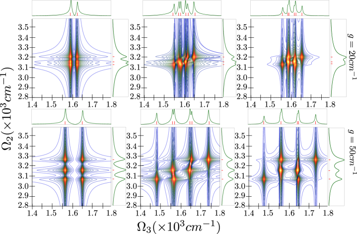
Figure 4: DQC signals using Eq. 3 and ladder diagrams (Fig. 2b): $Columns$ $(\text{left}-)|\mathcal{S}_{i}(\Omega_{3},\Omega_{2},0)|$ with resonance at $\Omega_{e_{1}g}$ and $\Omega_{e_{2}g}$; $(\text{middle}-)|\mathcal{S}_{ii}(\Omega_{3},\Omega_{2},0)|$ with resonance at $\Omega_{f_{2},e_{2}}$, $\Omega_{f_{2},e_{1}}$, $\Omega_{f_{1},e_{2}}$, $\Omega_{f_{3},e_{2}}$, $\Omega_{f_{1},e_{1}}$, $\Omega_{f_{3},e_{1}}$ ; and $(\text{right}-)|\mathcal{S}(\Omega_{3},\Omega_{2},0)|$ with respective resonances for Amide-I vibrations in NMA with cavity coupling $rows:$ $(a)20cm^{-1}$ and $(a)50cm^{-1}$. The linear projections along each axis is shown in green. For simplicity, cavity field vector $\bm{e}_{c}$ is assumed to be mostly parallel to molecular vibrational transition dipole $\mu_{m}$. Amide-I vibrations ($\omega_{1}$) is resonant to cavity cutoff frequency $\omega_{0}=1625cm^{-1}$. The anharmonicity are assumed $\Delta_{11}=15cm^{-1}$ (Table  1)

Strong coupling regime (Fig. 4-bottom row) with $\widetilde{g}=50cm^{-1}$: The signals corresponding to $|\mathcal{S}_{i}(\Omega_{3},\Omega_{2},0)|$ (Fig. 4(bottom, left)), $|\mathcal{S}_{ii}(\Omega_{3},\Omega_{2},0)|$ (Fig. 4(bottom, middle)) and $|\mathcal{S}(\Omega_{3},\Omega_{2},0)|$ (Fig. 4(bottom, right)) show peaks corresponding to $\Omega_{f_{1}g}$, $\Omega_{f_{2}g}$ and $\Omega_{f_{3}g}$ along $\Omega_{2}$ axis. Projections on $\Omega_{3}$ axis for $|\mathcal{S}_{ii}(\Omega_{3},\Omega_{2},0)|$ six peaks assigned as in weak coupling case, however the peak splitting between resonance pairs with energies $(\Omega_{f_{2}e_{1}},\Omega_{f_{1}e_{2}})$ and $(\Omega_{f_{3}e_{2}},\Omega_{f_{1}e_{1}})$ remains relatively constant and proportional to respective contributing anharmonicities. The total signal shows six peaks due to $\Omega_{f_{2}e_{1}}$ and $\Omega_{f_{3}e_{2}}$ diminished because of destructive interferences from resonances of singly excited polaritons.

This partial cancellation of peaks puts an upper bound on strong coupling strengths for fully resolved DQC signals. Furthermore by changing $t_{1}$, we can observe the dynamics in singly and doubly excited polariton manifolds to obtain bountiful information regarding lifetimes of molecular vibrational bipolaritons. In case of zero detuning ($\delta=\omega_{1}-\omega_{c}=0$), the doublet peak splitting due to $\widetilde{V}_{11}$ is independent of coupling strength $i.e.,\widetilde{V}_{11}=\Delta/32$. Thus DQC can be used as direct measurements of anharmoncities due to vibrational polariton-polariton interactions for vanishing detuning cases. One has to be careful however, for $\delta\neq 0$ cases; as such conditions allow the anharmonicities to vary non-trivially ($\sim 16\Delta_{11}|\widetilde{g}_{1}^{4}/(\delta^{2}-16\widetilde{g}_{1}^{2})^{2}|$). This may cause destructive interference of different peaks along $\Omega_{3}$ axis.

IV Polaritons for two vibrational modes and their DQC signal

We now couple the Amide-I and Amide-II vibrations (Fig. 1, Rubtsov et al. (2003)) of a single NMA molecule ($N=1$) to an infrared cavity. We next calculate the double quantum coherence (DQC) signals for vibrational molecular polaritons (Fig. 1 (e), Eq. 3) utilizing Eqs.S2-S5 (of supplementary material supp ).

The overlapping of peaks due to anharmonicities is better illustrated in case of Amide-I+II vibrations coupled to single mode cavity. We next present three coupling regimes for such a condition. We assume $\widetilde{g}_{1}/\widetilde{g}_{2}=constant$ for simplicity. The remainder of relevant parameters are shown in Table  1.

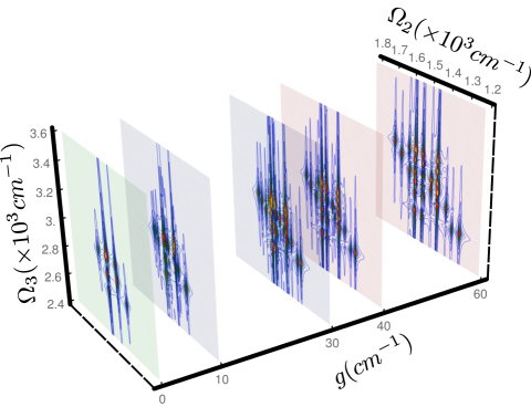
Figure 5: Modulus of DQC signal for Amide-I+II vibrations in NMA with varying cavity coupling ($0cm^{-1}\to 60cm^{-1}$). Cavity field vector $\bm{e}_{c}$ is assumed to be mostly parallel to molecular vibrational transition dipole $\mu_{m}$. Amide-I vibrations ($\omega_{1}$) is resonant to cavity cutoff frequency $\omega_{0}=1625cm^{-1}$ and $\omega_{2}=1540cm^{-1}$. The anharmonicies $\Delta_{11}=15cm^{-1}$ and $\Delta_{22}=11cm^{-1}$ (Table  1).

No cavity (Fig. 6)(a): The coupled Amide-I+II vibrations of NMA is effectively a three level system with two singly excited states and three doubly excited states in absence of cavity coupling. The two singly excited states are resonant with $\Omega_{e_{1}g}$ and $\Omega{e_{2}g}$. The three doubly excited states are resonant with frequencies $\Omega_{f_{1}g}=2\Omega_{e_{1}g}-\Delta_{11}$, $\Omega_{f_{2}g}=\Omega_{e_{1}g}+\Omega_{e_{2}g}$ and $\Omega_{f_{3}g}=2\Omega_{e_{2}g}-\Delta_{22}$ (Sec. SII of supplementary material  supp , Table 1). These peaks are observed along $\Omega_{2}$ axis. Whereas, we only observe four peaks along $\Omega_{3}$ axis in (Fig. 6(a, right column)) because the tuples $(\Omega_{f_{2}e_{1}},\Omega_{f_{1}e_{2}}),\Omega_{e_{1}g})$ and $(\Omega_{f_{3}e_{2}},\Omega_{f_{1}e_{1}}),\Omega_{e_{2}g})$ cannot be resolved due to anharmonicities ($\Delta_{ii}$, Table  1).

Weak coupling regime with $\widetilde{g}=10cm^{-1}$ (Fig. 6)(b): Under these conditions, we observe five peaks along $\Omega_{2}$ axis corresponding to $\Omega_{f_{1}g}$,$\Omega_{f_{2}g}$,$\Omega_{f_{3}g}$,$\Omega_{f_{4}g}$,$\Omega_{f_{5}g}=\Omega_{f_{6}g}$. Projections along $\Omega_{3}$ axis shows two peaks for $|\mathcal{S}_{i}(\Omega_{3},\Omega_{2},0)|$ (Fig. 6(b,bleft column)) resonant with frequencies $\Omega_{e_{1}g}$, $\Omega_{e_{2}g}\approx\Omega_{e_{3}g}$. For $|\mathcal{S}_{ii}(\Omega_{3},\Omega_{2},0)|$ (Fig. 6(b,bmiddle column)) we would ideally expect eighteen peaks corresponding to $\Omega_{f_{1}e_{3}}$, $\Omega_{f_{1}e_{2}}$, $\Omega_{f_{3}e_{4}}$, $\Omega_{f_{4}e_{2}}$, $\Omega_{f_{2}e_{3}}$, $\Omega_{f_{2}e_{2}}$, $\Omega_{f_{1}e_{1}}$, $\Omega_{f_{3}e_{3}}$, $\Omega_{f_{3}e_{2}}=\Omega_{f_{4}e_{1}}=\Omega_{f_{6}e_{3}}$, $\Omega_{f_{6}e_{2}}$, $\Omega_{f_{5}e_{3}}$, $\Omega_{f_{2}e_{1}}$, $\Omega_{f_{5}e_{2}}$, $\Omega_{f_{3}e_{1}}$, $\Omega_{f_{6}e_{1}}$, $\Omega_{f_{5}e_{1}}$ in energetically increasing order. However, only twelve peaks are observed due to overlapping caused by anharmonicities and coupling strength. Similar to Amide-I vibrations of NMA in cavity, we observe fewer peaks in $|\mathcal{S}(\Omega_{3},\Omega_{2},0)|$ (Fig. 6(b, right column)) than that of $|\mathcal{S}_{ii}(\Omega_{3},\Omega_{2},0)|$ due to destructive interferences between $|\mathcal{S}_{ii}(\Omega_{3},\Omega_{2},0)|$ and $|\mathcal{S}_{i}(\Omega_{3},\Omega_{2},0)|$.

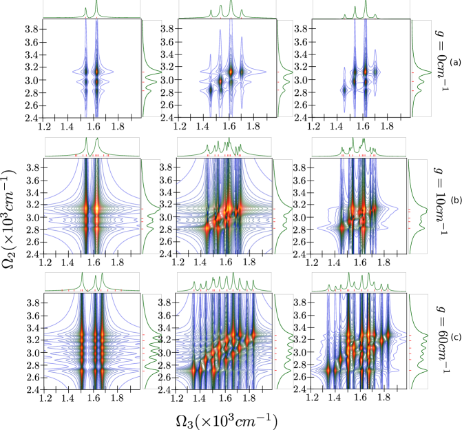
Figure 6: DQC signals for Amide-I+II vibrations in NMA using Eq. 3 and ladder diagrams (Fig. 1e): $Columns:$ $(\text{left-})|\mathcal{S}_{i}(\Omega_{3},\Omega_{2},0)|$ with resonance at $\Omega_{e_{1}g}$, $\Omega_{e_{2}g}$ and $\Omega_{e_{3}g}$ ; $(\text{middle-})|\mathcal{S}_{ii}(\Omega_{3},\Omega_{2},0)|$ with resonance at $\Omega_{f_{1}e_{3}}\approx\Omega_{f_{1}e_{2}}$, $\Omega_{f_{3}e_{4}}\approx\Omega_{f_{4}e_{2}}$, $\Omega_{f_{2}e_{3}}\approx\Omega_{f_{2}e_{2}}$, $\Omega_{f_{1}e_{1}}$, $\Omega_{f_{3}e_{3}}\approx\Omega_{f_{3}e_{2}}=\Omega_{f_{4}e_{1}}=\Omega_{f_{6}e_{3}}$, $\Omega_{f_{6}e_{2}}$, $\Omega_{f_{5}e_{3}}$, $\Omega_{f_{2}e_{1}}$, $\Omega_{f_{5}e_{2}}$, $\Omega_{f_{3}e_{1}}$, $\Omega_{f_{6}e_{1}}$, $\Omega_{f_{5}e_{1}}$ and $(\text{right-})|\mathcal{S}(\Omega_{3},\Omega_{2},0)|$ with respective resonances and cavity couplings ($rows$) (a)$0cm^{-1}$, (b)$10cm^{-1}$, and (c) $60cm^{-1}$ along $\Omega_{3}$, while peaks at $\Omega_{f_{1}g}$,$\Omega_{f_{2}g}$,$\Omega_{f_{3}g}$,$\Omega_{f_{4}g}$,$\Omega_{f_{5}g}$ and $\Omega_{f_{6}g}$ along $\Omega_{2}$. The linear projections along each axis is shown in green. For simplicity, cavity field vector $\bm{e}_{c}$ is assumed to be mostly parallel to molecular vibrational transition dipole $\mu_{m}$. Amide-I vibrations ($\omega_{1}$) is resonant to cavity cutoff frequency $\omega_{0}=1625cm^{-1}$ and $\omega_{2}=1540cm^{-1}$. The anharmonicities are assumed $\Delta_{11}=15cm^{-1}$ and $\Delta_{22}=11cm^{-1}$ (Table  1)

Strong coupling regime $\widetilde{g}=50cm^{-1}$ (Fig. 6(c)): Increasing coupling resolves the six bipolariton resonances along $\Omega_{2}$ for all contributions to the DQC signal (Fig. 6(c)). Along $\Omega_{3}$ axis, however, only $|\mathcal{S}_{i}(\Omega_{3},\Omega_{2},0)|$ is more resolved with three peaks corresponding to $\Omega_{e_{1}g}$, $\Omega_{e_{2}g}$ and $\Omega_{e_{3}g}$ with splitting $\sim\widetilde{g}_{i}$. Despite better peak resolution due to coupling strength dependent peak separations, resonances due to overlapping peaks cannot be fully resolved. The total signal (Fig. 6(right column)) only has 10 distinct peaks as a result of destructive interference of energies of $\Omega_{e_{2}g}$ and $\Omega_{e_{3}g}$ with some of the resonances from $|\mathcal{S}_{ii}(\Omega_{3},\Omega_{2},0)|$.

Increasing coupling strengths provides us well resolved molecular vibrational bipolariton manifold structure (along $\Omega_{2}$ axis), however, it may not provide well resolved DQC signals along $\Omega_{3}$ axis requiring a careful tuning of $\widetilde{g}_{i}$.

V Conclusions

The Multidimensional DQC signals shown in Figs. 2 - 6 demonstrate how the ground state vibrational excitation manifolds are modified upon coupling to the cavity modes. The anharmonicities in the case of Amide-I of NMA coupled to cavity (for non-zero detuning $\delta\neq 0$) are modified with cavity coupling strength, $\Delta_{ij}\rightarrow\widetilde{V}_{ij}=16\Delta_{11}|\widetilde{g}_{1}^{4}/(\delta^{2}-16\widetilde{g}_{1}^{2})^{2}|$ and this can be observed in the peak splitting. For zero detuning, the anharmonicitiy is independent of coupling strength, i.e., $\lim_{\delta\to 0}{\widetilde{V}_{ij}}=\Delta_{11}/32$. However, in the case of Amide-I+II of NMA coupled to the infrared cavity anharmonicities in polariton basis varying nontrivially by, $\widetilde{V}_{ij}=1/2\Delta_{ij}|X_{i}|^{2}|X_{j}|^{2}$ where, $X_{i/j}$ depend on higher order of coupling strengths. This causes several peaks to overlap beyond certain cavity coupling and this is why not all expected peaks for $\Omega_{fe}$ can be spectrally resolved in Fig. 6. However, we can use cavity coupling dependent anharmonicities for modifications of ground vibrational structures to mimic weakly interacting molecular vibrational multi-modes.

Controlling and manipulating lifetime of single molecular vibrations by tuning the coupling strengths and time delays between ultrafast pulses (say, $t_{1}$) can reveal new energy transfer mechanisms. Varying cavity polarization ($\bm{\mu}_{k}\cdot\bm{e}_{c}$) and incident angle ($\theta$) in Eq. 1 using collinear experiments Nardin (2015) could provide information regarding spatial confinements of several vibrational excitations and possibilities of molecular vibrational condensates like usual electronic polariton condensates in organic Deng et al. (2010); Bittner et al. (2012); Zaster et al. (2010) and inorganic Deng et al. (2010); Kasprzak et al. (2006); Plumhof et al. (2014) microcavities, if effective dense vibrational polaritons are obtained, which may be possible in larger macromolecules like J-aggregates. Time-varying cavity coupling strengths can be used to study dynamics of efficient cooling of molecular vibrational states for $n-polariton$ manifolds using higher dimensional spectroscopic techniques.

This work can be extended to control collective molecular vibrational excitations, which may be a useful tool in molecular cooling Kowalewski et al. (2011) allowing to perform ultracold experiments even at room-temperature. Furthermore, by varying the time delays one could be able to modify molecular vibrations via cavity and catch them in action in real time. We show that, by varying the cavity coupling strength $(\widetilde{g})$, it is possible to retrieve spectrally well-resolved molecular vibrational polariton(bipolariton) resonances which are otherwise difficult to resolve (see Fig. 2 - 6 for example). Similar results with respect of the anharmonicities and peak redistributions due to cavity coupling can be achieved using other 2DIR techniques, e.g. $\bm{k_{s}}=-\bm{k}_{1}+\bm{k}_{2}+\bm{k}_{3}$ or $\bm{k_{s}}=\bm{k}_{1}-\bm{k}_{2}+\bm{k}_{3}$, however, the full power of DQC measurements presented here for single molecule in optical cavity can be seen more easily for macromolecules. For such larger systems, a different and much faster numerical algorithms utilizing techniques similar to Nonlinear Exciton Equations (NEE) (Abramavicius et al., 2009) will be useful. Studying the dynamics of modified electronic ground states by applying methods developed in Ref. (Mukamel, 1999) can also be done. In addition, incorporating electronic states can similarly be achieved to modify vibrational excitations of electronically excited states.