On Cross-Validated Lasso in High Dimensions

Abstract

In this paper, we derive non-asymptotic error bounds for the Lasso estimator when the penalty parameter for the estimator is chosen using $K$-fold cross-validation. Our bounds imply that the cross-validated Lasso estimator has nearly optimal rates of convergence in the prediction, $L^{2}$, and $L^{1}$ norms. For example, we show that in the model with the Gaussian noise and under fairly general assumptions on the candidate set of values of the penalty parameter, the estimation error of the cross-validated Lasso estimator converges to zero in the prediction norm with the $\sqrt{s\log p/n}\times\sqrt{\log(pn)}$ rate, where $n$ is the sample size of available data, $p$ is the number of covariates, and $s$ is the number of non-zero coefficients in the model. Thus, the cross-validated Lasso estimator achieves the fastest possible rate of convergence in the prediction norm up to a small logarithmic factor $\sqrt{\log(pn)}$, and similar conclusions apply for the convergence rate both in $L^{2}$ and in $L^{1}$ norms. Importantly, our results cover the case when $p$ is (potentially much) larger than $n$ and also allow for the case of non-Gaussian noise. Our paper therefore serves as a justification for the widely spread practice of using cross-validation as a method to choose the penalty parameter for the Lasso estimator.

T1Date: May, 2016. Revised . We thank Mehmet Caner, Matias Cattaneo, Yanqin Fan, Sara van de Geer, Jerry Hausman, James Heckman, Roger Koenker, Andzhey Koziuk, Miles Lopes, Jinchi Lv, Rosa Matzkin, Anna Mikusheva, Whitney Newey, Jesper Sorensen, Vladimir Spokoiny, Larry Wasserman, and seminar participants in many places for helpful comments. Chetverikov’s work was partially funded by NSF Grant SES - 1628889. Liao’s work was partially funded by NSF Grant SES - 1628889.

1 Introduction

Since its invention by Tibshirani in [41], the Lasso estimator has become increasingly important in many fields, and a large number of papers have studied its properties. Many of these papers have been concerned with the choice of the penalty parameter $\lambda$ required for the implementation of the Lasso estimator. As a result, several methods to choose $\lambda$ have been proposed and theoretically justified; see [49], [13], [9], [38], and [4] among other papers. Nonetheless, in practice researchers often rely upon cross-validation to choose $\lambda$, see [19], and in fact, based on simulation evidence, using cross-validation to choose $\lambda$ remains a leading recommendation in the theoretical literature (see textbook-level discussions in [15], [26], and [25]). However, to the best of our knowledge, there exist very few results about properties of the Lasso estimator when $\lambda$ is chosen using cross-validation; see a review below. The purpose of this paper is to fill this gap and to derive non-asymptotic error bounds for the cross-validated Lasso estimator in different norms.

We consider the regression model

$$Y=X^{\prime}\beta+\varepsilon,\quad{\mathrm{E}}[\varepsilon\mid X]=0,$$ (1)

where $Y$ is a dependent variable, $X=(X_{1},\dots,X_{p})^{\prime}$ a $p$-vector of covariates, $\varepsilon$ unobserved scalar noise, and $\beta=(\beta_{1},\dots,\beta_{p})^{\prime}$ a $p$-vector of coefficients. Assuming that a random sample of size $n$, $(X_{i},Y_{i})_{i=1}^{n}$, from the distribution of the pair $(X,Y)$ is available, we are interested in estimating the vector of coefficients $\beta$. We consider triangular array asymptotics, so that the distribution of the pair $(X,Y)$, and in particular the dimension $p$ of the vector $X$, is allowed to depend on $n$ and can be larger or even much larger than $n$. For simplicity of notation, however, we keep this dependence implicit.

We impose a standard assumption that the vector of coefficients $\beta$ is sparse in the sense that $s=s_{n}=\|\beta\|_{0}=\sum_{j=1}^{p}1\{\beta_{j}\neq 0\}$ is relatively small. Under this assumption, the effective way to estimate $\beta$ was proposed by Tibshirani in [41], who introduced the Lasso estimator,

$$\widehat{\beta}(\lambda)=\operatorname*{arg\,min}_{b\in\mathbb{R}^{p}}\left(\frac{1}{n}\sum_{i=1}^{n}(Y_{i}-X_{i}^{\prime}b)^{2}+\lambda\|b\|_{1}\right),$$ (2)

where for $b=(b_{1},\dots,b_{p})^{\prime}\in\mathbb{R}^{p}$, $\|b\|_{1}=\sum_{j=1}^{p}|b_{j}|$ denotes the $L^{1}$ norm of $b$, and $\lambda$ is some penalty parameter (the estimator suggested in Tibshirani’s paper takes a slightly different form but over time the version (2) has become more popular, probably for computational reasons). In principle, the optimization problem in (2) may have multiple solutions, but to simplify presentation and to avoid unnecessary technicalities, we assume throughout the paper, without further notice, that the distribution of $X$ is absolutely continuous with respect to Lebesgue measure on $\mathbb{R}^{p}$, in which case the optimization problem in (2) has the unique solution with probability one; see Lemma 4 in [43]. Without this assumption, our results would apply to the sparsest solution.

To perform the Lasso estimator $\widehat{\beta}(\lambda)$, one has to choose the penalty parameter $\lambda$. If $\lambda$ is chosen appropriately, the Lasso estimator attains the optimal rate of convergence under fairly general conditions; see, for example, [13], [8], and [34]. On the other hand, if $\lambda$ is not chosen appropriately, the Lasso estimator may not be consistent or may have a slower rate of convergence; see [17]. Therefore, it is important to choose $\lambda$ appropriately. In this paper, we show that $K$-fold cross-validation indeed provides an appropriate way to choose $\lambda$. More specifically, we derive non-asymptotic error bounds for the Lasso estimator $\widehat{\beta}(\lambda)$ with $\lambda=\widehat{\lambda}$ being chosen by $K$-fold cross-validation in the prediction, $L^{2}$, and $L^{1}$ norms. Our bounds reveal that the cross-validated Lasso estimator attains the optimal rate of convergence up to certain logarithmic factors in all of these norms. For example, when the conditional distribution of the noise $\varepsilon$ given $X$ is Gaussian, the $L^{2}$ norm bound in Theorem 4.3 implies that

$$\|\widehat{\beta}(\widehat{\lambda})-\beta\|_{2}=O_{P}\left(\sqrt{\frac{s\log p}{n}}\times\sqrt{\log(pn)}\right),$$

where for $b=(b_{1},\dots,b_{p})^{\prime}\in\mathbb{R}^{p}$, $\|b\|_{2}=(\sum_{j=1}^{p}b_{j}^{2})^{1/2}$ denotes the $L^{2}$ norm of $b$. Here, $\sqrt{s\log p/n}$ represents the optimal rate of convergence, and the cross-validated Lasso estimator attains this rate up to a small $\sqrt{\log(pn)}$ factor. Throughout the paper, we assume that $K$ is fixed, i.e., independent of $n$. Our results therefore do not cover leave-one-out cross-validation.

Given that cross-validation is often used to choose the penalty parameter $\lambda$ and given how popular the Lasso estimator is, understanding the rate of convergence of the cross-validated Lasso estimator seems to be an important research question. Yet, to the best of our knowledge, the only results in the literature about the cross-validated Lasso estimator are due to Homrighausen and McDonald [27, 28, 29] and Miolane and Montanari [32] but all these papers imposed extremely strong conditions and made substantial use of these conditions meaning that it is not clear how to relax them. In particular, [28] assumed that $p$ is much smaller than $n$, and only showed consistency of the (leave-one-out) cross-validated Lasso estimator. [29], which strictly improves upon [27], assumed that the smallest value of $\lambda$ in the candidate set, over which cross-validation search is performed, is so large that all considered Lasso estimators are guaranteed to be sparse, but, as we explain below, it is exactly the low values of $\lambda$ that make the analysis of the cross-validated Lasso estimator difficult. (In addition, and equally important, the smallest value of $\lambda$ in [29] exceeds the Bickel-Ritov-Tsybakov $\lambda=\lambda^{*}$, and we find via simulations that the cross-validated $\lambda=\widehat{\lambda}$ is smaller than $\lambda^{*}$, at least with high probability, whenever the candidate set is large enough, see Remarks 4.1 and 4.2 for further details; this suggests that the cross-validated $\lambda$ based on the Homrighausen-McDonald candidate set will be with high probability equal to the smallest value in the candidate set, which makes the cross-validation search less interesting.) [32] assumed that $p$ is proportional to $n$ and that the vector $X$ consists of i.i.d. Gaussian random variables, and their estimation error bounds do not converge to zero whenever $K$ is fixed (independent of $n$). In contrast to these papers, we allow $p$ to be much larger than $n$ and $X$ to be non-Gaussian, with possibly correlated components, and we also allow for very large candidate sets.

Other papers that have been concerned with cross-validation in the context of the Lasso estimator include Chatterjee and Jafarov [19] and Lecué and Mitchell [30]. [19] developed a novel cross-validation-type procedure to choose $\lambda$ and showed that the Lasso estimator based on their choice of $\lambda$ has a rate of convergence depending on $n$ via $n^{-1/4}$. Their procedure to choose $\lambda$, however, is related to but different from the classical cross-validation procedure used in practice, which is the target of study in our paper. [30] studied classical cross-validation but focused on estimators that differ from the Lasso estimator in important ways. For example, one of the estimators they considered is the average of subsample Lasso estimators, $K^{-1}\sum_{k=1}^{K}\widehat{\beta}_{-k}(\lambda)$, for $\widehat{\beta}_{-k}(\lambda)$ defined in (3) in the next section. Although the authors studied properties of the cross-validated version of such estimators in great generality, it is not immediately clear how to apply their results to obtain bounds for the cross-validated Lasso estimator itself. We also emphasize that our paper is not related to Abadie and Kasy [1] because they do consider the cross-validated Lasso estimator but in a very different setting, and, moreover, their results are in the spirit of those in [30]. (The results of [1] can be applied in the regression setting (1) but the application would require $p$ to be smaller than $n$ and their estimators in this case would differ from the cross-validated Lasso estimator studied here.)

Finally, we emphasize that deriving a rate of convergence of the cross-validated Lasso estimator is a non-standard problem. From the Lasso literature perspective, a fundamental problem is that most existing results require that $\lambda$ is chosen so that $\lambda>2\|n^{-1}\sum_{i=1}^{n}X_{i}\varepsilon_{i}\|_{\infty}$, at least with high probability, but, according to simulation evidence, this inequality typically does not hold if $\lambda$ is chosen by cross-validation, meaning that existing results can not be used to analyze the cross-validated Lasso estimator; see Section 4 for more details and [25], page 105, for additional complications. Also, classical techniques to derive properties of cross-validated estimators developed, for example, in [31] do not apply to the Lasso estimator as those techniques are based on the linearity of the estimators in the vector of values $(Y_{1},\dots,Y_{n})^{\prime}$ of the dependent variable, which does not hold in the case of the Lasso estimator. More recent techniques, developed, for example, in [47], help to analyze sub-sample Lasso estimators like those studied in [30] but are not sufficient for the analysis of the full-sample Lasso estimator considered here. See [3] for an extensive review of results on cross-validation available in the literature.

The rest of the paper is organized as follows. In the next section, we describe the cross-validation procedure. In Section 3, we state our regularity conditions. In Section 4, we present our main results. In Section 5, we describe novel sparsity bounds, which constitute one of the main building blocks in our analysis of the cross-validated Lasso estimator. In Section 6, we conduct a small Monte Carlo simulation study demonstrating that performance of the Lasso estimator based on the penalty parameter selected by cross-validation is comparable and often better than that of the Lasso estimator based on various plug-in rules. In Section 7, we provide proofs of the main results on the estimation error bounds. In Section 8, we provide proofs of our sparsity bounds. In Section 9, we collect some technical lemmas that are useful for the proofs of the main results.

Notation. Throughout the paper, we use the following notation. For any vector $b=(b_{1},\dots,b_{p})^{\prime}\in\mathbb{R}^{p}$, we use $\|b\|_{0}=\sum_{j=1}^{p}1\{b_{j}\neq 0\}$ to denote the number of non-zero components of $b$, $\|b\|_{1}=\sum_{j=1}^{p}|b_{j}|$ to denote its $L^{1}$ norm, $\|b\|_{2}=(\sum_{j=1}^{p}b_{j}^{2})^{1/2}$ to denote its $L^{2}$ norm, $\|b\|_{\infty}=\max_{1\leq j\leq p}|b_{j}|$ to denote its $L^{\infty}$ norm, and $\|b\|_{2,n}=(n^{-1}\sum_{i=1}^{n}(X_{i}^{\prime}b)^{2})^{1/2}$ to denote its prediction norm. Also, for any random variable $Z$, we use $\|Z\|_{\psi_{1}}$ and $\|Z\|_{\psi_{2}}$ to denote its $\psi_{1}$- and $\psi_{2}$- Orlicz norms. In addition, we denote $X_{1}^{n}=(X_{1},\dots,X_{n})$. Moreover, we use $\mathcal{S}^{p}$ to denote the unit sphere in $\mathbb{R}^{p}$, that is, $\mathcal{S}^{p}=\{\delta\in\mathbb{R}^{p}\colon\|\delta\|_{2}=1\}$, and for any $\ell>0$, we use $\mathcal{S}^{p}(\ell)$ to denote the $\ell$-sparse subset of $\mathcal{S}^{p}$, that is, $\mathcal{S}^{p}(\ell)=\{\delta\in\mathcal{S}^{p}\colon\|\delta\|_{0}\leq\ell\}$. We introduce more notation in the beginning of Section 7, as required for the proofs of the main results.

2 Cross-Validation

As explained in the Introduction, to choose the penalty parameter $\lambda$ for the Lasso estimator $\widehat{\beta}(\lambda)$, it is common practice to use cross-validation. In this section, we describe the procedure in details. Let $K$ be some strictly positive (typically small) integer, and let $(I_{k})_{k=1}^{K}$ be a partition of the set $\{1,\dots,n\}$; that is, for each $k\in\{1,\dots,K\}$, $I_{k}$ is a subset of $\{1,\dots,n\}$, for each $k,k^{\prime}\in\{1,\dots,K\}$ with $k\neq k^{\prime}$, the sets $I_{k}$ and $I_{k^{\prime}}$ have empty intersection, and $\cup_{k=1}^{K}I_{k}=\{1,\dots,n\}$. For our asymptotic analysis, we will assume that $K$ is a constant that does not depend on $n$. Further, let $\Lambda_{n}$ be a set of candidate values of $\lambda$. Now, for $k=1,\dots,K$ and $\lambda\in\Lambda_{n}$, let

$$\widehat{\beta}_{-k}(\lambda)=\operatorname*{arg\,min}_{b\in\mathbb{R}^{p}}\left(\frac{1}{n-n_{k}}\sum_{i\notin I_{k}}(Y_{i}-X_{i}^{\prime}b)^{2}+\lambda\|b\|_{1}\right)$$ (3)

be the Lasso estimator corresponding to all observations excluding those in $I_{k}$ where $n_{k}=|I_{k}|$ is the size of the subsample $I_{k}$. As in the case with the full-sample Lasso estimator $\widehat{\beta}(\lambda)$ in (2), the optimization problem in (3) has the unique solution with probability one under our maintained assumption that the distribution of $X$ is absolutely continuous with respect to the Lebesgue measure on $\mathbb{R}^{p}$. Then the cross-validation choice of $\lambda$ is

$$\widehat{\lambda}=\operatorname*{arg\,min}_{\lambda\in\Lambda_{n}}\sum_{k=1}^{K}\sum_{i\in I_{k}}(Y_{i}-X_{i}^{\prime}\widehat{\beta}_{-k}(\lambda))^{2}.$$ (4)

The cross-validated Lasso estimator in turn is $\widehat{\beta}(\widehat{\lambda})$. In the literature, the procedure described here is also often referred to as $K$-fold cross-validation. For brevity, however, we simply refer to it as cross-validation. Below we will study properties of $\widehat{\beta}(\widehat{\lambda})$.

We emphasize one more time that although the properties of the estimators $\widehat{\beta}_{-k}(\widehat{\lambda})$ have been studied in great generality in [30], there are very few results in the literature regarding the properties of $\widehat{\beta}(\widehat{\lambda})$, which is the estimator used in practice.

3 Regularity Conditions

Recall that we consider the model in (1), the Lasso estimator $\widehat{\beta}(\lambda)$ in (2), and the cross-validation choice of $\lambda$ in (4). Let $c_{1}$, $C_{1}$, $a$ and $q$ be some strictly positive numbers where $a<1$ and $q>4$. Also, let $r\geq 0$ be an integer. In addition, denote

$$M_{n}=({\mathrm{E}}[\|X\|_{\infty}^{q}])^{1/q}.$$ (5)

Throughout the paper, we assume that $s\geq 1$. Otherwise, one has to replace $s$ by $s\vee 1$. To derive our results, we will impose the following regularity conditions.

Assumption 1 (Covariates).

The random vector $X=(X_{1},\dots,X_{p})^{\prime}$ is such that: (a) for all $\delta\in\mathcal{S}^{p}(n+s)$, we have ${\mathrm{P}}(|X^{\prime}\delta|\geq c_{1})\geq c_{1}$ and (b) for all $\delta\in\mathcal{S}^{p}(n^{2/q+c_{1}}M_{n}^{2}s\log^{3}(pn))$, we have $({\mathrm{E}}[|X^{\prime}\delta|^{2}])^{1/2}\leq C_{1}$.

Part (a) of this assumption can be interpreted as a probability version of the “no multicollinearity condition.” It is slightly stronger than a more widely used expectation version of the same condition, namely ${\mathrm{E}}[(X^{\prime}\delta)^{2}]\geq c_{1}$ for all $\delta\in\mathcal{S}^{p}(n+s)$ (with a possibly different value of the constant $c_{1}$), meaning that all $(n+s)$-sparse eigenvalues of the population Gram matrix ${\mathrm{E}}[XX^{\prime}]$ are bounded away from zero. Part (b) requires that sufficiently sparse eigenvalues of the matrix ${\mathrm{E}}[XX^{\prime}]$ are bounded from above uniformly over $n$. Note that neither part (a) nor part (b) of Assumption 1 imposes bounds on the eigenvalues of the empirical Gram matrix $n^{-1}\sum_{i=1}^{n}X_{i}X_{i}^{\prime}$ (of course, if $p>n$, the smallest eigenvalue of this matrix is necessarily zero and the largest one can grow with $n$, potentially fast).

Assumption 2 (Growth condition).

The following growth condition is satisfied: $n^{4/q}M_{n}^{4}s\log^{4}(pn)\leq C_{1}n^{1-c_{1}}$.

Assumption 2 is a mild growth condition restricting some moments of $\|X\|_{\infty}$, the number of non-zero coefficients in the model $s$ and the number of parameters in the model $p$. When all components of the vector $X$ are bounded by a constant almost surely, this assumption reduces to

$$s\log^{4}p\leq C_{1}n^{1-c_{1}}.$$

Thus, Assumptions 1 and 2 do allow for the high-dimensional case, with $p$ being much larger than $n$. However, we note that these assumptions are stronger than those used with more conservative choices of $\lambda$; see [13, 8] for example.

Assumption 3 (Noise).

There exists a standard Gaussian random variable $e$ that is independent of $X$ and a function $Q\colon\mathbb{R}^{p}\times\mathbb{R}\rightarrow\mathbb{R}$ that is thrice continuously differentiable with respect to the second argument such that $\varepsilon=Q(X,e)$ and for all $x\in\mathbb{R}^{p}$, (i) $c_{1}\leq Q_{2}(x,e)\leq C_{1}(1+|e|^{r})$, (ii) $\|Q_{22}(x,e)\|_{\psi_{2}}\leq C_{1}$, and (iii) $\|Q_{222}(x,e)\|_{\psi_{1}}\leq C_{1}$, where we use index $2$ to denote the derivatives with respect to the second argument, so that $Q_{222}(X,e)=\partial^{3}Q(X,e)/\partial e^{3}$, for example.

Letting $\Phi$ and $F_{\varepsilon|X}$ denote the cdf of the $N(0,1)$ distribution and the conditional cdf of $\varepsilon$ given $X$, respectively, it follows that whenever $F_{\varepsilon|X}$ is continuous almost surely, the random variable $e=\Phi^{-1}(F_{\varepsilon|X}(\varepsilon))$ has the $N(0,1)$ distribution and is independent of $X$. In this case, we can guarantee that $\varepsilon=Q(X,e)$ by setting $Q(X,e)=Q_{\varepsilon|X}(\Phi(e))$, where $Q_{\varepsilon|X}=F_{\varepsilon|X}^{-1}$ is the conditional quantile function of $\varepsilon$ given $X$. In addition, Assumption 3 imposes certain smoothness conditions. In particular, it requires that the transformation function $e\mapsto Q(X,e)$, which generates the noise variable $\varepsilon$ from the $N(0,1)$ variable $e$, is smooth in the sense that it satisfies certain derivative bounds.

Assumption 3 is rather non-standard. It appears in our analysis because, as explained in Remark 4.2 below, we rely upon the degrees of freedom formula for the Lasso estimator to establish some sparsity bounds. In turn, this formula, being a consequence of the Stein identity characterizing the standard Gaussian distribution, has a simple form whenever $\varepsilon\sim N(0,\sigma^{2})$; see [49] and [42]. We extend this formula to the non-Gaussian case under the condition that the noise variable $\varepsilon$ is a smooth transformation of $e\sim N(0,1)$ as required by Assumption 3. Note that Assumption 3 requires the noise variable $\varepsilon$ to be neither sub-Gaussian nor sub-exponential. It does require, however, that the support of $\varepsilon$ is $\mathbb{R}$. Note also that whenever $\varepsilon$ is independent of $X$, we can choose the function $Q(X,e)$ to be independent of $X$, i.e. $Q(X,e)=Q(e)$. One simple example of a distribution that satisfies Assumption 3 is that of $\varepsilon=e+e^{3}$ with $e\sim N(0,1)$. A more complicated example is $\varepsilon=(e+\gamma_{1}e^{3})/(1+\gamma_{2}e^{2})$, where $\gamma_{1},\gamma_{2}>0$ are such that $9\gamma_{1}^{2}+\gamma_{2}^{2}<10\gamma_{1}\gamma_{2}$. Figure 1 presents plots of three probability density functions satisfying Assumption 3. Interestingly, the third one is bi-modal, which emphasizes the fact that Assumption 3 allows for a wide variety of distributions. Finally, note that Assumption 3 holds with $r=0$ if the conditional distribution of $\varepsilon$ given $X$ is Gaussian.

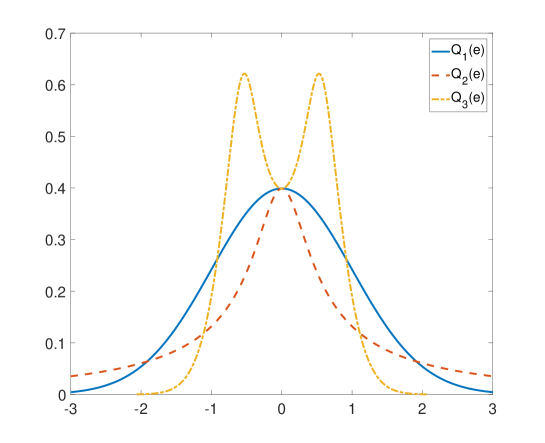
Figure 1: The figure plots probability density functions of $\varepsilon=Q_{j}(e)$, $j=1,2,3$, where $e\sim N(0,1)$ and $Q_{1}(e)=e$, $Q_{2}(e)=e+e^{3}$, and $Q_{3}(e)=(e+e^{3})/(1+2e^{2})$. All three probability density functions are allowed by Assumption 3.

Assumption 4 (Candidate set).

The candidate set $\Lambda_{n}$ takes the following form: $\Lambda_{n}=\{C_{1}a^{l}\colon l=0,1,2,\dots;\ a^{l}\geq c_{1}/n\}$.

It is known from [13] that the optimal rate of convergence of the Lasso estimator is achieved when $\lambda$ is of order $(\log p/n)^{1/2}$. Since under Assumption 2, we have $\log p=o(n)$, it follows that our choice of the candidate set $\Lambda_{n}$ in Assumption 4 makes sure that there are some $\lambda$’s in the candidate set $\Lambda_{n}$ that would yield the Lasso estimator with the optimal rate of convergence in the prediction norm. Note also that Assumption 4 allows for a rather large candidate set $\Lambda_{n}$ of values of $\lambda$; in particular, the largest value, $C_{1}$, can be set arbitrarily large and the smallest value, $c_{1}/n$, converges to zero rather fast. In fact, the only two conditions that we need from Assumption 4 is that $\Lambda_{n}$ contains a “good” value of $\lambda$, say $\bar{\lambda}_{0}$, such that the subsample Lasso estimators $\widehat{\beta}_{-k}(\bar{\lambda}_{0})$ satisfy the bound (10) in Lemma 7.2 with probability $1-Cn^{-c}$ and that $|\Lambda_{n}|\leq C\log n$, where $c$ and $C$ are some constants. Thus, we could for example set $\Lambda_{n}=\{a^{l}\colon l=\dots,-2,-1,0,1,2,\dots;\ a^{-l}\leq n^{C_{1}},\ a^{l}\leq n^{C_{1}}\}$.

Assumption 5 (Dataset partition).

The dataset partition $\{I_{k}\}_{k=1}^{K}$ is such that for all $k=1,\dots,K$, we have $n_{k}/n\geq c_{1}$, where $n_{k}=|I_{k}|$.

Assumption 5 is mild and is typically imposed in the literature on $K$-fold cross-validation. This assumption ensures that the subsamples $I_{k}$ are balanced in the sample size.

4 Main Results

Our first main result in this paper gives a non-asymptotic estimation error bound for the cross-validated Lasso estimator $\widehat{\beta}(\widehat{\lambda})$ in the prediction norm.

Theorem 4.1 (Prediction Norm Bound).

Suppose that Assumptions 1 – 5 hold. Then for any $\alpha\in(0,1)$,

$$\|\widehat{\beta}(\widehat{\lambda})-\beta\|_{2,n}\leq\sqrt{\frac{Cs\log(p/\alpha)}{n}}\times\sqrt{\log(pn)+s^{-1}\log^{r+1}n}$$

with probability at least $1-\alpha-Cn^{-c}$, where $c,C>0$ are constants depending only on $c_{1}$, $C_{1}$, $K$, $a$, $q$, and $r$.

Remark 4.1 (Near-rate-optimality of cross-validated Lasso estimator in prediction norm).

The results in [13] imply that under the assumptions of Theorem 4.1, setting $\lambda=\lambda^{\ast}=(C\log p/n)^{1/2}$ for sufficiently large constant $C$, which depends on the distribution of $\varepsilon$, gives the Lasso estimator $\widehat{\beta}(\lambda^{\ast})$ satisfying $\|\widehat{\beta}(\lambda^{\ast})-\beta\|_{2,n}=O_{P}((s\log p/n)^{1/2})$, and it follows from [34] that this is the optimal rate of convergence (in the minimax sense) for the estimators of $\beta$ in the model (1). Therefore, Theorem 4.1 implies that the cross-validated Lasso estimator $\widehat{\beta}(\widehat{\lambda})$ has the fastest possible rate of convergence in the prediction norm up to the small $(\log(pn)+s^{-1}\log^{r+1}n)^{1/2}$ factor. Note, however, that implementing the cross-validated Lasso estimator does not require knowledge of the distribution of $\varepsilon$, which makes this estimator attractive in practice. In addition, simulation evidence suggests that $\widehat{\beta}(\widehat{\lambda})$ often outperforms $\widehat{\beta}(\lambda^{\ast})$, which is one of the main reasons why cross-validation is typically recommended as a method to choose $\lambda$. The rate of convergence following from Theorem 4.1 is also very close to the oracle rate of convergence, $(s/n)^{1/2}$, that could be achieved by the OLS estimator if we knew the set of covariates having non-zero coefficients; see, for example, [11]. $\blacksquare$

Remark 4.2 (On the proof of Theorem 4.1).

One of the main steps in [13] is to show that outside of the event

$$\lambda<c\max_{1\leq j\leq p}\left|\frac{1}{n}\sum_{i=1}^{n}X_{ij}\varepsilon_{i}\right|,$$ (6)

where $c>2$ is some constant, the Lasso estimator $\widehat{\beta}(\lambda)$ satisfies the bound $\|\widehat{\beta}(\lambda)-\beta\|_{2,n}\leq C\lambda\sqrt{s}$, where $C$ is a constant. Thus, to obtain the Lasso estimator with a fast rate of convergence, it suffices to choose $\lambda$ such that it is small enough but the event (6) holds with at most small probability. The choice $\lambda=\lambda^{\ast}$ described in Remark 4.1 satisfies these two conditions. The difficulty with cross-validation, however, is that, as we demonstrate in Section 6 via simulations, it typically yields a rather small value of $\lambda$, so that the event (6) with $\lambda=\widehat{\lambda}$ holds with non-trivial (in fact, large) probability even in large samples, and little is known about properties of the Lasso estimator $\widehat{\beta}(\lambda)$ when the event (6) does not hold, which is perhaps one of the main reasons why there are only few results on the cross-validated Lasso estimator in the literature. We therefore take a different approach. First, we use the fact that $\widehat{\lambda}$ is the cross-validation choice of $\lambda$ to derive bounds on $\|\widehat{\beta}_{-k}(\widehat{\lambda})-\beta\|_{2}$ for the subsample Lasso estimators $\widehat{\beta}_{-k}(\widehat{\lambda})$ defined in (3). Second, we use the degrees of freedom formula of [49] and [42] to show that these estimators are sparse and to derive bounds on $\|\widehat{\beta}_{-k}(\widehat{\lambda})-\beta\|_{1}$ and $\|\widehat{\beta}_{-k}(\widehat{\lambda})-\beta\|_{2,n}$. Third, we use the two point inequality stating that for all $b\in\mathbb{R}^{p}$ and $\lambda>0$,

$$\|\widehat{\beta}(\lambda)-b\|_{2,n}^{2}\leq\frac{1}{n}\sum_{i=1}^{n}(Y_{i}-X_{i}^{\prime}b)^{2}+\lambda\|b\|_{1}-\frac{1}{n}\sum_{i=1}^{n}(Y_{i}-X_{i}^{\prime}\widehat{\beta}(\lambda))^{2}-\lambda\|\widehat{\beta}(\lambda)\|_{1},$$

which can be found in [44], with $\lambda=\widehat{\lambda}$ and $b=(K-1)^{-1}\sum_{k=1}^{K}(n-n_{k})\widehat{\beta}_{-k}(\widehat{\lambda})/n$, a convex combination of the subsample Lasso estimators $\widehat{\beta}_{-k}(\widehat{\lambda})$, and derive a bound for its right-hand side using the definition of estimators $\widehat{\beta}_{-k}(\widehat{\lambda})$ and bounds on $\|\widehat{\beta}_{-k}(\widehat{\lambda})-\beta\|_{2}$ and $\|\widehat{\beta}_{-k}(\widehat{\lambda})-\beta\|_{1}$. Finally, we use the triangle inequality to obtain a bound on $\|\widehat{\beta}(\widehat{\lambda})-\beta\|_{2,n}$ from the bounds on $\|\widehat{\beta}(\widehat{\lambda})-b\|_{2,n}$ and $\|\widehat{\beta}_{-k}(\widehat{\lambda})-\beta\|_{2,n}$. The details of the proof can be found in Section 7. $\blacksquare$

Next, in order to obtain bounds on $\|\widehat{\beta}(\widehat{\lambda})-\beta\|_{1}$ and $\|\widehat{\beta}(\widehat{\lambda})-\beta\|_{2}$, we derive a sparsity bound for $\widehat{\beta}(\widehat{\lambda})$, that is, we show that the estimator $\widehat{\beta}(\widehat{\lambda})$ has relatively few non-zero components, at least with high-probability. Even though our sparsity bound is not immediately useful in applications itself, it will help us to translate the result in the prediction norm in Theorem 4.1 into the result in $L^{1}$ and $L^{2}$ norms in Theorem 4.3.

Theorem 4.2 (Sparsity Bound).

Suppose that Assumptions 1 – 5 hold. Then for any $\alpha\in(0,1)$,

$$\|\widehat{\beta}(\widehat{\lambda})\|_{0}\leq Cs\times\frac{(\log^{2}p)(\log n)(\log(pn)+s^{-1}\log^{r+1}n)}{\alpha}$$

with probability at least $1-\alpha-Cn^{-c}$, where $c,C>0$ are constants depending only on $c_{1}$, $C_{1}$, $K$, $a$, $q$, and $r$.

Remark 4.3 (On the sparsity bound).

[9] showed that outside of the event (6), the Lasso estimator $\widehat{\beta}(\lambda)$ satisfies the bound $\|\widehat{\beta}(\lambda)\|_{0}\leq Cs$, for some constant $C$, so that the number of covariates that have been mistakenly selected by the Lasso estimator is at most of the same order as the number of non-zero coefficients in the original model (1). As explained in Remark 4.2, however, cross-validation typically yields a rather small value of $\lambda$, so that the event (6) with $\lambda=\widehat{\lambda}$ holds with non-trivial (in fact, large) probability even in large samples, and it is typically the case that smaller values of $\lambda$ lead to the Lasso estimators $\widehat{\beta}(\lambda)$ with a larger number of non-zero coefficients. We therefore should not necessarily expect that the inequality $\|\widehat{\beta}(\widehat{\lambda})\|_{0}\leq Cs$ holds with large probability. In fact, it is well-known (from simulations) in the literature that the cross-validated Lasso estimator typically satisfies $\|\widehat{\beta}(\widehat{\lambda})\|_{0}\gg s$. Our theorem, however, shows that even though the event (6) with $\lambda=\widehat{\lambda}$ may hold with large probability, the number of non-zero components in the cross-validated Lasso estimator $\widehat{\beta}(\widehat{\lambda})$ may exceed $Cs$ only by the relatively small $(\log^{2}p)(\log n)(\log(pn)+s^{-1}\log^{r+1})$ factor. $\blacksquare$

With the help of Theorems 4.1 and 4.2, we immediately obtain the following bounds on the $L^{1}$ and $L^{2}$ norms of the estimation error of the cross-validated Lasso estimator, which is our second main result in this paper.

Theorem 4.3 ($L^{1}$ and $L^{2}$ Norm Bounds).

Suppose that Assumptions 1 – 5 hold. Then for any $\alpha\in(0,1)$,

$$\|\widehat{\beta}(\widehat{\lambda})-\beta\|_{2}\leq\sqrt{\frac{Cs\log(p/\alpha)}{n}}\times\sqrt{\log(pn)+s^{-1}\log^{r+1}n}$$

and

$$\|\widehat{\beta}(\widehat{\lambda})-\beta\|_{1}\leq\sqrt{\frac{Cs^{2}\log(p/\alpha)}{n}}\times\sqrt{\frac{(\log^{2}p)(\log n)(\log(pn)+s^{-1}\log^{r+1}n)^{2}}{\alpha}}$$

with probability at least $1-\alpha-Cn^{-c}$, where $c,C>0$ are constants depending only on $c_{1}$, $C_{1}$, $K$, $a$, $q$, and $r$.

Remark 4.4 (Near-rate-optimality of cross-validated Lasso estimator in $L^{1}\$and $L^{2}$ norms).

Like in Remark 4.1, the results in [13] imply that under the assumptions of Theorem 4.3, setting $\lambda=\lambda^{\ast}=(C\log p/n)^{1/2}$ for sufficiently large constant $C$ gives the Lasso estimator $\widehat{\beta}(\lambda^{\ast})$ satisfying $\|\widehat{\beta}(\lambda^{\ast})-\beta\|_{2}=O_{P}((s\log p/n)^{1/2})$ and $\|\widehat{\beta}(\lambda^{\ast})-\beta\|_{1}=O_{P}((s^{2}\log p/n)^{1/2})$, and one can use the methods from [34] to show that these rates are optimal. Therefore, the cross-validated Lasso estimator $\widehat{\beta}(\widehat{\lambda})$ has the fastest possible rate of convergence both in $L^{1}$ and in $L^{2}$ norms, up to small logarithmic factors. $\blacksquare$

Remark 4.5 (On the case with Gaussian noise).

Recall that whenever the conditional distribution of $\varepsilon$ given $X$ is Gaussian, we can take $r=0$ in Assumption 3. Thus, it follows from Theorems 4.1 and 4.3 that, in this case, we have

$$\|\widehat{\beta}(\widehat{\lambda})-\beta\|_{2,n}\vee\|\widehat{\beta}(\widehat{\lambda})-\beta\|_{2}\leq\sqrt{\frac{Cs\log(p/\alpha)}{n}}\times\sqrt{\log(pn)}$$

with probability at least $1-\alpha-Cn^{-c}$ for any $\alpha\in(0,1)$ and some constants $c,C>0$. Theorems 4.2 and 4.3 can also be used to obtain the sparsity and $L^{1}$ norm bounds in this case as well. However, the sparsity and $L^{1}$ norm bounds here can be improved using results in [6]. In particular, assuming that the conditional distribution of $\varepsilon$ given $X$ is $N(0,\sigma^{2})$ for some constant $\sigma>0$, it follows from Theorem 4.3 in [6] that for any $\lambda>0$,

$$\text{Var}(\|\widehat{\beta}(\lambda)\|_{0}\mid X_{1}^{n})\leq{\mathrm{E}}[\|\widehat{\beta}(\lambda)\|_{0}\mid X_{1}^{n}]\left(3+4\log\left(\frac{ep}{{\mathrm{E}}[\|\widehat{\beta}(\lambda)\|_{0}\mid X_{1}^{n}]}\right)\right).$$

Combining this result and the same arguments as those in the proofs of Theorems 4.2 and 4.3, with Chebyshev’s inequality replacing Markov’s inequality in the proof of Theorem 4.2, we have

$$\|\widehat{\beta}(\widehat{\lambda})\|_{0}\leq Cs\times\frac{(\log^{2}p)\log(pn)}{\sqrt{\alpha}}$$

and

$$\|\widehat{\beta}(\widehat{\lambda})-\beta\|_{1}\leq\sqrt{\frac{Cs^{2}\log(p/\alpha)}{n}}\times\frac{(\log p)\log(pn)}{\alpha^{1/4}}$$

with probability at least $1-\alpha-Cn^{-c}$. $\blacksquare$

The near-rate-optimality of the cross-validated Lasso estimator in Theorem 4.1 may be viewed as an in-sample prediction property since the prediction norm

$$\|\widehat{\beta}-\beta\|_{2,n}=\left(\frac{1}{n}\sum_{i=1}^{n}(X_{i}^{\prime}\widehat{\beta}-X_{i}^{\prime}\beta)^{2}\right)^{1/2}$$

evaluates estimation errors with respect to the observed data $X_{1},\dots,X_{n}$. In addition, we can define an out-of-sample prediction norm

$$\|\widehat{\beta}-\beta\|_{p,2,n}=\Big{(}{\mathrm{E}}\Big{[}(X^{\prime}\widehat{\beta}-X^{\prime}\beta)^{2}\mid(X_{i},Y_{i})_{i=1}^{n}\Big{]}\Big{)}^{1/2},$$

where $X$ is independent of $X_{1},\dots,X_{n}$. Using Theorems 4.2 and 4.3, we immediately obtain the following corollary on the estimation error of the cross-validated Lasso estimator in the out-of-sample prediction norm:

Corollary 4.1 (Out-of-Sample Prediction Norm Bounds).

Suppose that Assumptions 1 – 5 hold. Then for any $\alpha\in(0,1)$,

$$\|\widehat{\beta}(\widehat{\lambda})-\beta\|_{p,2,n}\leq\sqrt{\frac{Cs\log(p/\alpha)}{n}}\times\sqrt{\log(pn)+s^{-1}\log^{r+1}n}$$

with probability at least $1-\alpha-Cn^{-c}$, where $c,C>0$ are constants depending only on $c_{1}$, $C_{1}$, $K$, $a$, $q$, and $r$.

5 General Sparsity Bounds

As we mentioned in Remark 4.2, our analysis of the (full-sample) cross-validated Lasso estimator $\widehat{\beta}(\widehat{\lambda})$ requires understanding sparsity of the sub-sample cross-validated Lasso estimators $\widehat{\beta}_{-k}(\widehat{\lambda})$, that is, we need a sparsity bound showing that $\|\widehat{\beta}_{-k}(\widehat{\lambda})\|_{0}$, $k=1,\dots,K$, are sufficiently small, at least with high probability. Unfortunately, existing sparsity bounds are not good enough for our purposes because, as we discussed in Remark 4.3, they only apply outside of the event (6) and this event holds with non-trivial (in fact, large) probability if we set $\lambda=\widehat{\lambda}$. We therefore develop here two novel sparsity bounds. The crucial feature of our bounds is that they apply for all values of $\lambda$, both large and small, independently of whether (6) holds or not. Roughly speaking, the first bound shows, under mild conditions, that the Lasso estimator $\widehat{\beta}(\lambda)$ has to be sparse, at least with large probability, whenever it has small estimation error in the $L^{2}$ norm. The second bound shows, under somewhat stronger conditions, that the Lasso estimator $\widehat{\beta}(\lambda)$ has to be sparse, at least on average, whenever it has small estimation error in the prediction norm. Both bounds turn out useful in our analysis.

Theorem 5.1 (Sparsity Bound via Estimation Error in $L^{2}$ Norm).

Suppose that Assumption 3 holds and let $\bar{C}>0$ be some constant. Then for all $\lambda>0$ and $t\geq 1$,

$${\mathrm{P}}\left(\|\widehat{\beta}(\lambda)\|_{0}\leq Cts\log^{2}(pn)\left(\log^{r}n+\frac{n(\log^{2}n)\|\widehat{\beta}(\lambda)-\beta\|_{2}^{2}}{s\log(pn)}\right)\mid X_{1}^{n}\right)\\ \leq 1-\frac{2}{ts\log(pn)}-\frac{2}{n},$$

on the event $\sup_{\delta\in\mathcal{S}^{p}(s)}\|\delta\|_{2,n}\leq\bar{C}$, where $C>0$ is a constant depending only on $c_{1}$, $C_{1}$, $\bar{C}$, and $r$.

Theorem 5.2 (Sparsity Bound via Estimation Error in Prediction Norm).

Suppose that Assumption 3 holds and let $\bar{c},\bar{C}>0$ be some constants. Then for all $\lambda>0$,

$${\mathrm{E}}[\|\widehat{\beta}(\lambda)\|_{0}\mid X_{1}^{n}]\leq s+C(\log p)(nR_{n}(\lambda)^{2}+\log^{r}n)$$

on the event

$$\bar{c}\leq\inf_{\delta\in\mathcal{S}^{p}(J_{n}(\lambda))}\|\delta\|_{2,n}\quad\text{and}\quad\max_{1\leq j\leq p}\sqrt{\frac{1}{n}\sum_{i=1}^{n}X_{ij}^{2}}\leq\bar{C},$$ (7)

where

$$J_{n}(\lambda)=n^{1/2+c_{1}/8}(\sqrt{n}R_{n}(\lambda)+1),\ R_{n}(\lambda)={\mathrm{E}}[\|\widehat{\beta}(\lambda)-\beta\|_{2,n}\mid X_{1}^{n}],$$

and $C>0$ is a constant depending only on $c_{1}$, $C_{1}$, $\bar{c}$, $\bar{C}$, and $r$.

6 Simulations

In this section, we present results of our simulation experiments. The purpose of the experiments is to investigate finite-sample properties of the cross-validated Lasso estimator. In particular, we are interested in (i) comparing the estimation error of the cross-validated Lasso estimator in different norms to the Lasso estimator based on other choices of $\lambda$; (ii) studying sparsity properties of the cross-validated Lasso estimator; and (iii) estimating probability of the event (6) for $\lambda=\widehat{\lambda}$, the cross-validation choice of $\lambda$.

We consider two data generating processes (DGPs). In both DGPs, we simulate the vector of covariates $X=(X_{1},\dots,X_{p})^{\prime}$ from the Gaussian distribution with mean zero and variance-covariance matrix given by $E[X_{j}X_{k}]=\rho^{|j-k|}$ for all $j,k=1,\dots,p$ with $\rho=0.5$ and $0.75$. Also, we set $\beta=(1,-1,2,-2,0_{1\times(p-4)})^{\prime}$. We simulate $\varepsilon$ from the standard Gaussian distribution in DGP1 and from the uniform distribution on $[-3,3]$ in DGP2. For both DGPs, we take $\varepsilon$ to be independent of $X$. Further, for each DGP, we consider samples of size $n=100$ and $400$. For each DGP and each sample size, we consider $p=40$, $100$, and $400$. To construct the candidate set $\Lambda_{n}$ of values of the penalty parameter $\lambda$, we use Assumption 4 with $a=0.9$, $c_{1}=0.005$ and $C_{1}=500$. Thus, the set $\Lambda_{n}$ contains values of $\lambda$ ranging from $0.0309$ to $500$ when $n=100$ and from $0.0071$ to $500$ when $n=400$, that is, the set $\Lambda_{n}$ is rather large in both cases. In all experiments, we use 5-fold cross-validation ($K=5$). We repeat each experiment $5000$ times.

As a comparison to the cross-validated Lasso estimator, we consider the Lasso estimators with $\lambda$ chosen according to [38] and [4], i.e.,

$$\lambda=n^{-1/2}\sigma\sqrt{2\log p}\text{ and }\lambda=n^{-1/2}\sigma\sqrt{2\log(p/s)}$$

respectively. These Lasso estimators achieve the optimal convergence rate under the prediction norm (see, e.g., [38] and [4]). The noise level $\sigma$ and the true sparsity $s$ typically have to be estimated from the data but for simplicity we assume that both $\sigma$ and $s$ are known, so we set $\sigma=1$ and $s=4$ in DGP1, and $\sigma=\sqrt{3}$ and $s=4$ in DGP2. In what follows, these Lasso estimators are denoted as SZ-Lasso and B-Lasso estimators respectively, and the cross-validated Lasso estimator is denoted as CV-Lasso.

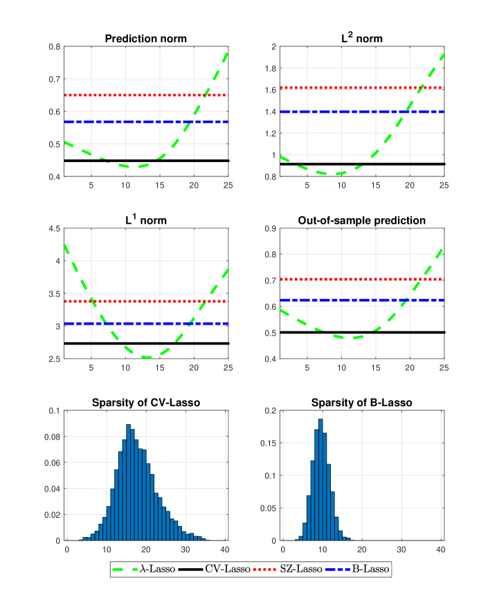
Figure 2: DGP1, $n=100$, $p=40$, and $\rho=0.75$. The top-left, top-right, middle-left, and middle-right panels show the mean of estimation error of Lasso estimators in the prediction, $L^{2}$, $L^{1}$, and out-of-sample prediction norms. The dashed line represents the mean of estimation error of the Lasso estimator as a function of $\lambda$ (we perform the Lasso estimator for each value of $\lambda$ in the candidate set $\Lambda_{n}$; we sort the values in $\Lambda_{n}$ from the smallest to the largest, and put the order of $\lambda$ on the horizontal axis; we only show the results for values of $\lambda$ up to order 25 as these give the most meaningful comparisons). The solid, dotted, and dashed-dotted horizontal lines represent the mean of the estimation error of the CV-Lasso, SZ-Lasso, and B-Lasso estimators, respectively.

Figure 2 contains simulation results for DGP1 with $n=100$, $p=40$ and $\rho=0.75$. The first four (that is, the top-left, top-right, middle-left and middle-right) panels of Figure 2 present the mean of the estimation error of the Lasso estimators in the prediction, $L^{2}$, $L^{1}$, and out-of-sample prediction norms, respectively. The out-of-sample prediction norm is defined as $\left\|b\right\|_{p,2,n}=({\mathrm{E}}[(X^{\prime}b)^{2}])^{1/2}$ for all $b\in\mathbb{R}^{p}$. In these panels, the dashed line represents the mean of estimation error of the Lasso estimator as a function of $\lambda$ (we perform the Lasso estimator for each value of $\lambda$ in the candidate set $\Lambda_{n}$; we sort the values in $\Lambda_{n}$ from the smallest to the largest, and put the order of $\lambda$ on the horizontal axis; we only show the results for values of $\lambda$ up to order 25 as these give the most meaningful comparisons). This estimator is denoted as $\lambda$-Lasso. The solid, dotted and dashed-dotted horizontal lines represent the mean of the estimation error of CV-Lasso, SZ-Lasso, and B-Lasso, respectively.

From the top four panels of Figure 2, we see that estimation error of CV-Lasso is only slightly above the minimum of the estimation error over all possible values of $\lambda$ not only in the prediction and $L^{2}$ norms but also in the $L^{1}$ norm. In comparison, SZ-Lasso and B-Lasso tend to have larger estimation error in all four norms.

The bottom-left and bottom-right panels of Figure 2 depict the histograms for the numbers of non-zero coefficients of the CV-Lasso estimator and B-Lasso estimator respectively. Overall, these panels suggest that the CV-Lasso estimator tends to select too many covariates: the number of selected covariates with large probability varies between $5$ and $30$ even though there are only 4 non-zero coefficients in the true model. The B-Lasso estimator is more sparse than the CV-Lasso estimator: it selects around $5$ to $15$ covariates with large probability.

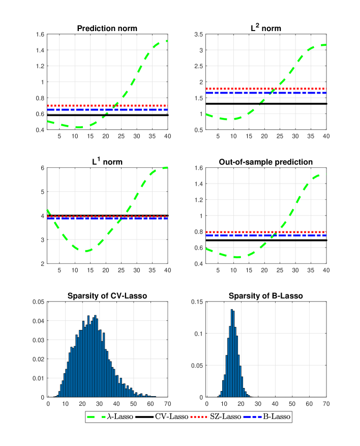
Figure 3: DGP1, $n=100$, $p=400$, and $\rho=0.75$. The top-left, top-right, middle-left, and middle-right panels show the mean of estimation error of Lasso estimators in the prediction, $L^{2}$, $L^{1}$, and out-of-sample prediction norms. The dashed line represents the mean of estimation error of the Lasso estimator as a function of $\lambda$ (we perform the Lasso estimator for each value of $\lambda$ in the candidate set $\Lambda_{n}$; we sort the values in $\Lambda_{n}$ from the smallest to the largest, and put the order of $\lambda$ on the horizontal axis; we only show the results for values of $\lambda$ up to order 25 as these give the most meaningful comparisons). The solid, dotted, and dashed-dotted horizontal lines represent the mean of the estimation error of the CV-Lasso, SZ-Lasso, and B-Lasso estimators, respectively.

Figure 3 includes the simulation results for DGP1 when $n=100$, $p=400$ and $\rho=0.75$. The estimation errors of the Lasso estimators are inflated when $p$ is much bigger than the sample size. The estimation error of CV-Lasso under the prediction norm is increased from $0.4481$ to $0.7616$ when $p$ is increased from $40$ to $400$, although it remains the best compared with SZ-Lasso and B-Lasso estimators. Similar phenomena are observed for the estimation error under the $L^{2}$ norm and the out-of-sample prediction norm. On the other hand, the estimation error of the CV-Lasso is slightly larger than the SZ-Lasso and B-Lasso under the $L^{1}$ norm. For the sparsity of the Lasso estimators, the CV-Lasso is much less sparse than the B-Lasso: it selects around $5$ to $50$ covariates with large probability while the B-Lasso only selects $8$ to $22$ covariates with large probability.

For all other experiments, the simulation results on the mean of estimation error of the Lasso estimators can be found in Table 1. For simplicity, we only report the minimum over $\lambda\in\Lambda_{n}$ of mean of the estimation error of $\lambda$-Lasso and the mean of the estimation error of B-Lasso in Table 1. The results in Table 1 confirm findings in Figure 2 and Figure 3: the mean of the estimation error of CV-Lasso is close to the minimum mean of the estimation errors of the $\lambda$-Lasso estimators under both DGPs for all combinations of $n$, $p$ and $\rho$ considered in all three norms. Their difference becomes smaller when the sample size $n$ increases. The mean of the estimation error of B-Lasso is larger than that of CV-Lasso in cases when $p$ is relatively small or the regressors $X$ have strong correlation, while the B-Lasso has smaller estimation error when $p$ is much larger than $n$ and the regressors $X$ are weakly correlated. When the correlations of the regressors $X$ become stronger and the largest eigenvalue of ${\mathrm{E}}[XX^{\prime}]$ becomes bigger, the mean of the estimation error of the CV-Lasso estimator is slightly enlarged and is much less effected compared with the B-Lasso estimator. For example, in DGP1 with $n=100$ and $p=40$, the mean of estimation error of CV-Lasso estimator increases $5.39\%$ when $\rho$ is changed from $0.5$ to $0.75$ (and the largest eigenvalue of ${\mathrm{E}}[XX^{\prime}]$ increases from $2.97$ to $6.64$), while the B-Lasso estimator has a $28\%$ increase.

Table 2 reports model selection results for the cross-validated Lasso estimator. More precisely, the table shows probabilities for the number of non-zero coefficients of the cross-validated Lasso estimator hitting different brackets. Overall, the results in Table 2 confirm findings in Figure 2 and Figure 3: the cross-validated Lasso estimator tends to select too many covariates. The probability of selecting larger models tends to increase with $p$ but decreases with $n$.

Table 3 provides information on the finite-sample distribution of the ratio of the maximum score $\max_{1\leq j\leq p}|n^{-1}\sum_{i=1}^{n}X_{ij}\varepsilon_{i}|$ over $\widehat{\lambda}$, the cross-validation choice of $\lambda$. More precisely, the table shows probabilities for this ratio hitting different brackets. From Table 3, we see that this ratio is above 0.5 with large probability in all cases and in particular this probability exceeds 99% in most cases. Hence, (6) with $\lambda=\widehat{\lambda}$ holds with large probability, meaning that deriving the rate of convergence of the cross-validated Lasso estimator requires new arguments since existing arguments only work for the case when (6) does not hold; see discussion in Remark 4.2 above.

7 Proofs for Section 4

In this section, we prove Theorems 4.1, 4.2, and 4.3 and Corollary 4.1. Since the proofs are long, we start with a sequence of preliminary lemmas in Subsection 7.1 and give the actual proofs of the theorems and the corollary in Subsections 7.2, 7.3, 7.4, and 7.5, respectively.

For convenience, we use the following additional notation. For $k=1,\dots,K$, we denote

$$\|\delta\|_{2,n,k}=\bigg{(}\frac{1}{n_{k}}\sum_{i\in I_{k}}(X_{i}^{\prime}\delta)^{2}\bigg{)}^{1/2}\ \text{ and }\ \|\delta\|_{2,n,-k}=\bigg{(}\frac{1}{n-n_{k}}\sum_{i\notin I_{k}}(X_{i}^{\prime}\delta)^{2}\bigg{)}^{1/2}$$

for all $\delta\in\mathbb{R}^{p}$. We use $c$ and $C$ to denote strictly positive constants that can change from place to place but that can be chosen to depend only on $c_{1}$, $C_{1}$, $K$, $a$, $q$, and $r$. We use the notation $a_{n}\lesssim b_{n}$ if $a_{n}\leq Cb_{n}$. Moreover, for $\delta\in\mathbb{R}^{p}$ and $M\subset\{1,\dots,p\}$, we use $\delta_{M}$ to denote the vector in $\mathbb{R}^{|M|}$ consisting of all elements of $\delta$ corresponding to indices in $M$.

7.1 Preliminary Lemmas

Here, we collect preliminary lemmas that help to prove Theorems 4.1–4.3.

Lemma 7.1.

Suppose that Assumptions 1 and 2 are satisfied and denote $\ell_{n}=\sqrt{sn^{1+c_{1}/2}}\log(pn)$. Then

$$\sup_{\theta\in\mathcal{S}^{p}(\ell_{n})}\left|\frac{1}{n}\sum_{i=1}^{n}(X_{i}^{\prime}\theta)^{2}-{\mathrm{E}}[(X^{\prime}\theta)^{2}]\right|\leq Cn^{-c}$$ (8)

with probability at least $1-Cn^{-c}$, where $c$, $C>0$ are some constants depending only on $c_{1}$, $C_{1}$, and $q$.

Proof.

In this proof, $c$ and $C$ are strictly positive constants that depend only on $c_{1}$, $C_{1}$, and $q$ but their values can change from place to place. By Jensen’s inequality and the definition of $M_{n}$ in (5),

$$K_{n} :=\left({\mathrm{E}}\left[\max_{1\leq i\leq n}\max_{1\leq j\leq p}|X_{ij}|^{2}\right]\right)^{1/2}$$

$$\leq\left({\mathrm{E}}\left[\max_{1\leq i\leq n}\max_{1\leq j\leq p}|X_{ij}|^{q}\right]\right)^{1/q}\leq n^{1/q}M_{n}.$$ (9)

Therefore, given that $\ell_{n}\leq Cn^{1-c}$ by Assumptions 1(a) and 2, which implies $\log\ell_{n}\leq C\log n$, it follows that

$$\delta_{n}:=K_{n}\sqrt{\ell_{n}\log p/n}\left(1+(\log\ell_{n})(\log n)^{1/2}\right)\leq Cn^{-c}$$

by Assumption 2; here, Assumption 1(a) is used only to verify that $M_{n}\geq c$. Also, denoting $\ell_{n,0}=n^{2/q+c_{1}}M_{n}^{2}s\log^{3}(pn)$,

$$\sup_{\theta\in\mathcal{S}^{p}(\ell_{n})}{\mathrm{E}}[(X^{\prime}\theta)^{2}]\leq\frac{2(\ell_{n}+\ell_{n,0})}{\ell_{n,0}}\sup_{\theta\in\mathcal{S}^{p}(\ell_{n,0})}{\mathrm{E}}[(X^{\prime}\theta)^{2}]\leq\frac{C(\ell_{n}+\ell_{n,0})}{\ell_{n,0}}$$

by Lemma 9 in [8] and Assumption 1(b). Thus,

$$\delta_{n}\sup_{\theta\in\mathcal{S}^{p}(\ell_{n})}\left({\mathrm{E}}[(X^{\prime}\theta)^{2}]\right)^{1/2}\leq Cn^{-c}$$

by Assumption 2. Therefore, it follows from Lemma 9.3 that

$${\mathrm{E}}\left[\sup_{\theta\in\mathcal{S}^{p}(\ell_{n})}\left|\frac{1}{n}\sum_{i=1}^{n}(X_{i}^{\prime}\theta)^{2}-{\mathrm{E}}[(X^{\prime}\theta)^{2}]\right|\right]\leq Cn^{-c}.$$

The asserted claim follows from combining this bound and Markov’s inequality. $\blacksquare$

Lemma 7.2.

Under Assumptions 1–5, there exists $\bar{\lambda}_{0}=\bar{\lambda}_{n,0}\in\Lambda_{n}$, possibly depending on $n$, such that for all $k=1,\dots,K$, we have $\|\widehat{\beta}_{-k}(\bar{\lambda}_{0})\|_{0}\lesssim s$ and, in addition,

$$\|\widehat{\beta}_{-k}(\bar{\lambda}_{0})-\beta\|_{2}^{2}\lesssim\frac{s\log(pn)}{n}\ \text{ and }\ \|\widehat{\beta}_{-k}(\bar{\lambda}_{0})-\beta\|_{1}^{2}\lesssim\frac{s^{2}\log(pn)}{n}$$ (10)

with probability at least $1-Cn^{-c}$.

Remark 7.1.

The result in this lemma is essentially well-known but we provide a short proof here for completeness.

Proof.

Let $T=\{j\in\{1,\dots,p\}\colon\beta_{j}\neq 0\}$ and $T^{c}=\{1,\dots,p\}\backslash T$. Fix $k=1,\dots,K$ and denote

$$Z_{k}=\frac{1}{n-n_{k}}\sum_{i\notin I_{k}}X_{i}\varepsilon_{i}$$

and

$$\kappa_{k}=\inf\left\{\frac{\sqrt{s}\|\delta\|_{2,n,-k}}{\|\delta_{T}\|_{1}}\colon\ \delta\in\mathbb{R}^{p},\ \|\delta_{T^{c}}\|_{1}<3\|\delta_{T}\|_{1}\right\}.$$

To prove the asserted claims, we will apply Theorem 1 in [8] that shows that for any $\lambda\in\Lambda_{n}$, on the event $\lambda\geq 4\|Z_{k}\|_{\infty}$, we have

$$\|\widehat{\beta}_{-k}(\lambda)-\beta\|_{2,n,-k}\leq\frac{3\lambda\sqrt{s}}{2\kappa_{k}}.$$ (11)

To use this bound, we show that there exist $c>0$, $C>0$, and $\bar{\lambda}_{0}=\bar{\lambda}_{n,0}\in\Lambda_{n}$, possibly depending on $n$, such that

$$P(\kappa_{k}<c)\leq Cn^{-c},\ P\left(\bar{\lambda}_{0}<4\|Z_{k}\|_{\infty}\right)\leq Cn^{-c},\ \bar{\lambda}_{0}\lesssim\left(\frac{\log(pn)}{n}\right)^{1/2}.$$ (12)

To prove the first claim in (12), note that

$$1\lesssim\|\delta\|_{2,n,-k}\lesssim 1$$ (13)

with probability at least $1-Cn^{-c}$ uniformly over all $\delta\in\mathbb{R}^{p}$ such that $\|\delta\|_{2}=1$ and $\|\delta_{T^{c}}\|_{0}\leq s\log n$ by Lemma 7.1 and Assumptions 1, 2 and 5. Hence, the first claim in (12) follows from Lemma 10 in [8] applied with $m$ there equal to $s\log n$ here.

To prove the second and the third claims in (12), note that we have $\max_{1\leq j\leq p}\sum_{i\notin I_{k}}{\mathrm{E}}[|X_{ij}\varepsilon_{i}|^{2}]\lesssim n$ by Assumptions 1(b) and 3. Also,

$$\Big{(}{\mathrm{E}}\Big{[}\max_{1\leq i\leq n}\max_{1\leq j\leq p}|X_{ij}\varepsilon_{i}|^{2}\Big{]}\Big{)}^{1/2}\leq\Big{(}{\mathrm{E}}\Big{[}\max_{1\leq i\leq n}\max_{1\leq j\leq p}|X_{ij}\varepsilon_{i}|^{q}\Big{]}\Big{)}^{1/q}\lesssim n^{1/q}M_{n}.$$

Thus, by Lemma 9.1 and Assumption 2,

$${\mathrm{E}}\Big{[}(n-n_{k})\|Z_{k}\|_{\infty}\Big{]}\lesssim\sqrt{n\log p}+n^{1/q}M_{n}\log p\lesssim\sqrt{n\log p}.$$

Hence, applying Lemma 9.2 with $t=(n\log n)^{1/2}$ and $Z$ there replaced by $(n-n_{k})\|Z_{k}\|_{\infty}$ here and noting that $nM_{n}^{q}/(n\log n)^{q/2}\leq Cn^{-c}$ by Assumption 2 implies that

$$\|Z_{k}\|_{\infty}\lesssim\left(\frac{\log(pn)}{n}\right)^{1/2}$$

with probability at least $1-Cn^{-c}$. Hence, noting that $\log^{4}(pn)\leq Cn$ by Assumptions 1(a) and 2, it follows from Assumption 4 that there exists $\bar{\lambda}_{0}\in\Lambda_{n}$ such that the second and the third claims in (12) hold. By (11), this $\bar{\lambda}_{0}$ satisfies the following bound:

$$P\left(\|\widehat{\beta}_{-k}(\bar{\lambda}_{0})-\beta\|_{2,n,-k}^{2}>\frac{Cs\log(pn)}{n}\right)\leq Cn^{-c}.$$ (14)

Now, to prove the asserted claims, note that using (12) and (13) and applying Theorem 2 in [8] with $m=s\log n$ there shows that $\|\widehat{\beta}_{-k}(\bar{\lambda}_{0})\|_{0}\lesssim s$ with probability at least $1-Cn^{-c}$. Hence,

$$\|\widehat{\beta}_{-k}(\bar{\lambda}_{0})-\beta\|_{1}^{2} \lesssim s\|\widehat{\beta}_{-k}(\bar{\lambda}_{0})-\beta\|_{2}^{2}$$

$$\lesssim s\|\widehat{\beta}_{-k}(\bar{\lambda}_{0})-\beta\|_{2,n,-k}^{2}\lesssim\frac{s^{2}\log(pn)}{n}$$

again with probability at least $1-Cn^{-c}$, where the second inequality follows from (13), and the third one from (14). This gives all asserted claims and completes the proof of the lemma. $\blacksquare$

Lemma 7.3.

Under Assumptions 1–5, we have for all $k=1,\dots,K$ that

$$\|\widehat{\beta}_{-k}(\bar{\lambda}_{0})-\beta\|_{2,n,k}^{2}\lesssim\frac{s\log(pn)}{n}$$

with probability $1-Cn^{-c}$ for $\bar{\lambda}_{0}$ defined in Lemma 7.2.

Remark 7.2.

We thank one of the anonymous referees for suggesting the proof below. The suggestion relaxes the condition $s^{2}/n=o(1)$ in our early proof to $s/n=o(1)$, up to some log factors. $\blacksquare$

Proof.

Fix $k=1,\dots,K$ and denote $\widehat{\beta}=\widehat{\beta}_{-k}(\bar{\lambda}_{0})$. By Lemma 7.2, $\|\widehat{\beta}\|_{0}\lesssim s$ with probability at least $1-Cn^{-c}$. Hence,

$$\|\widehat{\beta}-\beta\|_{2,n,k}^{2} \lesssim(\widehat{\beta}-\beta)^{\prime}{\mathrm{E}}[XX^{\prime}](\widehat{\beta}-\beta)+\|\widehat{\beta}-\beta\|_{2}^{2}\lesssim\|\widehat{\beta}-\beta\|_{2}^{2}\lesssim\frac{s\log(pn)}{n}$$

with probability at least $1-Cn^{-c}$, where the first inequality follows from Lemma 7.1 and Assumption 5, the second from Assumption 1(b), and the third from Lemma 7.2. The asserted claim follows. $\blacksquare$

Lemma 7.4.

Under Assumptions 1–5, we have for all $k=1,\dots,K$ that

$$\|\widehat{\beta}_{-k}(\widehat{\lambda})-\beta\|_{2,n,k}^{2}\lesssim\frac{s\log(pn)}{n}+\frac{\log^{r+1}n}{n}$$

with probability at least $1-Cn^{-c}$.

Proof.

By the definition of $\widehat{\lambda}$ in (4),

$$\sum_{k=1}^{K}\sum_{i\in I_{k}}(Y_{i}-X_{i}^{\prime}\widehat{\beta}_{-k}(\widehat{\lambda}))^{2}\leq\sum_{k=1}^{K}\sum_{i\in I_{k}}(Y_{i}-X_{i}^{\prime}\widehat{\beta}_{-k}(\bar{\lambda}_{0}))^{2}$$

for $\bar{\lambda}_{0}$ defined in Lemma 7.2. Therefore,

$$\sum_{k=1}^{K}n_{k}\|\widehat{\beta}_{-k}(\widehat{\lambda})-\beta\|_{2,n,k}^{2} \leq\sum_{k=1}^{K}n_{k}\|\widehat{\beta}_{-k}(\bar{\lambda}_{0})-\beta\|_{2,n,k}^{2}$$

$$\quad+2\sum_{k=1}^{K}\sum_{i\in I_{k}}\varepsilon_{i}X_{i}^{\prime}(\widehat{\beta}_{-k}(\widehat{\lambda})-\widehat{\beta}_{-k}(\bar{\lambda}_{0})).$$

Further, for all $k=1,\dots,K$, denote $D_{k}=\{(X_{i},Y_{i})_{i\notin I_{k}},(X_{i})_{i\in I_{k}}\}$ and

$$Z_{k}=\max_{\lambda\in\Lambda_{n}}\left|\frac{\sum_{i\in I_{k}}\varepsilon_{i}X_{i}^{\prime}(\widehat{\beta}_{-k}(\lambda)-\widehat{\beta}_{-k}(\bar{\lambda}_{0}))}{\sqrt{n_{k}}\|\widehat{\beta}_{-k}(\lambda)-\widehat{\beta}_{-k}(\bar{\lambda}_{0})\|_{2,n,k}}\right|.$$

Then by Lemma 9.1 and Assumptions 3 and 4, we have that ${\mathrm{E}}[Z_{k}\mid D_{k}]\lesssim\sqrt{\log\log n}+M_{n,k}\log\log n$, where

$$M_{n,k} =\left({\mathrm{E}}\left[\max_{\lambda\in\Lambda_{n}}\max_{i\in I_{k}}\frac{(\varepsilon_{i}X_{i}^{\prime}(\widehat{\beta}_{-k}(\lambda)-\widehat{\beta}_{-k}(\bar{\lambda}_{0})))^{2}}{n_{k}\|\widehat{\beta}_{-k}(\lambda)-\widehat{\beta}_{-k}(\bar{\lambda}_{0})\|_{2,n,k}^{2}}\mid D_{k}\right]\right)^{1/2}$$

$$\leq\left({\mathrm{E}}\left[\max_{\lambda\in\Lambda_{n}}\max_{i\in I_{k}}\frac{|\varepsilon_{i}X_{i}^{\prime}(\widehat{\beta}_{-k}(\lambda)-\widehat{\beta}_{-k}(\bar{\lambda}_{0}))|^{u}}{n_{k}^{u/2}\|\widehat{\beta}_{-k}(\lambda)-\widehat{\beta}_{-k}(\bar{\lambda}_{0})\|_{2,n,k}^{u}}\mid D_{k}\right]\right)^{1/u}$$

$$\leq\left({\mathrm{E}}\left[\sum_{\lambda\in\Lambda_{n}}\sum_{i\in I_{k}}\frac{|\varepsilon_{i}X_{i}^{\prime}(\widehat{\beta}_{-k}(\lambda)-\widehat{\beta}_{-k}(\bar{\lambda}_{0}))|^{u}}{n_{k}^{u/2}\|\widehat{\beta}_{-k}(\lambda)-\widehat{\beta}_{-k}(\bar{\lambda}_{0})\|_{2,n,k}^{u}}\mid D_{k}\right]\right)^{1/u}$$

for any $u\geq 2$. In turn, the last expression is bounded from above by

$$C\left((u(1+r))^{u(1+r)/2}\log n\right)^{1/u}$$

since (i) ${\mathrm{E}}[|\varepsilon_{i}|^{u}\mid D_{k}]\leq C^{u}{\mathrm{E}}[(1+|e|+|e|^{r+1})^{u}]\leq C^{u}(u(1+r))^{u(1+r)/2}$ under Assumption 3 and (ii) for any sequence $(a_{i})_{i\in I_{k}}$ in $\mathbb{R}$, we have $\sum_{i\in I_{k}}|a_{i}|^{u}\leq(\sum_{i\in I_{k}}|a_{i}|^{2})^{u/2}.$ Using this bound with $u=3$ (for example) gives ${\mathrm{E}}[Z_{k}\mid D_{k}]\lesssim\sqrt{\log n}$. In addition, using this bound with $u=\log n$, it follows from Lemma 9.2 that

$${\mathrm{P}}\Big{(}Z_{k}>2{\mathrm{E}}[Z_{k}\mid D_{k}]+C\sqrt{\log^{r+1}n}\mid D_{k}\Big{)}\leq Cn^{-c}.$$

Hence, $Z_{k}\lesssim\sqrt{\log^{r+1}n}$ with probability at least $1-Cn^{-c}$, and so, with the same probability,

$$\left|\sum_{i\in I_{k}}\varepsilon_{i}X_{i}^{\prime}(\widehat{\beta}_{-k}(\widehat{\lambda})-\widehat{\beta}_{-k}(\bar{\lambda}_{0}))\right|\lesssim\sqrt{n\log^{r+1}n}\|\widehat{\beta}_{-k}(\widehat{\lambda})-\widehat{\beta}_{-k}(\bar{\lambda}_{0})\|_{2,n,k}.$$

Therefore, since $n_{k}/n\geq c_{1}$ by Assumption 5, we have with the same probability that

$$\sum_{k=1}^{K}\|\widehat{\beta}_{-k}(\widehat{\lambda})-\beta\|_{2,n,k}^{2} \lesssim\sum_{k=1}^{K}\|\widehat{\beta}_{-k}(\bar{\lambda}_{0})-\beta\|_{2,n,k}^{2}$$

$$\quad+\sqrt{\frac{\log^{r+1}n}{n}}\sum_{k=1}^{K}\|\widehat{\beta}_{-k}(\widehat{\lambda})-\widehat{\beta}_{-k}(\bar{\lambda}_{0})\|_{2,n,k},$$

and thus, by the triangle inequality,

$$\|\widehat{\beta}_{-\widehat{k}}(\widehat{\lambda})-\widehat{\beta}_{-\widehat{k}}(\bar{\lambda}_{0})\|_{2,n,\widehat{k}}^{2} \lesssim\sum_{k=1}^{K}\|\widehat{\beta}_{-k}(\bar{\lambda}_{0})-\beta\|_{2,n,k}^{2}$$

$$\quad+\sqrt{\frac{\log^{r+1}n}{n}}\|\widehat{\beta}_{-\widehat{k}}(\widehat{\lambda})-\widehat{\beta}_{-\widehat{k}}(\bar{\lambda}_{0})\|_{2,n,\widehat{k}},$$

where $\widehat{k}$ is a value of $k=1,\dots,K$ that maximizes $\|\widehat{\beta}_{-k}(\widehat{\lambda})-\widehat{\beta}_{-k}(\bar{\lambda}_{0})\|_{2,n,k}$. Therefore, by Lemma 7.3,

$$\|\widehat{\beta}_{-\widehat{k}}(\widehat{\lambda})-\widehat{\beta}_{-\widehat{k}}(\bar{\lambda}_{0})\|_{2,n,\widehat{k}}^{2}\lesssim\frac{s\log(pn)}{n}+\sqrt{\frac{\log^{r+1}n}{n}}\|\widehat{\beta}_{-\widehat{k}}(\widehat{\lambda})-\widehat{\beta}_{-\widehat{k}}(\bar{\lambda}_{0})\|_{2,n,\widehat{k}},$$

and thus, for all $k=1,\dots,K$,

$$\|\widehat{\beta}_{-k}(\widehat{\lambda})-\widehat{\beta}_{-k}(\bar{\lambda}_{0})\|_{2,n,k}^{2}\leq\|\widehat{\beta}_{-\widehat{k}}(\widehat{\lambda})-\widehat{\beta}_{-\widehat{k}}(\bar{\lambda}_{0})\|_{2,n,\widehat{k}}^{2}\lesssim\frac{s\log(pn)}{n}+\frac{\log^{r+1}n}{n},$$

again with probability at least $1-Cn^{-c}$. The asserted claim now follows from combining this bound with the triangle inequality and Lemma 7.3. This completes the proof of the lemma. $\blacksquare$

Lemma 7.5.

Under Assumptions 1 – 5, we have for all $k=1,\dots,K$ that

$$\|\widehat{\beta}_{-k}(\widehat{\lambda})-\beta\|_{2}^{2}\lesssim\frac{s\log(pn)}{n}+\frac{\log^{r+1}n}{n}$$

with probability at least $1-Cn^{-c}$.

Proof.

Fix $k=1,\dots,K$. For $\lambda\in\Lambda_{n}$, let $\delta_{\lambda}=(\widehat{\beta}_{-k}(\lambda)-\beta)/\|\widehat{\beta}_{-k}(\lambda)-\beta\|_{2}$ and observe that conditional on $(X_{i},Y_{i})_{i\notin I_{k}}$, $(\delta_{\lambda})_{\lambda\in\Lambda_{n}}$ is non-stochastic. Hence, by Lemma 8.1, Assumptions 1(a) and 5 and Chebyshev’s inequality applied conditional on $(X_{i},Y_{i})_{i\notin I_{k}}$, for any $\lambda\in\Lambda_{n}$, $(n_{k})^{-1}\sum_{i\in I_{k}}(X_{i}^{\prime}\delta_{\lambda})^{2}\geq c$ with probability at least $1-Cn^{-c}$, and so $\|\widehat{\beta}_{-k}(\lambda)-\beta\|_{2}^{2}\leq C\|\widehat{\beta}_{-k}(\lambda)-\beta\|_{2,n,k}^{2}$ with the same probability. Therefore, by Assumption 4 and the union bound, $\|\widehat{\beta}_{-k}(\widehat{\lambda})-\beta\|_{2}^{2}\leq C\|\widehat{\beta}_{-k}(\widehat{\lambda})-\beta\|_{2,n,k}^{2}$ with probability at least $1-Cn^{-c}$. The asserted claim follows from combining this inequality and Lemma 7.4. $\blacksquare$

Lemma 7.6.

Fix $k=1,\dots,K$ and denote

$$\Lambda_{n,k}(X_{1}^{n},T)=\left\{\lambda\in\Lambda_{n}\colon{\mathrm{E}}[\|\widehat{\beta}_{-k}(\lambda)-\beta\|_{2,n,-k}\mid X_{1}^{n}]\leq T\right\},\quad T>0.$$ (15)

Then under Assumptions 1 – 5, we have that $\widehat{\lambda}\in\Lambda_{n,k}(X_{1}^{n},T_{n})$ with probability at least $1-Cn^{-c}$, where

$$T_{n}=C\left(\frac{s\log(pn)}{n}+\frac{\log^{r+1}n}{n}\right)^{1/2}.$$ (16)

Proof.

Fix $k=1,\dots,K$ and note that by Assumption 1(b) and Lemma 7.1, $\sup_{\delta\in\mathcal{S}^{p}(s)}\|\delta\|_{2,n}\leq C$ with probability at least $1-Cn^{-c}$. Hence, by Lemma 7.5, Theorem 5.1, Assumption 4, and the union bound, $\|\widehat{\beta}_{-k}(\widehat{\lambda})\|_{0}\leq n^{c_{1}/4}s\log^{2}(pn)$ with probability at least $1-Cn^{-c}$. Further, by Assumption 2, $n^{c_{1}/4}s\log^{2}(pn)\leq\sqrt{sn^{1+c_{1}/2}}\log(pn)$ for all $n\geq n_{0}$ with $n_{0}$ depending only on $c_{1}$ and $C_{1}$, and so, by Assumption 1(b) and Lemma 7.1, $\|\widehat{\beta}_{-k}(\widehat{\lambda})-\beta\|_{2,n,-k}^{2}\lesssim\|\widehat{\beta}_{-k}(\widehat{\lambda})-\beta\|_{2}^{2}$ with probability at least $1-Cn^{-c}$. Combining this bound with Lemma 7.5 now gives

$${\mathrm{P}}\left(\|\widehat{\beta}_{-k}(\widehat{\lambda})-\beta\|_{2,n,-k}^{2}>C\left(\frac{s\log(pn)}{n}+\frac{\log^{r+1}n}{n}\right)\right)\leq Cn^{-c}.$$ (17)

Now,

$${\mathrm{P}}\left(\widehat{\lambda}\notin\Lambda_{n,k}(X_{1}^{n},T_{n})\right)\leq{\mathrm{P}}\left(\|\widehat{\beta}_{-k}(\widehat{\lambda})-\beta\|_{2,n,-k}>T_{n}/2\right)$$

$$\quad+{\mathrm{P}}\left(\max_{\lambda\in\Lambda_{n}}\left|\|\widehat{\beta}_{-k}(\lambda)-\beta\|_{2,n,-k}-{\mathrm{E}}[\|\widehat{\beta}_{-k}(\lambda)-\beta\|_{2,n,-k}\mid X_{1}^{n}]\right|>T_{n}/2\right),$$

where the first and the second terms on the right-hand side are at most $Cn^{-c}$ by (17) and Lemma 8.2 applied with $\kappa=\log n$, respectively, as long the constant $C$ in the definition of $T_{n}$ is large enough. The asserted claim follows. $\blacksquare$

Lemma 7.7.

For all $\lambda\in\Lambda_{n}$ and $b\in\mathbb{R}^{p}$, we have

$$\|\widehat{\beta}(\lambda)-b\|_{2,n}^{2}\leq\frac{1}{n}\sum_{i=1}^{n}(Y_{i}-X_{i}^{\prime}b)^{2}+\lambda\|b\|_{1}-\frac{1}{n}\sum_{i=1}^{n}(Y_{i}-X_{i}^{\prime}\widehat{\beta}(\lambda))^{2}-\lambda\|\widehat{\beta}(\lambda)\|_{1}.$$

Proof.

The result in this lemma is sometimes referred to as the two point inequality; see Section 2.4 in [44], where the proof is also provided. $\blacksquare$

7.2 Proof of Theorem 4.1

Throughout the proof, we can assume that $\alpha\in[1/n,e^{-2}]$ since the results for $\alpha>e^{-2}$ and $\alpha<1/n$ follow from the cases $\alpha=e^{-2}$ and $\alpha=1/n$, respectively, with suitably increased constant $C$. We proceed in three steps. In the first step, for any given $\lambda>0$, we use Lemma 7.7 to provide an upper bound on the conditional median of $n\|\widehat{\beta}(\lambda)-\beta\|_{2,n}^{2}$ given $X_{1}^{n}$ via some functionals of subsample estimators $\widehat{\beta}_{-k}(\lambda)$. In the second step, we derive bounds on these functionals for relevant values of $\lambda$ with the help of Theorem 5.2. In the third step, we use Lemma 7.6 to show that $\widehat{\lambda}$ belongs to the relevant set with high probability and Lemma 8.2 to replace conditional medians by conditional expectations and complete the proof.

Step 1. For any random variable $Z$ and any number $\alpha$, let $Q_{\alpha}(Z\mid X_{1}^{n})$ denote the $\alpha$th quantile of the conditional distribution of $Z$ given $X_{1}^{n}$. In this step, we show that for any $\lambda>0$,

$$Q_{1/2}(n\|\widehat{\beta}(\lambda)-\beta\|_{2,n}^{2}\mid X_{1}^{n})$$

$$\quad\lesssim\sum_{k=1}^{K}Q_{1-1/(16K)}\left(\sum_{i\notin I_{k}}(X_{i}^{\prime}(\widehat{\beta}_{-k}(\lambda)-\beta))^{2}\mid X_{1}^{n}\right)$$

$$\qquad+\sum_{k=1}^{K}Q_{1-1/(16K)}\left(\sum_{i\in I_{k}}(X_{i}^{\prime}(\widehat{\beta}_{-k}(\lambda)-\beta))^{2}\mid X_{1}^{n}\right)$$

$$\qquad+\sum_{k=1}^{K}Q_{1-1/(16K)}\left(\left|\sum_{i\notin I_{k}}\varepsilon_{i}X_{i}^{\prime}(\widehat{\beta}_{-k}(\lambda)-\beta)\right|\mid X_{1}^{n}\right)$$

$$\qquad+\sum_{k=1}^{K}Q_{1-1/(16K)}\left(\left|\sum_{i\in I_{k}}\varepsilon_{i}X_{i}^{\prime}(\widehat{\beta}_{-k}(\lambda)-\beta)\right|\mid X_{1}^{n}\right).$$ (18)

To do so, fix any $\lambda>0$ and denote

$$b(\lambda)=\frac{1}{K-1}\sum_{k=1}^{K}\frac{n-n_{k}}{n}\widehat{\beta}_{-k}(\lambda).$$ (19)

Then

$$\sum_{i=1}^{n}(Y_{i}-X_{i}^{\prime}\widehat{\beta}(\lambda))^{2}+n\lambda\|\widehat{\beta}(\lambda)\|_{1}$$

$$\quad=\frac{1}{K-1}\sum_{k=1}^{K}\left(\sum_{i\notin I_{k}}(Y_{i}-X_{i}^{\prime}\widehat{\beta}(\lambda))^{2}+(n-n_{k})\lambda\|\widehat{\beta}(\lambda)\|_{1}\right)$$

$$\quad\geq\frac{1}{K-1}\sum_{k=1}^{K}\left(\sum_{i\notin I_{k}}(Y_{i}-X_{i}^{\prime}\widehat{\beta}_{-k}(\lambda))^{2}+(n-n_{k})\lambda\|\widehat{\beta}_{-k}(\lambda)\|_{1}\right)$$

$$\quad\geq\frac{1}{K-1}\sum_{k=1}^{K}\sum_{i\notin I_{k}}(Y_{i}-X_{i}^{\prime}\widehat{\beta}_{-k}(\lambda))^{2}+n\lambda\|b(\lambda)\|_{1},$$

where the second line follows from the definition of $\widehat{\beta}_{-k}(\lambda)$’s and the third one from the triangle inequality. Also,

$$\frac{1}{K-1}\sum_{k=1}^{K}\sum_{i\notin I_{k}}(Y_{i}-X_{i}^{\prime}\widehat{\beta}_{-k}(\lambda))^{2}$$

$$\geq\frac{1}{K-1}\sum_{k=1}^{K}\sum_{i\notin I_{k}}\left((Y_{i}-X_{i}^{\prime}b(\lambda))^{2}+2(Y_{i}-X_{i}^{\prime}b(\lambda))(X_{i}^{\prime}b(\lambda)-X_{i}^{\prime}\widehat{\beta}_{-k}(\lambda))\right)$$

$$=\sum_{i=1}^{n}(Y_{i}-X_{i}^{\prime}b(\lambda))^{2}+\frac{2}{K-1}\sum_{k=1}^{K}\sum_{i\notin I_{k}}(Y_{i}-X_{i}^{\prime}b(\lambda))(X_{i}^{\prime}b(\lambda)-X_{i}^{\prime}\widehat{\beta}_{-k}(\lambda)).$$

Thus, by Lemma 7.7,

$$n\|\widehat{\beta}(\lambda)-b(\lambda)\|_{2,n}^{2}\leq\frac{2}{K-1}\sum_{k=1}^{K}\sum_{i\notin I_{k}}(Y_{i}-X_{i}^{\prime}b(\lambda))(X_{i}^{\prime}\widehat{\beta}_{-k}(\lambda)-X_{i}^{\prime}b(\lambda)).$$

Substituting here $Y_{i}=X_{i}^{\prime}\beta+\varepsilon_{i}$, $i=1,\dots,n$, and the definition of $b(\lambda)$ in (19) and using the triangle inequality gives

$$n\|\widehat{\beta}(\lambda)-\beta\|_{2,n}^{2} \lesssim n\|\widehat{\beta}(\lambda)-b(\lambda)\|_{2,n}^{2}+n\|b(\lambda)-\beta\|_{2,n}^{2}$$

$$\lesssim\sum_{k=1}^{K}\sum_{i\notin I_{k}}(X_{i}^{\prime}(\widehat{\beta}_{-k}(\lambda)-\beta))^{2}+\sum_{k=1}^{K}\sum_{i\in I_{k}}(X_{i}^{\prime}(\widehat{\beta}_{-k}(\lambda)-\beta))^{2}$$

$$+\sum_{k=1}^{K}\left|\sum_{i\notin I_{k}}\varepsilon_{i}X_{i}^{\prime}(\widehat{\beta}_{-k}(\lambda)-\beta)\right|+\sum_{k=1}^{K}\left|\sum_{i\in I_{k}}\varepsilon_{i}X_{i}^{\prime}(\widehat{\beta}_{-k}(\lambda)-\beta)\right|.$$ (20)

The claim of this step, inequality (18), follows from (20) and Lemma 9.6.

Step 2. Denote

$$\Lambda_{n}(X_{1}^{n},T)=\cap_{k=1}^{K}\Lambda_{n,k}(X_{1}^{n},T),\quad T>0,$$ (21)

for $\Lambda_{n,k}(X_{1}^{n},T)$ defined in (15) of Lemma 7.6. In this step, we show that

$${\mathrm{P}}\Big{(}\max_{\lambda\in\Lambda_{n}(X_{1}^{n},T_{n})}Q_{1/2}(n\|\widehat{\beta}(\lambda)-\beta\|_{2,n}^{2}\mid X_{1}^{n})\\ >C(\log p)(s\log(pn)+\log^{r+1}n)\Big{)}\leq Cn^{-c}$$ (22)

for $T_{n}$ defined in (16) of Lemma 7.6.

To do so, we apply the result in Step 1 and bound all terms on the right-hand side of (18) in turn. To start, fix $k=1,\dots,K$. Then for any $\lambda\in\Lambda_{n}(X_{1}^{n},T_{n})$,

$$Q_{1-1/(16K)}\bigg{(}\sum_{i\notin I_{k}}(X_{i}^{\prime}(\widehat{\beta}_{-k}(\lambda)-\beta))^{2}\mid X_{1}^{n}\bigg{)}$$

$$\quad\leq nQ_{1-1/(16K)}\Big{(}\|\widehat{\beta}_{-k}(\lambda)-\lambda\|_{2,n,-k}\mid X_{1}^{n}\Big{)}^{2}$$

$$\quad\leq 16Kn\Big{(}{\mathrm{E}}[\|\widehat{\beta}_{-k}(\lambda)-\beta\|_{2,n,-k}\mid X_{1}^{n}]\Big{)}^{2}\lesssim s\log(pn)+\log^{r+1}n,$$ (23)

where the third line follows from Markov’s inequality and the definition of $T_{n}$.

Next, since Assumption 1(a) implies that ${\mathrm{E}}[(X^{\prime}\delta)^{2}]\geq c$ for all $\delta\in\mathcal{S}^{p}(n+s)$, it follows from Lemma 7.1 and Assumptions 1 and 2 that

$$c\leq\inf_{\delta\in\mathcal{S}^{p}(n^{1/2+c_{1}/8}(\sqrt{n}T_{n}+1))}\|\delta\|_{2,n,-k}\quad\text{and}\quad\max_{1\leq j\leq p}\sqrt{\frac{1}{n-n_{k}}\sum_{i\notin I_{k}}X_{ij}^{2}}\leq C$$

with probability at least $1-Cn^{-c}$. Thus, by Theorem 5.2 and the union bound,

$$\max_{\lambda\in\Lambda_{n}(X_{1}^{n},T_{n})}{\mathrm{E}}[\|\widehat{\beta}_{-k}(\lambda)\|_{0}\mid X_{1}^{n}] \lesssim s+(\log p)(nT_{n}^{2}+\log^{r}n)$$

$$\lesssim(\log p)(s\log(pn)+\log^{r+1}n)$$ (24)

with probability at least $1-Cn^{-c}$. Thus, by Markov’s inequality, Lemma 7.1, and Assumptions 1, 2, and 5,

$$\max_{\lambda\in\Lambda_{n}(X_{1}^{n},T_{n})}Q_{1-1/(16K)}\Big{(}\sum_{i\in I_{k}}(X_{i}^{\prime}(\widehat{\beta}_{-k}(\lambda)-\beta))^{2}\mid X_{1}^{n}\Big{)}$$

$$\lesssim\max_{\lambda\in\Lambda_{n}(X_{1}^{n},T_{n})}Q_{1-1/(32K)}\Big{(}n\|\widehat{\beta}_{-k}(\lambda)-\beta)\|_{2,n,-k}^{2}\mid X_{1}^{n}\Big{)}$$

$$\lesssim s\log(pn)+\log^{r+1}n,$$ (25)

with probability at least $1-Cn^{-c}$, where the last inequality follows from the same argument as that in (23).

Next, by Markov’s inequality and the definition of $M_{n}$ in (5), $\sum_{i\notin I_{k}}\|X_{i}\|_{\infty}^{q}\leq n^{1+c_{1}}M_{n}^{q}$ with probability at least $1-Cn^{-c}$. Hence, by Lemma 9.1 and Assumptions 2 and 3,

$${\mathrm{E}}\left[\left\|\sum_{i\notin I_{k}}\varepsilon_{i}X_{i}\right\|_{\infty}|X_{1}^{n}\right]\lesssim\sqrt{n\log p}+n^{(1+c_{1})/q}M_{n}\log p\lesssim\sqrt{n\log p}$$

with probability at least $1-Cn^{-c}$. Therefore, by Proposition A.1.6 in [45],

$${\mathrm{E}}\left[\left\|\sum_{i\notin I_{k}}\varepsilon_{i}X_{i}\right\|_{\infty}^{4}|X_{1}^{n}\right] \lesssim\left({\mathrm{E}}\left[\left\|\sum_{i\notin I_{k}}\varepsilon_{i}X_{i}\right\|_{\infty}|X_{1}^{n}\right]\right)^{4}+{\mathrm{E}}\left[\max_{i\notin I_{k}}\|\varepsilon_{i}X_{i}\|_{\infty}^{4}|X_{1}^{n}\right]$$

$$\lesssim\Big{(}\sqrt{n\log p}+n^{(1+c_{1})/q}M_{n}\Big{)}^{4}\lesssim(n\log p)^{2}$$

with probability at least $1-Cn^{-c}$. Thus, proceeding as in the proof of Theorem 5.2, getting from (43) to (48), with $\psi_{i}$’s replaced by $\varepsilon_{i}$’s, we obtain

$$\max_{\lambda\in\Lambda_{n}(X_{1}^{n},T_{n})}{\mathrm{E}}\Big{[}\Big{|}\sum_{i\notin I_{k}}\varepsilon_{i}X_{i}^{\prime}(\widehat{\beta}_{-k}(\lambda)-\beta)\Big{|}\mid X_{1}^{n}\Big{]}$$

$$\quad\lesssim\sqrt{n\log p}\Big{(}T_{n}+\sqrt{\frac{\log^{r}n}{n}}\Big{)}\max_{\lambda\in\Lambda_{n}(X_{1}^{n},T_{n})}({\mathrm{E}}[\|\widehat{\beta}_{-k}(\lambda)\|_{0}+s\mid X_{1}^{n}])^{1/2}$$

$$\qquad+\sqrt{n}T_{n}+\sqrt{\log^{r}n}+\max_{\lambda\in\Lambda_{n}(X_{1}^{n},T_{n})}{\mathrm{E}}[\|\widehat{\beta}_{-k}(\lambda)\|_{0}+s\mid X_{1}^{n}]$$

$$\quad\lesssim s+(\log p)(nT_{n}^{2}+\log^{r}n)\lesssim(\log p)(s\log(pn)+\log^{r+1}n)$$

with probability at least $1-Cn^{-c}$, where the second inequality follows from (24). Hence, by Markov’s inequality,

$$\max_{\lambda\in\Lambda_{n}(X_{1}^{n},T_{n})}Q_{1-1/(16K)}\Big{(}\Big{|}\sum_{i\notin I_{k}}\varepsilon_{i}X_{i}^{\prime}(\widehat{\beta}_{-k}(\lambda)-\beta)\Big{|}\mid X_{1}^{n}\Big{)}$$

$$\quad\leq 16K\max_{\lambda\in\Lambda_{n}(X_{1}^{n},T_{n})}{\mathrm{E}}\Big{[}\Big{|}\sum_{i\notin I_{k}}\varepsilon_{i}X_{i}^{\prime}(\widehat{\beta}_{-k}(\lambda)-\beta)\Big{|}\mid X_{1}^{n}\Big{]}$$

$$\quad\lesssim(\log p)(s\log(pn)+\log^{r+1}n)$$

with probability at least $1-Cn^{-c}$.

Finally, by Markov’s inequality, for any $A_{1},A_{2},\lambda>0$,

$${\mathrm{P}}\Big{(}\Big{|}\sum_{i\in I_{k}}\varepsilon_{i}X_{i}^{\prime}(\widehat{\beta}_{-k}(\lambda)-\beta)\Big{|}>\sqrt{A_{1}A_{2}(s\log(pn)+\log^{r+1}n)}\mid X_{1}^{n}\Big{)}$$

$$\quad\leq{\mathrm{P}}\Big{(}\sum_{i\in I_{k}}(X_{i}^{\prime}(\widehat{\beta}_{-k}(\lambda)-\beta))^{2}>A_{2}(s\log(pn)+\log^{r+1}n)\mid X_{1}^{n}\Big{)}$$

$$\quad\quad+{\mathrm{E}}\Big{[}1\Big{\{}\sum_{i\in I_{k}}(X_{i}^{\prime}(\widehat{\beta}_{-k}(\lambda)-\beta))^{2}\leq A_{2}(s\log(pn)+\log^{r+1}n)\Big{\}}$$

$$\quad\quad\quad\times\frac{{\mathrm{E}}[|\sum_{i\in I_{k}}\varepsilon_{i}X_{i}^{\prime}(\widehat{\beta}_{-k}(\lambda)-\beta)|^{2}\mid X_{1}^{n},(Y_{i})_{i\notin I_{k}}]}{A_{1}A_{2}(s\log(pn)+\log^{r+1}n)}\mid X_{1}^{n}\Big{]}$$

$$\quad\lesssim{\mathrm{P}}\Big{(}\sum_{i\in I_{k}}(X_{i}^{\prime}(\widehat{\beta}_{-k}(\lambda)-\beta))^{2}>A_{2}(s\log(pn)+\log^{r+1}n)\mid X_{1}^{n}\Big{)}+1/A_{1}.$$

Choosing both $A_{1}$ and $A_{2}$ here large enough and using the same argument as that in (25) shows that

$$\max_{\lambda\in\Lambda_{n}(X_{1}^{n},T_{n})}Q_{1-1/(16K)}\Big{(}\Big{|}\sum_{i\in I_{k}}\varepsilon_{i}X_{i}^{\prime}(\widehat{\beta}_{-k}(\lambda)-\beta)\Big{|}\mid X_{1}^{n}\Big{)}$$

$$\quad\lesssim\sqrt{s\log(pn)+\log^{r+1}n}\lesssim s\log(pn)+\log^{r+1}n$$

with probability at least $1-Cn^{-c}$. Combining all inequalities presented above together and using Step 1 gives (22), which is the asserted claim of this step.

Step 3. Here we complete the proof. To do so, note that by Lemma 8.2 applied with $\kappa=2$, for any $\lambda>0$,

$$\Big{|}\|\widehat{\beta}(\lambda)-\beta\|_{2,n}-{\mathrm{E}}[\|\widehat{\beta}(\lambda)-\beta\|_{2,n}\mid X_{1}^{n}]\Big{|}\lesssim\sqrt{\frac{\log^{r}n}{n}}$$

with probability at least $3/4$, which implies that

$$\Big{|}Q_{1/2}(\|\widehat{\beta}(\lambda)-\beta\|_{2,n}\mid X_{1}^{n})-{\mathrm{E}}[\|\widehat{\beta}(\lambda)-\beta\|_{2,n}\mid X_{1}^{n}]\Big{|}\lesssim\sqrt{\frac{\log^{r}n}{n}}.$$

Combining this inequality with (22) in Step 2 shows that

$${\mathrm{P}}\bigg{(}\max_{\lambda\in\Lambda_{n}(X_{1}^{n},T_{n})}{\mathrm{E}}[\|\widehat{\beta}(\lambda)-\beta\|_{2,n}\mid X_{1}^{n}]\\ >\sqrt{\frac{Cs\log p}{n}}\times\sqrt{\log(pn)+s^{-1}\log^{r+1}n}\bigg{)}\leq Cn^{-c}.$$ (26)

Also, applying Lemma 8.2 with $\kappa=\log(1/\alpha)\leq\log n$ and

$$t=\left(\frac{\widetilde{C}\log(1/\alpha)\log^{r+1}n}{n}\right)^{1/2}$$

with sufficiently large $\widetilde{C}$, which can be chosen to depend only on $C_{1}$ and $r$, it follows that for any $\lambda>0$,

$${\mathrm{P}}\Big{(}\Big{|}\|\widehat{\beta}(\lambda)-\beta\|_{2,n}-{\mathrm{E}}[\|\widehat{\beta}(\lambda)-\beta\|_{2,n}\mid X_{1}^{n}]\Big{|}>t\Big{)}\leq\left(\frac{C}{\widetilde{C}\log n}\right)^{\frac{\log(1/\alpha)}{2}}\leq\frac{\alpha}{|\Lambda_{n}|}$$

since $\alpha\leq e^{-2}$. Combining these inequalities and using the union bound, we obtain

$${\mathrm{P}}\bigg{(}\max_{\lambda\in\Lambda_{n}(X_{1}^{n},T_{n})}\|\widehat{\beta}(\lambda)-\beta\|_{2,n}\\ >\sqrt{\frac{Cs\log(p/\alpha)}{n}}\times\sqrt{\log(pn)+s^{-1}\log^{r+1}n}\bigg{)}\leq\alpha+Cn^{-c}.$$ (27)

Finally, by Lemma 7.6 and the union bound,

$${\mathrm{P}}(\widehat{\lambda}\in\Lambda_{n}(X_{1}^{n},T_{n}))\geq 1-Cn^{-c}.$$ (28)

Combining the last two inequalities gives the asserted claim and completes the proof of the theorem. $\blacksquare$

7.3 Proof of Theorem 4.2

Define $\Lambda_{n}(X_{1}^{n},T_{n})$ as in Step 2 of the proof of Theorem 4.1. Then by Assumptions 1 and 2, Lemma 7.1, Theorem 5.2, and (26) in the proof of Theorem 4.1,

$$\max_{\lambda\in\Lambda_{n}(X_{1}^{n},T_{n})}{\mathrm{E}}[\|\widehat{\beta}(\lambda)\|_{0}\mid X_{1}^{n}]\lesssim s(\log^{2}p)(\log(pn)+s^{-1}\log^{r+1}n)$$

with probability at least $1-Cn^{-c}$. Thus, by Markov’s inequality, the union bound, and Assumption 4, for any $\bar{s}>0$,

$${\mathrm{P}}\left(\max_{\lambda\in\Lambda_{n}(X_{1}^{n},T_{n})}\|\widehat{\beta}(\lambda)\|_{0}>\bar{s}\mid X_{1}^{n}\right)$$

$$\qquad\lesssim s(\log^{2}p)(\log n)(\log(pn)+s^{-1}\log^{r+1}n)/\bar{s}$$

with probability at least $1-Cn^{-c}$. The asserted claim of the theorem follows from combining this bound with (28) in the proof of Theorem 4.1 and substituting

$$\bar{s}=Cs(\log^{2}p)(\log n)(\log(pn)+s^{-1}\log^{r+1}n)/\alpha$$

with a sufficiently large constant $C>0$. This completes the proof of the theorem. $\blacksquare$

7.4 Proof of Theorem 4.3

Applying Theorem 4.2 with $\alpha=n^{-c_{1}/4}$ shows that

$$\|\widehat{\beta}(\widehat{\lambda})\|_{0}\lesssim sn^{c_{1}/4}(\log^{2}p)(\log n)(\log(pn)+s^{-1}\log^{r+1}n)$$

with probability at least $1-Cn^{-c}$. Thus, by Lemma 7.1 and Assumptions 1(a) and 2, $\|\widehat{\beta}(\widehat{\lambda})-\beta\|_{2}\lesssim\|\widehat{\beta}(\widehat{\lambda})-\beta\|_{2,n}$ with probability at least $1-Cn^{-c}$. The asserted claim regarding $\|\widehat{\beta}(\widehat{\lambda})-\beta\|_{2}$ follows from this bound and Theorem 4.1.

Also, by the Cauchy-Schwarz and triangle inequalities,

$$\|\widehat{\beta}(\widehat{\lambda})-\beta\|_{1}\leq\sqrt{\|\widehat{\beta}(\widehat{\lambda})-\beta\|_{0}}\|\widehat{\beta}(\widehat{\lambda})-\beta\|_{2}\leq\sqrt{\|\widehat{\beta}(\widehat{\lambda})\|_{0}+s}\|\widehat{\beta}(\widehat{\lambda})-\beta\|_{2}.$$

The asserted claim regarding $\|\widehat{\beta}(\widehat{\lambda})-\beta\|_{1}$ follows from this bound, Theorem 4.2, and the asserted claim regarding $\|\widehat{\beta}(\widehat{\lambda})-\beta\|_{2}$. This completes the proof of the theorem. $\blacksquare$

7.5 Proof of Corollary 4.1

By Assumptions 1(a) and 2 and Theorem 4.2,

$$\|\widehat{\beta}(\widehat{\lambda})-\beta\|_{p,2,n}\leq C\|\widehat{\beta}(\widehat{\lambda})-\beta\|_{2}$$

with probability at least $1-Cn^{-c}$. Hence, by Theorem 4.3,

$$\|\widehat{\beta}(\widehat{\lambda})-\beta\|_{p,2,n}\leq\sqrt{\frac{Cs\log(p/\alpha)}{n}}\times\sqrt{\log(pn)+s^{-1}\log^{r+1}n},$$

with probability at least $1-\alpha-Cn^{-c}$. The asserted claim follows. $\blacksquare$

8 Proofs for Section 5

In this section, we prove Theorems 5.1 and 5.2. Since the proofs are long, we start with a sequence of preliminary lemmas.

8.1 Preliminary Lemmas

Lemma 8.1.

For all $\lambda>0$, the Lasso estimator $\widehat{\beta}(\lambda)$ given in (2) based on the data $(X_{i},Y_{i})_{i=1}^{n}=(X_{i},X_{i}^{\prime}\beta+\varepsilon_{i})_{i=1}^{n}$ has the following property: the function $(\varepsilon_{i})_{i=1}^{n}\mapsto(X_{i}^{\prime}\widehat{\beta}(\lambda))_{i=1}^{n}$ mapping $\mathbb{R}^{n}$ to $\mathbb{R}^{n}$ for any fixed value of $X_{1}^{n}=(X_{1},\dots,X_{n})$ is well-defined and is Lipschitz-continuous with Lipschitz constant one with respect to Euclidean norm. Moreover, there always exists a Lasso estimator $\widehat{\beta}(\lambda)$ such that $\|\widehat{\beta}(\lambda)\|_{0}\leq n$ almost surely. Finally, $\widehat{\beta}(\lambda)$ is unique almost surely whenever the distribution of $X$ is absolutely continuous with respect to the Lebesgue measure on $\mathbb{R}^{p}$.

Proof.

All the asserted claims in this lemma can be found in the literature. Here we give specific references for completeness. The fact that the function $(\varepsilon_{i})_{i=1}^{n}\mapsto(X_{i}^{\prime}\widehat{\beta}(\lambda))_{i=1}^{n}$ is well-defined follows from Lemma 1 in [43], which shows that even if the solution $\widehat{\beta}(\lambda)$ of the optimization problem (2) is not unique, $(X_{i}^{\prime}\widehat{\beta}(\lambda))_{i=1}^{n}$ is the same across all solutions. The Lipschitz property then follows from Proposition 2 in [5]. Moreover, by discussion in Section 2.1 in [43], there always exists a Lasso solution, say $\widehat{\beta}(\lambda)$, taking the form in (10) of [43], and such a solution satisfies $\|\widehat{\beta}(\lambda)\|_{0}\leq n$. Finally, the last claim follows from Lemma 4 in [43]. $\blacksquare$

Lemma 8.2.

Suppose that Assumption 3 holds. Then for all $\kappa\geq 1$, $n\geq e^{\kappa}$, and $\lambda>0$, we have

$${\mathrm{P}}\Big{(}\Big{|}\|\widehat{\beta}(\lambda)-\beta\|_{2,n}-{\mathrm{E}}[\|\widehat{\beta}-\beta\|_{2,n}\mid X_{1}^{n}]\Big{|}>t\Big{)}\leq\left(\frac{C\kappa\log^{r}n}{t^{2}n}\right)^{\kappa/2}$$ (29)

for some constant $C>0$ depending only on $C_{1}$ and $r$.

Proof.

Fix $\kappa\geq 1$, $n\geq e^{\kappa}$, and $\lambda>0$. Also, let $\xi$ be a $N(0,1)$ random variable that is independent of the data and let $C$ be a positive constant that depends only on $C_{1}$ and $r$ but whose value can change from place to place. Then by Lemma 8.1, the function $(\varepsilon_{i})_{i=1}^{n}\mapsto(X_{i}^{\prime}\widehat{\beta}(\lambda))_{i=1}^{n}$ is Lipschitz-continuous with Lipschitz constant one, and so is

$$(\varepsilon_{i})_{i=1}^{n}\mapsto\left(\sum_{i=1}^{n}(X_{i}^{\prime}(\widehat{\beta}(\lambda)-\beta))^{2}\right)^{1/2}=\sqrt{n}\|\widehat{\beta}-\beta\|_{2,n}.$$

Therefore, applying Lemma 9.5 with $u(x)=(x\vee 0)^{\kappa}$ and using Markov’s inequality and Assumption 3 shows that for any $t>0$,

$${\mathrm{P}}\Big{(}\|\widehat{\beta}(\lambda)-\beta\|_{2,n}-{\mathrm{E}}[\|\widehat{\beta}-\beta\|_{2,n}\mid X_{1}^{n}]>t\mid X_{1}^{n}\Big{)}$$

$$\qquad\leq\Big{(}\frac{C_{1}\pi}{2t\sqrt{n}}\Big{)}^{\kappa}{\mathrm{E}}\Big{[}\max_{1\leq i\leq n}(1+|e_{i}|^{r})^{\kappa}\Big{]}{\mathrm{E}}[|\xi|^{\kappa}]\leq\Big{(}\frac{C}{t\sqrt{n}}\Big{)}^{\kappa}{\mathrm{E}}\Big{[}\max_{1\leq i\leq n}|e_{i}|^{r\kappa}\Big{]}{\mathrm{E}}[|\xi|^{\kappa}]$$

$$\qquad\leq\Big{(}\frac{C}{t\sqrt{n}}\Big{)}^{\kappa}\Big{(}{\mathrm{E}}\Big{[}\max_{1\leq i\leq n}|e_{i}|^{r\log n}\Big{]}\Big{)}^{\kappa/\log n}{\mathrm{E}}[|\xi|^{\kappa}]$$

$$\qquad\leq\Big{(}\frac{C(r\log n)^{r/2}\sqrt{\kappa}}{t\sqrt{n}}\Big{)}^{\kappa}=\Big{(}\frac{C\sqrt{\kappa\log^{r}n}}{t\sqrt{n}}\Big{)}^{\kappa}=\Big{(}\frac{C\kappa\log^{r}n}{t^{2}n}\Big{)}^{\kappa/2}.$$

This gives one side of the bound (29). Since the other side follows similarly, the proof is complete. $\blacksquare$

Lemma 8.3.

Suppose that Assumption 3 holds and let $Q^{-1}\colon\mathbb{R}^{p}\times\mathbb{R}\rightarrow\mathbb{R}$ be the inverse of $Q\colon\mathbb{R}^{p}\times\mathbb{R}\rightarrow\mathbb{R}$ with respect to the second argument. Then for all $\lambda>0$,

$${\mathrm{E}}[\|\widehat{\beta}(\lambda)\|_{0}\mid X_{1}^{n}]=\sum_{i=1}^{n}{\mathrm{E}}[\psi_{i}X_{i}^{\prime}(\widehat{\beta}(\lambda)-\beta)\mid X_{1}^{n}],$$ (30)

where

$$\psi_{i}=\frac{e_{i}}{Q_{2}(X_{i},e_{i})}+\frac{Q_{22}(X_{i},e_{i})}{Q_{2}(X_{i},e_{i})^{2}}\text{ and }e_{i}=Q^{-1}(X_{i},\varepsilon_{i})$$

for all $i=1,\dots,n$. In addition,

$${\mathrm{E}}\left[\left(\|\widehat{\beta}(\lambda)\|_{0}-\sum_{i=1}^{n}\psi_{i}X_{i}^{\prime}(\widehat{\beta}-\beta)\right)^{2}\mid X_{1}^{n}\right]$$

$$\quad=\sum_{i=1}^{n}{\mathrm{E}}\left[\gamma_{i}(X_{i}^{\prime}(\widehat{\beta}(\lambda)-\beta))^{2}\mid X_{1}^{n}\right]+{\mathrm{E}}[\|\widehat{\beta}(\lambda)\|_{0}\mid X_{1}^{n}],$$

where

$$\gamma_{i}=\frac{1}{Q_{2}(X_{i},e_{i})^{2}}-\frac{e_{i}Q_{22}(X_{i},e_{i})}{Q_{2}(X_{i},e_{i})^{3}}+\frac{Q_{222}(X_{i},e_{i})}{Q_{2}(X_{i},e_{i})^{3}}-\frac{2Q_{22}(X_{i},e_{i})^{2}}{Q_{2}(X_{i},e_{i})^{4}}$$

for all $i=1,\dots,n$. Moreover,

$$\mathrm{Var}\left(\sum_{i=1}^{n}\psi_{i}X_{i}^{\prime}(\widehat{\beta}(\lambda)-\beta)\mid X_{1}^{n}\right) \leq 2\sum_{i=1}^{n}{\mathrm{E}}\left[\Big{(}\gamma_{i}Q_{2}(X_{i},e_{i})X_{i}^{\prime}(\widehat{\beta}-\beta)\Big{)}^{2}\mid X_{1}^{n}\right]$$

$$\quad+C{\mathrm{E}}\Big{[}\|\widehat{\beta}(\lambda)\|_{0}+1\mid X_{1}^{n}\Big{]}(\log p)(\log^{r}n),$$

where $C>0$ is a constant depending only on $c_{1}$, $C_{1}$, and $r$.

Remark 8.1.

Here, the inverse $Q^{-1}$ exists because by Assumption 3, $Q$ is strictly increasing and continuous with respect to its second argument. $\blacksquare$

Proof.

This lemma extends some of the results in [42] and [6] to the non-Gaussian case. All arguments in the proof are conditional on $X_{1},\dots,X_{n}$ but we drop the conditioning sign for brevity of notation. Also, we use $C$ to denote a positive constant that depends only on $c_{1}$, $C_{1}$ and $r$ but whose value can change from place to place.

Fix $\lambda>0$ and denote $\widehat{\beta}=\widehat{\beta}(\lambda)$ and $\widehat{T}=\{j\in\{1,\dots,p\}\colon\widehat{\beta}_{j}\neq 0\}$. For all $i=1,\dots,n$ we will use $X_{i\widehat{T}}$ to denote the sub-vector of $X_{i}$ in $\mathbb{R}^{|\widehat{T}|}$ corresponding to indices in $\widehat{T}$. By results in [42], we then have

$$\frac{\partial X_{i}^{\prime}(\widehat{\beta}-\beta)}{\partial\varepsilon_{j}}=X_{i\widehat{T}}^{\prime}\left(\sum_{l=1}^{n}X_{l\widehat{T}}X_{l\widehat{T}}^{\prime}\right)^{-1}X_{j\widehat{T}},\quad i,j=1,\dots,n;$$ (31)

see, in particular, the proof of Theorem 1 there. Taking the sum over $i=j=1,\dots,n$ and applying the trace operator on the right-hand side of this identity gives

$$\|\widehat{\beta}\|_{0}=|\widehat{T}|=\sum_{i=1}^{n}\frac{\partial(X_{i}^{\prime}(\widehat{\beta}-\beta))}{\partial\varepsilon_{i}}.$$ (32)

Also, for all $i=1,\dots,n$, under Assumption 3 (and conditional on $X_{1}^{n}$), the random variable $\varepsilon_{i}$ is absolutely continuous with respect to Lebesgue measure on $\mathbb{R}$ with continuously differentiable pdf $\chi_{i}$ defined by

$$\chi_{i}(Q(X_{i},e))=\frac{\phi(e)}{Q_{2}(X_{i},e)},\quad e\in\mathbb{R},$$

where $\phi$ is the pdf of the $N(0,1)$ distribution. Taking the derivative over $e$ here gives

$$\chi_{i}^{\prime}(Q(X_{i},e))Q_{2}(X_{i},e)=-\frac{e\phi(e)}{Q_{2}(X_{i},e)}-\frac{\phi(e)Q_{22}(X_{i},e)}{Q_{2}(X_{i},e)^{2}},\quad e\in\mathbb{R},$$

and so

$$\frac{\chi_{i}^{\prime}(\varepsilon_{i})}{\chi_{i}(\varepsilon_{i})}=\frac{\chi_{i}^{\prime}(Q(X_{i},e_{i}))}{\chi_{i}(Q(X_{i},e_{i}))}=-\frac{e_{i}}{Q_{2}(X_{i},e_{i})}-\frac{Q_{22}(X_{i},e_{i})}{Q_{2}(X_{i},e_{i})^{2}}=-\psi_{i}.$$

Therefore, by Lemma 9.4, whose application is justified by Assumption 3 and Lemma 8.1,

$${\mathrm{E}}\left[\frac{\partial(X_{i}^{\prime}(\widehat{\beta}-\beta))}{\partial\varepsilon_{i}}\right]={\mathrm{E}}[\psi_{i}X_{i}^{\prime}(\widehat{\beta}-\beta)],\quad i=1,\dots,n.$$ (33)

Combining (32) and (33) gives the first asserted claim.

To prove the second asserted claim, we proceed along the lines in the proof of Theorem 1.1 in [6]. Specifically, let $f_{1},\dots,f_{n}$ be twice continuously differentiable functions mapping $\mathbb{R}^{n}$ to $\mathbb{R}$ with bounded first and second derivatives. Also, let $\bar{\varepsilon}=(\varepsilon_{1},\dots,\varepsilon_{n})^{\prime}$. Then, it follows from Lemma 9.4 that

$${\mathrm{E}}\left[\psi_{i}f_{i}(\bar{\varepsilon})\left(\sum_{j=1}^{n}\psi_{j}f_{j}(\bar{\varepsilon})-\sum_{l=1}^{n}\frac{\partial f_{l}(\bar{\varepsilon})}{\partial\varepsilon_{l}}\right)\right]$$

$$\quad={\mathrm{E}}\left[\frac{\partial f_{i}(\bar{\varepsilon})}{\partial\varepsilon_{i}}\left(\sum_{j=1}^{n}\psi_{j}f_{j}(\bar{\varepsilon})-\sum_{l=1}^{n}\frac{\partial f_{l}(\bar{\varepsilon})}{\partial\varepsilon_{l}}\right)\right]$$

$$\quad\quad+{\mathrm{E}}\left[f_{i}(\bar{\varepsilon})\left(\gamma_{i}f_{i}(\bar{\varepsilon})+\sum_{j=1}^{n}\psi_{j}\frac{\partial f_{j}(\bar{\varepsilon})}{\partial\varepsilon_{i}}-\sum_{l=1}^{n}\frac{\partial^{2}f_{l}(\bar{\varepsilon})}{\partial\varepsilon_{l}\partial\varepsilon_{i}}\right)\right]$$

for all $i=1,\dots,n$ and, in addition,

$${\mathrm{E}}\left[\psi_{j}f_{i}(\bar{\varepsilon})\frac{\partial f_{j}(\bar{\varepsilon})}{\partial\varepsilon_{i}}\right]={\mathrm{E}}\left[\frac{\partial f_{i}(\bar{\varepsilon})}{\partial\varepsilon_{j}}\frac{\partial f_{j}(\bar{\varepsilon})}{\partial\varepsilon_{i}}+f_{i}(\bar{\varepsilon})\frac{\partial^{2}f_{j}(\bar{\varepsilon})}{\partial\varepsilon_{i}\partial\varepsilon_{j}}\right]$$

for all $j=1,\dots,n$. Combining these results, rearranging the terms, and taking the sum over $i=1,\dots,n$, we obtain

$${\mathrm{E}}\left[\left(\sum_{i=1}^{n}\psi_{i}f_{i}(\bar{\varepsilon})-\sum_{i=1}^{n}\frac{\partial f_{i}(\bar{\varepsilon})}{\partial\varepsilon_{i}}\right)^{2}\right]=\sum_{i=1}^{n}{\mathrm{E}}[\gamma_{i}f_{i}(\bar{\varepsilon})^{2}]+\sum_{i,j=1}^{n}{\mathrm{E}}\left[\frac{\partial f_{i}(\bar{\varepsilon})}{\partial\varepsilon_{j}}\frac{\partial f_{j}(\bar{\varepsilon})}{\partial\varepsilon_{i}}\right],$$

and since all second-order derivatives cancell out, it follows from a convolution argument that the same identity holds for any Lipschitz functions $f_{1},\dots,f_{n}$; see Appendix A of [6] for details. We now substitute $f_{i}(\bar{\varepsilon})=X_{i}^{\prime}(\widehat{\beta}-\beta)$ for all $i=1,\dots,n$ in this identity and note that

$$\sum_{i,j=1}^{n}\frac{\partial f_{i}(\bar{\varepsilon})}{\partial\varepsilon_{j}}\frac{\partial f_{j}(\bar{\varepsilon})}{\partial\varepsilon_{i}}=\|\widehat{\beta}\|_{0}$$

by (31) in this case. This gives the second asserted claim.

To prove the third asserted claim, we have by the Gaussian Poincare inequality, Theorem 3.20 in [14] that

$$\mathrm{Var}\left(\sum_{i=1}^{n}\psi_{i}X_{i}^{\prime}(\widehat{\beta}-\beta)\right)\leq\sum_{j=1}^{n}{\mathrm{E}}\left[\left(\frac{\partial}{\partial e_{j}}\sum_{i=1}^{n}\psi_{i}X_{i}^{\prime}(\widehat{\beta}-\beta)\right)^{2}\right]$$

$$\quad\leq 2\sum_{j=1}^{n}{\mathrm{E}}\left[\left(\frac{\partial\psi_{j}}{\partial e_{j}}X_{j}^{\prime}(\widehat{\beta}-\beta)\right)^{2}\right]+2\sum_{j=1}^{n}{\mathrm{E}}\left[\left(\sum_{i=1}^{n}\psi_{i}\frac{\partial X_{i}^{\prime}(\widehat{\beta}-\beta)}{\partial e_{j}}\right)^{2}\right].$$

Here, the first term on the right-hand side is equal to

$$2\sum_{j=1}^{n}{\mathrm{E}}\left[\left(\gamma_{j}Q_{2}(X_{j},e_{j})X_{j}^{\prime}(\widehat{\beta}-\beta)\right)^{2}\right].$$

Also, by (31), the second term is equal to

$$2\sum_{j=1}^{n}{\mathrm{E}}\left[\left(\sum_{i=1}^{n}\psi_{i}Q_{2}(X_{j},e_{j})X_{i\widehat{T}}^{\prime}\left(\sum_{l=1}^{n}X_{l\widehat{T}}X_{l\widehat{T}}^{\prime}\right)^{-1}X_{j\widehat{T}}\right)^{2}\right]$$

$$\quad=2{\mathrm{E}}\left[\max_{1\leq j\leq p}Q_{2}(X_{j},e_{j})^{2}\sum_{j=1}^{n}\left(\sum_{i=1}^{n}\psi_{i}X_{i\widehat{T}}^{\prime}\left(\sum_{l=1}^{n}X_{l\widehat{T}}X_{l\widehat{T}}^{\prime}\right)^{-1}X_{j\widehat{T}}\right)^{2}\right]$$

$$\quad=2{\mathrm{E}}\left[\max_{1\leq j\leq p}Q_{2}(X_{j},e_{j})^{2}\sum_{i=1}^{n}\psi_{i}X_{i\widehat{T}}^{\prime}\left(\sum_{l=1}^{n}X_{l\widehat{T}}X_{l\widehat{T}}^{\prime}\right)^{-1}\sum_{j=1}^{n}X_{j\widehat{T}}\psi_{j}\right].$$

Next, observe that

$$\sum_{i=1}^{n}\psi_{i}X_{i\widehat{T}}^{\prime}\left(\sum_{l=1}^{n}X_{l\widehat{T}}X_{l\widehat{T}}^{\prime}\right)^{-1}\sum_{j=1}^{n}X_{j\widehat{T}}\psi_{j}$$

is equal to $\|P_{\widehat{T}}\bar{\psi}\|_{2}^{2}$, where $\bar{\psi}=(\psi_{1},\dots,\psi_{n})^{\prime}$ and $P_{\widehat{T}}$ is the matrix projecting on $(X_{1\widehat{T}},\dots,X_{n\widehat{T}})^{\prime}$. In turn, we can bound ${\mathrm{E}}[\|P_{\widehat{T}}\bar{\psi}\|_{2}^{2}]$ using arguments from the proof of Theorem 4.3 in [6]. In particular, for any $M\subset\{1,\dots,p\}$, letting $P_{M}$ denote the matrix projecting on $(X_{1M},\dots,X_{nM})^{\prime}$, we have ${\mathrm{E}}[\|P_{M}\bar{\psi}\|_{2}^{2}]\leq C|M|$, and so, by Assumption 3 and the Hanson-Wright inequality, Theorem 1.1 in [36],

$$P\Big{(}\|P_{M}\bar{\psi}\|_{2}^{2}>C(|M|+x)\Big{)}\leq e^{-x}$$

for all $x>0$. Thus, applying the union bound twice,

$${\mathrm{P}}\left(\max_{M\subset\{1,\dots,p\}}\left(\|P_{M}\bar{\psi}\|_{2}^{2}-C\left(|M|+\log{p\choose|M|}+\log p+x\right)\right)>0\right)\leq e^{-x},$$

and so

$${\mathrm{P}}\left(\max_{M\subset\{1,\dots,p\}}\left(\|P_{M}\bar{\psi}\|_{2}^{2}-C\Big{(}(|M|+1)\log p+x\Big{)}\right)>0\right)\leq e^{-x}.$$

By Fubini’s theorem and simple calculations, we then have

$${\mathrm{E}}\left[\|P_{\widehat{T}}\bar{\psi}\|_{2}^{2}\right]\leq C{\mathrm{E}}\left[\|\widehat{\beta}\|_{0}+1\right]\log p.$$ (34)

Also,

$${\mathrm{E}}\left[\|P_{\widehat{T}}\bar{\psi}\|_{2}^{4}\right]\leq{\mathrm{E}}\left[\|\bar{\psi}\|_{2}^{4}\right]\leq Cn^{2}.$$ (35)

Hence, for a sufficiently large constant $A$ that can be chosen to depend on $c_{1}$, $C_{1}$ and $r$ only,

$${\mathrm{E}}\left[\max_{1\leq j\leq p}Q_{2}(X_{j},e_{j})^{2}\sum_{i=1}^{n}\psi_{i}X_{i\widehat{T}}^{\prime}\left(\sum_{l=1}^{n}X_{l\widehat{T}}X_{l\widehat{T}}^{\prime}\right)^{-1}\sum_{j=1}^{n}X_{j\widehat{T}}\psi_{j}\right]$$

$$\quad={\mathrm{E}}\left[\max_{1\leq j\leq p}Q_{2}(X_{j},e_{j})^{2}\|P_{\widehat{T}}\bar{\psi}\|_{2}^{2}1\left\{\max_{1\leq j\leq p}Q_{2}(X_{j},e_{j})^{2}\leq A\log^{r}n\right\}\right]$$

$$\quad\quad+{\mathrm{E}}\left[\max_{1\leq j\leq p}Q_{2}(X_{j},e_{j})^{2}\|P_{\widehat{T}}\bar{\psi}\|_{2}^{2}1\left\{\max_{1\leq j\leq p}Q_{2}(X_{j},e_{j})^{2}>A\log^{r}n\right\}\right].$$

Here, by (34), the first term on the right-hand side is bounded from above by $C{\mathrm{E}}[\|\widehat{\beta}\|_{0}+1](\log p)(\log^{r}n)$ and by (35), Assumption 3, and Hölder’s inequality, the second term is bounded from above by $C$ since $A$ is large enough. Combining all presented inequalities together gives the third asserted claim and completes the proof of the lemma. $\blacksquare$

8.2 Proof of Theorem 5.1

All arguments in this proof are conditional on $X_{1},\dots,X_{n}$ but we drop the conditioning sign for brevity of notation. Throughout the proof, we will assume that

$$\sup_{\delta\in\mathcal{S}^{p}(s)}\|\delta\|_{2,n}\leq\bar{C}.$$ (36)

Also, we use $C$ to denote a positive constant that depends only on $c_{1}$, $C_{1}$, $\bar{C}$, and $r$ but whose value can change from place to place.

Fix $\lambda>0$ and denote $\widehat{\beta}=\widehat{\beta}(\lambda)$, $\widehat{s}=\|\widehat{\beta}\|_{0}$, and $R_{n}={\mathrm{E}}[\|\widehat{\beta}-\beta\|_{2,n}]$. We start with some preliminary inequalities. First, by Hölder’s inequality and Assumption 3,

$$\sum_{i=1}^{n}{\mathrm{E}}\Big{[}\gamma_{i}(X_{i}^{\prime}(\widehat{\beta}-\beta))^{2}\Big{]}$$

$$\quad\leq n{\mathrm{E}}\Big{[}\|\widehat{\beta}-\beta\|_{2,n}^{2}\times\max_{1\leq i\leq n}|\gamma_{i}|\Big{]}\leq C(n\log n)\sqrt{{\mathrm{E}}[\|\widehat{\beta}-\beta\|_{2,n}^{4}]}$$ (37)

and, similarly,

$$\sum_{i=1}^{n}{\mathrm{E}}\left[\Big{(}\gamma_{i}Q_{2}(X_{i},e_{i})X_{i}^{\prime}(\widehat{\beta}-\beta)\Big{)}^{2}\right]\leq C(n\log^{2}n)\sqrt{{\mathrm{E}}[\|\widehat{\beta}-\beta\|_{2,n}^{4}]}.$$ (38)

Second, by the triangle inequality and Fubini’s theorem,

$${\mathrm{E}}[\|\widehat{\beta}-\beta\|_{2,n}^{4}] \leq C\left(R_{n}^{4}+{\mathrm{E}}\left[(\|\widehat{\beta}-\beta\|_{2,n}-R_{n})^{4}\right]\right)$$

$$=C\left(R_{n}^{4}+\int_{0}^{\infty}{\mathrm{P}}\left(|\|\widehat{\beta}-\beta\|_{2,n}-R_{n}|>t^{1/4}\right)dt\right)$$

$$\leq C\left(R_{n}^{4}+\left(\frac{\log^{r}n}{n}\right)^{2}\right),$$ (39)

where the last line follows from Lemma 8.2 applied with $\kappa=5$ (for example). Third,

$${\mathrm{P}}\left(R_{n}>\|\widehat{\beta}-\beta\|_{2,n}+\sqrt{\frac{C\log^{r+1}n}{n}}\right)\leq\frac{1}{n}$$ (40)

by Lemma 8.2 applied with $\kappa=\log n$. Fourth, by Lemma 9 of [8] and (36),

$$\|\widehat{\beta}-\beta\|_{2,n}^{2} \leq\|\widehat{\beta}-\beta\|_{2}^{2}\times\sup_{\delta\in\mathcal{S}^{p}(\widehat{s}+s)}\|\delta\|_{2,n}^{2}$$

$$\leq\|\widehat{\beta}-\beta\|_{2}^{2}\times\frac{2(\widehat{s}+s)}{s}\sup_{\delta\in\mathcal{S}^{p}(s)}\|\delta\|_{2,n}^{2}\leq\frac{C(\widehat{s}+s)}{s}\|\widehat{\beta}-\beta\|_{2}^{2}.$$ (41)

We now prove the theorem with the help of these bounds. Denote

$$V_{1}=\mathrm{Var}\left(\widehat{s}-\sum_{i=1}^{n}\psi_{i}X_{i}^{\prime}(\widehat{\beta}-\beta)\right)\text{ and }V_{2}=\mathrm{Var}\left(\sum_{i=1}^{n}\psi_{i}X_{i}^{\prime}(\widehat{\beta}-\beta)\right).$$

Then for any $\bar{t}>0$, with probability at least $1-2/\bar{t}^{2}$, by Chebyshev’s inequality and Lemma 8.3,

$$\widehat{s} \leq\sum_{i=1}^{n}\psi_{i}X_{i}^{\prime}(\widehat{\beta}-\beta)+\bar{t}\sqrt{V_{1}}$$

$$=\sum_{i=1}^{n}\psi_{i}X_{i}^{\prime}(\widehat{\beta}-\beta)+{\mathrm{E}}\left[1+\sum_{i=1}^{n}\psi_{i}X_{i}^{\prime}(\widehat{\beta}-\beta)\right]-{\mathrm{E}}[1+\widehat{s}]+\bar{t}\sqrt{V_{1}}$$

$$\leq 1+2\sum_{i=1}^{n}\psi_{i}X_{i}^{\prime}(\widehat{\beta}-\beta)-{\mathrm{E}}[1+\widehat{s}]+\bar{t}(\sqrt{V_{1}}+\sqrt{V_{2}}).$$ (42)

Here, $\bar{t}(\sqrt{V_{1}}+\sqrt{V_{2}})$ is bounded from above by

$$C\bar{t}\Big{(}{\mathrm{E}}[1+\widehat{s}](\log p)(\log^{r}n)\Big{)}^{1/2}+C\bar{t}\sqrt{n}\log n\left(R_{n}+\sqrt{\frac{\log^{r}n}{n}}\right)$$

$$\quad\leq{\mathrm{E}}[1+\widehat{s}]+C\bar{t}^{2}(\log p)(\log^{r}n)+C\bar{t}\sqrt{n}\log n\left(R_{n}+\sqrt{\frac{\log^{r}n}{n}}\right)$$

by Lemma 8.3 and inequalities (37), (38), and (39). Also, with probability at least $1-1/n$,

$$R_{n}\leq C\left(\sqrt{\frac{\widehat{s}+s}{s}}\|\widehat{\beta}-\beta\|_{2}+\sqrt{\frac{\log^{r+1}n}{n}}\right)$$

by (40) and (41). In addition,

$$\sum_{i=1}^{n}\psi_{i}X_{i}^{\prime}(\widehat{\beta}-\beta)\leq\left\|\sum_{i=1}^{n}\psi_{i}X_{i}\right\|_{\infty}\times\|\widehat{\beta}-\beta\|_{1},$$

where $\|\widehat{\beta}-\beta\|_{1}\leq(\widehat{s}+s)^{1/2}\times\|\widehat{\beta}-\beta\|_{2}$ and with probability at least $1-1/n$,

$$\left\|\sum_{i=1}^{n}\psi_{i}X_{i}\right\|_{\infty}\leq C\sqrt{\log(pn)}\times\max_{1\leq j\leq p}\left(\sum_{i=1}^{n}X_{ij}^{2}\right)^{1/2}\leq C\sqrt{n\log(pn)},$$

with the first inequality following from Assumption 3 and the union bound and the second from (36). Substituting all these bounds into (42) and using $\bar{t}=(ts\log(pn))^{1/2}$ with $t\geq 1$ gives

$$\widehat{s}\leq Cts(\log^{r}n)\log^{2}(pn)+C\sqrt{t(\widehat{s}+s)n(\log^{2}n)\log(pn)}\|\widehat{\beta}-\beta\|_{2}$$

with probability at least $1-2/(ts\log(pn))-2/n$. Solving this inequality for $\widehat{s}$ gives the asserted claim and completes the proof of the theorem. $\blacksquare$

8.3 Proof of Theorem 5.2

All arguments in this proof are conditional on $X_{1},\dots,X_{n}$ but we drop the conditioning sign for brevity of notation. Throughout the proof, we will assume that (7) holds. Also, we use $C$ to denote a positive constant that depends only on $c_{1}$, $C_{1}$, $\bar{c}$, $\bar{C}$, and $r$ but whose value can change from place to place.

Fix $\lambda>0$ and denote $\widehat{\beta}=\widehat{\beta}(\lambda)$, $\widehat{s}=\|\widehat{\beta}\|_{0}$, $J_{n}=J_{n}(\lambda)$, and $R_{n}=R_{n}(\lambda)$. Then by Lemma 8.3,

$${\mathrm{E}}[\widehat{s}]=\sum_{i=1}^{n}{\mathrm{E}}[\psi_{i}X_{i}^{\prime}(\widehat{\beta}-\beta)]=\mathcal{I}_{1}+\mathcal{I}_{2},$$ (43)

where

$$\mathcal{I}_{1}=\sum_{i=1}^{n}{\mathrm{E}}\left[\psi_{i}X_{i}^{\prime}(\widehat{\beta}-\beta)1\left\{\bar{c}\|\widehat{\beta}-\beta\|_{2}\leq\|\widehat{\beta}-\beta\|_{2,n}\right\}\right],$$ (44)

$$\mathcal{I}_{2}=\sum_{i=1}^{n}{\mathrm{E}}\left[\psi_{i}X_{i}^{\prime}(\widehat{\beta}-\beta)1\left\{\bar{c}\|\widehat{\beta}-\beta\|_{2}>\|\widehat{\beta}-\beta\|_{2,n}\right\}\right].$$ (45)

We bound $\mathcal{I}_{1}$ and $\mathcal{I}_{2}$ in turn. To bound $\mathcal{I}_{1}$, note that as in (39) of the proof of Theorem 5.1,

$${\mathrm{E}}[\|\widehat{\beta}-\beta\|_{2,n}^{4}]\leq C\left(R_{n}^{4}+\left(\frac{\log^{r}n}{n}\right)^{2}\right).$$ (46)

Also, by Assumption 3 and (7),

$${\mathrm{E}}\left[\left\|\sum_{i=1}^{n}\psi_{i}X_{i}\right\|_{\infty}^{4}\right]\leq Cn^{2}\log^{2}p.$$

Therefore,

$$\mathcal{I}_{1} \leq{\mathrm{E}}\left[\left\|{\sum\nolimits_{i=1}^{n}}\psi_{i}X_{i}\right\|_{\infty}\|\widehat{\beta}-\beta\|_{1}1\left\{\bar{c}\|\widehat{\beta}-\beta\|_{2}\leq\|\widehat{\beta}-\beta\|_{2,n}\right\}\right]$$

$$\leq{\mathrm{E}}\left[\left\|{\sum\nolimits_{i=1}^{n}}\psi_{i}X_{i}\right\|_{\infty}\|\widehat{\beta}-\beta\|_{2}(\widehat{s}+s)^{1/2}1\left\{\bar{c}\|\widehat{\beta}-\beta\|_{2}\leq\|\widehat{\beta}-\beta\|_{2,n}\right\}\right]$$

$$\leq C{\mathrm{E}}\left[\left\|{\sum\nolimits_{i=1}^{n}}\psi_{i}X_{i}\right\|_{\infty}\|\widehat{\beta}-\beta\|_{2,n}(\widehat{s}+s)^{1/2}1\left\{\bar{c}\|\widehat{\beta}-\beta\|_{2}\leq\|\widehat{\beta}-\beta\|_{2,n}\right\}\right]$$

$$\leq C\left({\mathrm{E}}\left[\left\|{\sum\nolimits_{i=1}^{n}}\psi_{i}X_{i}\right\|_{\infty}^{2}\|\widehat{\beta}-\beta\|_{2,n}^{2}\right]{\mathrm{E}}\left[\widehat{s}+s\right]\right)^{1/2},$$

where the last line follows from Hölder’s inequality. In turn,

$$\left({\mathrm{E}}\left[\left\|{\sum\nolimits_{i=1}^{n}}\psi_{i}X_{i}\right\|_{\infty}^{2}\|\widehat{\beta}-\beta\|_{2,n}^{2}\right]\right)^{1/2}$$

$$\qquad\leq\left({\mathrm{E}}\left[\left\|{\sum\nolimits_{i=1}^{n}}\psi_{i}X_{i}\right\|_{\infty}^{4}\right]{\mathrm{E}}\left[\|\widehat{\beta}-\beta\|_{2,n}^{4}\right]\right)^{1/4}$$

$$\qquad\leq C\sqrt{n\log p}\left({\mathrm{E}}\left[\|\widehat{\beta}-\beta\|_{2,n}^{4}\right]\right)^{1/4}\leq C\sqrt{n\log p}\left(R_{n}+\sqrt{\frac{\log^{r}n}{n}}\right).$$

Thus,

$$\mathcal{I}_{1}\leq C\sqrt{n\log p}\left(R_{n}+\sqrt{\frac{\log^{r}n}{n}}\right)({\mathrm{E}}[\widehat{s}+s])^{1/2}.$$ (47)

To bound $\mathcal{I}_{2}$, denote

$$A_{1}=\sqrt{\sum_{i=1}^{n}\psi_{i}^{2}}\quad\text{and}\quad A_{2}=\sqrt{\sum_{i=1}^{n}(X_{i}^{\prime}(\widehat{\beta}-\beta))^{2}}=\sqrt{n}\|\widehat{\beta}-\beta\|_{2,n}$$

and observe that by Hölder’s inequality,

$$\mathcal{I}_{2}\leq{\mathrm{E}}\left[A_{1}A_{2}1\left\{\bar{c}\|\widehat{\beta}-\beta\|_{2}>\|\widehat{\beta}-\beta\|_{2,n}\right\}\right]\leq\mathcal{I}_{2,1}+\mathcal{I}_{2,2},$$

where

$$\mathcal{I}_{2,1}={\mathrm{E}}\left[A_{1}A_{2}1\left\{A_{1}A_{2}>\mathcal{C}\left(nR_{n}+\sqrt{n\log^{r+1}n}\right)\right\}\right],$$

$$\mathcal{I}_{2,2}=\mathcal{C}\left(nR_{n}+\sqrt{n\log^{r+1}n}\right){\mathrm{P}}\left(\bar{c}\|\widehat{\beta}-\beta\|_{2}>\|\widehat{\beta}-\beta\|_{2,n}\right),$$

for some constant $\mathcal{C}$ to be chosen later. To bound $\mathcal{I}_{2,1}$, note that

$${\mathrm{P}}(A_{1}>\sqrt{\mathcal{C}n})\leq 1/n$$

by Chebyshev’s inequality and Assumption 3 if $\mathcal{C}$ is large enough. Also, by Lemma 8.2 applied with $\kappa=\log n$,

$${\mathrm{P}}\left(A_{2}/\sqrt{n}>R_{n}+\sqrt{\mathcal{C}\log^{r+1}n/n}\right)\leq 1/n$$

if $\mathcal{C}$ is large enough. Hence, if we set $\mathcal{C}$ in the definition of $\mathcal{I}_{2,1}$ and $\mathcal{I}_{2,2}$ large enough (note that $\mathcal{C}$ can be chosen to depend only on $c_{1}$, $C_{1}$, and $r$), it follows that

$${\mathrm{P}}\left(A_{1}A_{2}>\mathcal{C}\left(nR_{n}+\sqrt{n\log^{r+1}n}\right)\right)$$

$$\quad\leq{\mathrm{P}}(A_{1}>\sqrt{\mathcal{C}n})+{\mathrm{P}}\left(A_{2}/\sqrt{n}>R_{n}+\sqrt{\mathcal{C}\log^{r+1}n/n}\right)\leq 2/n,$$

and so $\mathcal{I}_{2,1}$ is bounded from above by

$$\left({\mathrm{E}}[A_{1}^{2}A_{2}^{2}]\right)^{1/2}\left({\mathrm{P}}\left(A_{1}A_{2}>\mathcal{C}\left(nR_{n}+\sqrt{n\log^{r+1}n}\right)\right)\right)^{1/2}$$

$$\quad\leq Cn\left(R_{n}+\sqrt{\log^{r}n/n}\right)/\sqrt{n}\leq C(\sqrt{n}R_{n}+\sqrt{\log^{r}n}),$$

where the first inequality follows from Hölder’s inequality, Assumption 3, and (46). Also, by (7) and Markov’s inequality,

$${\mathrm{P}}\left(\bar{c}\|\widehat{\beta}-\beta\|_{2}>\|\widehat{\beta}-\beta\|_{2,n}\right)\leq{\mathrm{P}}\left(\widehat{s}+s>J_{n}\right)\leq\frac{{\mathrm{E}}[\widehat{s}+s]}{J_{n}},$$

so that

$$\mathcal{I}_{2,2}\leq\frac{C(nR_{n}+\sqrt{n\log^{r+1}n})}{J_{n}}{\mathrm{E}}[\widehat{s}+s],$$

and so

$$\mathcal{I}_{2,2}\leq 3^{-1}{\mathrm{E}}[\widehat{s}+s]$$

for all $n\geq n_{0}$ depending only on $c_{1}$, $C_{1}$, $\bar{c}$, $\bar{C}$, and $r$ by the definition of $J_{n}$.

Combining all inequalities, it follows that for all $n\geq n_{0}$,

$${\mathrm{E}}[\widehat{s}] \leq C\sqrt{n\log p}\left(R_{n}+\sqrt{\frac{\log^{r}n}{n}}\right)({\mathrm{E}}[\widehat{s}+s])^{1/2}$$

$$\quad+C\left(\sqrt{n}R_{n}+\sqrt{\log^{r}n}\right)+3^{-1}{\mathrm{E}}[\widehat{s}+s],$$ (48)

and so

$${\mathrm{E}}[\|\widehat{\beta}\|_{0}]={\mathrm{E}}[\widehat{s}]\leq s+C(\log p)(nR_{n}^{2}+\log^{r}n).$$

This gives the asserted claim for all $n\geq n_{0}$ and since the asserted claim for $n<n_{0}$ is trivial, the proof is complete. $\blacksquare$

9 Technical Lemmas

Lemma 9.1.

Let $X_{1},\dots,X_{n}$ be independent centered random vectors in $\mathbb{R}^{p}$ with $p\geq 2$. Define $Z=\left\|\sum_{i=1}^{n}X_{i}\right\|_{\infty}$, $M=\max_{1\leq i\leq n}\left\|X_{i}\right\|_{\infty}$, and $\sigma^{2}=\max_{1\leq j\leq p}\sum_{i=1}^{n}{\mathrm{E}}[X_{ij}^{2}]$. Then

$${\mathrm{E}}[Z]\leq K\left(\sigma\sqrt{\log p}+\sqrt{{\mathrm{E}}[M^{2}]}\log p\right)$$

where $K>0$ is a universal constant.

Proof.

See Lemma E.1 in [23]. $\blacksquare$

Lemma 9.2.

Consider the setting of Lemma 9.1. For every $\eta>0$, $t>0$, and $q\geq 1$, we have

$$P\left(Z\geq(1+\eta){\mathrm{E}}[Z]+t\right)\leq\exp(-t^{2}/(3\sigma^{2}))+K{\mathrm{E}}[M^{q}]/t^{q}$$

where the constant $K>0$ depends only on $\eta$ and $q$.

Proof.

See Lemma E.2 in [23]. $\blacksquare$

Remark 9.1.

In Lemmas 9.1 and 9.2, if, in addition, we assume that $X_{1},\dots,X_{n}$ are Gaussian, then ${\mathrm{E}}[Z]\leq\sigma\sqrt{2\log p}$ by Lemma A.3.1 in [39] and for every $t>0$, ${\mathrm{P}}(Z>{\mathrm{E}}[Z]+t)\leq\text{exp}(-t^{2}/(2\sigma^{2}))$ by Theorem 2.1.1 in [2]. $\blacksquare$

Lemma 9.3.

Let $X_{1},\dots,X_{n}$ be i.i.d. random vectors in $\mathbb{R}^{p}$ with $p\geq 2$. Also, let $K=({\mathrm{E}}[\max_{1\leq i\leq n}\max_{1\leq j\leq p}|X_{ij}^{2}])^{1/2}$ and for $\ell\geq 1$, let

$$\delta_{n}=\frac{K\sqrt{\ell\log p}}{\sqrt{n}}\left(1+(\log\ell)(\log^{1/2}n)\right).$$

Moreover, let $\mathcal{S}^{p}(\ell)=\{\theta\in\mathbb{R}^{p}\colon\|\theta\|=1$ and $\|\theta\|_{0}\leq\ell\}$. Then

$${\mathrm{E}}\left[\sup_{\theta\in\mathcal{S}^{p}(\ell)}\left|\frac{1}{n}\sum_{i=1}^{n}(X_{i}^{\prime}\theta)^{2}-{\mathrm{E}}[(X_{1}^{\prime}\theta)^{2}]\right|\right]\leq C\left(\delta_{n}^{2}+\delta_{n}\sup_{\theta\in\mathcal{S}^{p}(\ell)}\left({\mathrm{E}}[(X_{1}^{\prime}\theta)^{2}]\right)^{1/2}\right),$$

where $C>0$ is a universal constant.

Proof.

See Lemma B.1 in [12]. See also [35] for the original result. $\blacksquare$

Remark 9.2.

If $X_{1},\dots,X_{n}$ are centered Gaussian random vectors in $\mathbb{R}^{p}$ with $p\geq 2$, then for any $\epsilon_{1},\epsilon_{2},\ell>0$ such that $\epsilon_{1}+\epsilon_{2}<1$ and $\ell\leq\min(p,\epsilon_{1}^{2}n)$,

$$\sup_{\theta\in\mathcal{S}^{p}(\ell)}\left|\frac{1}{n}\sum_{i=1}^{n}(X_{i}^{\prime}\theta)^{2}-{\mathrm{E}}[(X_{1}^{\prime}\theta)^{2}]\right|\leq 3(\epsilon_{1}+\epsilon_{2})\sup_{\theta\in\mathcal{S}^{p}(\ell)}{\mathrm{E}}[(X_{1}^{\prime}\theta)^{2}]$$

with probability at least $1-2p^{m}e^{-n\epsilon_{2}^{2}/2}$ by the proof of Proposition 2 in [48]. $\blacksquare$

Lemma 9.4.

Let $\varepsilon$ be a random variable that is absolutely continuous with respect to Lebesgue measure on $\mathbb{R}$ with continuously differentiable pdf $\chi$ and suppose that $f\colon\mathbb{R}\to\mathbb{R}$ is either Lipschitz-continuous or continuously differentiable with finite ${\mathrm{E}}[|f^{\prime}(\varepsilon)|]$. Suppose also that both ${\mathrm{E}}[|f(\varepsilon)|]$ and ${\mathrm{E}}[|f(\varepsilon)\chi^{\prime}(\varepsilon)|/\chi(\varepsilon)]$ are finite. Then

$${\mathrm{E}}[f^{\prime}(\varepsilon)]=-{\mathrm{E}}[f(\varepsilon)\chi^{\prime}(\varepsilon)/\chi(\varepsilon)].$$ (49)

Remark 9.3.

When $\varepsilon$ has a $N(0,\sigma^{2})$ distribution, the formula (49) reduces to the well-known Stein identity, ${\mathrm{E}}[f^{\prime}(\varepsilon)]={\mathrm{E}}[\varepsilon f(\varepsilon)]/\sigma^{2}$. $\blacksquare$

Proof.

The proof follows immediately from integration by parts and the Lebesgue dominated convergence theorem; for example, see Section 13.1.1 in [20] for similar results. $\blacksquare$

Lemma 9.5.

Let $e=(e_{1},\dots,e_{n})$ be a standard Gaussian random vector and let $Q_{i}\colon\mathbb{R}\to\mathbb{R}$, $i=1,\dots,n$ be some strictly increasing continuously differentiable functions. Denote $\varepsilon=(\varepsilon_{1},\dots,\varepsilon_{n})$ where $\varepsilon_{i}=Q_{i}(e_{i})$, $i=1,\dots,n$, and let $f\colon\mathbb{R}^{n}\to\mathbb{R}$ be Lipschitz-continuous with Lipschitz constant $L>0$. Then for any convex $u\colon\mathbb{R}\to\mathbb{R}_{+}$, the random variable

$$V=f(\varepsilon)=f(\varepsilon_{1},\dots,\varepsilon_{n})$$

satisfies the following inequality:

$${\mathrm{E}}[u(V-{\mathrm{E}}[V])]\leq{\mathrm{E}}\left[u\left(\frac{\pi L}{2}\max_{1\leq i\leq n}Q_{i}^{\prime}(e_{i})\xi\right)\right],$$

where $\xi$ is a standard Gaussian random variable that is independent of $e$.

Remark 9.4.

The proof of this lemma given below mimics the well-known interpolation proof of the Gaussian concentration inequality for Lipschitz functions; see Theorem 2.1.12 in [40] for example. $\blacksquare$

Proof.

To prove the asserted claim, let $\widetilde{e}=(\widetilde{e}_{1},\dots,\widetilde{e}_{n})$ be another standard Gaussian random vector that is independent of $e$. Also, define

$$F(x)=F(x_{1},\dots,x_{n})=f(Q_{1}(x_{1}),\dots,Q_{n}(x_{n})),\quad x=(x_{1},\dots,x_{n})\in\mathbb{R}^{n}.$$

Then

$$\mathbb{E}[u(V-\mathbb{E}V)]=\mathbb{E}\Big{[}u(F(e)-\mathbb{E}F(e))\Big{]}=\mathbb{E}\Big{[}u(F(e)-\mathbb{E}F(\widetilde{e}))\Big{]}$$

$$\qquad=\mathbb{E}\Big{[}u(\mathbb{E}[F(e)-F(\widetilde{e})\mid e])\Big{]}\leq\mathbb{E}\Big{[}\mathbb{E}\Big{[}u(F(e)-F(\widetilde{e}))\mid e\Big{]}\Big{]}$$

$$\qquad=\mathbb{E}\Big{[}u(F(e)-F(\widetilde{e}))\Big{]}.$$

Further, define

$$h(\theta)=F\Big{(}\widetilde{e}\cos(\pi\theta/2)+e\sin(\pi\theta/2)\Big{)},\quad\theta\in[0,1],$$

so that $h(1)=F(e)$, $h(0)=F(\widetilde{e})$, and for all $\theta\in(0,1),$

$$h^{\prime}(\theta) =\frac{\pi}{2}\sum_{i=1}^{n}F_{i}(\widetilde{e}\cos(\pi\theta/2)+e\sin(\pi\theta/2))(e_{j}\cos(\pi\theta/2)-\widetilde{e}_{j}\sin(\pi\theta/2))$$

$$=\frac{\pi}{2}(\nabla F(\widetilde{W}_{\theta}),W_{\theta}),$$

where we denoted

$$W_{\theta}=e\cos(\pi\theta/2)-\widetilde{e}\sin(\pi\theta/2)\text{ and }\widetilde{W}_{\theta}=\widetilde{e}\cos(\pi\theta/2)+e\sin(\pi\theta/2).$$

Note that for each $\theta\in(0,1)$, the random vectors $W_{\theta}$ and $\widetilde{W}_{\theta}$ are independent standard Gaussian. Hence,

$${\mathrm{E}}\Big{[}u(F(e)-F(\widetilde{e}))\Big{]} =\mathbb{E}\Big{[}u(h(1)-h(0))\Big{]}=\mathbb{E}\Big{[}u\Big{(}\int_{0}^{1}h^{\prime}(\theta)d\theta\Big{)}\Big{]}$$

$$\leq\mathbb{E}\Big{[}\int_{0}^{1}u(h^{\prime}(\theta))d\theta\Big{]}=\mathbb{E}\Big{[}\int_{0}^{1}u\Big{(}\frac{\pi}{2}(\nabla F(\widetilde{W}_{\theta}),W_{\theta})\Big{)}d\theta\Big{]}$$

$$=\int_{0}^{1}\mathbb{E}\Big{[}u\Big{(}\frac{\pi}{2}(\nabla F(\widetilde{W}_{\theta}),W_{\theta})\Big{)}\Big{]}d\theta$$

$$=\int_{0}^{1}\mathbb{E}\Big{[}u\Big{(}\frac{\pi}{2}(\nabla F(e),\widetilde{e})\Big{)}\Big{]}d\theta=\mathbb{E}\Big{[}u\Big{(}\frac{\pi}{2}(\nabla F(e),\widetilde{e})\Big{)}\Big{]}.$$

Next, note that since $e$ and $\widetilde{e}$ are independent standard Gaussian random vectors, conditional on $e$, the random variable $(\nabla F(e),\widetilde{e})$ is zero-mean Gaussian with variance

$$\sum_{i=1}^{n}\Big{(}\frac{\partial F}{\partial e_{i}}(e)\Big{)}^{2} =\sum_{i=1}^{n}\Big{(}\frac{\partial f}{\partial\varepsilon_{i}}(\varepsilon)\Big{)}^{2}(Q^{\prime}_{i}(e_{i}))^{2}$$

$$\leq\max_{1\leq i\leq n}(Q^{\prime}_{i}(e_{i}))^{2}\sum_{i=1}^{n}\Big{(}\frac{\partial f}{\partial\varepsilon_{i}}(\varepsilon)\Big{)}^{2}\leq L^{2}\max_{1\leq i\leq n}(Q^{\prime}_{i}(e_{i}))^{2}.$$

Therefore, using the fact that $u$ is convex, we conclude that

$$\mathbb{E}\Big{[}u\Big{(}\frac{\pi}{2}(\nabla F(e),\widetilde{e})\Big{)}\Big{]} =\mathbb{E}\Big{[}\mathbb{E}\Big{[}u\Big{(}\frac{\pi}{2}(\nabla F(e),\widetilde{e})\Big{)}\mid e\Big{]}\Big{]}$$

$$=\mathbb{E}\Big{[}\mathbb{E}\Big{[}u\Big{(}\frac{\pi}{2}\Big{(}\sum_{i=1}^{n}\Big{(}\frac{\partial F}{\partial e_{i}}(e)\Big{)}^{2}\Big{)}^{1/2}\xi\Big{)}\mid e\Big{]}\Big{]}$$

$$\leq\mathbb{E}\Big{[}\mathbb{E}\Big{[}u\Big{(}\frac{\pi L}{2}\max_{1\leq i\leq n}Q^{\prime}_{i}(e_{i})\xi\Big{)}\mid e\Big{]}\Big{]}$$

$$=\mathbb{E}\Big{[}u\Big{(}\frac{\pi L}{2}\max_{1\leq i\leq n}Q^{\prime}_{i}(e_{i})\xi\Big{)}\Big{]},$$

where $\xi$ is a standard Gaussian random variable that is independent of the vector $e$. Combining presented inequalities gives the asserted claim. $\blacksquare$

Lemma 9.6.

Let $X_{1},\dots,X_{m}$ be random variables (not necessarily independent). Then for all $\alpha\in(0,1)$,

$$Q_{1-\alpha}(X_{1}+\dots+X_{m})\leq Q_{1-\alpha/(2m)}(X_{1})+\dots+Q_{1-\alpha/(2m)}(X_{m}),$$

where for any random variable $Z$ and any number $\alpha\in(0,1)$, $Q_{\alpha}(Z)$ denotes the $\alpha$th quantile of the distribution of $Z$, i.e. $Q_{\alpha}(Z)=\inf\{z\in\mathbb{R}\colon\alpha\leq{\mathrm{P}}(Z\leq z)\}$.

Proof.

To prove the asserted claim, suppose to the contrary that

$$Q_{1-\alpha}(X_{1}+\dots+X_{m})>Q_{1-\alpha/(2m)}(X_{1})+\dots+Q_{1-\alpha/(2m)}(X_{m}).$$

Then by the union bound,

$$\alpha \leq{\mathrm{P}}(X_{1}+\dots+X_{m}\geq Q_{1-\alpha}(X_{1}+\dots+X_{m}))$$

$$\leq{\mathrm{P}}(X_{1}+\dots+X_{m}>Q_{1-\alpha/(2m)}(X_{1})+\dots+Q_{1-\alpha/(2m)}(X_{m}))$$

$$\leq{\mathrm{P}}(X_{1}>Q_{1-\alpha/(2m)}(X_{1}))+\dots+{\mathrm{P}}(X_{m}>Q_{1-\alpha/(2m)}(X_{m}))$$

$$\leq\alpha/(2m)+\dots+\alpha/(2m)=\alpha/2,$$

which is a contradiction. Thus, the asserted claim follows. $\blacksquare$

Table 1: The mean of estimation error of Lasso estimators

	DGP1 ($\rho=0.5$)
	Prediction norm				$L^{2}$ norm				Out-of-Sample prediction norm
	CV-Lasso	$\lambda$-Lasso	B-Lasso		CV-Lasso	$\lambda$-Lasso	B-Lasso		CV-Lasso	$\lambda$-Lasso	B-Lasso
(n, p)=(100, 40)	0.4252	0.4097	0.4435		0.6164	0.5700	0.7013		0.4701	0.4530	0.4883
(n, p)=(100, 100)	0.5243	0.5040	0.5303		0.8206	0.7598	0.8897		0.6091	0.5885	0.6139
(n, p)=(100, 400)	0.7023	0.6448	0.6595		1.2629	1.1624	1.2548		0.8852	0.8474	0.8565
(n, p)=(400, 40)	0.2116	0.2047	0.2174		0.2875	0.2634	0.3186		0.2164	0.2095	0.2224
(n, p)=(400, 100)	0.2581	0.2501	0.2561		0.3674	0.3301	0.3790		0.2667	0.2588	0.2648
(n, p)=(400, 400)	0.3300	0.3206	0.3206		0.5018	0.4546	0.4807		0.3473	0.3391	0.3391
	DGP2 ($\rho=0.5$)
	Prediction norm				$L^{2}$ norm				Out-of-Sample prediction norm
(n, p)=(100, 40)	0.7532	0.7123	0.7672		1.1041	0.9907	1.2107		0.8293	0.7857	0.8419
(n, p)=(100, 100)	0.9237	0.8641	0.8917		1.4644	1.3044	1.4792		1.0551	1.0048	1.0264
(n, p)=(100, 400)	1.1497	1.0465	1.0493		1.9868	1.8541	1.8962		1.3631	1.3103	1.3118
(n, p)=(400, 40)	0.3647	0.3521	0.3746		0.4961	0.4529	0.5485		0.3731	0.3603	0.3831
(n, p)=(400, 100)	0.4470	0.4325	0.4431		0.6351	0.5717	0.6550		0.4616	0.4473	0.4577
(n, p)=(400, 400)	0.5739	0.5564	0.5561		0.8714	0.7882	0.8333		0.6037	0.5885	0.5882
	DGP1 ($\rho=0.75$)
	Prediction norm				$L^{2}$ norm				Out-of-Sample prediction norm
	CV-Lasso	$\lambda$-Lasso	B-Lasso		CV-Lasso	$\lambda$-Lasso	B-Lasso		CV-Lasso	$\lambda$-Lasso	B-Lasso
(n, p)=(100, 40)	0.4481	0.4292	0.5677		0.9133	0.8213	1.3963		0.5005	0.4791	0.6238
(n, p)=(100, 100)	0.5817	0.5486	0.6496		1.3110	1.1144	1.6547		0.6907	0.6611	0.7514
(n, p)=(100, 400)	0.7616	0.6957	0.7288		2.0360	1.8350	2.0207		0.9836	0.9525	0.9543
(n, p)=(400, 40)	0.2206	0.2141	0.2829		0.4143	0.3745	0.6556		0.2263	0.2196	0.2894
(n, p)=(400, 100)	0.2782	0.2717	0.3322		0.5381	0.4688	0.7766		0.2897	0.2830	0.3436
(n, p)=(400, 400)	0.3847	0.3771	0.4112		0.8217	0.6751	0.9774		0.4151	0.4081	0.4402
	DGP2 ($\rho=0.75$)
	Prediction norm				$L^{2}$ norm				Out-of-Sample prediction norm
(n, p)=(100, 40)	0.7730	0.7285	0.8393		1.6151	1.3895	1.9690		0.8520	0.8072	0.9105
(n, p)=(100, 100)	0.9619	0.8843	0.9407		2.1316	1.8093	2.2295		1.0938	1.0293	1.0631
(n, p)=(100, 400)	1.2454	1.0586	1.0740		2.8271	2.4914	2.6602		1.3966	1.3298	1.3298
(n, p)=(400, 40)	0.3811	0.3696	0.4876		0.7141	0.6427	1.1292		0.3907	0.3788	0.4984
(n, p)=(400, 100)	0.4859	0.4719	0.5710		0.9443	0.8132	1.3320		0.5061	0.4920	0.5910
(n, p)=(400, 400)	0.6790	0.6499	0.6834		1.5102	1.1683	1.6067		0.7229	0.7028	0.7291

Table 2: Probabilities for the number of non-zero coefficients of the CV-Lasso estimator hitting different brackets

	DGP1 ($\rho=0.5$)
	[0, 5]	[6, 10]	[11, 15]	[16, 20]	[21, 25]	[26, 30]	[31, 35]	[36, p]
(n, p)=(100, 40)	0.0008	0.0766	0.3598	0.3548	0.1582	0.0390	0.0088	0.0020
(n, p)=(100, 100)	0.0006	0.0120	0.0822	0.2146	0.2606	0.1994	0.1186	0.1120
(n, p)=(100, 400)	0.0010	0.0190	0.0480	0.0760	0.0978	0.1196	0.1288	0.5098
(n, p)=(400, 40)	0.0006	0.0964	0.3926	0.3460	0.1292	0.0316	0.0034	0.0002
(n, p)=(400, 100)	0.0006	0.0176	0.1404	0.2624	0.2596	0.1780	0.0828	0.0586
(n, p)=(400, 400)	0.0000	0.0016	0.0212	0.0728	0.1372	0.1618	0.1664	0.4390
	DGP2 ($\rho=0.5$)
	[0, 5]	[6, 10]	[11, 15]	[16, 20]	[21, 25]	[26, p]	[31, p]	[36, p]
(n, p)=(100, 40)	0.0142	0.1436	0.3418	0.3070	0.1402	0.0432	0.0094	0.0006
(n, p)=(100, 100)	0.0158	0.1096	0.1866	0.2186	0.1828	0.1338	0.0754	0.0774
(n, p)=(100, 400)	0.0310	0.0988	0.1586	0.1752	0.1446	0.1042	0.0830	0.2046
(n, p)=(400, 40)	0.0008	0.1030	0.4032	0.3334	0.1258	0.0268	0.0060	0.0010
(n, p)=(400, 100)	0.0002	0.0202	0.1358	0.2530	0.2684	0.1704	0.0814	0.0706
(n, p)=(400, 400)	0.0002	0.0020	0.0274	0.0798	0.1280	0.1590	0.1592	0.4444
	DGP1 ($\rho=0.75$)
	[0, 5]	[6, 10]	[11, 15]	[16, 20]	[21, 25]	[26, p]	[31, p]	[36, p]
(n, p)=(100, 40)	0.0028	0.0448	0.2658	0.3920	0.2050	0.0716	0.0178	0.0002
(n, p)=(100, 100)	0.0006	0.0316	0.1080	0.1604	0.1948	0.2000	0.1470	0.1576
(n, p)=(100, 400)	0.0206	0.0194	0.0506	0.1110	0.1534	0.1660	0.1398	0.3392
(n, p)=(400, 40)	0.0000	0.0278	0.2926	0.4222	0.1966	0.0510	0.0090	0.0008
(n, p)=(400, 100)	0.0000	0.0002	0.0136	0.1156	0.2480	0.2920	0.1836	0.1470
(n, p)=(400, 400)	0.0000	0.0000	0.0002	0.0004	0.0060	0.0192	0.0530	0.9212
	DGP2 ($\rho=0.75$)
	[0, 5]	[6, 10]	[11, 15]	[16, 20]	[21, 25]	[26, p]	[31, p]	[36, p]
(n, p)=(100, 40)	0.0254	0.2152	0.3326	0.2546	0.1206	0.0392	0.0116	0.0008
(n, p)=(100, 100)	0.0904	0.1024	0.2192	0.2262	0.1606	0.0958	0.0502	0.0552
(n, p)=(100, 400)	0.3916	0.1022	0.0988	0.0906	0.0826	0.0650	0.0558	0.1134
(n, p)=(400, 40)	0.0002	0.0290	0.2976	0.4314	0.1862	0.0468	0.0082	0.0006
(n, p)=(400, 100)	0.0000	0.0050	0.0282	0.1264	0.2370	0.2820	0.1804	0.1410
(n, p)=(400, 400)	0.0002	0.0134	0.0582	0.0974	0.1156	0.1020	0.0860	0.5272

Table 3: Probabilities for $\max_{1\leq j\leq p}n^{-1}|\textstyle{\ \sum_{i=1}^{n}}X_{ij}\varepsilon_{i}|/\widehat{}\lambda$ hitting different brackets

	DGP1 ($\rho=0.50$)
	[0, 0.5)	[0.6, 1)	[1, 1.5)	[1.5, 2)	[2, 2.5)	[2.5, 3)	[3, $\infty$)
(n, p)=(100, 40)	0.0002	0.0910	0.3458	0.2842	0.1460	0.0670	0.0648
(n, p)=(100, 100)	0.0000	0.1560	0.4376	0.2470	0.0910	0.0322	0.0338
(n, p)=(100, 400)	0.0116	0.3262	0.3374	0.1396	0.0592	0.0282	0.0566
(n, p)=(400, 40)	0.0000	0.1118	0.4292	0.3042	0.0988	0.0364	0.0182
(n, p)=(400, 100)	0.0000	0.2648	0.5784	0.1362	0.0158	0.0032	0.0004
(n, p)=(400, 400)	0.0000	0.5828	0.3972	0.0162	0.0004	0.0000	0.0000
	DGP2 ($\rho=0.50$)
	[0, 0.5)	[0.6, 1)	[1, 1.5)	[1.5, 2)	[2, 2.5)	[2.5, 3)	[3, $\infty$)
(n, p)=(100, 40)	0.0020	0.1522	0.3296	0.2502	0.1322	0.0596	0.0674
(n, p)=(100, 100)	0.0084	0.3096	0.3772	0.1650	0.0624	0.0254	0.0208
(n, p)=(100, 400)	0.0394	0.5254	0.2252	0.0616	0.0210	0.0090	0.0252
(n, p)=(400, 40)	0.0002	0.1170	0.4452	0.2860	0.1006	0.0302	0.0204
(n, p)=(400, 100)	0.0000	0.2676	0.5656	0.1422	0.0198	0.0022	0.0014
(n, p)=(400, 400)	0.0000	0.5908	0.3894	0.0156	0.0008	0.0002	0.0000
	DGP1 ($\rho=0.75$)
	[0, 0.5)	[0.6, 1)	[1, 1.5)	[1.5, 2)	[2, 2.5)	[2.5, 3)	[3, $\infty$)
(n, p)=(100, 40)	0.0000	0.0224	0.1220	0.2250	0.2012	0.1488	0.2796
(n, p)=(100, 100)	0.0008	0.1144	0.2546	0.2306	0.1698	0.0944	0.1312
(n, p)=(100, 400)	0.0316	0.4068	0.3408	0.1072	0.0346	0.0164	0.0284
(n, p)=(400, 40)	0.0000	0.0098	0.1384	0.2800	0.2620	0.1526	0.1572
(n, p)=(400, 100)	0.0000	0.0144	0.2918	0.4250	0.1868	0.0592	0.0228
(n, p)=(400, 400)	0.0000	0.0684	0.6724	0.2304	0.0242	0.0040	0.0006
	DGP2 ($\rho=0.75$)
	[0, 0.5)	[0.6, 1)	[1, 1.5)	[1.5, 2)	[2, 2.5)	[2.5, 3)	[3, $\infty$)
(n, p)=(100, 40)	0.0062	0.1090	0.2424	0.2142	0.1508	0.1040	0.1674
(n, p)=(100, 100)	0.0686	0.2298	0.3256	0.1842	0.0798	0.0382	0.0518
(n, p)=(100, 400)	0.3616	0.3000	0.1594	0.0508	0.0186	0.0080	0.0118
(n, p)=(400, 40)	0.0000	0.0102	0.1306	0.2918	0.2750	0.1482	0.1442
(n, p)=(400, 100)	0.0000	0.0292	0.2984	0.4072	0.1864	0.0560	0.0226
(n, p)=(400, 400)	0.0004	0.3798	0.4626	0.1344	0.0134	0.0016	0.0002

References

- Abadie and Kasy [2018] Abadie, A. and Kasy, M. (2018). Choosing among regularized estimators in empirical economics. Review of Economics and Statistics, forthcoming.
- Adler and Taylor [2007] Adler, R. and Taylor, J. (2007). Random fields and geometry. Springer.
- Arlot and Celisse [2010] Arlot, S. and Celisse, A. (2010). A survey of cross-validation procedures for model selection. Statistics Surveys, 4, 40-79.
- Bellec [2018] Pierre C. Bellec (2018). The noise barrier and the large signal bias of the lasso and other convex estimators. arXiv preprint, arXiv:1804.01230.
- Bellec and Tsybakov [2017] Bellec, P. and Tsybakov, A. (2017). Bounds on the prediction error of penalized least squares estimators with convex penalty. Modern Problems of Stochastic Analysis and Statistics, Selected Contributions in Honor of Valentin Konakov, 315-333.
- Bellec and Zhang [2018] Bellec, P. and Zhang, C.-H. (2018). Second order Stein: SURE for SURE and other applications in high-dimensional inference. arXiv:1811.04121.
- Belloni et al. [2012] Belloni, A., Chen, D., Chernozhukov, V., and Hansen, C. (2012). Sparse models and methods for optimal instruments with an application to eminent domain. Econometrica, 80, 2369-2429.
- Belloni and Chernozhukov [2011] Belloni, A. and Chernozhukov, V. (2011). High dimensional sparse econometric models: an introduction. Chapter 3 in Inverse Problems and High-Dimensional Estimation, 203, 121-156.
- Belloni and Chernozhukov [2013] Belloni, A. and Chernozhukov, V. (2013). Least squares after model selection in high-dimensional sparse models. Bernoulli, 19, 521-547.
- Belloni et al. [2018] Belloni, A., Chernozhukov, V., Chetverikov, D., Hansen, C., and Kato, K. (2018). High-dimensional econometrics and regularized GMM. Arxiv: 1806.01888.
- Belloni et al. [2015a] Belloni, A., Chernozhukov, V., Chetverikov, D., and Kato, K. (2015a). Some new asymptotic theory for least squares series: pointwise and uniform results. Journal of Econometrics, 186, 345-366.
- Belloni et al. [2015b] Belloni, A., Chernozhukov, V., Chetverikov, D., and Wei, Y. (2015b). Uniformly valid post-regularization confidence regions for many functional parameters in Z-estimation framework. Arxiv:1512.07619.
- Bickel et al. [2009] Bickel, P., Ritov, Y., and Tsybakov, A. (2009). Simultaneous analysis of lasso and dantzig selector. The Annals of Statistics, 37, 1705-1732.
- Boucheron, Lugosi, and Massart [2013] Boucheron, S., Lugosi, G., and Massart, P. (2013). Concentration inequalities: a nonasymptotic theory of independent. Oxford University Press.
- Bülmann and van de Geer [2011] Bülmann, P. and van de Geer, S. (2011). Statistics for high-dimensional data: methods, theory, and applications. Springer Series in Statistics.
- Chalfin et al. [2016] Chalfin, A., Danieli, O., Hillis, A., Jelveh, Z., Luca, M., Ludwig, J., and Mullainathan, S. (2016). Productivity and selection of human capital with machine learning. American Economic Review Papers and Proceedings, 106, 124-127.
- Chatterjee [2014] Chatterjee, S. (2014). A new perspective on least squares under convex constraint. The Annals of Statistics, 42, 2340-2381.
- Chatterjee [2015] Chatterjee, S. (2015). High dimensional regression and matrix estimation without tuning parameters. Arxiv:1510.07294.
- Chatterjee and Jafarov [2015] Chatterjee, S. and Jafarov, J. (2015). Prediction error of cross-validated lasso. Arxiv:1502.06292.
- Chen, Goldstein, and Shao [2011] Chen, L., Goldstein, L., and Shao, Q.-M. (2011). Normal approximation by Stein’s method. Springer: Probability and Its Applications.
- Chernozhukov et al. [2018] Chernozhukov, V., Chetverikov, D., Demirer, M., Duflo, E., Hansen, C., Newey, W., and Robins, J. (2018). Double/debiased machine learning for treatment and structural parameters. Econometrics Journal, 21, 1-68.
- Chernozhukov, Chetverikov, and Kato [2013] Chernozhukov, V., Chetverikov, D., and Kato, K. (2013). Gaussian approximations and multiplier bootstrap for maxima of sums of high-dimensional random vectors. The Annals of Statistics, 41, 2786-2819.
- Chernozhukov, Chetverikov, and Kato [2014] Chernozhukov, V., Chetverikov, D., and Kato, K. (2014). Central limit theorems and bootstrap in high dimensions. Arxiv:1412.3661.
- Chetverikov and Wilhelm [2015] Chetverikov, D. and Wilhelm, D. (2015). Nonparametric instrumental variable estimation under monotonicity. Arxiv:1507.05270.
- Giraud [2015] Giraud, C. (2015). Introduction to high-dimensional statistics. CRC Press.
- Hastie, Tibshirani, and Wainwright [2015] Hastie, T., Tibshirani, R., and Wainwright, M. (2015). Statistical learning with sparsity: The Lasso and generalizations. CRC Press.
- Homrighausen and McDonald [2013] Homrighausen, D. and McDonald, D. (2013). The lasso, persistence, and cross-validation. Proceedings of the 30th International Conference on Machine Learning, 28.
- Homrighausen and McDonald [2014] Homrighausen, D. and McDonald, D. (2014). Leave-one-out cross-validation is risk consistent for lasso. Mach. Learn., 97, 65-78.
- Homrighausen and McDonald [2017] Homrighausen, D. and McDonald, D. (2017). Risk consistency of cross-validation with Lasso-type procedures. Statistica Sinica, 27, 1017-1036.
- Lecué and Mitchell [2012] Lecué, G. and Mitchell, C. (2012). Oracle inequalities for cross-validation type procedures. Electronic Journal of Statistics, 6, 1803-1837.
- Li [1987] Li, K. (1987). Asymptotic optimality for , , cross-validation and generalized cross-validation: discrete index set. The Annals of Statistics, 15, 958-975.
- Miolane and Montanari [2018] Miolane, L. and Montanari, A. (2018). The distribution of the Lasso: uniform control over sparse balls and adaptive parameter tuning. arXiv: 1811.01212.
- Mullainathan and Spiess [2017] Mullainathan, S. and Spiess, J. (2017). Machine learning: an applied econometric approach. Journal of Economic Perspectives, 31, 87-106.
- Rigollet and Tsybakov [2011] Rigollet, P. and Tsybakov, A. (2011). Exponential screening and optimal rates of sparse estimation. The Annals of Statistics, 39, 731-771.
- Rudelson and Vershynin [2008] Rudelson, M. and Vershynin, R. (2008). On sparse reconstruction from fourier and gaussian measurements. Communications on Pure and Applied Mathematics, 61, 1025-1045.
- Rudelson and Vershynin [2013] Rudelson, M. and Vershynin, R. (2013). Hanson-Wright inequality and sub-gaussian concentration. Electronic Communications in Probability, 82, 1-9.
- Sala-I-Martin [1997] Sala-I-Martin, X. (1997). I just run two million regressions. American Economic Review Papers and Proceedings, 87, 178-183.
- Sun and Zhang [2013] Sun, T. and C.-H. Zhang (2013). Sparse matrix inversion with scaled Lasso. Journal of Machine Learning Research, 14, 3385-3418.
- Talagrand [2011] Talagrand, T. (2011). Mean field models for spin glasses. Springer.
- Tao [2012] Tao, T. (2012). Topics in random matrix theory. American Mathematical Society.
- Tibshirani [1996] Tibshirani, R. (1996). Regression shrinkage and selection via the Lasso. Journal of the Royal Statistical Society, Series B, 58, 267-288.
- Tibshirani and Taylor [2012] Tibshirani, R. and Taylor, J. (2012). Degrees of freedom in Lasso problems. The Annals of Statistics, 40, 1198-1232.
- Tibshirani [2013] Tibshirani, R. (2013). The Lasso problem and uniqueness. Electronic Journal of Statistics, 7, 1456-1490.
- van de Geer [2016] van de Geer, S. (2016). Estimation and testing under sparsity. Springer: Lecture Notes in Mathematics.
- van der Vaart and Wellner [1996] van der Vaart, A. and Wellner, J. (1996). Weak convergence and empirical processes. Springer Series in Statistics.
- Vershynin [2012] Vershynin, R. (2012). Introduction to the non-asymptotic analysis of random matrices. Chapter 5 in Compressed Sensing: Theory and Applications, Cambridge University Press.
- Wegkamp [2003] Wegkamp, M. (2003). Model selection in nonparametric regression. The Annals of Statistics, 31, 252-273.
- Zhang and Huang [2008] Zhang, C.-H. and Huang, J. (2008). The sparsity and bias of the lasso selection in high-dimensional linear regression. The Annals of Statistics, 36, 1567-1594.
- Zou et al. [2007] Zou, H., Hastie, T., and Tibshirani, R. (2007). On the degrees of freedom of the lasso. The Annals of Statistics, 35, 2173-2192.