Entropy-reducing dynamics of a double demon

Abstract

We study the reduction in total entropy, and associated conversion of environmental heat into work, arising from the coupling and decoupling of two systems followed by processing determined by suitable mutual feedback. The scheme is based on the actions of Maxwell’s demon, namely the performance of a measurement on a system followed by an exploitation of the outcome to extract work. When this is carried out in a symmetric fashion, with each system informing the exploitation of the other (and both therefore acting as a demon), it may be shown that the second law can be broken, a consequence of the self-sorting character of the system dynamics.

Entropy production may be viewed as the irreversible growth in uncertainty of the microscopic state of a system, arising from the complexity of the underlying dynamics and the incompleteness of the model we employ to represent it. It can be quantified using a framework of stochastic rules describing the forward evolution in time of a system influenced by its coarse grained environment Seifert (2008). Nevertheless, it is possible to conceive of procedures, often involving a time-asymmetric feedback mechanism, that operate against the usual tendency for processes to operate irreversibly, a classic example being Maxwell’s demon Leff and Rex (2003). The argument is that a measurement of a system can reveal a route for exploitation that leads to a reduction in entropy; typically the conversion of environmental heat to potential energy represented by the raising of a weight.

The original demon exploited his observations to sort molecules of a gas into fast and slow groups, creating a resource for a heat engine without the expenditure of work. Szilard’s later conception of a demon-operated heat engine made this explicit Szilard (1929). Maxwell saw no edict against breaking the second law by time-asymmetric dynamical processing Maxwell (1871); Earman and Norton (1998, 1999); Hemmo and Shenker (2012), but much attention has been given to finding a way to ‘exorcise the demon’ and protect the second law in these circumstances. The majority view is that dissipative processes, operating either in the act of measurement Szilard (1929); Brillouin (1951); Sagawa and Ueda (2009); Granger and Kantz (2011); Mandal and Jarzynski (2012); Sagawa and Ueda (2012a, b); Ford (2016) or the act of restoring the initial condition of the demon prior to measurement Landauer (1961); Bennett (1973, 1982); Plenio and Vitelli (2001), generate enough entropy to cancel out any possible gains Abreu and Seifert (2011); Barato and Seifert (2013).

But we can imagine dynamical schemes that emulate a successful demon and we are obliged either to accept that they are possible, or to find reasons to exclude them. Consider, for example, a particle tethered by a harmonic spring to a point and coupled to a heat bath. The tether point might be moved instantaneously towards the current position of the particle, relaxing the spring and harvesting potential energy to lift a weight. Subsequently, the system will evolve back towards equilibrium under the influence of the heat bath, with its mean potential energy replenished through the absorption of heat. There is no act of measurement and no demon here, just an autonomous dynamical system that employs feedback, breaking time reversal symmetry. We might call such dynamics self-sorting and this system a self-adjusting oscillator.

On the other hand, we might feel uneasy about a system that alters the dynamical rules that control its future behaviour, depending on its current state, and question whether such a system is admissible for thermodynamic consideration. We might prefer to channel the feedback instead through a second entity, a demon, such that the system dynamics cannot be described as self-sorting. The system would be coupled to the demon, or more prosaically a measuring device, in such a way that establishes a correlation between their coordinates, and then decoupled. The subsequent exploitation of the system would then be determined by the device coordinate. Since the effects of the feedback are felt by the system after the device is decoupled, there is no element of self-sorting in the dynamics.

Analysis of such a procedure indeed shows that the second law is preserved. The process of coupling and decoupling must be entropy generating if it is to yield an exploitable correlation between system and device Granger and Kantz (2011); Sagawa and Ueda (2012a); Ford (2016). This entropy production exceeds the reduction in entropy made possible by the measurement, and so overall the entropy is never decreased. This can be regarded as a satisfactory outcome.

However, if we accept that the state of a device can inform the subsequent exploitation of the system, it is natural to consider a symmetric arrangement where the state of the system is allowed to inform an exploitation of the device. Both parts act as a demon and we might therefore call this a realisation of a ‘double demon’. Intuitively, we suspect that the combination might display self-sorting behaviour. The feedback mechanism preserves the second law when applied in a demon-system context, but when operated mutually the effect might be different.

Our purpose is to analyse the dynamics and thermodynamics of a double demon constructed using harmonic springs, and to investigate its irreversibility. We find that a suitable exploitation protocol makes possible an overall entropy reduction.

We consider two 1-d harmonic oscillators that can be coupled and decoupled through a further harmonic spring. Both oscillators are influenced by noise from the environment. We consider four intervals of time. In the period $-\infty\leq t\leq-\tau_{{\rm m}}$ the coupling spring strength $K$ is zero, the oscillator spring strengths are unity. We take $kT$ to equal unity so at $t=-\tau_{{\rm m}}$ an equilibrium state is established described by the probability density function (pdf) $p(x,y,-\tau_{{\rm m}})=(2\pi)^{-1}\exp[-(x^{2}+y^{2})/2]$ where $x$ and $y$ are the oscillator displacements.

In the next time interval $-\tau_{{\rm m}}\leq t\leq 0$ the oscillators interact through a nonzero $K(t)$. The situation is illustrated in Fig. 1, where the shading of the springs indicates their strength. We consider the coupling spring constant to evolve to a value $K(0)=K_{0}$ just prior to $t=0$ (labelled $t=0_{-}$) and then to go to zero abruptly. We model $x$ and $y$ in this period using overdamped stochastic differential equations

$$dx = -xdt-K(t)(x-y)dt+\sqrt{2}\,dW_{x},$$

$$dy = -ydt-K(t)(y-x)dt+\sqrt{2}\,dW_{y},$$ (1)

representing the effects of the various spring forces, with white environmental noise described by increments $dW_{x}$ and $dW_{y}$ in separate Wiener processes. The work performed during this ‘measurement’ period is

$$W_{{\rm m}} = \int_{-\tau_{{\rm m}}}^{0}\frac{1}{2}\frac{dK}{dt}[x(t)-y(t)]^{2}dt.$$ (2)

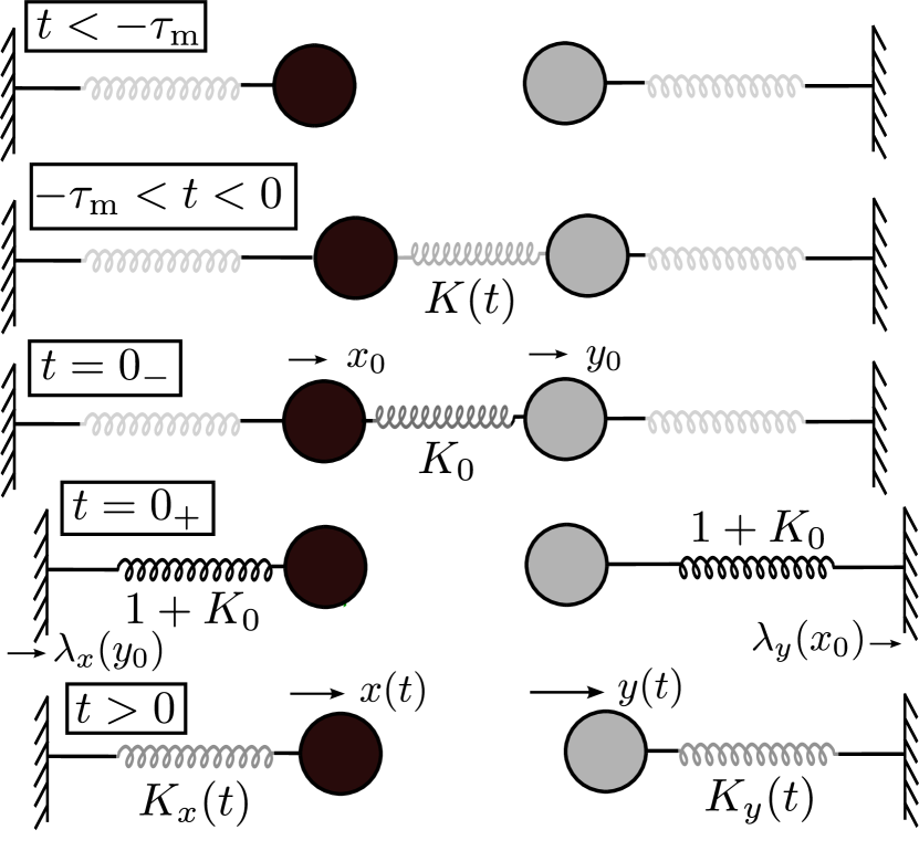
Figure 1: Two oscillators in a noisy environment are coupled and decoupled in the period $-\tau_{{\rm m}}\leq t\leq 0$ using a harmonic spring of strength $K(t)$. The spring strengths $K_{x,y}$ are adjusted and tether points $\lambda_{x,y}$ shifted, using feedback from the displacements $x_{0}$ and $y_{0}$ at $t=0$, in preparation for an exploitation procedure in the period $t>0$.

The pdf satisfying the Fokker-Planck equation in the measurement interval takes the form

$$\!p(x,y,t)\!=\!\frac{[1+2\tilde{K}]^{\frac{1}{2}}}{2\pi}\exp\!\left[-\frac{x^{2}}{2}-\frac{y^{2}}{2}-\frac{\tilde{K}(y-x)^{2}}{2}\right]\!,\!\!$$ (3)

with the time-dependent parameter $\tilde{K}(t)$ determined by

$$d\tilde{K}/dt=-2(\tilde{K}-K)(1+2\tilde{K}),$$ (4)

with $\tilde{K}(-\tau_{{\rm m}})=0$. In the quasistatic limit, $\tilde{K}(t)$ follows the evolution of the coupling strength $K(t)$ exactly. The stochastic entropy production during measurement is given by Seifert (2008); Spinney and Ford (2012); Ford (2016, 2013)

$$d\Delta s_{{\rm tot}}^{{\rm m}} = (\tilde{K}-K)\Bigl{[}4dt-(1+2\tilde{K})(y-x)^{2}dt$$ (5)

$$+(x-y)(dx-dy)\Bigr{]},$$

which implies a mean rate of production

$$d\langle\Delta s_{{\rm tot}}^{{\rm m}}\rangle/dt=4(\tilde{K}-K)^{2}/(1+2\tilde{K}).$$ (6)

At $t=0$, the joint pdf may be represented as $p(x_{0},y_{0},0)=p(x_{0},0|y_{0})p(y_{0},0)$ where $x_{0}=x(0)$ and $y_{0}=y(0)$, with the state of the first oscillator described by a conditional pdf

$$p(x_{0},0|y_{0}) = [(1+\tilde{K}_{0})/2\pi]^{1/2}$$ (7)

$$\times \exp\left[\!-\frac{(1+\tilde{K}_{0})}{2}\left(x_{0}-\frac{\tilde{K}_{0}y_{0}}{1+\tilde{K}_{0}}\right)^{2}\right],\quad$$

where $\tilde{K}_{0}=\tilde{K}(0)$, and the second oscillator described by

$$p(y_{0},0)=\left(\kappa/2\pi\right)^{1/2}\exp(-\kappa y_{0}^{2}/2),$$ (8)

with $\kappa=(1+2\tilde{K}_{0})/(1+\tilde{K}_{0})$.

If the measurement process took the form of quasistatic coupling and instantaneous decoupling (denoted ‘qi’), for which $\tilde{K}_{0}$ would equal $K_{0}$, the mean work of measurement would be a free energy of coupling minus the mean energy of the coupling spring at $t=0$, which is

$$\langle W_{{\rm m}}^{{\rm qi}}\rangle=\frac{1}{2}\ln(1+2K_{0})-\frac{K_{0}}{1+2K_{0}}.$$ (9)

In the third period $0\leq t\leq\tau_{{\rm e}}$ the outcome of the measurement is exploited through changes in the strengths $K_{x}(t)$ and $K_{y}(t)$ of the oscillator springs and the positions $\lambda_{x}$ and $\lambda_{y}$ of their tethering points. Optimal exploitation sequences for a single oscillator after measurement have been studied previously Abreu and Seifert (2011); Granger and Kantz (2011); Sagawa and Ueda (2012a). We similarly employ $\lambda_{x}=K_{0}y_{0}/(1+K_{0})$, $\lambda_{y}=K_{0}x_{0}/(1+K_{0})$, and $K_{x}(0)=K_{y}(0)=1+K_{0}$, the rationale for which will become clear, and $K_{x}(\tau_{{\rm e}})=K_{y}(\tau_{{\rm e}})=1$. The changes at the start of the ‘exploitation’ interval are indicated in Fig. 1 (labelled $t=0_{+}$). The subsequent dynamics are modelled using

$$dx = -K_{x}(t)(x-\lambda_{x})dt+\sqrt{2}\,dW_{x},$$

$$dy = -K_{y}(t)(y-\lambda_{y})dt+\sqrt{2}\,dW_{y},$$ (10)

and the work of exploitation is given by

$$W_{{\rm e}}=\int_{0}^{\tau_{{\rm m}}}\frac{1}{2}\left[\frac{dK_{x}}{dt}\left(x(t)-\lambda_{x}\right)^{2}+\frac{dK_{y}}{dt}\left(y(t)-\lambda_{y}\right)^{2}\right]dt.$$ (11)

If the pdf $p(x_{0},y_{0},0)$ is characterised by $\tilde{K}_{0}=K_{0}$ and if instantaneous changes to the spring strengths and tether points are followed by a quasistatic evolution of $K_{x}$ and $K_{y}$ (a process denoted ‘iq’), then the mean work of exploitation is given by

$$\langle W_{{\rm e}}^{{\rm iq}}\rangle=\frac{K_{0}}{2(1+2K_{0})}-\frac{1}{2}\ln(1+K_{0}),$$ (12)

for each oscillator. The mean work of measurement and exploitation for a protocol consisting of quasistatic coupling, instantaneous decoupling and changes in spring parameters, followed by further quasistatic processing (denoted ‘qiiq’) is therefore

$$\!\langle W_{{\rm m+e}}^{{\rm qiiq},1}\rangle=\langle W_{{\rm m}}^{{\rm qi}}\rangle+\langle W_{{\rm e}}^{{\rm iq}}\rangle=\!\frac{1}{2}\ln\!\left[\frac{1+2K_{0}}{1+K_{0}}\right]-\frac{K_{0}}{2(1+2K_{0})},$$ (13)

for exploitation of just the first oscillator (i.e. where $K_{y}$ and $\lambda_{y}$ are not modified for the exploitation interval). Since this mean work cannot be negative, the second law is preserved. However, if both oscillators are subjected to the exploitation procedure we get

$$\langle W_{{\rm m+e}}^{{\rm qiiq},2}\rangle=\langle W_{{\rm m}}^{{\rm qi}}\rangle+2\langle W_{{\rm e}}^{{\rm iq}}\rangle=\frac{1}{2}\ln\left[\frac{1+2K_{0}}{(1+K_{0})^{2}}\right]\leq 0,$$ (14)

which offers the prospect of a violation of the law.

To check such a claim, we compute the stochastic entropy production during exploitation. We write the pdf as $p(x,y,t)=p(x,t|y_{0})p(y,t|x_{0})$, such that at $t=0$ the conditional pdf $p(x,t|y_{0})$ takes the form in Eq. (7) and $p(y,t|x_{0})$ is given by Eq. (8). This asymmetric specification of the pdf provides a rationale for the chosen exploitation protocol. If a quasistatic-instantaneous (qi) measurement procedure has been performed, such that $\tilde{K}_{0}=K_{0}$, then the changes made to $K_{x}$ and $\lambda_{x}$ at $t=0$ effectively place the first oscillator in a state of canonical equilibrium. A subsequent quasistatic evolution of the spring strength of the first oscillator could be carried out without the generation of entropy.

In general, however, the evolving pdf of the first oscillator would be written

$$p(x,t|y_{0})\!=\![\tilde{K}_{x}(t)/2\pi]^{1/2}\exp(-\tilde{K}_{x}(t)[x-\bar{x}(t)]^{2}/2),\,\!\!\!$$ (15)

with time-dependent parameters $\tilde{K}_{x}(t)$ and $\bar{x}(t)$ given by

$$d\tilde{K}_{x}/dt = -2\tilde{K}_{x}(\tilde{K}_{x}-K_{x}),$$ (16)

$$d\bar{x}/dt = -K_{x}[\bar{x}-\lambda_{x}(y_{0})],$$ (17)

subject to $\tilde{K}_{x}(0)=1+\tilde{K}_{0}$ and $\bar{x}(0)=\tilde{K}_{0}y_{0}/(1+\tilde{K}_{0})$. The stochastic entropy production associated with the first oscillator during exploitation is Spinney and Ford (2012)

$$d\Delta s_{{\rm tot}}^{x}=(2-\tilde{K}_{x}[x-\bar{x}]^{2})(\tilde{K}_{x}-K_{x})dt+K_{x}\lambda_{x}dx$$

$$-\tilde{K}_{x}\bar{x}dx\!+\!\tilde{K}_{x}(x-\bar{x})K_{x}(\bar{x}-\lambda_{x})dt\!-\!(K_{x}-\tilde{K}_{x})xdx.\qquad$$ (18)

For a qi measurement process $\tilde{K}_{0}=K_{0}$ and $\bar{x}(0)=\lambda_{x}$, in which case $d\Delta s_{{\rm tot}}^{x}$ reduces to

$$\!d\Delta s_{{\rm tot}}^{{\rm qi},x}\!\!=\!(\tilde{K}_{x}-K_{x})(2dt-\tilde{K}_{x}[x-\lambda_{x}]^{2}dt+[x-\lambda_{x}]dx),$$ (19)

leading to an average rate of production

$$d\langle\Delta s_{{\rm tot}}^{{\rm qi},x}\rangle/dt=(\tilde{K}_{x}-K_{x})^{2}/\tilde{K}_{x}.$$ (20)

Similarly, the pdf of the second oscillator may be written

$$\!p(y,t|x_{0})=[\tilde{K}_{y}(t)/2\pi]^{1/2}\exp(-\tilde{K}_{y}(t)[y-\bar{y}(t)]^{2}/2),\!\!\!\!$$ (21)

for the exploitation interval, with

$$d\tilde{K}_{y}/dt = -2\tilde{K}_{y}(\tilde{K}_{y}-K_{y}),$$ (22)

$$d\bar{y}/dt = -K_{y}[\bar{y}-\lambda_{y}(x_{0})],$$ (23)

but this time subject to $\tilde{K}_{y}(0)=(1+2\tilde{K}_{0})/(1+\tilde{K}_{0})$ and $\bar{y}(0)=0$. The stochastic entropy production associated with the second oscillator during exploitation is Spinney and Ford (2012)

$$d\Delta s_{{\rm tot}}^{y}\!=\!(2-\tilde{K}_{y}[y-\bar{y}]^{2})(\tilde{K}_{y}-K_{y})dt\!+\!K_{y}\lambda_{y}dy$$

$$-\tilde{K}_{y}\bar{y}dy\!+\!\tilde{K}_{y}(y-\bar{y})K_{y}(\bar{y}-\lambda_{y})dt\!-\!(K_{y}-\tilde{K}_{y})ydy.\qquad$$ (24)

It is instructive to consider a special case where we assume $\tilde{K}_{0}=K_{0}$, set $K_{y}$ equal to $1+K_{0}$ for the initial part of the exploitation interval, and compute a stochastic entropy production $d\Delta s_{{\rm tot}}^{{\rm rel},y}$ associated with the relaxation of the parameters $\tilde{K}_{y}$ and $\bar{y}$ to $K_{y}$ and $\lambda_{y}(x_{0})$, respectively. This is the key to understanding the breakage of the second law. The mean rate of production, averaged over $x_{0}$ and $y_{0}$, is given by

$$d\langle\Delta s_{{\rm tot}}^{{\rm rel},y}\rangle/dt=-K_{0}^{2}\tilde{K}_{y}^{{\rm rel}}\exp[-2(1+K_{0})t]/(1+2K_{0}),$$ (25)

with $d\tilde{K}_{y}^{{\rm rel}}/dt=-2\tilde{K}_{y}^{{\rm rel}}(\tilde{K}_{y}^{{\rm rel}}-1-K_{0})$. Note that this mean rate of production is negative. After this relaxation, $d\langle\Delta s_{{\rm tot}}^{y}\rangle/dt$ takes the form of an analogue of Eq. (20) associated with the deviation between $\tilde{K}_{y}$ and $K_{y}$ over the remainder the exploitation interval.

In the final period $\tau_{{\rm e}}\leq t\leq\infty$ the oscillator spring constants have returned to unity and the system relaxes until there is no further stochastic entropy production. The shifts in the tether points are irrelevant to the irreversibility, since a quasistatic process can take the $\lambda_{x,y}$ back to zero at no cost in mean work or mean entropy production. This completes the cycle.

The only contribution to the mean total entropy production for a qiiq process involving exploitation of both oscillators is the relaxation represented by Eq. (25). When integrated over time this gives

$$\langle\Delta s_{{\rm tot}}^{{\rm rel},y}\rangle=\langle\Delta s_{{\rm tot}}^{{\rm qiiq},2}\rangle=\frac{1}{2}\ln\left[\frac{1+2K_{0}}{(1+K_{0})^{2}}\right]\leq 0,$$ (26)

which is consistent with the negative mean work $\langle W_{{\rm m+e}}^{{\rm qiiq},2}\rangle$ in Eq. (14) obtained from a cycle of measurement and exploitation under such conditions.

If exploitation is not invoked for the second oscillator, its relaxation would take place while $K_{y}$ remained equal to unity and with $\lambda_{y}=0$. The mean total entropy production for this case can be shown to be consistent with the positive mean work $\langle W_{{\rm m+e}}^{{\rm qiiq},1}\rangle$ in Eq. (13). Thus the mechanical and entropic assessments of irreversibility are consistent with one another for the special case of the qiiq process.

If the double demon oscillator system is processed slowly enough, we therefore expect environmental heat to be converted into stored potential energy, when averaged over many realisations, with a maximum change in the total thermodynamic entropy per cycle given by Eq. (26). This arises from the exploitation of each oscillator in a manner informed by the state of the other at $t=0$, a symmetrising of the feedback traditionally employed in a system-demon scenario. We next study how this might emerge in numerical simulations.

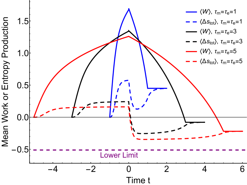
Figure 2: Evolution of the mean work performed on the two oscillator system (solid lines), and the associated mean stochastic entropy production (dashed lines), obtained from numerical simulations of the process specified in the main text, conducted over a range of timescales $\tau=\tau_{{\rm m}}=\tau_{{\rm e}}$. The quantities become equal when equilibrium is restored at the end of the process, and they approach a negative limit when the process timescale goes to infinity.

Equations (1) and (10) for the stochastic dynamics of the oscillators, (2) and (11) for the performance of work and (5), (18) and (24) for the production of stochastic entropy have been solved numerically for the following protocols of evolution of the spring constants: $K(t)=K_{0}(1+t/\tau_{{\rm m}})$ for $-\tau_{{\rm m}}\leq t\leq 0$, otherwise zero; $K_{x,y}(t)=(1+K_{0})-K_{0}t/\tau_{{\rm e}}$ for $0\leq t\leq\tau_{{\rm e}}$, otherwise unity; and tether positions $\lambda_{x}=K_{0}y_{0}/(1+K_{0})$ and $\lambda_{y}=K_{0}x_{0}/(1+K_{0})$ for $t\geq 0$, otherwise zero. Equations (4), (16), (17), (22) and (23) are solved in the appropriate time intervals to provide the necessary parameters $\tilde{K}(t)$, $\tilde{K}_{x}(t)$, $\bar{x}(t)$, $\tilde{K}_{y}(t)$, and $\bar{y}(t)$.

We choose $K_{0}=4$ and generate sets of realisations for various values of $\tau_{{\rm m}}$ and $\tau_{{\rm e}}$. The averages of work done and stochastic entropy produced are shown in Fig. 2 using a timestep of $5\times 10^{-4}$ and $10^{6}$ trajectories for each case. The two quantities coincide at the end of the cycle, as the laws of thermodynamics suggest they should, and for slower processes they approach the negative limit given by Eqs. (14) and (26). The reduction in entropy is achieved through the feedback invoked at $t=0$ and the partial harvesting of the potential energy of the springs. However, positive mean entropy production arises from the deviations of $\tilde{K}$, $\tilde{K}_{x}$ and $\tilde{K}_{y}$ from $K$, $K_{x}$ and $K_{y}$, respectively, and this occurs more strongly for faster processes.

We have shown that the stochastic evolution of two oscillators evolving according to a particular form of autonomous time-asymmetric dynamics can break the second law. Their interactions are conceived as an extension of a scenario where a measurement made by a device or demon is used to inform the exploitation of a system in order to convert environmental heat into work. In that case the second law is preserved because of a prior work of measurement, but passing feedback in both directions, thus allowing the device to be manipulated in a fashion informed by the system, extracts additional work. The total thermodynamic entropy can be reduced after completion of such a sequence of measurement and exploitation, and we attribute this to the self-sorting dynamics of the double demon.

We thank Stefan Grosskinsky and Rosemary J. Harris for helpful discussions, and acknowledge support from Engineering and Physical Sciences Research Council (EPSRC) Grant No. EP/I01358X/1, and the COST1209 network.

References

- Seifert (2008) U. Seifert, Eur. Phys. J. B 64, 423 (2008).
- Leff and Rex (2003) H. S. Leff and A. F. Rex, Maxwell’s Demon 2: Entropy, Classical and Quantum Information, Computing (Institute of Physics Publishing, 2003).
- Szilard (1929) L. Szilard, Z. f. Physik 53, 840 (1929).
- Maxwell (1871) J. C. Maxwell, Theory of Heat (Longmans, Green and Co., 1871).
- Earman and Norton (1998) J. Earman and J. D. Norton, Stud. Hist. Phil. Mod. Phys. 29, 435 (1998).
- Earman and Norton (1999) J. Earman and J. D. Norton, Stud. Hist. Phil. Mod. Phys. 30, 1 (1999).
- Hemmo and Shenker (2012) M. Hemmo and O. Shenker, The Road to Maxwell’s Demon (Cambridge, 2012).
- Brillouin (1951) L. Brillouin, J. Appl. Phys. 22, 334 (1951).
- Sagawa and Ueda (2009) T. Sagawa and M. Ueda, Phys. Rev. Lett. 102, 250602 (2009).
- Granger and Kantz (2011) L. Granger and H. Kantz, Phys. Rev. E 84, 061110 (2011).
- Mandal and Jarzynski (2012) D. Mandal and C. Jarzynski, Proc. Natl. Acad. Sci. USA 109, 11641 (2012).
- Sagawa and Ueda (2012a) T. Sagawa and M. Ueda, Phys. Rev. E 85, 021104 (2012a).
- Sagawa and Ueda (2012b) T. Sagawa and M. Ueda, Phys. Rev. Lett. 109, 180602 (2012b).
- Ford (2016) I. J. Ford, Contemp. Phys. (2016), 10.1080/ 00107514.2015.1121604.
- Landauer (1961) R. Landauer, IBM J. Res. Dev. 5, 183 (1961).
- Bennett (1973) C. H. Bennett, IBM J. Res. Dev. 17, 525 (1973).
- Bennett (1982) C. H. Bennett, Int. J. Theor. Phys. 21, 905 (1982).
- Plenio and Vitelli (2001) M. B. Plenio and V. Vitelli, Contemp. Phys. 42, 25 (2001).
- Abreu and Seifert (2011) D. Abreu and U. Seifert, Eur. Phys. Lett. 94, 10001 (2011).
- Barato and Seifert (2013) A. C. Barato and U. Seifert, Eur. Phys. Lett. 101, 60001 (2013).
- Spinney and Ford (2012) R. E. Spinney and I. J. Ford, Phys. Rev. E 85, 051113 (2012).
- Ford (2013) I. J. Ford, Statistical Physics: an entropic approach (Wiley, 2013).