Effect of group organization on the performance of cooperative processes

Abstract

Problem-solving competence at group level is influenced by the structure of the social networks and so it may shed light on the organization patterns of gregarious animals. Here we use an agent-based model to investigate whether the ubiquity of hierarchical networks in nature could be explained as the result of a selection pressure favoring problem-solving efficiency. The task of the agents is to find the global maxima of NK fitness landscapes and the agents cooperate by broadcasting messages informing on their fitness to the group. This information is then used to imitate, with a certain probability, the fittest agent in their influence networks. For rugged landscapes, we find that the modular organization of the hierarchical network with its high degree of clustering eases the escape from the local maxima, resulting in a superior performance as compared with the scale-free and the random networks. The optimal performance in a rugged landscape is achieved by letting the main hub to be only slightly more propense to imitate the other agents than vice versa. The performance is greatly harmed when the main hub carries out the search independently of the rest of the group as well as when it compulsively imitates the other agents.

I Introduction

There is little dispute over the claim that the collective structures built by termites, ants and slime molds are products of cooperative work performed by a myriad of organisms who, individually, are inept to conceive the greatness of the structures they build Marais_37 . Thinking of those collective structures as the organisms’ solutions to the problems that endanger their existence, it is natural to argue that competence in problem solving should be viewed as a candidate selection pressure for molding the organization of groups of social animals Bloom_01 ; Queller_09 .

Information flows between individuals via social contacts and, in the problem-solving context, the relevant process is imitative learning as expressed in this quote by Bloom “Imitative learning acts like a synapse, allowing information to leap the gap from one creature to another” which summarizes his view of those collective structures as global brains Bloom_01 . Evidences that cooperative work powered by social learning is an efficient process to solve difficult problems are offered by the variety of social learning based optimization heuristics, such as the particle swarm optimization algorithm Bonabeau_99 and the adaptive culture heuristic Kennedy_98 ; Fontanari_10 .

From the perspective of the computer science, there has been considerable progress on the understanding of the factors that make cooperative group work effective Clearwater_91 ; Clearwater_92 ; Page_07 , although, somewhat disturbingly, the most popular account of collective intelligence, the so-called wisdom of crowds, involves the suppression of cooperation since its success depends on the individuals making their guesses independently of each other Surowiecki_04 (see, however, King_12 ).

In this contribution we build on a recently proposed minimal model of distributed cooperative problem-solving systems based on imitative learning Fontanari_14 to study the influence of the social network topology on the performance of cooperative processes. Individuals cooperate by broadcasting messages informing on their fitness and use this information to imitate, with a certain probability, the fittest individual in their influence networks. The task of the individuals is to find the global maxima of smooth and rugged fitness landscapes generated by the NK model Kauffman_87 ; Kauffman_89 and the performance or efficiency of the group is measured by the number of trials required to find those maxima.

Our goal is to investigate whether the ubiquity of hierarchical networks Ravasz_03 , which are both modular and scale-free, could be explained as the result of a selection pressure favoring problem-solving efficiency. In fact, for rugged landscapes we find that the hierarchical network performs better than the scale-free and the random networks. The modular organization of the hierarchical network with its high degree of clustering facilitates the system to escape local maxima, despite the presence of a hub with very high connectivity (super-spreader) which, in general, may cause great harm to the system performance by broadcasting misleading information about the location of the global maxima Francisco_16 as happens in the case of the scale-free network. For smooth landscapes, the topology of the network has little influence on the performance of the imitative search.

In addition, we find that for the three network topologies considered here, namely, hierarchical, scale-free and random topologies, allowing the main hub (i.e., the node with the highest degree) to explore the landscape without much consideration for the other individuals, even though those individuals may learn from it, is always detrimental to the performance of the system. Interestingly, for the hierarchical and scale-free networks, the optimal performance in a rugged landscape is achieved by letting the main hub to be only slightly more propense to imitate the other agents than vice versa. A compulsive imitator located at the main hub of the hierarchical network (or at the two main hubs of a scale-free network) leads to a disastrous performance. For the random network, where the main hub is not very influential, the performance is maximized by the compulsive imitation strategy. This is also true for the three topologies in the case of a smooth landscape, but the reason is that in the absence of local maxima it is always better to imitate the fittest individual in the group.

The rest of this paper is organized as follows. For the sake of completeness, we present a brief description of the NK model of rugged fitness landscapes in Section II. The rules of the agent-based model that implements the imitative search are explained in Section III and the three network topologies – hierarchical, scale-free and random – are presented in Section IV. In Section V we present and discuss the results of the simulations of the imitative search on rugged and smooth NK landscapes for those three topologies. Finally, Section VI is reserved to our concluding remarks.

II NK Model of Rugged Fitness Landscapes

The NK model is a computational framework to generate families of statistically identical rugged fitness landscapes. It was proposed by Stuart Kauffman in the late 1980s aiming at modeling evolution as an incremental process, the so-called adaptive walk, on rugged landscapes Kauffman_87 ; Kauffman_89 . Today the NK model is the paradigm of problem spaces with many local optima, being particularly popular among the organizational and management research community Levinthal_97 ; Lazer_07 ; Fontanari_16 .

The NK model is named for the two integer parameters that are used to randomly generate landscapes, namely, $N$ and $K$. The landscape is defined in the space of binary strings of length $N$ and so this parameter determines the size of the solution space, $2^{N}$. The other parameter $K=0,\ldots,N-1$ influences the ruggedness of the landscape. In particular, the correlation between the fitness of any two neighboring strings (i.e., strings that differ at a single component) is $1-\left(K+1\right)/N$ Kauffman_89 . Hence $K=0$ corresponds to a smooth landscape whereas $K=N-1$ corresponds to a completely uncorrelated landscape. For concreteness, next we describe briefly the procedure to generate a random realization of a NK landscape.

The $2^{N}$ distinct binary strings of length $N$ are denoted by $\mathbf{x}=\left(x_{1},x_{2},\ldots,x_{N}\right)$ with $x_{i}=0,1$. To each string $\mathbf{x}$ we associate a fitness value $\Phi\left(\mathbf{x}\right)$ which is an average of the contributions from each component $i$ in the string, i.e., $\Phi\left(\mathbf{x}\right)=\sum_{i=1}^{N}\phi_{i}\left(\mathbf{x}\right)/N$, where $\phi_{i}$ is the contribution of component $i$ to the fitness of string $\mathbf{x}$. It is assumed that $\phi_{i}$ depends on the state $x_{i}$ as well as on the states of the $K$ right neighbors of $i$, i.e., $\phi_{i}=\phi_{i}\left(x_{i},x_{i+1},\ldots,x_{i+K}\right)$ with the arithmetic in the subscripts done modulo $N$. The functions $\phi_{i}$ are $N$ distinct real-valued functions on $\left\{0,1\right\}^{K+1}$ but the usual procedure is to assign to each $\phi_{i}$ a uniformly distributed random number in the unit interval Kauffman_89 , which then guarantees that $\Phi\in\left(0,1\right)$ has a unique global maximum.

For $K=0$ the global maximum is the sole maximum of $\Phi$, which can be easily found by picking for each component $i$ the state $x_{i}=0$ if $\phi_{i}\left(0\right)>\phi_{i}\left(1\right)$ or the state $x_{i}=1$, otherwise. For $K=N-1$, the (uncorrelated) landscape has on the average $2^{N}/\left(N+1\right)$ maxima with respect to single bit flips Derrida_81 . Finding the global maximum of the NK model for $K>0$ is a NP-complete problem Solow_00 , which means that the time required to solve the problem using any currently known deterministic algorithm increases exponentially fast with the length $N$ of the strings Garey_79 .

We note that the specific features of a realization of the NK landscape (e.g., number and location of the local maxima with respect to the global maximum) are not fixed by the parameters $N$ and $K$, because the components $\phi_{i}$ are chosen randomly in the unit interval. This is the reason that finding the global maximum for any realization of the NK landscape for large $N$ and $K>0$ is an extremely difficult computational problem Solow_00 . Hence, in order to better apprehend the influence of the network topology and, in particular, the role of the main hub on the performance of cooperative problem-solving systems, here we use a single realization of the NK fitness landscape for fixed values of $N$ and $K$.

More pointedly, we consider two types of landscape: a smooth landscape with $N=16$ and $K=0$ and a rugged landscape with $N=16$ and $K=5$. Since for $K=0$ all NK landscapes are equivalent, there is no lack of generality in considering a single instance of that family. The particular realization of the NK landscape with $N=16$ and $K=5$ considered here exhibits 296 maxima in total, among which 295 are local maxima. The mean relative fitness of the local maxima with respect to the fitness of the global maximum is $0.81$ whereas the mean relative fitness of all strings is $0.60$. It is interesting to note that for large $N$ the NK model exhibits the so-called complexity catastrophe Kauffman_89 , i.e., as $N$ increases the fitness of the local maxima become poorer to such a point that they are not better than the fitness of a randomly chosen string. The effects of averaging over different realizations of the rugged landscape is addressed briefly at the end of Section V.

III Imitative learning search

We consider a system composed of $L$ agents $i=1,\ldots,L$ and assume that each agent operates in an initial binary string drawn at random with equal probability for the bits $0$ and $1$. Agent $i$ can choose between two distinct processes to operate on its string. The first process, which happens with probability $1-p_{i}$, is the elementary move in the solution space that consists of picking a bit at random from the string and flipping it. This elementary move allows the agents to explore in an incremental way the entire solution space formed by the $2^{N}$ binary strings. The second process, which happens with probability $p_{i}$, is the imitation of a model string. Here the model string is defined as the string that exhibits the largest fitness value among the (fixed) subgroup of agents that can influence (i.e., are connected to) agent $i$. The model string and the string $i$ (i.e., the string operated by agent $i$) are compared and the different bits are singled out. Then agent $i$ selects at random one of the distinct bits and flips it so that this bit is now the same in both string $i$ and the model string. After imitation these two strings become more similar, as expected. In the case the string $i$ is identical to the model string, agent $i$ executes the elementary move with probability one.

The parameter $p_{i}\in\left[0,1\right]$ is the imitation propensity of agent $i$. The case $p_{i}=0$ corresponds to the baseline situation in which agent $i$ explores the solution space independently of the other agents. The imitation procedure described above was based on the incremental assimilation mechanism used to study the influence of an external media Shibanai _01 ; Peres_11 in the celebrated Axelrod’s model of culture dissemination Axelrod_97 . We note that an alternative non-incremental imitation procedure, which allows string $i$ to become identical to the model string by changing many bits simultaneously, may permanently stuck the search in the local maxima Lazer_07 .

The evolution of the system of $L$ agents proceeds as follows. At each time $t$ we pick an agent at random, say agent $i$, and allow it to operate on its associated string either by imitating the model string or by flipping a bit at random. Since this operation always results in a change of fitness of string $i$, which may become larger than the fitness of the model string, we need to update the model string status at each time. As usual in such asynchronous update scheme, we choose the time unit as $\Delta t=1/L$ so that during the increment from $t$ to $t+1$, exactly $L$ string operations are performed, though not necessarily by $L$ distinct agents.

The search ends when one of the agents finds the global maximum and we denote by $t^{*}$ the halting time. The efficiency of the search is defined as the total number of string operations necessary to find the global maximum (i.e., $Lt^{*}$) and so the computational cost of the search can be defined as $C\equiv Lt^{*}/2^{N}$, where for convenience we have rescaled $t^{*}$ by the size of the solution space $2^{N}$.

In the case of the independent search (i.e., $p_{i}=0,\forall i$) the ruggedness of the landscape has no effect on the efficiency of the search, which depends only on the length of the strings, $N$ and on the system size $L$. It can be shown that the mean computational cost is given by Fontanari_15

$$\langle C\rangle=\frac{L}{2^{N}\left[1-\left(\lambda_{N}\right)^{L}\right]},$$ (1)

where $\lambda_{N}$ is the second largest eigenvalue of a tridiagonal stochastic matrix $\mathbf{T}$ with elements $T_{ij}=\left(1-j/N\right)\delta_{i,j+1}+j/N\delta_{i,j-1}$ for $j=1,\ldots,N-1$, $T_{i0}=\delta_{i,1}$, and $T_{iN}=\delta_{i,N}$. Note that $i=N$ is the only absorbing state of the stochastic process defined by $\mathbf{T}$. Here $\delta_{i,j}$ is the Kronecker delta and the notation $\langle\ldots\rangle$ stands for the average over independent searches on the same landscape. In particular, for $N=16$ we find $\lambda_{16}\approx 0.9999859$ and since $\left(\lambda_{16}\right)^{L}\approx e^{-L\left(1-\lambda_{16}\right)}$ we have $\langle C\rangle\approx 1.08$ for $L\ll 1/\left(1-\lambda_{16}\right)\approx 70740$ and $\langle C\rangle\approx L/2^{16}$ for $L\gg 70740$. The first regime, characterized by a mean computational cost that is independent of the system size $L$, corresponds to the situation where the halting time $t^{*}$ decreases linearly with increasing $L$. The second regime, where $\langle C\rangle$ increases linearly with $L$, corresponds to the situation where the halting time is $t^{*}\approx 1$, i.e., the system size is so large that the global maximum is likely to be found already during the initial stage when the strings are generated randomly.

IV Complex networks

Most real-world social networks are scale-free and exhibit a high degree of clustering, which seems to be independent of the number of nodes $L$ Albert_02 . The scale-free property means that the probability that a randomly selected node has degree $k$ obeys a power law $P\left(k\right)\sim k^{-\gamma}$ where the degree exponent $\gamma$ usually varies between $1$ and $3$. The high degree of clustering is consequence of the formation of cliques, which represent groups of individuals in which every member knows every other member. Typical scale-free networks produced by the Barabási-Albert algorithm and by its many variants Barabasi_99 do not exhibit a high degree of clustering and therefore do not account for the presence of both properties of real networks. The reason seems to be the absence of a modular organization in scale-free networks Ravasz_03 . To produce a network that exhibits both modularity (hence, a high degree of clustering) and the scale-free topology it is necessary to organize the modules hierarchically, producing the so-called hierarchical network Ravasz_03 .

We note, for the sake of completeness, that the clustering coefficient for a node $i$ with $k_{i}$ links is defined as ${\mathcal{C}}_{i}=2n_{i}/\left[k_{i}\left(k_{i}-1\right)\right]$, where $n_{i}$ is the number of links between the $k_{i}$ neighbors of node $i$, and the overall level of clustering in a network can be obtained by averaging those coefficients over all nodes, $\bar{\mathcal{C}}=\sum_{i}^{L}{\mathcal{C}}_{i}/L$ Watts_98 .

Here we consider three types of networks, which share the same number of nodes and links, but exhibit very different topologies, as reflected by their degree distributions and their average clustering coefficients. In particular, we consider hierarchical networks, scale-free networks and random networks. In what follows we describe succinctly each of these networks.

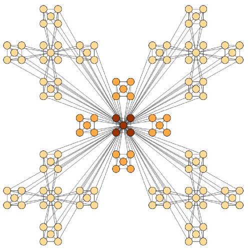
Figure 1: (Color online) Hierarchical network with $L=125$ nodes and $394$ links, where each elementary cluster of five nodes is fully connected (the links connecting the diagonal nodes in the elementary clusters are not visible). The central node of the original cluster at level $1$ has degree $k=84$ and the four central nodes at level $3$ have degree $k=20$. The other nodes have degrees $k=4,5$ and $6$. The mean clustering coefficient is $\bar{\mathcal{C}}=0.850$.

IV.1 Hierarchical network model

The starting point of the procedure to construct a hierarchical network that is both modular and scale-free Ravasz_03 is a cluster of five fully connected nodes, arranged in the corners and in the center of a square. This is level $1$ of the hierarchical network. Next, four replicas of this square are generated and the nodes at the corners of those replicas are linked to the central node, resulting in level $2$ of the hierarchy, composed of 20 nodes. Level $3$ is formed by generating four replicas of this 25 nodes module (i.e., the combination of levels $1$ and $2$) and linking the 16 peripheral nodes of each replica to the central node of the old module. Levels $1$, $2$ and $3$ form a new module with 125 nodes. The next step (level $4$) would be to produce again four replicas of this module and connect the peripheral sites to the central node of the old module. If a hierarchical network has $n$ levels then the total number of nodes is $L=5^{n}$ and the total number of links is $6\left(5^{n-1}\right)+4\left(5^{n}-4^{n}\right)$. Figure 1 illustrates the hierarchical network with $n=3$ levels. There are 40 nodes that exhibit the maximum value of the clustering coefficient, i.e. ${\mathcal{C}}_{i}=1$ and the main hub at the center of the original module is the node that exhibits the lowest value of this coefficient, ${\mathcal{C}}_{i}\approx 0.036$.

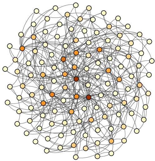
Figure 2: (Color online) Realization of a scale-free network with $L=125$ nodes and $394$ links generated using preferential attachment and network growth following the Barabási-Albert algorithm Barabasi_99 . The highest degree is $k=32$ (2 nodes) and the lowest is $k=3$ (45 nodes). The mean clustering coefficient is $\bar{\mathcal{C}}=0.180$.

IV.2 Scale-free network

A scale-free network is a network whose degree distribution follows a power law when the number of nodes $L$ is very large Albert_02 , and so the network may exhibit a few nodes with very large degrees. As already pointed out, the interesting feature of this topology is that, while exhibiting the scale-free property, it lacks modularity which allows us then to examine the influence of this property on the performance of distributed cooperative problem-solving systems. In order to generate scale-free networks with a fixed number of nodes (say, 125 nodes) and links (say, 394 links) we have made a minor change in the classical Barabási-Albert algorithm Barabasi_99 . As it is well-known, this algorithm is based on a preferential attachment mechanism and network growth. Beginning with $m_{0}$ disconnected nodes, at each time step, a new node $i$ with $m_{0}$ links is added to the network. The probability that a node $j$, which is present in the network, will receive a link from $i$ is proportional to the degree of node $j$, i.e., $P(i\to j)=k_{j}/\sum_{l}k_{l}$.

To generate a scale-free network with a fixed number of nodes and links, we use the following procedure. Given the desired ratio $r^{*}$ between the number of links and the number of nodes, which in the case of interest is $r^{*}=394/125=3.152$, we begin the network growing procedure at generation $\tau=0$ with $m_{0}=\lceil r^{*}\rceil=4$ disconnected nodes, so that the ratio at this initial stage is $r_{0}=0/4=0$. Since $r_{0}<r^{*}$, we add a new node with $m_{0}$ links to the original nodes so that at generation $\tau=1$ we have $r_{1}=4/5$. We keep doing this till growing generation $\tau=15$ at which $r_{15}=60/19>r^{*}$, when we add then a new node with $m_{0}-1=3$ links, yielding $r_{16}=63/20<r^{*}$ at generation $\tau=16$. The next node which will form generation $\tau=17$ will have then $m_{0}$ links. The idea is that if at growing generation $\tau-1$ we have $r_{\tau-1}<r^{*}$ the new node at generation $\tau$ will have $m_{0}$ links, otherwise it will have $m_{0}-1$ links. The network is complete when the number of nodes reaches the desired value, $L=125$ in our case. In Fig. 2 we exhibit a realization of a scale-free network produced by the procedure just described. There are $32$ nodes with ${\mathcal{C}}_{i}=0$, (i.e., there are no links between the nodes that are linked to node $i$) and the highest clustering coefficient is ${\mathcal{C}}_{i}=0.67$.

IV.3 Random network

The random network offers a good baseline for comparison with the two structured networks described before. In this case we simply distribute randomly and without replacement the fixed number of links (say, 394) among the $L\left(L-1\right)/2$ pairs of nodes. Figure 3 exhibits a realization of a random network. There are $50$ nodes with ${\mathcal{C}}_{i}=0$ and the highest clustering coefficient is ${\mathcal{C}}_{i}=0.33$.

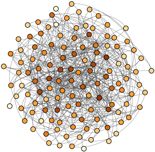
Figure 3: (Color online) Realization of a random network with $L=125$ nodes and $394$ links. The highest degree is $k=12$ (2 nodes) and the lowest is $k=1$ (4 nodes). The mean clustering coefficient is $\bar{\mathcal{C}}=0.057$.

Finally, we note that while the procedure to construct the hierarchical network is deterministic (i.e., the resulting network is unique), the procedures to generate the scale-free and the random networks are stochastic and so each time those procedures are implemented a different network is produced. Figures 2 and 3 then illustrate typical realizations of those two network topologies.

V Results

We begin this section with the analysis of the performance of the imitative search on a rugged NK landscape with parameters $N=16$ and $K=5$ (see Section II). To better appreciate the effects of the local maxima on the performance of the search we conclude the section with the analysis of a smooth landscape with parameters $N=16$ and $K=0$. Although the topology of the networks connecting those agents is variable (i.e., hierarchical, scale-free and random), the average connectivity of the networks as well as the number of nodes are fixed. The mean computational cost is calculated by averaging the computational cost over $10^{5}$ distinct searches. For the scale-free and the random networks, for each of those searches we generate a different network. In all figures exhibited in this section, the error bars are smaller than the symbol sizes.

V.1 Rugged Landscape

Figure 4 shows the mean computational cost for the hierarchical, small-world and random networks in the case that all agents have the same imitation propensity $p$. We find that $\langle C\rangle$ is quite insensitive to variations on the topology of the network for small values of $p$. In particular, for $p=0$ one recovers the results of the independent search, $\langle C\rangle\approx 1.08$, regardless of the topology. The topology becomes relevant only when the imitation propensity is large enough (say, $p>0.55$) to allow the model string to drive the system towards the local maxima and, in this case, the sensitivity to the topology is extreme. This figure reveals that for large $p$ the system can easily be trapped by the local maxima, from which escape can be extremely costly. This is akin to the groupthink phenomenon Janis_82 , when everyone in a group starts thinking alike, which can occur when people put unlimited faith in a talented leader (the model strings, in our case). A similar maladaptive behavior induced by imitation (or, more generally, social learning) has been observed in groups of guppies Laland_98 ; Laland_11 .

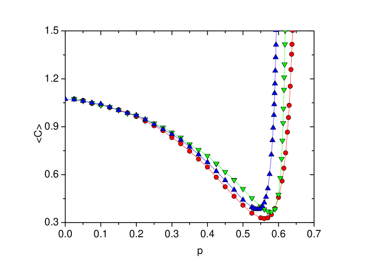
Figure 4: (Color online) Mean computational cost $\langle C\rangle$ as function of the imitation probability $p$ for the hierarchical network illustrated in Fig. 1 $(\CIRCLE)$, the scale-free network $(\blacktriangle)$, and the random network $(\blacktriangledown)$. The number of nodes is $L=125$ and the total number of links is $394$ for the three topologies. The parameters of the rugged NK landscape are $N=16$ and $K=5$.

Most remarkably, Fig.  4 reveals that the hierarchical network consistently outperforms the other two topologies regardless of the value of the imitation propensity of the agents. It is expected that the presence of large hubs (or super-spreaders) will enhance the performance of the system provided the information they broadcast is accurate Francisco_16 . This is not the case when the model string and its followers are stuck in the neighborhood of a local maxima and this is the reason that the random network performs better than the scale-free network for $p>0.55$. Although the hierarchical network exhibits a super-spreader with a degree much larger than the hubs of the scale-free network (see Figs. 1 and 2), its modular structure somehow slows down the spreading of the inaccurate information through the system.

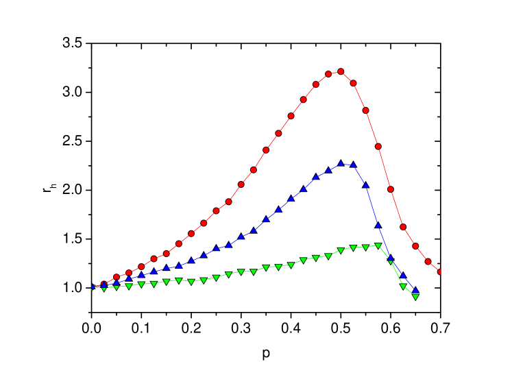
Figure 5: (Color online) Ratio $r_{h}$ between the probability $P_{h}$ that the agent with the highest degree in the network finds the global maximum and the baseline probability $1/L$ for the case the $L$ agents are equiprobable to find that maximum. The symbols $(\CIRCLE)$ are the results for the hierarchical network, $(\blacktriangle)$ are for the scale-free network, and $(\blacktriangledown)$ are for the random network $(\blacktriangledown)$. The number of nodes is $L=125$ and the total number of links is $394$ for the three network topologies. The parameters of the rugged NK landscape are $N=16$ and $K=5$.

It is instructive to examine whether the degree of a node has any influence on the chances that the node finds the global maximum of the NK landscape. To investigate this issue we evaluate the probability $P_{h}$ that the agent with the highest degree (main hub) is the one that finds the global maximum. Since in the case all agents have the same probability of finding the global maximum this probability is $1/L$, it is convenient to consider the ratio $r_{h}=P_{h}/\left(1/L\right)=LP_{h}$ which gives a measure of the odds of the main hub to find the solution relative to a situation where all agents are equiprobable to find the solution. Such equalitarian situation occurs most notably in the independent search (i.e., $p_{i}=0,\forall i$) or in a regular lattice where all nodes have the same degree and imitation propensity. In Fig. 5 we show $r_{h}$ as function of the imitation propensity $p$. The results are qualitatively the same for the three topologies under examination: for small $p$ the degree of a node is of little relevance, as expected, and as $p$ increases and reaches the optimal value at which the computational cost is minimum (see Fig. 4), the importance of the degree of the node on its chances of finding the solution (and the consequent boosting of the overall performance of the system) is greatly amplified. For large $p$, however, the main hub seems to play a very detrimental role on the system performance. In fact, its meager chances of finding the solution indicates that it is typically trapped in a local maximum and, due to its large influence on the other agents, has dragged them together.

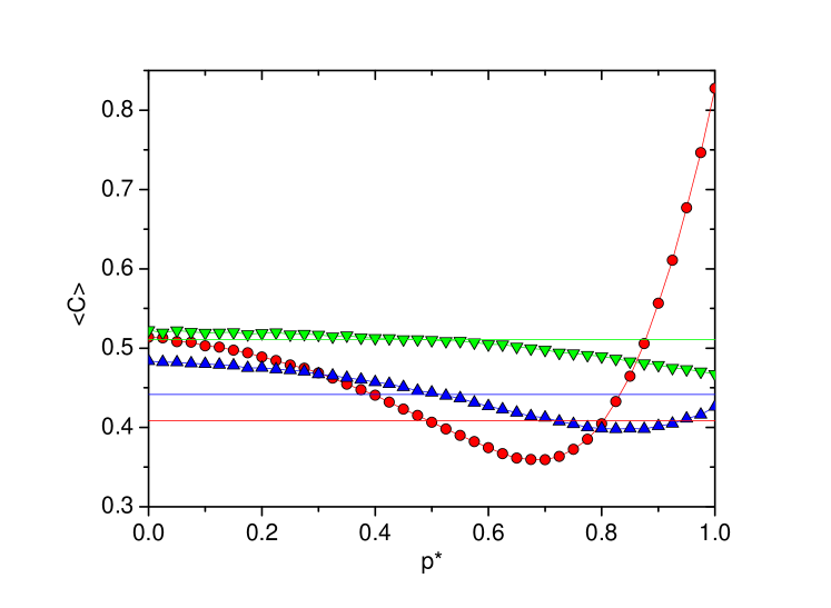
Figure 6: (Color online) Mean computational cost $\langle C\rangle$ as function of the imitation propensity $p^{*}$ of the agent with the highest degree for the hierarchical network $(\CIRCLE)$, the scale-free network $(\blacktriangle)$, and the random network $(\blacktriangledown)$. All other agents have their imitation propensities set to $p=0.5$. The horizontal lines indicate the computational costs for $p^{*}=p=0.5$. The number of nodes is $L=125$ and the total number of links is $394$ for the three network topologies. The parameters of the rugged NK landscape are $N=16$ and $K=5$.

Our next experiment consists of picking the node with the highest degree and setting its imitation propensity to the value $p^{*}$. The imitation propensities of the other $L-1$ agents in the system are assigned the same value $p$. In the case there are two or more nodes with the highest degree, we assign the distinctive imitation propensity value to only one of them. In this way we can examine the effect of disrupting the main hub of the network on the problem-solving efficiency of the system . The results for the three topologies are summarized in Fig. 6 for $p=0.5$

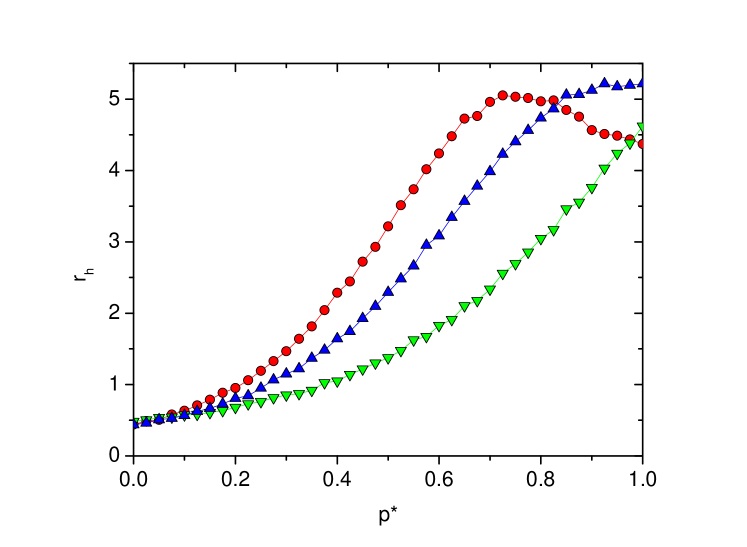
Figure 7: (Color online) Ratio $r_{h}$ between the probability $P_{h}$ that the agent with the highest degree in the network, which has imitation propensity $p^{*}$, finds the global maximum and the baseline probability $1/L$ for the case the $L$ agents are equiprobable to find that maximum. All other agents have imitation propensity set to $p=0.5$. The symbols $(\CIRCLE)$ are the results for the hierarchical network, $(\blacktriangle)$ are for the scale-free network, and $(\blacktriangledown)$ are for the random network $(\blacktriangledown)$. The parameters of the rugged NK landscape are $N=16$ and $K=5$.

As expected, the random network is the topology less sensitive to perturbations in a hub, because its hubs have degrees that are not significantly larger than the degree of a typical node. It is interesting that whereas the performance of the random network is unaffected for $p^{*}<p=0.5$, it shows a slight improvement for $p^{*}>p=0.5$, which means that the presence of a compulsive imitator in the group can be advantageous, provided its influence on the rest of the group is limited. As for the more structured networks, decreasing the imitation propensity of a hub relative to the rest of the group always results in a decrease of performance, whereas a moderate increase of the hub’s relative imitation propensity can be highly beneficial, though compulsive imitation can lead to a disastrous performance. These effects are much more pronounced in the hierarchical topology because of the very high degree of its main hub. In fact, when the second highest degree node is perturbed as well, the scale-free network exhibits a performance degradation for large $p^{*}$ similar to that observed for the hierarchical network (data not shown).

We note that the computational cost is minimized for $p^{*}>p$ (see Fig. 6), which suggests that variability in the imitation propensities of the agents may improve the performance of the cooperative system. This finding does not conflict with the claim that in a fully connected network the optimal performance is achieved by a homogeneous system Fontanari_16 because in the present analysis the agents differ in their degrees and so the situation $p=p^{*}$ does not correspond to a strictly homogeneous system.

Figure 7 shows the (relative) probability that the node with the highest degree finds the solution in comparison with the equiprobable scenario for the experiment summarized in Fig. 6. Since for $p^{*}\approx 0$ the main hub executes an independent search, its chances of finding the global maximum are meager as it does not benefit from the experience of the other agents, as expected. Note, however, that the agents connected to that hub may imitate it with probability $p=0.5$, in case it happens to become the model string of their influence networks. The odds the main hub hits the solution increases monotonically with increasing $p^{*}$, except for the hierarchical topology for which $r_{h}$ reaches a maximum exactly at the value of $p^{*}$ that minimizes the computational cost (see Fig. 6). The subsequent decrease of $r_{h}$ with increasing $p^{*}$ for $p^{*}\approx 1$ (compulsive imitation) as well as the disastrous performance of the system in this regime, highlight the nontrivial tradeoff between centrality and imitation propensity in the hierarchical network.

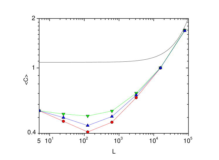
Figure 8: (Color online) Mean computational cost $\langle C\rangle$ as function of the number of sites $L$ for the hierarchical network $(\CIRCLE)$, the scale-free network $(\blacktriangle)$, and the random network $(\blacktriangledown)$. The imitation propensity is $p=0.5$ for all agents. The solid curve is the result for the independent search given by Eq. (1). The parameters of the rugged NK landscape are $N=16$ and $K=5$.

Finally, to conclude the analysis of the performance of the imitative search on a rugged landscape we address briefly two issues, namely, the effects of changing the system size $L$ and the realization of the landscape. In Fig. 8 we show the computational cost as function of the system size for the three network topologies and for the case that all agents have the same imitation propensity $p=0.5$. The total number of links is the same for all networks and it is determined by the number of links of the hierarchical network, namely, $6\left(5^{n-1}\right)+4\left(5^{n}-4^{n}\right)$ where $n=\ln L/\ln 5$. This implies that for $L=5$ the network is fully connected (i.e., it has 10 links), regardless of the topology. As observed in previous analyses of the imitative search Fontanari_14 ; Fontanari_15 , for the three topologies there is a system size at which the computational cost is minimum. Provided that the efficiency in solving problems has a selection value to the group members, this finding may offer an alternative explanation for the size of groups of gregarious animals, in addition to the more traditional selection pressures such as defense against predation, foraging success and the managing of the social relationships Wilson_75 ; Kurvers_14 ; Dunbar_92 . We note that, again, the hierarchical network outperforms the other two topologies, indicating that the combination of the modularity and the scale-free properties produces a very efficient organization for distributed cooperative problem-solving systems.

To check the influence of the specific realization of the NK rugged fitness landscape we used in our study, we have considered several random realizations of the landscape with $N=16$ and $K=5$. In Fig. 9 we show the results for the original realization (see Fig. 4) and for a particular realization that produced a very different quantitative outcome. These quantitative differences are due to variations in the number of local maxima for the different landscape realizations. We find that, despite the quantitative differences, the dependence of the computational cost on the imitation propensity is the same for all landscape realizations (not only for the two realizations shown in the figure), namely, an initial decrease towards an optimal value of $p$, followed by a steep increase due to the trapping in the local maxima. More importantly, the relative performances of the three topologies in the regime where the effect of the local maxima is critical are not altered by the landscape realization. In particular, the hierarchical network outperforms the other two topologies for all the realizations that we have generated.

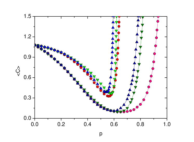
Figure 9: (Color online) Mean computational cost $\langle C\rangle$ as function of the imitation propensity $p$ for two realizations (the two bundles of data) of the NK fitness landscape with $N=16$ and $K=5$. The symbols $(\CIRCLE)$ are the results for the hierarchical network, $(\blacktriangle)$ are for the scale-free network, and $(\blacktriangledown)$ are for the random network.

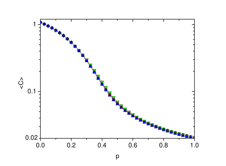
Figure 10: (Color online) Mean computational cost $\langle C\rangle$ as function of the imitation propensity $p$ for the hierarchical network illustrated in Fig. 1 $(\CIRCLE)$, the scale-free network $(\blacktriangle)$, and the random network $(\blacktriangledown)$. The number of nodes is $L=125$ and the total number of links is $394$ for the three network topologies. The parameters of the smooth NK landscape are $N=16$ and $K=0$.

V.2 Smooth landscape

We turn now to the analysis of the performance of the imitative search on a smooth landscape with $N=16$ and $K=0$. We note that for smooth landscapes ($K=0$) all landscape realizations are equivalent. Figure 10 shows that in the absence of local maxima the performances of the three topologies in the case $p_{i}=p,\forall i$ are practically indistinguishable in the scale of the figure and that the mean computational cost is a decreasing function of $p$, i.e., the best performance is attained by always imitating the model string ($p=1$) and allowing only their clones to explore the landscape through the elementary move. Figure 11 shows the (relative) odds that the main hub finds the maximum of the smooth landscape. There is a strong correlation between the degree of a node and its chances of finding the maximum. The saturation of $r_{h}$ with increasing $p>0.5$ indicates that system has lost diversity – all strings are clones or close neighbors of the model string – and so the odds of finding the solution is solely determined by the degree of the node.

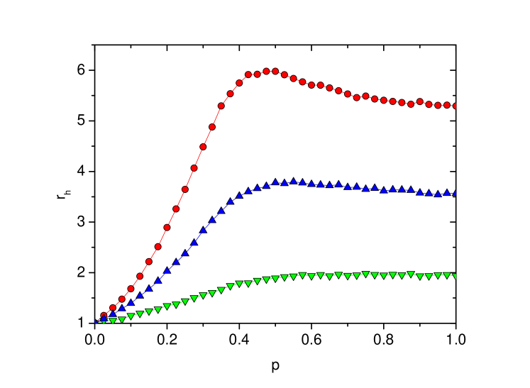
Figure 11: (Color online) Ratio $r_{h}$ between the probability $P_{h}$ that the agent with the highest degree in the network finds the global maximum and the baseline probability $1/L$ for the case the $L$ agents are equiprobable to find that maximum. The symbols $(\CIRCLE)$ are the results for the hierarchical network, $(\blacktriangle)$ are for the scale-free network, and $(\blacktriangledown)$ are for the random network $(\blacktriangledown)$. The number of nodes is $L=125$ and the total number of links is $394$ for the three network topologies. The parameters of the smooth NK landscape are $N=16$ and $K=0$.

Although the performances of the three topologies are very similar when all agents exhibit the same imitation propensities (see Fig. 10), the situation changes remarkably when the main hub is assigned the differential imitation propensity $p^{*}$ as shown in Fig. 12. Actually, in the scale of this figure we can observe that those performances in the case $p^{*}=p=0.5$ are not identical and that the scale-free network outperforms slightly the other two topologies. As in the case of the rugged landscape (see Fig. 6), the performance of the random network is affected little by making its main hub explore the landscape independently of the other agents. The performance of the hierarchical network, however, is extremely sensitive to the influence of its main hub. For the smooth landscape, the monotone decreasing of the computational cost with increasing $p^{*}$ for all topologies is simply a consequence of the fact that copying the fittest string at the trial is always a certain step towards the solution of the problem. This explains also the finding that the chances that the main hub finds the maximum is a steep increasing function of $p^{*}$ (data not shown).

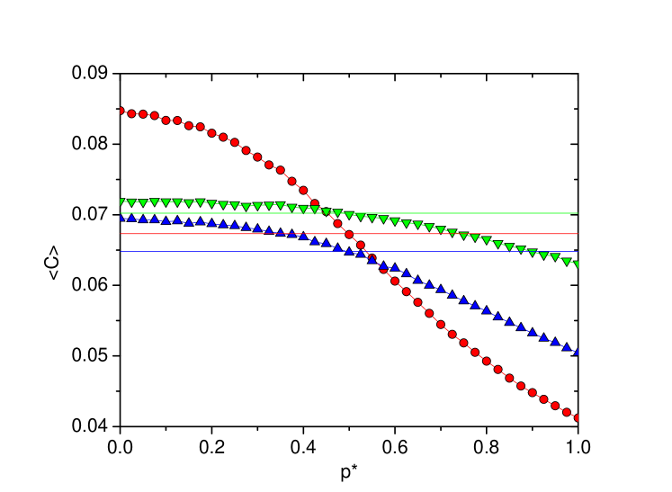
Figure 12: (Color online) Mean computational cost $\langle C\rangle$ as function of the imitation probability $p^{*}$ of the agent with the highest degree for the hierarchical network $(\CIRCLE)$, the scale-free network $(\blacktriangle)$, and the random network $(\blacktriangledown)$. All other agents have imitation propensity set to $p=0.5$. The horizontal lines indicate the computational costs of the homogeneous system $p^{*}=p=0.5$. The number of nodes is $L=125$ and the total number of links is $394$ for the three network topologies. The parameters of the smooth NK landscape are $N=16$ and $K=0$.

VI Discussion

Modularity is ubiquitous among biological entities, particularly among processes and structures that can be modelled as networks Carroll_01 ; Lipson_07 ; Wagner_07 . A network is said to be modular if it exhibits highly connected clusters of nodes that are scantily connected to nodes in other clusters. Modular systems are more adaptable since they are much easier to rewire and be co-opted for another functions than monolithic networks. In addition, modular systems minimize the cost of the physical connections between nodes by favoring short links and reducing long links Clune_13 .

In this contribution we offer an extensive comparison between the performances of distributed cooperative problem-solving systems that differ solely by the topology of the network – hierarchical, scale-free and random – that connects the agents in the system. The number of nodes as well as the number of links are the same for all topologies examined. The main difference between the hierarchical and the scale-free networks is the presence of modular structures in the former topology (see Figs. 1 and 2). We show that the hierarchical network performs better than the other topologies for imitative searches on rugged landscapes (see Fig.  8). Since in this case the information broadcasted by the model strings (leaders) about the location of the global maximum may be misleading due to the presence of local maxima, the good performance of the hierarchical network is really surprising because it has a super-spreader that influences a vast number of agents in the system (see Fig. 1). In fact, in a previous study for the star topology, it was shown that the presence of a node with a very large degree facilitates the trapping of the system by the local maxima Francisco_16 . However, the modular structure of the hierarchical network somehow slows down the spreading of the inaccurate information through the system, resulting in a superior performance compared with the other topologies.

In addition, we find that the hierarchical network is very sensitive to changes in the imitation propensity of its main hub (see Fig. 6). Interestingly, regardless of the topology and of the difficulty of the task, allowing the main hub to explore the landscape without much consideration for the other agents, even though those agents may learn from it, is always detrimental to the performance of the system. Except for the random network, the optimal performance in a rugged landscape is achieved by letting the main hub to be a bit more propense to imitate its peers than vice versa. However, a compulsive imitator located at the main hub of the hierarchical network leads to a disastrous performance. For the random network, where the main hub is not very influential, the performance is maximized by the compulsive imitation strategy. This conclusion holds true for the three topologies in the case of a smooth landscape (see Fig. 12), but the reason is that in the absence of local maxima it is always better to imitate the fittest string in the group.

Since finding the global maxima of NK landscapes with $K>0$ is an NP-Complete problem Solow_00 , one should not expect that the imitative search (or, for that matter, any other search strategy) would find those maxima much more rapidly than the independent search, for which $\langle C\rangle\approx 1.08$ for $N=16$ and not too large system sizes. However, finding the solution much more slowly than the independent search, as observed for large values of the imitation propensity $p$ (see Fig. 8), is a somewhat vexing outcome for any search strategy. But this negative outcome is akin to a maladaptive behavior associated to social learning that has actually been observed in humans – the Groupthink phenomenon Janis_82 – and in guppies Laland_98 . In this case, a small founder group of guppies were trained to take an energetically costly circuitous route to a feeder and subsequently the trained members were gradually replaced by naive fishes. The experimenters found that even after 5 days in the tank, fish with founders trained to take the long route take the short route less frequently than unswayed fish. This finding shows that maladaptive information can be socially transmitted through animal populations and it can hinder the learning of the optimal behavior pattern Laland_98 ; Laland_11 .

Our study of distributed cooperative problem-solving system deviates from the vast literature on cooperation that followed Robert Axelrod’s 1984 seminal book The Evolution of Cooperation Axelrod_84 since in that game theoretical framework it is usually assumed a priori that mutual cooperation is the most rewarding strategy for the group. Here we consider a specific cooperation mechanism (imitation) and show that cooperation is not always beneficial, particularly in the case that the imitation propensity of the agents is large. Since this happens because of the misleading information being broadcasted by the model strings trapped by local maxima, an efficient strategy to bypass this hindrance is to reduce the influence of the model string by decreasing the connectivity of the network Francisco_16 . Interestingly, the finding that too frequent interactions between agents harm the performance of the group (see Fig. 8) may offer a theoretical justification for Henry Ford’s factory design in which the communication between workers was minimized in order to maximize productivity Watts_06 as well as for the scanty communication between leafcutters while they harvest leaves Moffett_11 . Hence our conjecture that the efficacy of imitative learning could impact on the organization of groups of animals capable of social learning.

- (1) Marais, E.N., 1937. The Soul of the White Ant. Methuen, London.
- (2) Bloom, H., 2001. Global Brain: The Evolution of Mass Mind from the Big Bang to the 21st Century. Wiley, New York.
- (3) Queller, D.C., Strassmann, J.E., 2009. Beyond society: the evolution of organismality. Phil. Trans. R. Soc. B 364, 3143–3155.
- (4) Bonabeau, E., Dorigo, M., Theraulaz. G., 1999. Swarm Intelligence: From Natural to Artificial Systems. Oxford University Press, Oxford, UK.
- (5) Kennedy, J., 1998. Thinking is social: Experiments with the adaptive culture model. J. Conflict Res. 42, 56–76.
- (6) Fontanari, J.F., 2010. Social interaction as a heuristic for combinatorial optimization problems. Phys. Rev. E 82, 056118.
- (7) Clearwater, S.H., Huberman, B.A., Hogg, T., 1991. Cooperative Solution of Constraint Satisfaction Problems. Science 254, 1181–1183.
- (8) Clearwater, S.H., Hogg, T., Huberman, B.A., 1992. Cooperative Problem Solving. In: Huberman, B.A. (Ed.), Computation: The Micro and the Macro View. World Scientific, Singapore, pp. 33–70.
- (9) Page, S.E., 2007. The Difference: How the Power of Diversity Creates Better Groups, Firms, Schools, and Societies. Princeton University Press, Princeton, NJ.
- (10) Surowiecki, J., 2004. The Wisdom of Crowds: Why the Many Are Smarter Than the Few and How Collective Wisdom Shapes Business, Economies, Societies and Nations. Anchor Books, New York.
- (11) King, A.J., Cheng, L., Starke, S.D., Myatt, J.P., 2012. Is the true ‘wisdom of the crowd’ to copy successful individuals?. Biol. Lett. 8, 197–200.
- (12) Fontanari, J.F., 2014. Imitative Learning as a Connector of Collective Brains. PLoS ONE 9, e110517.
- (13) Kauffman, S.A., Levin, S., 1987. Towards a general theory of adaptive walks on rugged landscapes. J. Theor. Biol. 128, 11–45.
- (14) Kauffman, S.A., 1989. Adaptation on rugged fitness landscapes. In: Stein, D. (Ed.), Lectures in the Sciences of Complexity. Addison-Wesley, Longman, pp. 527–618.
- (15) Ravasz, E., Barabási, A.-L., 2003. Hierarchical organization in complex networks. Phys. Rev. E 67, 026112.
- (16) Fontanari, J.F., Rodrigues, F.A., 2016. Influence of network topology on cooperative problem-solving systems. Theor. Biosc. doi:10.1007/s12064-015-0219-1
- (17) Levinthal, D.A., 1997. Adaptation on Rugged Landscapes. Manag. Sci. 43, 934–950.
- (18) Lazer, D., Friedman, A., 2007. The Network Structure of Exploration and Exploitation. Admin. Sci. Quart. 52, 667–694.
- (19) Fontanari, J.F., 2016. When more of the same is better. EPL 113, 28009.
- (20) Derrida, B., 1981. Random-energy Model: An Exactly Solvable Model of Disordered Systems. Phys. Rev. B 24, 2613–2626.
- (21) Solow, D., Burnetas, A., Tsai, M., Greenspan, N.S., 2000. On the Expected Performance of Systems with Complex Interactions Among Components. Complex Systems 12, 423–456.
- (22) Garey, M.R., Johnson, D.S., 1979. Computers and Intractability: A Guide to the Theory of NP-Completeness. Freeman, San Francisco, CA.
- (23) Shibanai, Y., Yasuno, S., Ishiguro, I., 2001. Effects of Global Information Feedback on Diversity. J. Conflict Res. 45, 80–96.
- (24) Peres, L.R., Fontanari, J.F., 2011. The media effect in Axelrod’s model explained. EPL 96, 38004.
- (25) Axelrod, R., 1997. The Dissemination of Culture: A Model with Local Convergence and Global Polarization. J. Conflict Res. 41, 203–226.
- (26) Fontanari, J.F., 2015. Exploring NK Fitness Landscapes Using Imitative Learning. Eur. Phys. J. B 88, 251.
- (27) Albert, R., Barabási, A.-L., 2002. Statistical mechanics of complex networks. Rev. Mod. Phys. 74, 47–97.
- (28) Barabási, A.-L., Albert, R., 1999. Emergence of scaling in random networks. Science 286, 509–512.
- (29) Watts, D.J., Strogatz, S.H., 1998. Collective dynamics of ‘small-world’ networks. Nature 393, 440–442.
- (30) Janis, I.L., 1982. Groupthink: psychological studies of policy decisions and fiascoes. Houghton Mifflin, Boston.
- (31) Laland, K.N., Williams, K., 1998. Social transmission of maladaptive information in the guppy. Behav. Ecol. 9, 493–499.
- (32) Laland, K.N., Atton, N., Webster, M.M., 2011. From fish to fashion: experimental and theoretical insights into the evolution of culture. Phil. Trans. R. Soc. B 366, 958–968.
- (33) Wilson, E., 1975. Sociobiology. Harvard University Press, Cambridge, MA.
- (34) Kurvers, R.H.J.M., Krause, J., Croft, D.P., Wilson, A.D.M., Wolf, M., 2014. The evolutionary and ecological consequences of animal social networks: emerging issues. Trends Ecol. Evol. 29, 326–335.
- (35) Dunbar, R.I.M., 1992. Neocortex size as a constraint on group size in primates. J. Human Evol. 22, 469–493.
- (36) Carroll, S., 2001. Chance and necessity: the evolution of morphological complexity and diversity. Nature 409, 1102–1109.
- (37) Lipson, H., 2007. Principles of modularity, regularity, and hierarchy for scalable systems. J. Biol. Phys. Chem. 7, 125–128.
- (38) Wagner, G.P., Pavlicev, M., Cheverud, J.M., 2007. The road to modularity. Nat. Rev. Genet. 8, 921–931.
- (39) Clune, J., Mouret, J.-B., Lipson, H., 2013. The evolutionary origins of modularity. Proc. R. Soc. B Biol. Sci. 280: 20122863.
- (40) Axelrod, R., 1984. The Evolution of Cooperation. Basic Books, New York.
- (41) Watts, S., 2006. The People’s Tycoon: Henry Ford and the American Century. Vintage, New York.
- (42) Moffett, M.W., 2011. Adventures among Ants: A Global Safari with a Cast of Trillions. University of California Press, Oakland.