A new second-order midpoint approximation formula for Riemann-Liouville derivative: algorithm and its application

Abstract

Compared to the the classical first-order Grünwald-Letnikov formula at time $t_{k+1}(\textmd{or}\;t_{k})$, we firstly propose a second-order numerical approximate scheme for discretizing the Riemann-Liouvile derivative at time $t_{k+\frac{1}{2}}$, which is very suitable for constructing the Crank-Niclson technique applied to the time-fractional differential equations. The established formula has the following form

$$\begin{array}[]{lll}\,{}_{\mathrm{RL}}{{{\mathrm{D}}}}_{0,t}^{\alpha}u\left(t\right)\left|\right._{t=t_{k+\frac{1}{2}}}=\tau^{-\alpha}\sum\limits_{\ell=0}^{k}\varpi_{\ell}^{(\alpha)}u\left(t_{k}-\ell\tau\right)+\mathcal{O}(\tau^{2}),\,\,k=0,1,\ldots,\alpha\in(0,1),\end{array}$$

where the coefficients $\varpi_{\ell}^{(\alpha)}$ $(\ell=0,1,\ldots,k)$ can be determined via the following generating function

$$\begin{array}[]{lll}\displaystyle G(z)=\left(\frac{3\alpha+1}{2\alpha}-\frac{2\alpha+1}{\alpha}z+\frac{\alpha+1}{2\alpha}z^{2}\right)^{\alpha},\;|z|<1.\end{array}$$

Applying this formula to the time fractional Cable equations with Riemann-liouville derivative in one or two space dimensions. Then the high-order compact finite difference schemes are obtained. The solvability, stability and convergence with orders $\mathcal{O}(\tau^{2}+h^{4})$ and $\mathcal{O}(\tau^{2}+h_{x}^{4}+h_{y}^{4})$ are shown, where $\tau$ is the temporal stepsize and $h$, $h_{x}$, $h_{y}$ are the spatial stepsizes, respectively. Finally, numerical experiments are provided to support the theoretical analysis.

Key words: Riemann-Liouville derivative; generating function; the energy method.

1 Introduction

In recent years, a great deal of attention has been focused on fractional differential equations due to well describing many physical processes and phenomenons [2, 3, 18, 19, 20, 26]. Very limited analytical methods, such as the Fourier transform method, the Laplace transform method and the Green function method are used to solve the very special fractional differential equations. So to seek numerical methods is the center task for studies of fractional differential equations [1, 5, 6, 7, 11, 15, 24, 28, 30, 31, 33]. In the history of numerical methods for fractional differential equations, Liu et al. [14], and Meerschaert and Tadjeran [21] are the first ones that developed the finite difference methods for fractional partial differential equations. The Galerkin finite element methods for fractional partial differential equations is proposed by Ervin and Roop, for the stationary space fractional partial differential equations with two-sided Riemann-Liouville derivatives. They first presented a rigorous analysis of the well-posedness of the weak formulation in the framework of fractional Sobolev spaces [7].

Generally speaking, one of key issues of approximating fractional differential equations is how to numerically discretice the fractional derivatives. Although there have existed some studies on numerical approximations of factional integrals and fractional derivatives, high-order scheme for time fractional derivatives have not been throughly solved. This paper aims to construct new and effective the second-order mid-point approximate formula for time Riemann-Liouville derivative. Then the established scheme is applied to time fractional Cable equations in one and two space dimensions. From bibliography available, there have existed numerical studies for the fractional Cable equations. For example, Langlans et al. [16] developed two implicit finite difference schemes with convergence orders $\mathcal{O}(\tau+h^{2})$ and $\mathcal{O}(\tau^{2}+h^{2})$. Hu and Zhang proposed two implicit compact difference schemes, where the first scheme was proved to be stable and convergent with order $O(\tau+h^{4})$ by the energy method [9]. In [22], Quintana-Murillo and Yuste constructed an explicit numerical scheme for fractional Cable equation which includes two temporal Riemann-Liouville derivatives, where they showed the stability and convergence conditions by using the Von Neumann method. Zhuang et al. [33] considered the one-dimensional time fractional Cable equation by using the Galerkin finite element method, in which the proposed method was based on a semi-discrete finite difference approximation in time and Galerkin finite element method in space. The spectral method for fractional Cable equation was discussed by Lin et al. [17], where the detailed theoretical analysis was provided. As far as we know, the computational efficiency for time fractional Cable equation is not high yet. Besides, the high-dimensional time fractional Cable equations seen not to be studied. Here, we study the fractional cable equation in two space dimensions where the fractional derivative is approximated by the derived method in this paper. The unconditional stability and convergence of the established numerical algorithms are presented by the energy method.

The reminder of the paper is constructed as follows. In Section 2, we establish a new second-order approximation formula for Riemann-Liouville derivatives. Then two high-order finite difference schemes for the fractional Cable equations in one and two space dimensions are proposed in Sections 3 and 4, respectively. Numerical experiments are displayed in Section 5, where are in line with the theoretical analysis. Remarks and conclusions are included in the last section.

2 Second-order scheme for Riemann-Liouville derivative

In the section, we propose a new second-order approximation formula for computing Riemann-Liouville derivatives.

 Definition 2.1

[23, 27] Let $-\infty\leq a<t<b\leq\infty$. For given $u\in L_{1}([a,b])$, its Riemann-Liouville derivative of order $\alpha>0$ with lower limit $a$ is defined as follows

$$\begin{array}[]{lll}\,{}_{\mathrm{RL}}{{{\mathrm{D}}}}_{a,t}^{\alpha}u(t)=\frac{1}{\Gamma(n-\alpha)}\frac{\mathrm{d}^{n}}{\mathrm{d}t^{n}}\int_{0}^{t}\frac{u(s)}{(t-s)^{\alpha-n+1}}\mathrm{d}s,\;\;n-1<\alpha\leq n\in\mathds{Z}^{+}.\end{array}$$

 Lemma 2.1

[23, 27] Suppose $\alpha>0$, $u(t)\in L_{1}(\mathds{R})$. Then the Fourier transform of $\alpha$-th Riemann-Liouville derivative of $u(t)$ is

$$\begin{array}[]{lll}\displaystyle\mathcal{F}\left\{{\,{}_{\mathrm{RL}}\mathrm{D}}_{-\infty,t}^{\alpha}u(t)\right\}(\omega)=(-\mathrm{i}\omega)^{\alpha}\widehat{u}(\omega),\end{array}$$

where $\widehat{u}(\omega)=\int_{\mathds{R}}\mathrm{e}^{\mathrm{i}\omega t}u(t)\mathrm{d}t$ denotes the Fourier transform of $u(t)$.

Now, we start to develop the second-order numerical approximation formula.

 Theorem 2.1

Denote

$$\mathscr{C}^{n+\alpha}(\mathds{R})=\left\{u|u\in L_{1}(\mathds{R}),\;\int_{\mathds{R}}\left(1+|\omega|\right)^{n+\alpha}|\widehat{u}(\omega)|\mathrm{d}\omega<\infty\right\}.$$

Define the following difference operator

$$\begin{array}[]{lll}\displaystyle\delta_{-\infty,t}^{\alpha}u\left(t\right)=\tau^{-\alpha}\sum\limits_{\ell=0}^{\infty}\varpi_{\ell}^{(\alpha)}u\left(t-\ell\tau\right),\end{array}$$

where $\tau$ is temporal stepsize. If $u\in\mathscr{C}^{2+\alpha}(\mathds{R})$, then one has

$$\begin{array}[]{lll}\,{}_{\mathrm{RL}}{{{\mathrm{D}}}}_{-\infty,t}^{\alpha}u\left(t+\frac{1}{2}\tau\right)=\mathcal{\delta}_{-\infty,t}^{\alpha}u\left(t\right)+\mathcal{O}(\tau^{2})\end{array}$$

as $\tau\rightarrow 0$.

Here $\displaystyle\varpi_{\ell}^{(\alpha)}\;\left(\ell=0,1,\ldots,\right)$ are the expansion coefficients of $G(z)$, that is,

$$\begin{array}[]{lll}\displaystyle G(z)=\sum\limits_{\ell=0}^{\infty}\varpi_{\ell}^{(\alpha)}z^{\ell},\;\;|z|<1.\end{array}$$

where

$$G(z)=\left(\frac{3\alpha+1}{2\alpha}-\frac{2\alpha+1}{\alpha}z+\frac{\alpha+1}{2\alpha}z^{2}\right)^{\alpha}.$$

Proof. Taking the Fourier transform on both sides of equation (1) then combining with equation (3), one has

$$\begin{array}[]{lll}\displaystyle\mathcal{F}\left\{\delta_{-\infty,t}^{\alpha}u\left(t\right)\right\}(\omega)&=&\displaystyle\tau^{-\alpha}\sum\limits_{\ell=0}^{\infty}\varpi_{\ell}^{(\alpha)}\mathrm{e}^{\mathrm{i}\omega\ell\tau}\hat{u}(\omega)\vspace{0.2 cm}\\ &=&\displaystyle\tau^{-\alpha}\hat{u}(\omega)\sum\limits_{\ell=0}^{\infty}\varpi_{\ell}^{(\alpha)}\mathrm{e}^{\mathrm{i}\omega\ell\tau}\vspace{0.2 cm}\\ &=&\displaystyle(-\mathrm{i}\omega)^{\alpha}\mathrm{e}^{-\mathrm{i}\frac{\omega\tau}{2}}S(\mathrm{i}\omega\tau)\hat{u}(\omega),\end{array}$$

where $S(z)=(-z)^{-\alpha}\mathrm{e}^{\frac{z}{2}}G(\mathrm{e}^{z})$.

Note that

$$\begin{array}[]{lll}\displaystyle G(\mathrm{e}^{z})&=&\displaystyle\left(\frac{3\alpha+1}{2\alpha}-\frac{2\alpha+1}{\alpha}\mathrm{e}^{z}+\frac{\alpha+1}{2\alpha}\mathrm{e}^{2z}\right)^{\alpha}\vspace{0.2 cm}\\ &=&\displaystyle\left(-z\right)^{\alpha}\left(1-\frac{1}{2\alpha}z-\frac{2\alpha+3}{6\alpha}z^{2}+\cdots\right)^{\alpha}\vspace{0.2 cm}\\ &=&\displaystyle(-z)^{-\alpha}\left(1-\frac{1}{2}z-\frac{8\alpha^{2}+9\alpha+3}{24\alpha}z^{2}+\cdots\right)\end{array}$$

and

$$\begin{array}[]{lll}\displaystyle S(z)&=&\displaystyle(-z)^{-\alpha}\mathrm{e}^{\frac{z}{2}}G(\mathrm{e}^{z})=\left(1+\frac{z}{2}+\frac{z^{2}}{8}+\cdots\right)\left(1-\frac{1}{2}z-\frac{8\alpha^{2}+9\alpha+3}{24\alpha}z^{2}+\cdots\right)\vspace{0.2 cm}\\ &=&\displaystyle 1-\frac{8\alpha^{2}+12\alpha+3}{24\alpha}z^{2}+\mathcal{O}(|z|^{3}).\end{array}$$

So, there exists a constant $c_{1}>0$ such that $\left|1-S(\mathrm{i}\omega\tau)\right|\leq c_{1}|\omega\tau|^{2}$.

Then

$$\begin{array}[]{lll}\displaystyle\mathcal{F}\left\{\delta_{-\infty,t}^{\alpha}u\left(t\right)\right\}(\omega)&=&\displaystyle(-\mathrm{i}\omega)^{\alpha}\mathrm{e}^{-\mathrm{i}\frac{\omega\tau}{2}}\hat{u}(\omega)+(-\mathrm{i}\omega)^{\alpha}\mathrm{e}^{-\mathrm{i}\frac{\omega\tau}{2}}\left(S(\mathrm{i}\omega\tau)-1\right)\hat{u}(\omega)\vspace{0.2 cm}\\ &=&\displaystyle\mathcal{F}\left\{\,{}_{\textmd{RL}}{{{\mathrm{D}}}}_{-\infty,t}^{\alpha}u\left(t+\frac{1}{2}\tau\right)\right\}(\omega)+\hat{\varphi}(\tau,\omega)\end{array}$$

by using Lemma 2.1. Hence, one has

$$\begin{array}[]{lll}\displaystyle|{\varphi}(\tau,\omega)|=\left|\frac{1}{2\pi\mathrm{i}}\int_{-\infty}^{\infty}\textmd{e}^{-\mathrm{i}\omega\tau}\hat{\varphi}(\tau,\omega)\textmd{d}\omega\right|\leq\frac{c_{1}\tau^{2}}{2\pi}\int_{-\infty}^{\infty}(1+|\omega|)^{2+\alpha}|\hat{u}(\omega)|\textmd{d}\omega=\mathcal{O}(\tau^{2}).\end{array}$$

All this ends the proof.   

Remark: If $u(t)$ is suitably smooth and has compact support for $0<t<T$, then Riemann-Liouville derivative $\,{}_{\textmd{RL}}{\mathrm{D}}_{-\infty,t}^{\alpha}u(t)$ coincides with $\,{}_{\textmd{RL}}{\mathrm{D}}_{0,t}^{\alpha}u(t)$. Denote

$$\begin{array}[]{lll}\displaystyle\delta_{0,t}^{\alpha}u\left(t\right)=\tau^{-\alpha}\sum\limits_{\ell=0}^{\left[\frac{t}{\tau}\right]}\varpi_{\ell}^{(\alpha)}u\left(t-\ell\tau\right).\end{array}$$

Then the corresponding numerical approximation formula (2) is reduced to

$$\begin{array}[]{lll}\,{}_{\textmd{RL}}{\mathrm{D}}_{0,t}^{\alpha}u\left(t\right)\left|\right._{t=t_{k+\frac{1}{2}}}=\delta_{0,t}^{\alpha}u\left(t_{k}\right)+\mathcal{O}(\tau^{2}),\;\;k=0,1,\ldots,\end{array}$$

that is,

$$\begin{array}[]{lll}\,{}_{\mathrm{RL}}{{{\mathrm{D}}}}_{0,t}^{\alpha}u\left(t\right)\left|\right._{t=t_{k+\frac{1}{2}}}=\tau^{-\alpha}\sum\limits_{\ell=0}^{k}\varpi_{\ell}^{(\alpha)}u\left(t_{k}-\ell\tau\right)+\mathcal{O}(\tau^{2}),\,\,k=0,1,\ldots\end{array}$$

the coefficients $\varpi_{\ell}^{(\alpha)}$ $(\ell=0,1,\ldots)$ in equation (3) can be expressed as follows,

$$\begin{array}[]{lll}\displaystyle\varpi_{\ell}^{(\alpha)}=\left(\frac{3\alpha+1}{2\alpha}\right)^{\alpha}\sum\limits_{m=0}^{\ell}\left(\frac{\alpha+1}{3\alpha+1}\right)^{m}g_{m}^{(\alpha)}g_{\ell-m}^{(\alpha)},\;\;\ell=0,1,\ldots,\end{array}$$

where

$$g_{m}^{(\alpha)}=(-1)^{m}\left(\alpha\atop m\right)=(-1)^{m}\frac{\Gamma(1+\alpha)}{\Gamma(m+1)\Gamma(1+\alpha-m)},\;m=0,1,\ldots,\ell.$$

For convenience, take the place of $\alpha$ in $\varpi_{\ell}^{(\alpha)}$ by $1-\alpha$ which can not cause confusion, where $\alpha\in(0,1)$. It is easy to get the following theorem.

 Theorem 2.2

The coefficients $\varpi_{\ell}^{(1-\alpha)},\;\ell=0,1,\ldots.$ can be computed recursively by the formulas.

$$\left\{\begin{array}[]{lll}\displaystyle\varpi_{0}^{(1-\alpha)}=\left(\frac{4-3\alpha}{2(1-\alpha)}\right)^{1-\alpha};\vspace{0.2 cm}\\ \displaystyle\varpi_{1}^{(1-\alpha)}=\frac{2(\alpha-1)(3-2\alpha)}{4-3\alpha}\varpi_{0}^{(1-\alpha)};\vspace{0.2 cm}\\ \displaystyle\varpi_{\ell}^{(1-\alpha)}=\frac{1}{(4-3\alpha)\ell}\left[2(\ell+\alpha-2)(3-2\alpha)\varpi_{\ell-1}^{(1-\alpha)}+(2-\alpha)(4-2\alpha-\ell)\varpi_{\ell-2}^{(1-\alpha)}\right],\;\ell\geq 2.\end{array}\right.$$

 Theorem 2.3

The coefficients $\varpi_{\ell}^{(1-\alpha)}$ are nonpositive if $\ell\geq 5$ where $\alpha\in(0,1)$, that is, $\varpi_{\ell}^{(1-\alpha)}\leq 0$ if $\ell\geq 5$, where $\alpha\in(0,1)$.

Proof. For $0<\alpha<1$ and $\ell\geq 5$, one has

$$\begin{array}[]{lll}\displaystyle\varpi_{\ell}^{(1-\alpha)}&=&\displaystyle\left(\frac{4-3\alpha}{2(1-\alpha)}\right)^{1-\alpha}\sum\limits_{m=0}^{\ell}\left(\frac{2-\alpha}{4-3\alpha}\right)^{m}g_{m}^{(1-\alpha)}g_{\ell-m}^{(1-\alpha)}\vspace{0.2 cm}\\ &=&\displaystyle\left\{\left[1+\left(\frac{2-\alpha}{4-3\alpha}\right)^{\ell}\right]g_{0}^{(1-\alpha)}g_{\ell}^{(1-\alpha)}+\left[\frac{2-\alpha}{4-3\alpha}+\left(\frac{2-\alpha}{4-3\alpha}\right)^{\ell-1}\right]g_{1}^{(1-\alpha)}g_{\ell-1}^{(1-\alpha)}\right.\vspace{0.2 cm}\\ &&\displaystyle\left.+\sum\limits_{m=2}^{\ell-2}\left(\frac{2-\alpha}{4-3\alpha}\right)^{m}g_{m}^{(1-\alpha)}g_{\ell-m}^{(1-\alpha)}\right\}\left(\frac{4-3\alpha}{2(1-\alpha)}\right)^{1-\alpha}\vspace{0.2 cm}\\ &\leq&\displaystyle\left\{\left[1+\left(\frac{2-\alpha}{4-3\alpha}\right)^{\ell}\right]g_{0}^{(1-\alpha)}g_{\ell}^{(1-\alpha)}+\left[\frac{2-\alpha}{4-3\alpha}+\left(\frac{2-\alpha}{4-3\alpha}\right)^{\ell-1}\right]g_{1}^{(1-\alpha)}g_{\ell-1}^{(1-\alpha)}\right.\vspace{0.2 cm}\\ &&\displaystyle\left.+g_{2}^{(1-\alpha)}g_{\ell-2}^{(1-\alpha)}\sum\limits_{m=2}^{\infty}\left(\frac{2-\alpha}{4-3\alpha}\right)^{m}\right\}\left(\frac{4-3\alpha}{2(1-\alpha)}\right)^{1-\alpha}\vspace{0.2 cm}\\ &=&\displaystyle\left\{\left[1+\left(\frac{2-\alpha}{4-3\alpha}\right)^{\ell}\right]\left(1-\frac{2-\alpha}{\ell}\right)+\left[\frac{2-\alpha}{4-3\alpha}+\left(\frac{2-\alpha}{4-3\alpha}\right)^{\ell-1}\right](\alpha-1)\right.\vspace{0.2 cm}\\ &&\displaystyle\left.-\frac{\alpha(\ell-1)(2-\alpha)^{2}}{4(4-3\alpha)(\alpha+\ell-3)}\right\}\left(\frac{4-3\alpha}{2(1-\alpha)}\right)^{1-\alpha}g_{\ell-1}^{(1-\alpha)}\vspace{0.2 cm}\\ &\leq&\displaystyle\left\{\left[1+\left(\frac{2-\alpha}{4-3\alpha}\right)^{\ell}\right]\left(1-\frac{2-\alpha}{\ell}\right)+\left[\frac{2-\alpha}{4-3\alpha}+\left(\frac{2-\alpha}{4-3\alpha}\right)^{\ell-1}\right](\alpha-1)\right.\vspace{0.2 cm}\\ &&\displaystyle\left.-\frac{\alpha(\ell-1)(2-\alpha)^{2}}{4(4-3\alpha)(\alpha+\ell-3)}\right\}\left(\frac{4-3\alpha}{2(1-\alpha)}\right)^{1-\alpha}g_{\ell-1}^{(1-\alpha)}\vspace{0.2 cm}\\ &&\displaystyle+\frac{3(1-\alpha)}{2}\left[\left(\frac{2-\alpha}{4-3\alpha}\right)^{\ell}-\left(\frac{2-\alpha}{4-3\alpha}\right)^{4}\right]g_{\ell-1}^{(1-\alpha)}\vspace{0.2 cm}\\ \end{array}$$

$$\begin{array}[]{lll}\displaystyle&=:&\displaystyle\left\{P(\alpha,\ell)+Q(\alpha,\ell)\left(\frac{2-\alpha}{4-3\alpha}\right)^{\ell}\right\}g_{\ell-1}^{(1-\alpha)}.\end{array}$$

Here

$$\begin{array}[]{lll}\displaystyle P(\alpha,\ell)=\left[\frac{\ell-2+\alpha}{\ell}+\frac{(\alpha-1)(2-\alpha)}{4-3\alpha}-\frac{\alpha(\ell-1)(2-\alpha)^{2}}{4(4-3\alpha)(\alpha+\ell-3)}-\frac{3(1-\alpha)}{2}\left(\frac{2-\alpha}{4-3\alpha}\right)^{4}\right],\end{array}$$

and

$$\begin{array}[]{lll}\displaystyle Q(\alpha,\ell)=\left[\frac{\ell-2+\alpha}{\ell}+\frac{3(1-\alpha)}{2}+\frac{(\alpha-1)(4-3\alpha)}{2-\alpha}\right].\end{array}$$

It is somewhat tedious but easy to check that $P(\alpha,\ell)$ and $Q(\alpha,\ell)$ are increasing with respect to $\ell$. Hence,

$$\begin{array}[]{lll}&\displaystyle P_{\min}(\alpha,\ell)=\displaystyle P(\alpha,5)\vspace{0.2 cm}\\ &=\displaystyle\frac{177\alpha^{6}-969\alpha^{5}+3990\alpha^{4}-12000\alpha^{3}+20000\alpha^{2}-16336\alpha+5152}{10(2+\alpha)(4-3\alpha)^{4}}>0,\end{array}$$

and

$$\begin{array}[]{lll}\displaystyle Q_{\min}(\alpha,\ell)=Q(\alpha,5)=\frac{-17\alpha^{2}+23\alpha+2}{10(2-\alpha)}>0.\end{array}$$

Noticing that $g_{\ell-1}^{(1-\alpha)}\leq 0$ for $0<\alpha<1$ and $\ell\geq 1$ gives

$$\begin{array}[]{lll}\displaystyle\varpi_{\ell}^{(1-\alpha)}&\leq&\displaystyle\left\{P(\alpha,\ell)+Q(\alpha,\ell)\left(\frac{2-\alpha}{4-3\alpha}\right)^{\ell}\right\}g_{\ell-1}^{(1-\alpha)}\vspace{0.2 cm}\\ &\leq&\displaystyle\left\{P_{\min}(\alpha,\ell)+Q_{\min}(\alpha,\ell)\left(\frac{2-\alpha}{4-3\alpha}\right)^{\ell}\right\}g_{\ell-1}^{(1-\alpha)}\leq 0.\end{array}$$

All this completes the proof.   

 Theorem 2.4

The coefficient $\varpi_{\ell}^{(1-\alpha)}$ are increasing with respect to $\ell\geq 7$, where $\alpha\in(0,1)$, that is, $\varpi_{\ell}^{(1-\alpha)}\geq\varpi_{\ell-1}^{(1-\alpha)}$ if $\ell\geq 7$, where $\alpha\in(0,1)$.

Proof. Here, we use mathematical induction to prove this theorem. Let

$$\begin{array}[]{ll}\displaystyle S_{\ell}=\varpi_{\ell}^{(1-\alpha)}-\varpi_{\ell-1}^{(1-\alpha)},\;\;\ell\geq 7.\end{array}$$

From equation (5), one easily knows that $S_{7}\geq 0$. Now suppose that the conclusion holds for $\ell=k>7$, that is

$$\begin{array}[]{ll}\displaystyle\varpi_{k}^{(1-\alpha)}\geq\varpi_{k-1}^{(1-\alpha)},\;\;k>7.\end{array}$$

Then for $\ell=k+1$, according to Theorems 2.3 and 2.4, one gets

$$\begin{array}[]{lll}\displaystyle S_{k+1}&=&\displaystyle\varpi_{k+1}^{(1-\alpha)}-\varpi_{k}^{(1-\alpha)}\vspace{0.2 cm}\\ &=&\displaystyle\frac{1}{(k+1)(4-3\alpha)}\left[2(k+\alpha-1)(3-2\alpha)\varpi_{k}^{(1-\alpha)}\right.\vspace{0.2 cm}\\ &&\displaystyle\left.+(2-\alpha)(3-2\alpha-k)\varpi_{k-1}^{(1-\alpha)}-(k+1)(4-3\alpha)\varpi_{k}^{(1-\alpha)}\right]\vspace{0.2 cm}\\ &\geq&\displaystyle\frac{1}{(k+1)(4-3\alpha)}\left[2(k+\alpha-1)(3-2\alpha)+(2-\alpha)(3-2\alpha-k)\right.\vspace{0.2 cm}\\ &&\displaystyle\left.-(k+1)(4-3\alpha)\right]\varpi_{k}^{(1-\alpha)}\vspace{0.2 cm}\\ &=&\displaystyle\frac{2(1-\alpha)(\alpha-2)}{(k+1)(4-3\alpha)}\varpi_{k}^{(1-\alpha)}\geq 0.\end{array}$$

The proof is thus completed.   

3 Application to the fractional Cable equation in one space dimension

In this section, we study the following one-dimensional Cable equation

$$\begin{array}[]{rrr}\displaystyle\frac{\partial u(x,t)}{\partial t}=K_{1}\,{}_{\mathrm{RL}}{{{\mathrm{D}}}}_{0,t}^{1-\alpha_{1}}\frac{\partial^{2}u(x,t)}{\partial x^{2}}-K_{2}\,{}_{\mathrm{RL}}{{{\mathrm{D}}}}_{0,t}^{1-\alpha_{2}}u(x,t)+f(x,t),\vspace{0.2 cm}\\ \;(x,t)\in(0,L)\times(0,T],\end{array}$$

with initial condition

$$\begin{array}[]{ll}\displaystyle u(x,0)=0,\;\;x\in[0,L],\end{array}$$

and boundary value conditions

$$\begin{array}[]{ll}\displaystyle u(0,t)=\varphi_{1}(t),\;u(L,t)=\varphi_{2}(t),\;\;t\in(0,T],\end{array}$$

where $0<\alpha_{1},\alpha_{2}<1$, $K_{1}$ and $K_{2}$ are two constants, $f(x,t)$, $\varphi_{1}(t)$ and $\varphi_{2}(t)$ are suitably smooth functions.

3.1 Development of numerical algorithm

Firstly, denote $x_{j}=jh$, $t_{k}=k\tau$, $\Omega_{h}=\{x_{j}|0\leq j\leq M\},\Omega_{\tau}=\{t_{k}|0\leq k\leq N\},$ and $\Omega_{\tau,h}=\Omega_{\tau}\times\Omega_{h}$, where $h=L/M,\tau=T/N$ are the uniform spatial and temporal mesh sizes respectively, and $M,N$ are two positive integers. Let

$$\begin{array}[]{ll}\displaystyle\mathcal{S}_{h}=\{\mbox{\boldmath{$u$}}|\mbox{\boldmath{$u$}}=(u_{0},u_{1},\ldots,u_{M}),\;u_{0}=u_{M}=0\}\end{array}$$

be defined on $\Omega_{h}$.

In addition, define the following first- and second-order difference operators as,

$$\begin{array}[]{ll}\displaystyle\delta_{x}u_{j-\frac{1}{2}}=\frac{1}{h}(u_{j}-u_{j-1}),\;\;\delta_{x}^{2}u_{j}=\frac{1}{h}\left(\delta_{x}u_{j+\frac{1}{2}}-\delta_{x}u_{j-\frac{1}{2}}\right),\end{array}$$

and fourth-order compact difference operator $\mathscr{L}$ as,

$$\mathscr{L}u_{j}^{k}=\left\{\begin{array}[]{ll}\left(I+\frac{h^{2}}{12}\delta_{x}^{2}\right)u_{j}^{k}=\frac{1}{12}(u_{j+1}^{k}+10u_{j}^{k}+u_{j-1}^{k}),\;\;1\leq j\leq M-1,\vspace{0.2 cm}\\ u_{j}^{k},\;\;j=0,M,\end{array}\right.$$

where $I$ is the unit operator.

Now we turn to derive an effective finite difference scheme for solving equation (6), together with initial and boundary value conditions (7) and (8). Consider equation (6) at point $\left(x_{j},t_{k+\frac{1}{2}}\right)$

$$\begin{array}[]{ll}\displaystyle\frac{\partial u\left(x_{j},t_{k+\frac{1}{2}}\right)}{\partial t}=&\displaystyle K_{1}\,{}_{\mathrm{RL}}{{{\mathrm{D}}}}_{0,t}^{1-\alpha_{1}}\left(\frac{\partial^{2}u\left(x_{j},t_{k+\frac{1}{2}}\right)}{\partial x^{2}}\right)\vspace{0.2 cm}\\ &\displaystyle-K_{2}\,{}_{\mathrm{RL}}{{{\mathrm{D}}}}_{0,t}^{1-\alpha_{2}}u\left(x_{j},t_{k+\frac{1}{2}}\right)+f\left(x_{j},t_{k+\frac{1}{2}}\right).\end{array}$$

Applying the second-order central difference formula

$$\begin{array}[]{ll}\displaystyle\frac{\partial u\left(x_{j},t_{k+\frac{1}{2}}\right)}{\partial t}=\frac{u\left(x_{j},t_{k+1}\right)-u\left(x_{j},t_{k}\right)}{\tau}+\mathcal{O}(\tau^{2}),\end{array}$$

and second-order approximation formula (4) to the above equation (9), one gets

$$\begin{array}[]{ll}\displaystyle\frac{u\left(x_{j},t_{k+1}\right)-u\left(x_{j},t_{k}\right)}{\tau}=&\displaystyle K_{1}\delta_{0,t}^{1-\alpha_{1}}\frac{\partial^{2}u\left(x_{j},t_{k}\right)}{\partial x^{2}}-K_{2}\delta_{0,t}^{1-\alpha_{2}}u\left(x_{j},t_{k}\right)\vspace{0.2 cm}\\ &+f\left(x_{j},t_{k+\frac{1}{2}}\right)+\mathcal{O}(\tau^{2}).\end{array}$$

Acting the operator $\mathscr{L}$ on both sides of (10) and noticing

$$\begin{array}[]{ll}\displaystyle\mathscr{L}\frac{\partial^{2}u\left(x_{j},t_{k}\right)}{\partial x^{2}}=\delta_{x}^{2}u\left(x_{j},t_{k}\right)+\mathcal{O}(h^{4}),\end{array}$$

one has

$$\begin{array}[]{ll}\displaystyle\mathscr{L}(u\left(x_{j},t_{k+1}\right)-u\left(x_{j},t_{k}\right))=&\displaystyle\tau K_{1}\delta_{0,t}^{1-\alpha_{1}}\delta_{x}^{2}u\left(x_{j},t_{k}\right)-\tau K_{2}\delta_{0,t}^{1-\alpha_{2}}\mathscr{L}u\left(x_{j},t_{k}\right)\vspace{0.2 cm}\\ &\displaystyle+\tau\mathscr{L}f\left(x_{j},t_{k+\frac{1}{2}}\right)+\tau R_{j}^{k},\end{array}$$

in which there exists a positive constant $C_{1}$ such that $|R_{j}^{k}|\leq C_{1}(\tau^{2}+h^{4})$.

Omit the local truncation error $R_{j}^{k}$ and denote the numerical solution of $u(x_{j},t_{k})\in\Omega_{\tau,h}$ by $u_{j}^{k}$. One can establish the following high-order compact difference scheme for equation (6), together with (7) and (8),

$$\begin{array}[]{rrr}\displaystyle\mathscr{L}\left(u_{j}^{k+1}-u_{j}^{k}\right)=\tau K_{1}\delta_{0,t}^{1-\alpha_{1}}\delta_{x}^{2}u_{j}^{k}-\tau K_{2}\delta_{0,t}^{1-\alpha_{2}}\mathscr{L}u_{j}^{k}+\tau\mathscr{L}f_{j}^{k+\frac{1}{2}},\vspace{0.2 cm}\\ \;\;1\leq j\leq M-1,\;1\leq k\leq N-1,\vspace{0.2 cm}\\ \end{array}$$

$$\begin{array}[]{lll}\displaystyle\displaystyle u_{j}^{0}=0,\;\;0\leq j\leq M,\end{array}$$

$$\begin{array}[]{lll}\displaystyle u_{0}^{k}=\varphi_{1}(t_{k}),\;u_{M}^{k}=\varphi_{2}(t_{k}),\;\;1\leq k\leq N.\end{array}$$

3.2 Solvability, stability and convergence analysis

For arbitrary vectors $\mbox{\boldmath{$u$}},\mbox{\boldmath{$v$}}\in\mathcal{S}_{h}$, we introduce the following inner products and the corresponding norms,

$$\begin{array}[]{lll}\displaystyle(\mbox{\boldmath{$u$}},\mbox{\boldmath{$v$}})=h\sum_{j=1}^{M-1}u_{j}v_{j},\;\;||\mbox{\boldmath{$u$}}||=\sqrt{(\mbox{\boldmath{$u$}},\mbox{\boldmath{$u$}})},\;\;(\delta_{x}^{2}\mbox{\boldmath{$u$}},\mbox{\boldmath{$v$}})=h\sum_{j=1}^{M-1}(\delta_{x}^{2}u_{j})v_{j},\\ \displaystyle(\delta_{x}\mbox{\boldmath{$u$}},\delta_{x}\mbox{\boldmath{$v$}})=h\sum_{j=1}^{M}(\delta_{x}u_{j})(\delta_{x}v_{j}),\;\;||\delta_{x}\mbox{\boldmath{$u$}}||=\sqrt{(\delta_{x}\mbox{\boldmath{$u$}},\delta_{x}\mbox{\boldmath{$u$}})}.\end{array}$$

It is easy know $(\delta_{x}^{2}\mbox{\boldmath{$u$}},\mbox{\boldmath{$v$}})=-(\delta_{x}\mbox{\boldmath{$u$}},\delta_{x}\mbox{\boldmath{$v$}})$.

Next several lemmas are listed which will be used later on.

 Lemma 3.1

[29] If $a\geq 0$, $b\geq 0$, then the following Young’s inequality holds,

$$\begin{array}[]{lll}\displaystyle ab\leq\frac{(\epsilon a)^{p}}{p}+\frac{\left(\frac{b}{\epsilon}\right)^{q}}{q},\end{array}$$

where $\epsilon>0$, $p>1$, $q>1$ and $\frac{1}{p}+\frac{1}{q}=1$.

 Lemma 3.2

(Gronwall’s Inequality [25]) Assume that $\{k_{n}\}$ and $\{p_{n}\}$ are nonnegative sequences, and the sequence $\{\phi_{n}\}$ satisfies

$$\begin{array}[]{lll}\displaystyle\phi_{0}\leq q_{0},\;\;\phi_{n}\leq q_{0}+\sum_{\ell=0}^{n-1}p_{\ell}+\sum_{\ell=0}^{n-1}k_{\ell}\phi_{\ell},\;n\geq 1,\end{array}$$

where $q_{0}\geq 0$. Then the sequence $\{\phi_{n}\}$ satisfies

$$\begin{array}[]{lll}\displaystyle\phi_{n}\leq\left(q_{0}+\sum_{\ell=0}^{n-1}p_{\ell}\right)\exp\left(\sum_{\ell=0}^{n-1}k_{\ell}\right),\;n\geq 1.\end{array}$$

 Lemma 3.3

[8] For any grid function $\mbox{\boldmath{$u$}}\in\mathcal{S}_{h}$, one has

$$\begin{array}[]{lll}\displaystyle\frac{2}{3}||\mbox{\boldmath{$u$}}||^{2}\leq(\mathscr{L}\mbox{\boldmath{$u$}},\mbox{\boldmath{$u$}})\leq||\mbox{\boldmath{$u$}}||^{2}.\end{array}$$

 Lemma 3.4

For any grid function $\mbox{\boldmath{$u$}}\in\mathcal{S}_{h}$, there exists a symmetric positive difference operator denoted by $\mathscr{L}^{\frac{1}{2}}$, such that

$$\begin{array}[]{lll}\displaystyle(\mathscr{L}\mbox{\boldmath{$u$}},\mbox{\boldmath{$u$}})=(\mathscr{L}^{\frac{1}{2}}\mbox{\boldmath{$u$}},\mathscr{L}^{\frac{1}{2}}\mbox{\boldmath{$u$}}).\end{array}$$

Proof. Obviously, the corresponding matrix of operator $\mathscr{L}$ is given by

$$\mathbf{D}=\left(\begin{array}[]{ccccc}\frac{5}{6}&\frac{1}{12}&0&\cdots&0\vspace{0.2 cm}\\ \frac{1}{12}&\frac{5}{6}&\frac{1}{12}&0&\cdots\vspace{0.2 cm}\\ \vdots&\vdots&\ddots&\ddots&\ddots\vspace{0.2 cm}\\ 0&0&\ldots&\frac{5}{6}&\frac{1}{12}\vspace{0.2 cm}\\ 0&0&\ldots&\frac{1}{12}&\frac{5}{6}\vspace{0.2 cm}\\ \end{array}\right).$$

Obviously, $\mathbf{D}$ is real symmetric and positive definite. Hence, there exists a symmetric positive matrix denoted by $\mathbf{D}^{\frac{1}{2}}$ such that

$$\begin{array}[]{lll}\displaystyle(\mathscr{L}\mbox{\boldmath{$u$}},\mbox{\boldmath{$u$}})=h\mbox{\boldmath{$u$}}^{T}\mathbf{D}\mbox{\boldmath{$u$}}=h\mathbf{u}^{T}\left(\mathbf{D}^{\frac{1}{2}}\right)^{2}\mbox{\boldmath{$u$}}=h\left(\mathbf{D}^{\frac{1}{2}}\mbox{\boldmath{$u$}}\right)^{T}\left(\mathbf{D}^{\frac{1}{2}}\mbox{\boldmath{$u$}}\right)=(\mathscr{L}^{\frac{1}{2}}\mbox{\boldmath{$u$}},\mathscr{L}^{\frac{1}{2}}\mbox{\boldmath{$u$}}),\end{array}$$

where $\mathscr{L}^{\frac{1}{2}}$ is the associate operator of matrix $\mathbf{D}^{\frac{1}{2}}$. Therefore, the proof is ended.   

 Lemma 3.5

For any mesh function $\{\mbox{\boldmath{$u$}}^{k}|k=0,1,\ldots,n-1\}\in\mathcal{S}_{h}$, it holds that

$$\begin{array}[]{lll}\displaystyle\sum_{k=0}^{n-1}\left(\delta_{0,t}^{1-\alpha}\mbox{\boldmath{$u$}}^{k},\mbox{\boldmath{$u$}}^{k+1}+\mbox{\boldmath{$u$}}^{k}\right)\geq 0\end{array}$$

for $0<\alpha<1$, where $\alpha$ denotes $\alpha_{1}$ or $\alpha_{2}$.

Proof. Firstly, we have

$$\begin{array}[]{lll}\displaystyle\sum_{k=0}^{n-1}\left(\delta_{0,t}^{1-\alpha}\mbox{\boldmath{$u$}}^{k},\mbox{\boldmath{$u$}}^{k+1}+\mbox{\boldmath{$u$}}^{k}\right)=h\sum_{j=1}^{M-1}\sum_{k=0}^{n-1}\left(\sum_{\ell=0}^{k}\varpi_{\ell}^{(1-\alpha)}u_{j}^{k-\ell}\right)\left(u_{j}^{k+1}+u_{j}^{k}\right)\vspace{0.2 cm}\\ \displaystyle=h\sum_{j=1}^{M-1}\sum_{k=0}^{n-1}\left(\sum_{\ell=0}^{k}\varpi_{\ell}^{(1-\alpha)}u_{j}^{k-\ell}\right)u_{j}^{k}+h\sum_{j=1}^{M-1}\sum_{k=0}^{n-1}\left(\sum_{\ell=0}^{k}\varpi_{\ell-1}^{(1-\alpha)}u_{j}^{k+1-\ell}\right)u_{j}^{k+1}\vspace{0.2 cm}\\ \displaystyle+h\sum_{j=1}^{M-1}\sum_{k=0}^{n-1}\left(\varpi_{k}^{(1-\alpha)}u_{j}^{0}-\varpi_{-1}^{(1-\alpha)}u_{j}^{k+1}\right)u_{j}^{k+1}.\end{array}$$

Letting $\varpi_{-1}^{(1-\alpha)}=0$ and noticing $u_{j}^{0}=0$, one has

$$\begin{array}[]{lll}\displaystyle\sum_{k=0}^{n-1}\left(\delta_{0,t}^{1-\alpha}\mbox{\boldmath{$u$}}^{k},\mathbf{u}^{k+1}+\mbox{\boldmath{$u$}}^{k}\right)=\vspace{0.2 cm}\\ \displaystyle=h\sum_{j=1}^{M-1}\sum_{k=0}^{n-1}\left(\sum_{\ell=0}^{k}\varpi_{\ell}^{(1-\alpha)}u_{j}^{k-\ell}\right)u_{j}^{k}+h\sum_{j=1}^{M-1}\sum_{k=0}^{n-1}\left(\sum_{\ell=0}^{k}\varpi_{\ell-1}^{(1-\alpha)}u_{j}^{k+1-\ell}\right)u_{j}^{k+1}\vspace{0.2 cm}\\ =(\mathbf{A}_{\alpha}\mbox{\boldmath{$u$}},\mbox{\boldmath{$u$}})+(\mathbf{B}_{\alpha}\mbox{\boldmath{$u$}},\mbox{\boldmath{$u$}})=(\mathbf{E}_{\alpha}\mbox{\boldmath{$u$}},\mbox{\boldmath{$u$}}),\end{array}$$

where matrices $\mathbf{A}_{\alpha}$ and $\mathbf{B}_{\alpha}$ are

$$\mathbf{A}_{\alpha}=\left(\begin{array}[]{ccccc}\varpi_{0}^{(1-\alpha)}&\frac{1}{2}\varpi_{1}^{(1-\alpha)}&\frac{1}{2}\varpi_{2}^{(1-\alpha)}&\cdots&\frac{1}{2}\varpi_{n}^{(1-\alpha)}\vspace{0.2 cm}\\ \frac{1}{2}\varpi_{1}^{(1-\alpha)}&\varpi_{0}^{(1-\alpha)}&\frac{1}{2}\varpi_{1}^{(1-\alpha)}&\frac{1}{2}\varpi_{2}^{(1-\alpha)}&\cdots\vspace{0.2 cm}\\ \vdots&\vdots&\ddots&\ddots&\ddots\vspace{0.2 cm}\\ \frac{1}{2}\varpi_{n-1}^{(1-\alpha)}&\frac{1}{2}\varpi_{n-2}^{(1-\alpha)}&\ldots&\varpi_{0}^{(1-\alpha)}&\frac{1}{2}\varpi_{1}^{(1-\alpha)}\vspace{0.2 cm}\\ \frac{1}{2}\varpi_{n}^{(1-\alpha)}&\frac{1}{2}\varpi_{n-1}^{(1-\alpha)}&\ldots&\frac{1}{2}\varpi_{1}^{(1-\alpha)}&\varpi_{0}^{(1-\alpha)}\vspace{0.2 cm}\\ \end{array}\right),$$

and

$$\mathbf{B}_{\alpha}=\left(\begin{array}[]{ccccc}\varpi_{-1}^{(1-\alpha)}&\frac{1}{2}\varpi_{0}^{(1-\alpha)}&\frac{1}{2}\varpi_{1}^{(1-\alpha)}&\cdots&\frac{1}{2}\varpi_{n-1}^{(1-\alpha)}\vspace{0.2 cm}\\ \frac{1}{2}\varpi_{0}^{(1-\alpha)}&\varpi_{-1}^{(1-\alpha)}&\frac{1}{2}\varpi_{0}^{(1-\alpha)}&\frac{1}{2}\varpi_{1}^{(1-\alpha)}&\cdots\vspace{0.2 cm}\\ \vdots&\vdots&\ddots&\ddots&\ddots\vspace{0.2 cm}\\ \frac{1}{2}\varpi_{n-2}^{(1-\alpha)}&\frac{1}{2}\varpi_{n-3}^{(1-\alpha)}&\ldots&\varpi_{-1}^{(1-\alpha)}&\frac{1}{2}\varpi_{0}^{(1-\alpha)}\vspace{0.2 cm}\\ \frac{1}{2}\varpi_{n-1}^{(1-\alpha)}&\frac{1}{2}\varpi_{n-2}^{(1-\alpha)}&\ldots&\frac{1}{2}\varpi_{0}^{(1-\alpha)}&\varpi_{-1}^{(1-\alpha)}\vspace{0.2 cm}\\ \end{array}\right).$$

By the Grenander-Szegö Theorem [10], if the generating function of matrix $\mathbf{E}_{\alpha}$ is nonnegative, then matrix $\mathbf{E}_{\alpha}$ is positive semi-definite. So, we only consider the generating function of matrix $\mathbf{E}_{\alpha}$ which is

$$\begin{array}[]{lll}\displaystyle G_{\mathbf{E}_{\alpha}}(x,\alpha)&=&\displaystyle G_{\mathbf{A}_{\alpha}}(x,\alpha)+G_{\mathbf{B}_{\alpha}}(x,\alpha)\vspace{0.2 cm}\\ &=&\displaystyle\varpi_{0}^{(1-\alpha)}+\frac{1}{2}\sum_{k=1}^{\infty}\varpi_{k}^{(1-\alpha)}\textmd{e}^{\textbf{i}kx}+\frac{1}{2}\sum_{k=1}^{\infty}\varpi_{k}^{(1-\alpha)}\textmd{e}^{-\textbf{i}kx}\vspace{0.2 cm}\\ &&\displaystyle+\varpi_{-1}^{(1-\alpha)}+\frac{1}{2}\sum_{k=1}^{\infty}\varpi_{k-1}^{(1-\alpha)}\textmd{e}^{\textbf{i}kx}+\frac{1}{2}\sum_{k=1}^{\infty}\varpi_{k-1}^{(1-\alpha)}\textmd{e}^{-\textbf{i}kx}\vspace{0.2 cm}\\ &=&\displaystyle\frac{1}{2}\sum_{k=0}^{\infty}\varpi_{k}^{(1-\alpha)}\textmd{e}^{\textbf{i}kx}+\frac{1}{2}\sum_{k=0}^{\infty}\varpi_{k}^{(1-\alpha)}\textmd{e}^{-\textbf{i}kx}+\frac{1}{2}\sum_{k=0}^{\infty}\varpi_{k}^{(1-\alpha)}\textmd{e}^{\textbf{i}(k+1)x}\vspace{0.2 cm}\\ &&\displaystyle+\frac{1}{2}\sum_{k=0}^{\infty}\varpi_{k}^{(1-\alpha)}\textmd{e}^{-\textbf{i}(k+1)x}\vspace{0.2 cm}\\ &=&\displaystyle 2\left(\frac{4-3\alpha}{2(1-\alpha)}\right)^{1-\alpha}\left(2\sin\frac{x}{2}\right)^{1-\alpha}\left(a^{2}+b^{2}\right)^{\frac{1-\alpha}{2}}\cos\left(\frac{x}{2}\right)Z(x,\alpha),\end{array}$$

where

$$\begin{array}[]{lll}\displaystyle a=1-\frac{2-\alpha}{4-3\alpha}\cos(x),\;\;b=\frac{2-\alpha}{4-3\alpha}\sin(x),\vspace{0.2 cm}\\ \displaystyle Z(x,\alpha)=\cos\left(\frac{x}{2}+(1-\alpha)\left(\theta+\frac{x-\pi}{2}\right)\right),\;\;\;\theta=-\arctan\frac{b}{a}.\end{array}$$

Because $G_{\mathbf{E}_{\alpha}}(x,\alpha)$ is a real value and even function, we only consider the case of $x\in[0,\pi]$ for $G_{\mathbf{E}_{\alpha}}(x,\alpha)$. From the above formula, it is easy to know that only function $Z(x,\alpha)$ needs to be studied for $0<\alpha<1$.

Let

$$\begin{array}[]{lll}\displaystyle q(x,\alpha)=\frac{x}{2}+(1-\alpha)\left(\theta+\frac{x-\pi}{2}\right),\;x\in[0,\pi],\;\alpha\in(0,1).\end{array}$$

One has

$$\begin{array}[]{lll}\displaystyle\frac{\partial q(x,\alpha)}{\partial x}=\frac{4(2-\alpha)(1-\alpha)^{2}+2(4-3\alpha)(2-\alpha)^{2}\sin^{2}\left(\frac{x}{2}\right)}{\left[(4-3\alpha)-(2-\alpha)\cos(x)\right]^{2}+\left[(2-\alpha)\sin(x)\right]^{2}}\geq 0\end{array}$$

which implies that $q(x,\alpha)$ is an increasing function with respect to $x$. And

$$\begin{array}[]{lll}\displaystyle q_{\min}(x,\alpha)=q(0,\alpha)=-\frac{\pi}{2}(1-\alpha),\;\;q_{\max}(x,\alpha)=q(\pi,\alpha)=\frac{\pi}{2}.\end{array}$$

Hence,

$$\begin{array}[]{lll}\displaystyle Z(x,\alpha)=\cos\left(q(x,\alpha)\right)\geq 0,\end{array}$$

it immediately follows that

$$\begin{array}[]{lll}\displaystyle G_{\mathbf{E}_{\alpha}}(x,\alpha)\geq 0.\end{array}$$

So the proof is completed.   

In the following, the first step is to prove the solvability of finite difference scheme (11), together with (12) and (13).

 Theorem 3.1

The finite difference scheme (11), together with (12) and (13) is uniquely solvable.

Proof. Consider the homogeneous form of system (11),

$$\begin{array}[]{lll}\displaystyle\mathscr{L}u_{j}^{k+1}=0.\end{array}$$

Taking the inner product of (11) with $u_{j}^{k+1}$ gives

$$\begin{array}[]{lll}\displaystyle\left(\mathscr{L}\mbox{\boldmath{$u$}}^{k+1},\mbox{\boldmath{$u$}}^{k+1}\right)=0.\end{array}$$

It follows from Lemma 3.3 that

$$\begin{array}[]{lll}\displaystyle||\mbox{\boldmath{$u$}}^{k+1}||^{2}=0,\end{array}$$

that is, ${u}_{j}^{k+1}=0$. This finishes the proof.   

Now, we give the stability result.

 Theorem 3.2

The finite difference scheme (11), together with (12) and (13) is unconditionally stable with respect to the initial value.

Proof. Let $u_{j}^{k}$ and $v_{j}^{k}$ be the solutions of the following two equations, respectively,

$$\begin{array}[]{lll}\displaystyle\mathscr{L}\left(u_{j}^{k+1}-u_{j}^{k}\right)=\tau K_{1}\delta_{0,t}^{1-\alpha_{1}}\delta_{x}^{2}u_{j}^{k}-\tau K_{2}\delta_{0,t}^{1-\alpha_{2}}\mathscr{L}u_{j}^{k}+\tau\mathscr{L}f_{j}^{k+\frac{1}{2}},\vspace{0.2 cm}\\ \hskip 147.95424pt\;\;1\leq j\leq M-1,\;1\leq k\leq N,\vspace{0.2 cm}\\ \displaystyle u_{j}^{0}=0,\;\;0\leq j\leq M,\vspace{0.2 cm}\\ \displaystyle u_{0}^{k}=\varphi_{1}(t_{k}),\;u_{M}^{k}=\varphi_{2}(t_{k}),\;\;1\leq k\leq N;\end{array}$$

and

$$\begin{array}[]{lll}\displaystyle\mathscr{L}\left(v_{j}^{k+1}-v_{j}^{k}\right)=\tau K_{1}\delta_{0,t}^{1-\alpha_{1}}\delta_{x}^{2}v_{j}^{k}-\tau K_{2}\delta_{0,t}^{1-\alpha_{2}}\mathscr{L}v_{j}^{k}+\tau\mathscr{L}f_{j}^{k+\frac{1}{2}},\vspace{0.2 cm}\\ \hskip 147.95424pt\;\;1\leq j\leq M-1,\;1\leq k\leq N,\vspace{0.2 cm}\\ \displaystyle v_{j}^{0}=\rho_{j},\;\;0\leq j\leq M,\vspace{0.2 cm}\\ \displaystyle v_{0}^{k}=\varphi_{1}(t_{k}),\;v_{M}^{k}=\varphi_{2}(t_{k}),\;\;1\leq k\leq N.\end{array}$$

Denote $\varepsilon_{j}^{k}=v_{j}^{k}-u_{j}^{k}$. Then one can gets the following perturbation equation,

$$\begin{array}[]{lll}\displaystyle\mathscr{L}\left(\varepsilon_{j}^{k+1}-\varepsilon_{j}^{k}\right)=\tau K_{1}\delta_{0,t}^{1-\alpha_{1}}\delta_{x}^{2}\varepsilon_{j}^{k}-\tau K_{2}\delta_{0,t}^{1-\alpha_{2}}\mathscr{L}\varepsilon_{j}^{k},1\leq j\leq M-1,\;1\leq k\leq N,\vspace{0.2 cm}\\ \displaystyle\varepsilon_{j}^{0}=\rho_{j},\;\;0\leq j\leq M,\vspace{0.2 cm}\\ \displaystyle\varepsilon_{0}^{k}=0,\;\varepsilon_{M}^{k}=0,\;\;1\leq k\leq N.\end{array}$$

Taking the discrete inner product with $(\mbox{\boldmath{$\varepsilon$}}^{k+1}+\mbox{\boldmath{$\varepsilon$}}^{k})$ on the both sides of the equation (15) and summing up for $k$ from $0$ to $n-1$ give

$$\begin{array}[]{lll}\displaystyle\sum_{k=0}^{n-1}\left(\mathscr{L}\left(\mbox{\boldmath{$\varepsilon$}}^{k+1}-\mbox{\boldmath{$\varepsilon$}}^{k}\right),(\mbox{\boldmath{$\varepsilon$}}^{k+1}+\mbox{\boldmath{$\varepsilon$}}^{k})\right)=&\displaystyle\tau K_{1}\sum_{k=0}^{n-1}\left(\delta_{0,t}^{1-\alpha_{1}}\delta_{x}^{2}\mbox{\boldmath{$\varepsilon$}}^{k},(\mbox{\boldmath{$\varepsilon$}}^{k+1}+\mbox{\boldmath{$\varepsilon$}}^{k})\right)\vspace{0.2 cm}\\ &\displaystyle-\tau K_{2}\sum_{k=0}^{n-1}\left(\delta_{0,t}^{1-\alpha_{2}}\mathscr{L}\mbox{\boldmath{$\varepsilon$}}^{k},(\mbox{\boldmath{$\varepsilon$}}^{k+1}+\mbox{\boldmath{$\varepsilon$}}^{k})\right).\end{array}$$

Furthermore, one has the following results

$$\begin{array}[]{lll}\displaystyle\sum_{k=0}^{n-1}\left(\mathscr{L}\left(\mbox{\boldmath{$\varepsilon$}}^{k+1}-\mbox{\boldmath{$\varepsilon$}}^{k}\right),(\mbox{\boldmath{$\varepsilon$}}^{k+1}+\mbox{\boldmath{$\varepsilon$}}^{k})\right)=\sum_{k=0}^{n-1}\left[\left(\mathscr{L}\mbox{\boldmath{$\varepsilon$}}^{k+1},\mbox{\boldmath{$\varepsilon$}}^{k+1}\right)-\left(\mathscr{L}\mbox{\boldmath{$\varepsilon$}}^{k},\mbox{\boldmath{$\varepsilon$}}^{k}\right)\right],\end{array}$$

$$\begin{array}[]{lll}\displaystyle\sum_{k=0}^{n-1}\left(\delta_{0,t}^{1-\alpha_{1}}\delta_{x}^{2}\mbox{\boldmath{$\varepsilon$}}^{k},(\mbox{\boldmath{$\varepsilon$}}^{k+1}+\mbox{\boldmath{$\varepsilon$}}^{k})\right)=-\sum_{k=0}^{n-1}\left(\delta_{0,t}^{1-\alpha_{1}}\delta_{x}\mbox{\boldmath{$\varepsilon$}}^{k},\delta_{x}(\mbox{\boldmath{$\varepsilon$}}^{k+1}+\mbox{\boldmath{$\varepsilon$}}^{k})\right)\leq 0,\end{array}$$

and

$$\begin{array}[]{lll}\displaystyle-\sum_{k=0}^{n-1}\left(\delta_{0,t}^{1-\alpha_{2}}\mathscr{L}\mbox{\boldmath{$\varepsilon$}}^{k},(\mbox{\boldmath{$\varepsilon$}}^{k+1}+\mbox{\boldmath{$\varepsilon$}}^{k})\right)=-\sum_{k=0}^{n-1}\left(\delta_{0,t}^{1-\alpha_{2}}\mathscr{L}^{\frac{1}{2}}\mbox{\boldmath{$\varepsilon$}}^{k},\mathscr{L}^{\frac{1}{2}}(\mbox{\boldmath{$\varepsilon$}}^{k+1}+\mbox{\boldmath{$\varepsilon$}}^{k})\right)\leq 0\end{array}$$

by follows that Lemmas 3.4 and 3.5. Hence,

$$\begin{array}[]{lll}\displaystyle\sum_{k=0}^{n-1}\left[\left(\mathscr{L}\mbox{\boldmath{$\varepsilon$}}^{k+1},\mbox{\boldmath{$\varepsilon$}}^{k+1}\right)-\left(\mathscr{L}\mbox{\boldmath{$\varepsilon$}}^{k},\mbox{\boldmath{$\varepsilon$}}^{k}\right)\right]\leq 0,\end{array}$$

i.e.,

$$\begin{array}[]{lll}\displaystyle\left(\mathscr{L}\mbox{\boldmath{$\varepsilon$}}^{n},\mbox{\boldmath{$\varepsilon$}}^{n}\right)\leq\left(\mathscr{L}\mbox{\boldmath{$\varepsilon$}}^{0},\mbox{\boldmath{$\varepsilon$}}^{0}\right).\end{array}$$

Using Lemma 3.3 again, one has,

$$\begin{array}[]{lll}\displaystyle||\mbox{\boldmath{$\varepsilon$}}^{n}||\leq\frac{\sqrt{6}}{2}||\mbox{\boldmath{$\varepsilon$}}^{0}||=\frac{\sqrt{6}}{2}||\mbox{\boldmath{$\rho$}}||.\end{array}$$

This ends the proof.   

Finally, we study the convergence of the above compact difference scheme.

 Theorem 3.3

Assume that the solution $u(x,t)$ of equation (6), together with (7) and (8) is suitably smooth, and let $\{u_{j}^{k}|0\leq j\leq M,0\leq k\leq N\}$ be the solution of the finite difference scheme (11)–(13). Set $e_{j}^{k}=u(x_{j},t_{k})-u_{j}^{k}$, then

$$\begin{array}[]{lll}\displaystyle||\mbox{\boldmath{$e$}}^{n}||\leq\frac{3}{2}C_{1}\exp(T)\sqrt{2LT}(\tau^{2}+h^{4}).\end{array}$$

Proof. From the above analysis, we have the following error system,

$$\begin{array}[]{lll}\displaystyle\mathscr{L}\left(e_{j}^{k+1}-e_{j}^{k}\right)=\tau K_{1}\delta_{0,t}^{1-\alpha_{1}}\delta_{x}^{2}e_{j}^{k}-\tau K_{2}\delta_{0,t}^{1-\alpha_{2}}\mathscr{L}e_{j}^{k}+\tau R_{j}^{k},\vspace{0.2 cm}\\ \;\;1\leq j\leq M-1,\;1\leq k\leq N,\vspace{0.2 cm}\\ \displaystyle e_{j}^{0}=0,\;\;0\leq j\leq M,\vspace{0.2 cm}\\ \displaystyle e_{0}^{k}=0,\;e_{M}^{k}=0,\;\;1\leq k\leq N.\end{array}$$

Taking the discrete inner product with $(\mbox{\boldmath{$e$}}^{k+1}+\mbox{\boldmath{$e$}}^{k})$ on the both sides of equation (16) and summing up for $k$ from $0$ to $n-1$, one gets

$$\begin{array}[]{lll}\displaystyle\sum_{k=0}^{n-1}\left(\mathscr{L}\left(\mbox{\boldmath{$e$}}^{k+1}-\mbox{\boldmath{$e$}}^{k}\right),(\mbox{\boldmath{$e$}}^{k+1}+\mbox{\boldmath{$e$}}^{k})\right)=\tau K_{1}\sum_{k=0}^{n-1}\left(\delta_{0,t}^{1-\alpha_{1}}\delta_{x}^{2}\mbox{\boldmath{$e$}}^{k},(\mbox{\boldmath{$e$}}^{k+1}+\mbox{\boldmath{$\varepsilon$}}^{k})\right)\vspace{0.2 cm}\\ \displaystyle-\tau K_{2}\sum_{k=0}^{n-1}\left(\delta_{0,t}^{1-\alpha_{2}}\mathscr{L}\mbox{\boldmath{$e$}}^{k},(\mbox{\boldmath{$e$}}^{k+1}+\mbox{\boldmath{$e$}}^{k})\right)+\tau\sum_{k=0}^{n-1}\left(\mbox{\boldmath{$R$}}^{k},(\mbox{\boldmath{$e$}}^{k+1}+\mbox{\boldmath{$e$}}^{k})\right).\end{array}$$

It follows from Lemma 3.1 that

$$\begin{array}[]{lll}\displaystyle\tau\sum_{k=0}^{n-1}\left(\mbox{\boldmath{$R$}}^{k},(\mbox{\boldmath{$e$}}^{k+1}+\mbox{\boldmath{$e$}}^{k})\right)\leq\tau\sum_{k=0}^{n-1}||\mbox{\boldmath{$R$}}^{k}||\left(||\mbox{\boldmath{$e$}}^{k+1}||+||\mbox{\boldmath{$e$}}^{k}||\right)\vspace{0.2 cm}\\ \displaystyle\leq\frac{3}{2}\tau\sum_{k=0}^{n-1}||\mbox{\boldmath{$R$}}^{k}||^{2}+\frac{1}{3}\tau\sum_{k=0}^{n-1}\left(||\mbox{\boldmath{$e$}}^{k+1}||^{2}+||\mbox{\boldmath{$e$}}^{k}||^{2}\right).\end{array}$$

Hence, one further arrives at

$$\begin{array}[]{lll}\displaystyle\frac{2}{3}||\mbox{\boldmath{$e$}}^{n}||^{2}\leq\frac{3}{2}\tau\sum_{k=0}^{n-1}||\mbox{\boldmath{$R$}}^{k}||^{2}+\frac{1}{3}\tau\sum_{k=0}^{n-1}\left(||\mbox{\boldmath{$e$}}^{k+1}||^{2}+||\mbox{\boldmath{$e$}}^{k}||^{2}\right)\vspace{0.2 cm}\\ \displaystyle\leq\frac{1}{3}||\mbox{\boldmath{$e$}}^{n}||^{2}+\frac{2}{3}\tau\sum_{k=0}^{n-1}||\mbox{\boldmath{$e$}}^{k}||^{2}+\frac{3}{2}LTC_{1}^{2}(\tau^{2}+h^{4})^{2},\end{array}$$

i.e.,

$$\begin{array}[]{lll}\displaystyle||\mbox{\boldmath{$e$}}^{n}||^{2}\leq 2\tau\sum_{k=0}^{n-1}||\mbox{\boldmath{$e$}}^{k}||^{2}+\frac{9}{2}LTC_{1}^{2}(\tau^{2}+h^{4})^{2},\end{array}$$

Applying Lemma 3.2 to it yields

$$\begin{array}[]{lll}\displaystyle||\mbox{\boldmath{$e$}}^{n}||\leq\frac{3}{2}C_{1}\exp(T)\sqrt{2LT}(\tau^{2}+h^{4}).\end{array}$$

The proof is thus finished.   

4 Application to the fractional Cable equation in two space dimensions

In this section, we study the following two-dimensional Cable equation

$$\begin{array}[]{ll}\displaystyle\frac{\partial u(x,y,t)}{\partial t}=&\displaystyle K_{1}\,{}_{\mathrm{RL}}{{{\mathrm{D}}}}_{0,t}^{1-\alpha_{1}}\left(\frac{\partial^{2}u(x,y,t)}{\partial x^{2}}+\frac{\partial^{2}u(x,y,t)}{\partial y^{2}}\right)\vspace{0.2 cm}\\ &\displaystyle-K_{2}\,{}_{\mathrm{RL}}{{{\mathrm{D}}}}_{0,t}^{1-\alpha_{2}}\left(u(x,y,t)\right)+f(x,y,t),\vspace{0.2 cm}\\ &\hskip 71.13188pt\;(x,y)\in\Omega=(0,L_{x})\times(0,L_{y}),\;t\in(0,T],\end{array}$$

with initial condition

$$\begin{array}[]{ll}\displaystyle u(x,y,0)=0,\;\;(x,y)\in\overline{\Omega}=[0,L_{x}]\times[0,L_{y}],\end{array}$$

and boundary value conditions

$$\begin{array}[]{ll}\displaystyle u(x,y,t)=\varphi(x,y,t),\;\;(x,y)\in{\partial\Omega},\end{array}$$

where $0<\alpha_{1},\alpha_{2}<1$, $K_{1}$ and $K_{2}$ are two constants, $f(x,y,t)$ and $\varphi(x,y,t)$ are given suitably smooth functions.

4.1 Development of numerical algorithm

Denote $x_{i}=ih_{x},\;0\leq i\leq M_{1}$, $y_{j}=jh_{y},\;0\leq j\leq M_{2}$, where $h_{x}=L_{x}/M_{1}$, $h_{y}=L_{y}/M_{2}$ and $M_{1},M_{2}$ are two positive integers. Define $\overline{\Omega}_{h_{x}h_{y}}=\{(x_{i},y_{j})|0\leq i\leq M_{1},0\leq j\leq M_{2}\}$, ${\Omega}_{h_{x}h_{y}}=\overline{\Omega}_{h_{x}h_{y}}\cap\Omega$ and $\partial{\Omega}_{h_{x}h_{y}}=\overline{\Omega}_{h_{x}h_{y}}\cap\partial\Omega$. For any grid function $\mbox{\boldmath{$u$}}\in V_{h_{x}h_{y}}=\{\mbox{\boldmath{$u$}}|\mbox{\boldmath{$u$}}=\{u_{i,j}\},0\leq i\leq M_{1},0\leq j\leq M_{2}\}$, define the difference operators as,

$$\begin{array}[]{ll}\displaystyle\delta_{x}u_{i-\frac{1}{2},j}=\frac{1}{h_{x}}\left(u_{i,j}-u_{i-1,j}\right),\;\;\delta_{x}^{2}u_{i,j}=\frac{1}{h_{x}}\left(\delta_{x}u_{i+\frac{1}{2},j}-\delta_{x}u_{i-\frac{1}{2},j}\right),\vspace{0.2 cm}\\ \displaystyle\delta_{y}u_{i,j-\frac{1}{2}}=\frac{1}{h_{y}}\left(u_{i,j}-u_{i,j-1}\right),\;\;\delta_{y}^{2}u_{i,j}=\frac{1}{h_{y}}\left(\delta_{y}u_{i,j+\frac{1}{2}}-\delta_{y}u_{i,j-\frac{1}{2}}\right),\end{array}$$

and the spatial compact difference operators as,

$$\mathscr{L}_{x}u_{i,j}=\left\{\begin{array}[]{lll}\left(I+\frac{h_{x}^{2}}{12}\delta_{x}^{2}\right)u_{i,j},\;\;1\leq i\leq M_{1}-1,\;0\leq j\leq M_{2},\vspace{0.2 cm}\\ u_{i,j},\;\;i=0\;\textrm{or}\;M_{1},\;0\leq j\leq M_{2},\end{array}\right.$$

$$\mathscr{L}_{y}u_{i,j}=\left\{\begin{array}[]{lll}\left(I+\frac{h_{y}^{2}}{12}\delta_{y}^{2}\right)u_{i,j},\;\;1\leq j\leq M_{2}-1,\;0\leq i\leq M_{1},\vspace{0.2 cm}\\ u_{i,j},\;\;j=0\;\textrm{or}\;M_{2},\;0\leq i\leq M_{1}.\end{array}\right.$$

Now we consider equation (17) at point $\left(x_{i},y_{j},t_{k+\frac{1}{2}}\right)$. Operating the operator $\mathscr{L}_{x}\mathscr{L}_{y}$ on both sides of it leads to,

$$\begin{array}[]{ll}\displaystyle\mathscr{L}_{x}\mathscr{L}_{y}\frac{\partial u\left(x_{i},y_{j},t_{k+\frac{1}{2}}\right)}{\partial t}=K_{1}\,{}_{\mathrm{RL}}{{{\mathrm{D}}}}_{0,t}^{1-\alpha_{1}}\left(\mathscr{L}_{y}\mathscr{L}_{x}\frac{\partial^{2}u\left(x_{i},y_{j},t_{k+\frac{1}{2}}\right)}{\partial x^{2}}\right.\vspace{0.2 cm}\\ \left.\displaystyle+\mathscr{L}_{x}\mathscr{L}_{y}\frac{\partial^{2}u\left(x_{i},y_{j},t_{k+\frac{1}{2}}\right)}{\partial y^{2}}\right)-K_{2}\,{}_{\mathrm{RL}}{{{\mathrm{D}}}}_{0,t}^{1-\alpha_{2}}\mathscr{L}_{x}\mathscr{L}_{y}u\left(x_{i},y_{j},t_{k+\frac{1}{2}}\right)\vspace{0.2 cm}\\ \displaystyle+\mathscr{L}_{x}\mathscr{L}_{y}f\left(x_{i},y_{j},t_{k+\frac{1}{2}}\right),1\leq i\leq M_{1}-1,\;1\leq j\leq M_{2}-1,\;0\leq k\leq N-1.\end{array}$$

Similar to the one-dimensional case, one easily has

$$\begin{array}[]{ll}\displaystyle\mathscr{L}_{x}\mathscr{L}_{y}\left(u(x_{i},y_{j},t_{k+1})-u(x_{i},y_{j},t_{k})\right)\vspace{0.2 cm}\\ \displaystyle=\tau K_{1}\delta_{0,t}^{1-\alpha_{1}}\left(\mathscr{L}_{y}\delta_{x}^{2}+\mathscr{L}_{x}\delta_{y}^{2}\right)u\left(x_{i},y_{j},t_{k}\right)-\tau K_{2}\delta_{0,t}^{1-\alpha_{2}}\mathscr{L}_{x}\mathscr{L}_{y}u\left(x_{i},y_{j},t_{k}\right)\vspace{0.2 cm}\\ \displaystyle+\tau\mathscr{L}_{x}\mathscr{L}_{y}f\left(x_{i},y_{j},t_{k+\frac{1}{2}}\right)+\tau R_{i,j}^{k},\vspace{0.2 cm}\\ \hskip 85.35826pt\;1\leq i\leq M_{1}-1,\;1\leq j\leq M_{2}-1,\;0\leq k\leq N-1,\end{array}$$

where there exists a positive constant $C_{2}$ such that $|R_{i,j}^{k}|\leq C_{2}(\tau^{2}+h_{x}^{4}+h_{y}^{4})$.

Omitting the small term $R_{i,j}^{k}$ in (20) and replacing the grid function $u\left(x_{i},y_{j},t_{k}\right)$ with its numerical approximation $u_{i,j}^{k}$, one gets a high-order compact scheme in the following form,

$$\begin{array}[]{lll}\displaystyle\mathscr{L}_{x}\mathscr{L}_{y}\left(u_{i,j}^{k+1}-u_{i,j}^{k}\right)=\tau K_{1}\delta_{0,t}^{1-\alpha_{1}}\left(\mathscr{L}_{y}\delta_{x}^{2}+\mathscr{L}_{x}\delta_{y}^{2}\right)u_{i,j}^{k}-\vspace{0.2 cm}\\ \tau K_{2}\delta_{0,t}^{1-\alpha_{2}}\mathscr{L}_{x}\mathscr{L}_{y}u_{i,j}^{k}\displaystyle+\tau\mathscr{L}_{x}\mathscr{L}_{y}f_{i,j}^{k+\frac{1}{2}}+\tau R_{i,j}^{k},\vspace{0.2 cm}\\ \;1\leq i\leq M_{1}-1,\;1\leq j\leq M_{2}-1,\;0\leq k\leq N-1,\vspace{0.2 cm}\\ \end{array}$$

$$\begin{array}[]{lll}\displaystyle\displaystyle u_{i,j}^{0}=0,\;\;\;\;\;0\leq i\leq M_{1},\;0\leq j\leq M_{2},\vspace{0.2 cm}\\ \end{array}$$

$$\begin{array}[]{lll}\displaystyle\displaystyle u_{i,j}^{k}=\varphi\left(x_{i},y_{j},t_{k}\right),\;\;\;\;(x_{i},y_{j})\in\partial{\Omega}_{h_{x}h_{y}}.\end{array}$$

4.2 Solvability, stability and convergence analysis

Define

$$\begin{array}[]{ll}\displaystyle\mathcal{S}_{h_{x}h_{y}}=\{\mbox{\boldmath{$u$}}|\mbox{\boldmath{$u$}}=\{u_{i,j}\},u|_{\partial{\Omega}_{h_{x}h_{y}}}=0\}.\end{array}$$

Then for any $\mbox{\boldmath{$u$}},\mbox{\boldmath{$v$}}\in\mathcal{S}_{h_{x}h_{y}}$, define the inner products as

$$\begin{array}[]{ll}\displaystyle(\mbox{\boldmath{$u$}},\mbox{\boldmath{$v$}})=h_{x}h_{y}\sum_{i=1}^{M_{1}-1}\sum_{j=1}^{M_{2}-1}u_{i,j}v_{i,j},\vspace{0.2 cm}\\ \displaystyle(\delta_{x}\delta_{y}\mbox{\boldmath{$u$}},\delta_{x}\delta_{y}\mbox{\boldmath{$v$}})=h_{x}h_{y}\sum_{i=1}^{M_{1}}\sum_{j=1}^{M_{2}}\left(\delta_{x}\delta_{y}u_{i-{\frac{1}{2}},j-{\frac{1}{2}}}\right)\left(\delta_{x}\delta_{y}v_{i-{\frac{1}{2}},j-{\frac{1}{2}}}\right),\vspace{0.2 cm}\\ \displaystyle(\delta_{x}\mbox{\boldmath{$u$}},\delta_{x}\mbox{\boldmath{$v$}})=h_{x}h_{y}\sum_{i=1}^{M_{1}}\sum_{j=1}^{M_{2}-1}\left(\delta_{x}u_{i-{\frac{1}{2}},j}\right)\left(\delta_{x}v_{i-{\frac{1}{2}},j}\right),\vspace{0.2 cm}\\ \displaystyle(\delta_{y}\mbox{\boldmath{$u$}},\delta_{y}\mbox{\boldmath{$v$}})=h_{x}h_{y}\sum_{i=1}^{M_{1}-1}\sum_{j=1}^{M_{2}}\left(\delta_{y}u_{i,j-{\frac{1}{2}}}\right)\left(\delta_{y}v_{i,j-{\frac{1}{2}},j}\right).\end{array}$$

We temporarily leave to give several definition(s) and lemmas [13] which will be utilized later on.

 Definition 4.1

If $\mathbf{A}=(a_{ij})$ is an $m\times n$ matrix and $\mathbf{B}=(b_{ij})$ is a $p\times q$ matrix, then the Kronecker product $\mathbf{A}\otimes\mathbf{B}$ is an $mp\times nq$ block matrix and denoted by

$$\mathbf{A}\otimes\mathbf{B}=\left(\begin{array}[]{cccc}a_{11}\mathbf{B}&a_{12}\mathbf{B}&\cdots&a_{1n}\mathbf{B}\vspace{0.2 cm}\\ a_{21}\mathbf{B}&a_{22}\mathbf{B}&\cdots&a_{2n}\mathbf{B}\vspace{0.2 cm}\\ \vdots&\vdots&\ddots&\vdots\vspace{0.2 cm}\\ a_{m1}\mathbf{B}&a_{m2}\mathbf{B}&\cdots&a_{mn}\mathbf{B}\vspace{0.2 cm}\\ \end{array}\right).$$

 Lemma 4.1

Suppose that $\mathbf{A}\in\mathds{R}^{n\times n}$ has eigenvalues $\{\lambda_{j}\}^{n}_{j=1}$, and $\mathbf{B}\in\mathds{R}^{m\times m}$ has eigenvalues $\{\mu_{j}\}^{m}_{j=1}$. Then the $mn$ eigenvalues of $\mathbf{A}\otimes\mathbf{B}$ are given below,

$$\begin{array}[]{ll}\displaystyle\lambda_{1}\mu_{1},\ldots,\lambda_{1}\mu_{m},\lambda_{2}\mu_{1},\ldots,\lambda_{2}\mu_{m},\ldots,\lambda_{n}\mu_{1},\ldots,\lambda_{n}\mu_{m}.\end{array}$$

 Lemma 4.2

Let $\mathbf{A}\in\mathds{R}^{m\times n}$, $\mathbf{B}\in\mathds{R}^{r\times s}$, $\mathbf{C}\in\mathds{R}^{n\times p}$, $\mathbf{D}\in\mathds{R}^{s\times t}$. Then

$$\begin{array}[]{ll}\displaystyle\left(\mathbf{A}\otimes\mathbf{B}\right)\left(\mathbf{C}\otimes\mathbf{D}\right)=\mathbf{AC}\otimes\mathbf{BD}.\end{array}$$

Moreover, if $\mathbf{A}\in\mathds{R}^{n\times n}$, $\mathbf{B}\in\mathds{R}^{m\times m}$, $\mathbf{I}_{n}$ and $\mathbf{I}_{m}$ are unit matrices of orders $n$, $m$, respectively, then matrices $\mathbf{I}_{m}\otimes\mathbf{A}$ and $\mathbf{B}\otimes\mathbf{I}_{n}$ can commute with each other.

 Lemma 4.3

For both $\mathbf{A}$ and $\mathbf{B}$, there holds

$$\begin{array}[]{ll}\displaystyle\left(\mathbf{A}\otimes\mathbf{B}\right)^{T}=\mathbf{A}^{T}\otimes\mathbf{B}^{T}.\end{array}$$

Next we give an inequality for the mesh function.

 Lemma 4.4

[4] For any mesh function $\mbox{\boldmath{$u$}}\in\mathcal{S}_{h_{x}h_{y}}$, there holds

$$\begin{array}[]{ll}\displaystyle\frac{1}{3}||\mbox{\boldmath{$u$}}||^{2}\leq\left(\mathscr{L}_{x}\mathscr{L}_{y}\mbox{\boldmath{$u$}},\mbox{\boldmath{$u$}}\right)\leq||\mbox{\boldmath{$u$}}||^{2}.\end{array}$$

Now we return to discuss the derived compact scheme.

 Lemma 4.5

For any mesh functions $\mbox{\boldmath{$u$}},\mbox{\boldmath{$v$}}\in\mathcal{S}_{h_{x}h_{y}}$, there has a symmetric positive definite operator $\mathscr{Q}_{x+y}$, such that

$$\begin{array}[]{ll}\displaystyle((\mathscr{L}_{y}\delta_{x}^{2}+\mathscr{L}_{x}\delta_{y}^{2})\mbox{\boldmath{$u$}},\mbox{\boldmath{$v$}})=-(\mathscr{Q}_{x+y}\mbox{\boldmath{$u$}},\mathscr{Q}_{x+y}\mbox{\boldmath{$v$}}).\end{array}$$

Proof. Denote

$$\begin{array}[]{ll}\mbox{\boldmath{$u$}}=(u_{1,1},u_{2,1},\ldots,u_{M_{1}-1,1},\ldots,u_{1,M_{2}-1},u_{2,M_{2}-1},\ldots,u_{M_{1}-1,M_{2}-1})^{T}\end{array}$$

and

$$\begin{array}[]{ll}\mbox{\boldmath{$v$}}=(v_{1,1},v_{2,1},\ldots,v_{M_{1}-1,1},\ldots,v_{1,M_{2}-1},v_{2,M_{2}-1},\ldots,v_{M_{1}-1,M_{2}-1})^{T}.\end{array}$$

Then $((\mathscr{L}_{y}\delta_{x}^{2}+\mathscr{L}_{x}\delta_{y}^{2})\mbox{\boldmath{$u$}},\mbox{\boldmath{$v$}})$ can be rewritten as

$$\begin{array}[]{ll}\displaystyle((\mathscr{L}_{y}\delta_{x}^{2}+\mathscr{L}_{x}\delta_{y}^{2})\mbox{\boldmath{$u$}},\mbox{\boldmath{$v$}})=h_{1}h_{2}\mbox{\boldmath{$v$}}^{T}\mathbf{L}_{x+y}\mbox{\boldmath{$u$}},\end{array}$$

where

$$\begin{array}[]{ll}\displaystyle\mathbf{L}_{x+y}=\frac{1}{h_{1}^{2}}\left(\mathbf{C}_{2}\otimes\mathbf{I}_{1}\right)\left(\mathbf{I}_{2}\otimes\mathbf{D}_{1}\right)+\frac{1}{h_{2}^{2}}\left(\mathbf{I}_{2}\otimes\mathbf{C}_{1}\right)\left(\mathbf{D}_{2}\otimes\mathbf{I}_{1}\right).\end{array}$$

Here $\mathbf{I}_{p}$ are the unit matrices of order $M_{p}-1$ $(p=1,2)$, $\mathbf{C}_{p}$ and $\mathbf{D}_{p}$ $(p=1,2)$ are defined by

$$\mathbf{C}_{p}=\left(\begin{array}[]{ccccc}\frac{5}{6}&\frac{1}{12}&0&\cdots&0\vspace{0.2 cm}\\ \frac{1}{12}&\frac{5}{6}&\frac{1}{12}&0&\cdots\vspace{0.2 cm}\\ \vdots&\vdots&\ddots&\ddots&\ddots\vspace{0.2 cm}\\ 0&0&\ldots&\frac{5}{6}&\frac{1}{12}\vspace{0.2 cm}\\ 0&0&\ldots&\frac{1}{12}&\frac{5}{6}\vspace{0.2 cm}\\ \end{array}\right)_{(M_{p}-1)\times(M_{p}-1)}$$

and

$$\mathbf{D}_{p}=\left(\begin{array}[]{ccccc}-2&1&0&\cdots&0\vspace{0.2 cm}\\ 1&-2&1&0&\cdots\vspace{0.2 cm}\\ \vdots&\vdots&\ddots&\ddots&\ddots\vspace{0.2 cm}\\ 0&0&\ldots&-2&1\vspace{0.2 cm}\\ 0&0&\ldots&1&-2\vspace{0.2 cm}\\ \end{array}\right)_{(M_{p}-1)\times(M_{p}-1)}.$$

By using Lemmas 4.2 and 4.3 and the fact

$$\begin{array}[]{lll}\displaystyle\mathbf{L}_{x+y}^{T}&=&\displaystyle\frac{1}{h_{1}^{2}}\left(\mathbf{I}_{2}\otimes\mathbf{D}_{1}\right)^{T}\left(\mathbf{C}_{2}\otimes\mathbf{I}_{1}\right)^{T}+\frac{1}{h_{2}^{2}}\left(\mathbf{D}_{2}\otimes\mathbf{I}_{1}\right)^{T}\left(\mathbf{I}_{2}\otimes\mathbf{C}_{1}\right)^{T}\vspace{0.2 cm}\\ &=&\displaystyle\frac{1}{h_{1}^{2}}\left(\mathbf{I}_{2}\otimes\mathbf{D}_{1}\right)\left(\mathbf{C}_{2}\otimes\mathbf{I}_{1}\right)+\frac{1}{h_{2}^{2}}\left(\mathbf{D}_{2}\otimes\mathbf{I}_{1}\right)\left(\mathbf{I}_{2}\otimes\mathbf{C}_{1}\right)\vspace{0.2 cm}\\ &=&\displaystyle\frac{1}{h_{1}^{2}}\left(\mathbf{C}_{2}\otimes\mathbf{I}_{1}\right)\left(\mathbf{I}_{2}\otimes\mathbf{D}_{1}\right)+\frac{1}{h_{2}^{2}}\left(\mathbf{I}_{2}\otimes\mathbf{C}_{1}\right)\left(\mathbf{D}_{2}\otimes\mathbf{I}_{1}\right)\vspace{0.2 cm}\\ &=&\displaystyle\mathbf{L}_{x+y},\end{array}$$

we know that matrix $\mathbf{L}_{x+y}$ is real symmetric. It follows from Lemma 4.1 that matrix $\mathbf{L}_{x+y}$ is negative definite since its eigenvalues are all negative. Hence, we can declare that matrix $\mathbf{L}_{x+y}$ is real symmetric and negative definite, and there exist an orthogonal matrix $\mathbf{H}_{x+y}$ and a diagonal matrix $\mathbf{\Lambda}_{x+y}$ such that

$$\begin{array}[]{lll}\displaystyle\mathbf{L}_{x+y}=-\mathbf{H}_{x+y}^{T}\mathbf{\Lambda}_{x+y}\mathbf{H}_{x+y}=-\left(\mathbf{\Lambda}_{x+y}^{\frac{1}{2}}\mathbf{H}_{x+y}\right)^{T}\left(\mathbf{\Lambda}_{x+y}^{\frac{1}{2}}\mathbf{H}_{x+y}\right)=-\mathbf{Q}_{x+y}^{T}\mathbf{Q}_{x+y}.\end{array}$$

Hence, we have

$$\begin{array}[]{lll}\displaystyle((\mathscr{L}_{y}\delta_{x}^{2}+\mathscr{L}_{x}\delta_{y}^{2})\mbox{\boldmath{$u$}},\mbox{\boldmath{$v$}})&=&\displaystyle h_{1}h_{2}\mbox{\boldmath{$v$}}^{T}\mathbf{L}_{x+y}\mbox{\boldmath{$u$}}\vspace{0.2 cm}\\ &=&\displaystyle-h_{1}h_{2}\left(\mathbf{Q}_{x+y}\mbox{\boldmath{$v$}}\right)^{T}\mathbf{Q}_{x+y}\mbox{\boldmath{$u$}}=-(\mathscr{Q}_{x+y}\mbox{\boldmath{$u$}},\mathscr{Q}_{x+y}\mbox{\boldmath{$v$}}),\end{array}$$

where $\mathscr{Q}_{x+y}$ is a symmetric and positive definite operator, so is $\mathbf{Q}_{x+y}$. Therefore, the proof is ended.   

 Lemma 4.6

[12] For any mesh function $\mbox{\boldmath{$u$}}\in\mathcal{S}_{h_{x}h_{y}}$, there exists a symmetric positive definite operator $\mathscr{Q}_{xy}$ such that

$$\begin{array}[]{ll}\displaystyle(\mathscr{L}_{x}\mathscr{L}_{y}\mbox{\boldmath{$u$}},\mbox{\boldmath{$v$}})=(\mathscr{Q}_{xy}\mbox{\boldmath{$u$}},\mathscr{Q}_{xy}\mbox{\boldmath{$v$}}).\end{array}$$

In the following, we firstly give the solvability of finite difference scheme (21), together with (22) and (23).

 Theorem 4.1

The finite difference scheme (21), together with (22) and (23) is uniquely solvable.

Proof. As the same as the one dimensional case, we easily get the homogeneous form of difference scheme (21) is

$$\begin{array}[]{lll}\displaystyle\mathscr{L}_{x}\mathscr{L}_{y}u_{i,j}^{k+1}=0.\end{array}$$

Taking the inner product with $u_{i,j}^{k+1}$ and using Lemma 4.4 lead to

$$\begin{array}[]{ll}\displaystyle||\mbox{\boldmath{$u$}}^{k+1}||=0,\end{array}$$

i.e., ${u}^{k+1}_{i,j}=0$, which shows that the conclusion holds.   

Next, we study the stability result of finite difference scheme (21)–(23).

 Theorem 4.2

The finite difference scheme (21), together with (22) and (23) is unconditionally stable with respect to the initial value.

Proof. Due to the perturbation equation

$$\begin{array}[]{ll}\displaystyle\mathscr{L}_{x}\mathscr{L}_{y}\left(\varepsilon_{i,j}^{k+1}-\varepsilon_{i,j}^{k}\right)=\tau K_{1}\delta_{0,t}^{1-\alpha_{1}}\left(\mathscr{L}_{y}\delta_{x}^{2}+\mathscr{L}_{x}\delta_{y}^{2}\right)\varepsilon_{i,j}^{k}-\tau K_{2}\delta_{0,t}^{1-\alpha_{2}}\mathscr{L}_{x}\mathscr{L}_{y}\varepsilon_{i,j}^{k}\vspace{0.2 cm}\\ \displaystyle\;\hskip 91.04872pt1\leq i\leq M_{1}-1,\;1\leq j\leq M_{2}-1,\;0\leq k\leq N-1,\vspace{0.2 cm}\\ \displaystyle\varepsilon_{i,j}^{0}=\rho_{i,j},\;\;\;\;\;1\leq i\leq M_{1},\;1\leq j\leq M_{2},\vspace{0.2 cm}\\ \displaystyle\varepsilon_{i,j}^{k}=0,\;\;\;\;(x_{i},y_{j})\in\partial{\Omega}_{h_{x}h_{y}},\end{array}$$

taking the inner product with $\left(\mbox{\boldmath{$\varepsilon$}}^{k+1}+\mbox{\boldmath{$\varepsilon$}}^{k}\right)$ for the first equation and summing up for $k$ from 0 to $n-1$ yield

$$\begin{array}[]{ll}\displaystyle\sum_{k=0}^{n-1}\left(\mathscr{L}_{x}\mathscr{L}_{y}\left(\mbox{\boldmath{$\varepsilon$}}^{k+1}-\mbox{\boldmath{$\varepsilon$}}^{k}\right),\left(\mbox{\boldmath{$\varepsilon$}}^{k+1}+\mbox{\boldmath{$\varepsilon$}}^{k}\right)\right)\vspace{0.2 cm}\\ \displaystyle=\tau K_{1}\sum_{k=0}^{n-1}\left(\delta_{0,t}^{1-\alpha_{1}}\left(\mathscr{L}_{y}\delta_{x}^{2}+\mathscr{L}_{x}\delta_{y}^{2}\right)\mbox{\boldmath{$\varepsilon$}}^{k},\left(\mbox{\boldmath{$\varepsilon$}}^{k+1}+\mbox{\boldmath{$\varepsilon$}}^{k}\right)\right)\vspace{0.2 cm}\\ \displaystyle-\tau K_{2}\sum_{k=0}^{n-1}\left(\delta_{0,t}^{1-\alpha_{2}}\mathscr{L}_{x}\mathscr{L}_{y}\mbox{\boldmath{$\varepsilon$}}^{k},\left(\mbox{\boldmath{$\varepsilon$}}^{k+1}+\mbox{\boldmath{$\varepsilon$}}^{k}\right)\right).\end{array}$$

Obviously, the left hand side of equation (24) can be reduced to

$$\begin{array}[]{ll}\displaystyle\sum_{k=0}^{n-1}\left(\mathscr{L}_{x}\mathscr{L}_{y}\left(\mbox{\boldmath{$\varepsilon$}}^{k+1}-\mbox{\boldmath{$\varepsilon$}}^{k}\right),\left(\mbox{\boldmath{$\varepsilon$}}^{k+1}+\mbox{\boldmath{$\varepsilon$}}^{k}\right)\right)=\left(\mathscr{L}_{x}\mathscr{L}_{y}\mbox{\boldmath{$\varepsilon$}}^{n},\mbox{\boldmath{$\varepsilon$}}^{n}\right)-\left(\mathscr{L}_{x}\mathscr{L}_{y}\mbox{\boldmath{$\varepsilon$}}^{0},\mbox{\boldmath{$\varepsilon$}}^{0}\right).\end{array}$$

Applying Lemmas 3.5, 4.5 and 4.6 to the right hand side of equation (24) leads to

$$\begin{array}[]{ll}\displaystyle\tau K_{1}\sum_{k=0}^{n-1}\left(\delta_{0,t}^{1-\alpha_{1}}\left(\mathscr{L}_{y}\delta_{x}^{2}+\mathscr{L}_{x}\delta_{y}^{2}\right)\mbox{\boldmath{$\varepsilon$}}^{k},\left(\mbox{\boldmath{$\varepsilon$}}^{k+1}+\mbox{\boldmath{$\varepsilon$}}^{k}\right)\right)\vspace{0.2 cm}\\ \displaystyle-\tau K_{2}\sum_{k=0}^{n-1}\left(\delta_{0,t}^{1-\alpha_{2}}\mathscr{L}_{x}\mathscr{L}_{y}\mbox{\boldmath{$\varepsilon$}}^{k},\left(\mbox{\boldmath{$\varepsilon$}}^{k+1}+\mbox{\boldmath{$\varepsilon$}}^{k}\right)\right)\vspace{0.2 cm}\\ \displaystyle=-\tau K_{1}\sum_{k=0}^{n-1}\left(\delta_{0,t}^{1-\alpha_{1}}\mathscr{Q}_{x+y}\mbox{\boldmath{$\varepsilon$}}^{k},\mathscr{Q}_{x+y}\left(\mbox{\boldmath{$\varepsilon$}}^{k+1}+\mbox{\boldmath{$\varepsilon$}}^{k}\right)\right)\vspace{0.2 cm}\\ \displaystyle-\tau K_{2}\sum_{k=0}^{n-1}\left(\delta_{0,t}^{1-\alpha_{2}}\mathscr{Q}_{xy}\mbox{\boldmath{$\varepsilon$}}^{k},\mathscr{Q}_{xy}\left(\mbox{\boldmath{$\varepsilon$}}^{k+1}+\mbox{\boldmath{$\varepsilon$}}^{k}\right)\right)\vspace{0.2 cm}\\ \displaystyle\leq 0.\end{array}$$

Hence, combining the above two estimations gives

$$\begin{array}[]{ll}\displaystyle\left(\mathscr{L}_{x}\mathscr{L}_{y}\mbox{\boldmath{$\varepsilon$}}^{n},\mbox{\boldmath{$\varepsilon$}}^{n}\right)\leq\left(\mathscr{L}_{x}\mathscr{L}_{y}\mbox{\boldmath{$\varepsilon$}}^{0},\mbox{\boldmath{$\varepsilon$}}^{0}\right).\end{array}$$

Using Lemma 4.4 again yields

$$\begin{array}[]{ll}\displaystyle||\mbox{\boldmath{$\varepsilon$}}^{n}||\leq\sqrt{3}||\mbox{\boldmath{$\varepsilon$}}^{0}||=\sqrt{3}||\mbox{\boldmath{$\rho$}}||.\end{array}$$

The proof is complete.   

Finally, we list the convergence result.

 Theorem 4.3

Assume that the solution $u(x,y,t)$ of equation (17), together with (18) and (19) is suitably smooth, and that $\{u_{i,j}^{k}|0\leq i\leq M_{1},0\leq j\leq M_{2},0\leq k\leq N\}$ is the solution of the finite difference scheme (21), together with (22) and (23). Let $e_{i,j}^{k}=u(x_{i},y_{j},t_{k})-u_{i,j}^{k}$, then

$$\begin{array}[]{lll}\displaystyle||\mbox{\boldmath{$e$}}^{n}||\leq 2C_{2}\exp\left(3T\right)\sqrt{6L_{x}L_{y}T}\left(\tau^{2}+h_{x}^{4}+h_{y}^{4}\right).\end{array}$$

Proof. The error equation reads as,

$$\begin{array}[]{ll}\displaystyle\mathscr{L}_{x}\mathscr{L}_{y}\left(e_{i,j}^{k+1}-e_{i,j}^{k}\right)=\tau K_{1}\delta_{0,t}^{1-\alpha_{1}}\left(\mathscr{L}_{y}\delta_{x}^{2}+\mathscr{L}_{x}\delta_{y}^{2}\right)e_{i,j}^{k}-\tau K_{2}\delta_{0,t}^{1-\alpha_{2}}\mathscr{L}_{x}\mathscr{L}_{y}e_{i,j}^{k}\vspace{0.2 cm}\\ \displaystyle+\tau R_{i,j}^{k},\;\;\;\;\;\;1\leq i\leq M_{1}-1,\;1\leq j\leq M_{2}-1,\;0\leq k\leq N-1,\vspace{0.2 cm}\\ \displaystyle u_{i,j}^{k}=0,\;\;\;\;\;1\leq i\leq M_{1},\;1\leq j\leq M_{2},\vspace{0.2 cm}\\ \displaystyle u_{i,j}^{k}=\varphi\left(x_{i},y_{j},t_{k}\right),\;\;\;\;(x_{i},y_{j})\in\partial{\Omega}_{h_{x}h_{y}}.\end{array}$$

Simple calculations give

$$\begin{array}[]{ll}\displaystyle\left(\mathscr{L}_{x}\mathscr{L}_{y}\mbox{\boldmath{$e$}}^{n},\mbox{\boldmath{$e$}}^{n}\right)\leq\left(\mathscr{L}_{x}\mathscr{L}_{y}\mbox{\boldmath{$e$}}^{0},\mbox{\boldmath{$e$}}^{0}\right)+\tau\sum_{k=0}^{n-1}\left(\mbox{\boldmath{$R$}}^{k},\left(\mbox{\boldmath{$e$}}^{k+1}+\mbox{\boldmath{$e$}}^{k}\right)\right).\end{array}$$

Noticing

$$\begin{array}[]{lll}\displaystyle\tau\sum_{k=0}^{n-1}\left(\mbox{\boldmath{$R$}}^{k},\left(\mbox{\boldmath{$e$}}^{k}+\mbox{\boldmath{$e$}}^{k}\right)\right)&\leq&\displaystyle\frac{\tau}{4}||\mbox{\boldmath{$e$}}^{n}||^{2}+\frac{1}{2}\tau\sum_{k=0}^{n-1}||\mbox{\boldmath{$e$}}^{k}||^{2}+2\tau\sum_{k=0}^{n-1}||\mbox{\boldmath{$R$}}^{k}||^{2}\vspace{0.2 cm}\\ &\leq&\displaystyle\frac{1}{4}||\mbox{\boldmath{$e$}}^{n}||^{2}+\frac{1}{2}\tau\sum_{k=0}^{n-1}||\mbox{\boldmath{$e$}}^{k}||^{2}+2L_{x}L_{y}TC_{2}^{2}\left(\tau^{2}+h_{x}^{4}+h_{y}^{4}\right)^{2},\end{array}$$

one has

$$\begin{array}[]{lll}\displaystyle||\mbox{\boldmath{$e$}}^{n}||^{2}\leq 6\tau\sum_{k=0}^{n-1}||\mbox{\boldmath{$e$}}^{k}||^{2}+24L_{x}L_{y}TC_{2}^{2}\left(\tau^{2}+h_{x}^{4}+h_{y}^{4}\right)^{2},\end{array}$$

i.e.,

$$\begin{array}[]{lll}\displaystyle||\mbox{\boldmath{$e$}}^{n}||\leq 2C_{2}\exp\left(3T\right)\sqrt{6L_{x}L_{y}T}\left(\tau^{2}+h_{x}^{4}+h_{y}^{4}\right).\end{array}$$

All this completes the proof.   

5 Numerical examples

In this section, numerical experiments are carried out for the proposed numerical algorithms to illustrate our theoretical analysis.

 Example 5.1

Take $u(t)=t^{2+\alpha}$, $t\in[0,1]$. Obviously, the exact value of $u(t)$ at $t=0.5$ is

$$\begin{array}[]{lll}\,{}_{\mathrm{RL}}{\mathrm{D}}_{0,t}^{\alpha}u\left(t\right)\left|\right._{t={0.5}}=\frac{\Gamma(3+\alpha)}{\Gamma(2+2\alpha)}\left(\frac{1}{2}\right)^{1+2\alpha}.\end{array}$$

By using formula (4) to approximate function $u(t)$, the absolute error and convergence order are listed in Table 1. It can be seen from the table that the convergence order of formula (4) is almost 2, which is in line with our theoretical analysis.

Table 1: The absolute error and convergence order of Example 1 by numerical formula (4).

$\alpha$	$\tau$	the absolute error	the convergence order
$0.1$	$\frac{1}{20}$	9.887230e-003	—
	$\frac{1}{40}$	3.031228e-003	1.7057
	$\frac{1}{80}$	8.357173e-004	1.8588
	$\frac{1}{160}$	2.184140e-004	1.9359
	$\frac{1}{320}$	5.576440e-005	1.9696
$0.3$	$\frac{1}{20}$	8.294679e-003	—
	$\frac{1}{40}$	2.177047e-003	1.9298
	$\frac{1}{80}$	5.554318e-004	1.9707
	$\frac{1}{160}$	1.401845e-004	1.9863
	$\frac{1}{320}$	3.520843e-005	1.9933
$0.5$	$\frac{1}{20}$	7.611138e-003	—
	$\frac{1}{40}$	1.903986e-003	1.9991
	$\frac{1}{80}$	4.759995e-004	2.0000
	$\frac{1}{160}$	1.190001e-004	2.0000
	$\frac{1}{320}$	2.975004e-005	2.0000
$0.7$	$\frac{1}{20}$	5.717212e-003	—
	$\frac{1}{40}$	1.389258e-003	2.0410
	$\frac{1}{80}$	3.429045e-004	2.0184
	$\frac{1}{160}$	8.520286e-005	2.0088
	$\frac{1}{320}$	2.123685e-005	2.0043
$0.9$	$\frac{1}{20}$	2.151549e-003	—
	$\frac{1}{40}$	5.116059e-004	2.0723
	$\frac{1}{80}$	1.249915e-004	2.0332
	$\frac{1}{160}$	3.090217e-005	2.0160
	$\frac{1}{320}$	7.683366e-006	2.0079

 Example 5.2

Consider the following one-dimensional fractional cable equation:

$$\begin{array}[]{rrr}\displaystyle\frac{\partial u(x,t)}{\partial t}=\frac{1}{\pi^{8}}\,_{\mathrm{RL}}{{{\mathrm{D}}}}_{0,t}^{1-\alpha_{1}}\frac{\partial^{2}u(x,t)}{\partial x^{2}}-\,_{\mathrm{RL}}{{{\mathrm{D}}}}_{0,t}^{1-\alpha_{2}}u(x,t)+f(x,t),\;(x,t)\in(0,1]\times(0,1],\end{array}$$

with initial value condition

$$\begin{array}[]{lll}\displaystyle u(x,0)=0,\;\;x\in[0,1],\end{array}$$

and boundary value conditions

$$\begin{array}[]{lll}\displaystyle u(0,t)=0,\;u(1,t)=0,\;\;t\in(0,1],\end{array}$$

where the source term is $f(x,t)=2\left(t+\frac{t^{1+\gamma_{1}}}{\pi^{6}\Gamma(2+\gamma_{1})}+\frac{t^{1+\gamma_{2}}}{\Gamma(2+\gamma_{2})}\right)\sin\pi x$. The analytical solution of the above system is $u(x,t)=t^{2}\sin\pi x$.

In this numerical test, we present the absolute errors and the corresponding temporal and spatial convergence orders in Table 2 for different $\alpha_{1}$ and $\alpha_{2}$ by using finite difference scheme (11), together with (12) and (13), which verifies that the second-order accuracy in time and fourth-order accuracy in space direction are obtained. Meanwhile, the evolutions of the absolute errors were depicted in Figs. 5.1 and 5.2 for different orders $\alpha_{1},\alpha_{2}$ and stepsizes $\tau,h$. Obviously, all of the above numerical results are in accordance with our stability and convergence analysis of the proposed numerical algorithm (11), together with (12) and (13).

Table 2: The absolute errors (TAE), temporal convergence order (TCO) and spatial convergence order (SCO) of Example 2 by using difference scheme (11), together with (12) and (13).

$(\alpha_{1},\alpha_{2})$	$\tau$, $h$	TAE	TCO	SCO
$(0.2,0.8)$	$\tau=\frac{1}{5},h=\frac{1}{5}$	4.017482e-02	—	—
	$\tau=\frac{1}{20},h=\frac{1}{10}$	3.443878e-03	1.7721	3.5442
	$\tau=\frac{1}{45},h=\frac{1}{15}$	7.010198e-04	1.9630	3.9259
	$\tau=\frac{1}{80},h=\frac{1}{20}$	2.254316e-04	1.9718	3.9437
	$\tau=\frac{1}{125},h=\frac{1}{25}$	9.258968e-05	1.9939	3.9877
$(0.4,0.6)$	$\tau=\frac{1}{5},h=\frac{1}{5}$	3.636258e-02	—	—
	$\tau=\frac{1}{20},h=\frac{1}{10}$	2.709682e-03	1.8731	3.7463
	$\tau=\frac{1}{45},h=\frac{1}{15}$	5.399822e-04	1.9891	3.9783
	$\tau=\frac{1}{80},h=\frac{1}{20}$	1.725672e-04	1.9827	3.9653
	$\tau=\frac{1}{125},h=\frac{1}{25}$	7.068420e-05	2.0000	4.0000
$(0.5,0.5)$	$\tau=\frac{1}{5},h=\frac{1}{5}$	3.552136e-02	—	—
	$\tau=\frac{1}{20},h=\frac{1}{10}$	2.583580e-03	1.8906	3.7812
	$\tau=\frac{1}{45},h=\frac{1}{15}$	5.125456e-04	1.9947	3.9893
	$\tau=\frac{1}{80},h=\frac{1}{20}$	1.635583e-04	1.9852	3.9704
	$\tau=\frac{1}{125},h=\frac{1}{25}$	6.694813e-05	2.0015	4.0030
$(0.6,0.4)$	$\tau=\frac{1}{5},h=\frac{1}{5}$	3.463007e-02	—	—
	$\tau=\frac{1}{20},h=\frac{1}{10}$	2.513471e-03	1.8921	3.7843
	$\tau=\frac{1}{45},h=\frac{1}{15}$	4.969394e-04	1.9989	3.9978
	$\tau=\frac{1}{80},h=\frac{1}{20}$	1.583867e-04	1.9873	3.9746
	$\tau=\frac{1}{125},h=\frac{1}{25}$	6.479215e-05	2.0029	4.0057
$(0.8,0.2)$	$\tau=\frac{1}{5},h=\frac{1}{5}$	4.961263e-02	—	—
	$\tau=\frac{1}{20},h=\frac{1}{10}$	2.863711e-03	2.0574	4.2960
	$\tau=\frac{1}{45},h=\frac{1}{15}$	5.157444e-04	2.1139	4.0857
	$\tau=\frac{1}{80},h=\frac{1}{20}$	1.542104e-04	2.0983	4.0304
	$\tau=\frac{1}{125},h=\frac{1}{25}$	6.299963e-05	2.0059	4.0127

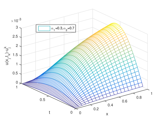
Figure 5.1: The evolutions of the absolute errors obtained by the numerical algorithm (11), together with (12) and (13) for $(\alpha_{1},\alpha_{2})=(0.3,0.7)$ when $\tau=\frac{1}{20}$ and $h=\frac{1}{50}$.

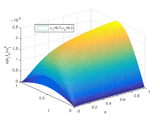
Figure 5.2: The evolutions of the absolute errors obtained by the numerical algorithm (11), together with (12) and (13) for $(\alpha_{1},\alpha_{2})=(0.7,0.3)$ when $\tau=\frac{1}{200}$ and $h=\frac{1}{200}$.

 Example 5.3

Consider the following two-dimensional fractional cable equation:

$$\begin{array}[]{rrr}\displaystyle\frac{\partial u(x,y,t)}{\partial t}=\frac{1}{\pi^{8}}\,_{\mathrm{RL}}{{{\mathrm{D}}}}_{0,t}^{1-\alpha_{1}}\left(\frac{\partial^{2}u(x,y,t)}{\partial x^{2}}+\frac{\partial^{2}u(x,y,t)}{\partial y^{2}}\right)-\,_{\mathrm{RL}}{{{\mathrm{D}}}}_{0,t}^{1-\alpha_{2}}u(x,y,t)\vspace{0.2 cm}\\ +f(x,y,t),\;(x,y;t)\in\Omega\times[0,1],\end{array}$$

with initial value condition

$$\begin{array}[]{lll}\displaystyle u(x,y,0)=0,\;\;(x,y)\in\Omega,\end{array}$$

and boundary value conditions

$$\begin{array}[]{lll}\displaystyle u(x,y,t)=0,\;(x,y)\in\partial\Omega,\;t\in(0,1],\end{array}$$

where the spatial domain $\Omega=(0,1)\times(0,1)$, and the source term is chosen as $f(x,y,t)=2\left(t+\frac{2t^{1+\gamma_{1}}}{\pi^{6}\Gamma(2+\gamma_{1})}+\frac{t^{1+\gamma_{2}}}{\Gamma(2+\gamma_{2})}\right)\sin\pi x\sin\pi y$. The analytical solution is $u(x,t)=t^{2}\sin\pi x\sin\pi y$.

Table 3 lists the computed errors, the temporal and spatial convergence orders respectively, which shows that the convergence order of our scheme (21)–(23) is $\mathcal{O}\left(\tau^{2}+h_{x}^{4}+h_{y}^{4}\right)$. Finally, Figs. 5.3 and 5.4 show the evolutions of the absolute errors for Example 5.3 with different orders, temporal and spatial stepsizes, respectively. It can be seen that the numerical results are in good agreement with the theoretical results.

Table 3: The absolute errors (TAE), temporal convergence order (TCO) and spatial convergence order (SCO) of Example 3 by using difference scheme (21), together with (22) and (23).

$(\alpha_{1},\alpha_{2})$	$\tau$, $h_{x},h_{y}$	TAE	TCO	SCO
$(0.2,0.8)$	$\tau=\frac{1}{5},h_{x}=h_{y}=\frac{1}{5}$	3.822113e-02	—	—
	$\tau=\frac{1}{20},h_{x}=h_{y}=\frac{1}{10}$	3.444335e-03	1.7360	3.4721
	$\tau=\frac{1}{45},h_{x}=h_{y}=\frac{1}{15}$	6.972544e-04	1.9698	3.9395
	$\tau=\frac{1}{80},h_{x}=h_{y}=\frac{1}{20}$	2.254541e-04	1.9623	3.9246
	$\tau=\frac{1}{125},h_{x}=h_{y}=\frac{1}{25}$	2.254541e-04	1.9983	3.9966
$(0.4,0.6)$	$\tau=\frac{1}{5},h_{x}=h_{y}=\frac{1}{5}$	3.460010e-02	—	—
	$\tau=\frac{1}{20},h_{x}=h_{y}=\frac{1}{10}$	2.710859e-03	1.8370	3.6740
	$\tau=\frac{1}{45},h_{x}=h_{y}=\frac{1}{15}$	5.372495e-04	1.9959	3.9919
	$\tau=\frac{1}{80},h_{x}=h_{y}=\frac{1}{20}$	1.726387e-04	1.9731	3.9462
	$\tau=\frac{1}{125},h_{x}=h_{y}=\frac{1}{25}$	7.057381e-05	2.0044	4.0088
$(0.5,0.5)$	$\tau=\frac{1}{5},h_{x}=h_{y}=\frac{1}{5}$	3.379936e-02	—	—
	$\tau=\frac{1}{20},h_{x}=h_{y}=\frac{1}{10}$	2.584901e-03	1.8544	3.7088
	$\tau=\frac{1}{45},h_{x}=h_{y}=\frac{1}{15}$	5.099957e-04	2.0015	4.0029
	$\tau=\frac{1}{80},h_{x}=h_{y}=\frac{1}{20}$	1.636407e-04	1.9757	3.9513
	$\tau=\frac{1}{125},h_{x}=h_{y}=\frac{1}{25}$	6.684963e-05	2.0059	4.0119
$(0.6,0.4)$	$\tau=\frac{1}{5},h_{x}=h_{y}=\frac{1}{5}$	3.295086e-02	—	—
	$\tau=\frac{1}{20},h_{x}=h_{y}=\frac{1}{10}$	2.514903e-03	1.8559	3.7117
	$\tau=\frac{1}{45},h_{x}=h_{y}=\frac{1}{15}$	4.945015e-04	2.0056	4.0113
	$\tau=\frac{1}{80},h_{x}=h_{y}=\frac{1}{20}$	1.584782e-04	1.9778	3.9555
	$\tau=\frac{1}{125},h_{x}=h_{y}=\frac{1}{25}$	6.470169e-05	2.0073	4.0146
$(0.8,0.2)$	$\tau=\frac{1}{5},h_{x}=h_{y}=\frac{1}{5}$	4.721574e-02	—	—
	$\tau=\frac{1}{20},h_{x}=h_{y}=\frac{1}{10}$	2.866291e-03	2.0210	4.0420
	$\tau=\frac{1}{45},h_{x}=h_{y}=\frac{1}{15}$	5.133508e-04	2.1208	4.2416
	$\tau=\frac{1}{80},h_{x}=h_{y}=\frac{1}{20}$	1.543393e-04	2.0888	4.1775
	$\tau=\frac{1}{125},h_{x}=h_{y}=\frac{1}{25}$	6.292841e-05	2.0103	4.0205

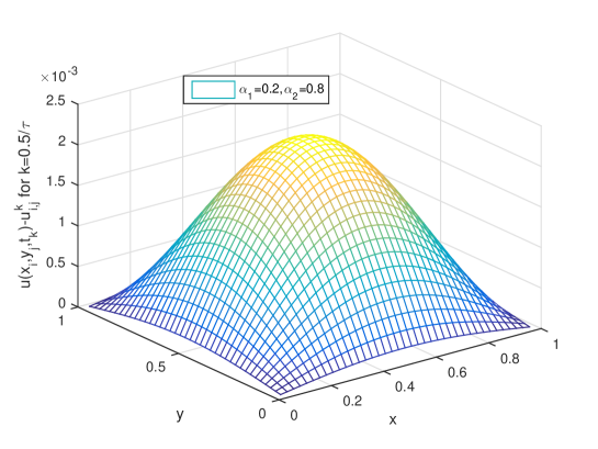
Figure 5.3: The evolutions of the absolute errors obtained by the numerical algorithm (21), together with (22) and (23) for $(\alpha_{1},\alpha_{2})=(0.2,0.8)$ at $t=0.5$ when $\tau=\frac{1}{20}$ and $h=\frac{1}{40}$.

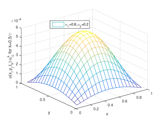
Figure 5.4: The evolutions of the absolute errors obtained by the numerical algorithm (21), together with (22) and (23) for $(\alpha_{1},\alpha_{2})=(0.8,0.2)$ at $t=0.5$ when $\tau=\frac{1}{40}$ and $h=\frac{1}{20}$.

6 Conclusions

In this paper, two classed high-order numerical algorithms are derived to solve the one- and two-dimensional fractional Cable equations based on the derived new second-order difference operator in time direction and the compact techniques in space direction. By using the energy method, we proved that our difference schemes are unconditionally stable to the initial values. The temporal, spatial convergence orders can reach two and four respectively. Finally, numerical examples are given to show the effectiveness of the derived numerical algorithms.

References

- [1] A.A. Alikhanov, A new difference scheme for the fractional diffusion equation, J. Comput. Phys., 280 (2015), 424–438.
- [2] D. Baleanu, O. Defterli, O.P. Agrawal, A central difference numerical scheme for fractional optimal control problems, J. Vib. Control., 15 (2009), 583–597.
- [3] D. Benson, S.W. Wheatcraft, M.M. Meerschaert, The fractional-order governing equation of Lévy motion, Water Resour. Res., 36 (2000), 1413–1423.
- [4] M. Cui, Convergence analysis of high-order compact alternating direction implicit schemes for the two-dimensional time fractional diffusion equation, Numer. Algorithms, 62 (2013), 383–409.
- [5] H.F. Ding, C.P. Li, Y.Q. Chen, High-order Algorithms for Riesz Derivative and Their Applications (I), Abstract and Applied Analysis, Article ID 653797, 2014, 17 pages.
- [6] H.F. Ding, C.P. Li, Y.Q. Chen, High-order algorithms for Riesz derivative and their applications (II), J. Comput. Phys., 293 (2015), 218–237.
- [7] V.J. Ervin, J.P. Roop, Variational formulation for the stationary fractional advection dispersion equation, Numer. Meth. Part. D. E., 22 (2005), 558–576.
- [8] G.H. Gao, Z.Z. Sun, A compact finite difference scheme for the fractional sub-diffusion equations, J. Comput. Phys., 230 (2011), 586–595.
- [9] X.L. Hu, L.M. Zhang, Implicit compact difference schemes for the fractional cable equation, Appl. Math. Model., 36 (2012), 4027–4043.
- [10] X. Jin, Preconditioning Techniques for Toeplitz Systems, Higher Education Press, Beijing, 2010.
- [11] B. Jin, R. Lazarov, J. Pasciak, Z. Zhou, Error analysis of a finite element method for the space-fractional parabolic equation, SIAM. J. Numer. Anal., 52 (2014), 2272–2294.
- [12] C.C. Ji, Z.Z. Sun, The high-order compact numerical algorithms for the two-dimensional fractional sub-diffusion equation, Appl. Math. Comput., 269 (2015), 775–791.
- [13] A.J. Laub, Matrix Analysis for Scientists and Engineers, Society for Industrial and Applied Mathematics, Philadelphia, PA, 2005.
- [14] F. Liu, V. Anh, I. Turner, Numerical solution of the space fractional Fokker-Planck equation, J. Comput. Appl. Math., 166 (2004), 209–219.
- [15] C.P. Li, H.F. Ding, Higher order finite difference method for the reaction and anomalous-diffusion equation, Appl. Math. Model., 38 (2014), 3802–3821.
- [16] T.A.M. Langlans, B. Henry, S. Wearne, Solution of a fractional Cable equation: finite case, Preprint, Submitted to Elsevier Science http://www.maths.unsw.edu.au/applied/filed/2005/amr05-33 (2005).
- [17] Y.M. Lin, X.J. Li, C.J. Xu, Finite difference/spectral approximations for the fractional Cable equation, Math. Comput., 80 (2011), 1369–1396 .
- [18] R. Metler, J. Klafter, The random walk’s guide to anomalous diffusion: a fractional dynamics approach, Phys. Rep., 339 (2000), 1–77.
- [19] R. Metler, J. Klafter, The restaurant at the end of random walk: recent developments in the description of anomalous transport by fractional dynamics, J. Phys. A., 37 (2004), R161–R208.
- [20] F. Mainardi, M. Raberto, R. Gorenflo, E. Scalas, Fractional calculus and continuous-time finance I: the waiting-time distribution, Physica A., 287 (2000), 468–481.
- [21] M.M. Meerschaert, C. Tadjeran, Finite difference approximations for fractional advection-dispersion flow equations, J. Comput. Appl. Math., 172 (2004), 65–77.
- [22] J. Quintana-Murillo, S.B. Yuste, An explicit numerical method for the fractional cable equation, Int. J. Differ. Equ., Article ID 231920, 2011, 12 pages.
- [23] I. Podlubny, Fractional Differential Equations, Academic Press, San Diego, 1999.
- [24] I. Podlubny, A. Chechkin, T. Skovranek, Y. Chen, B. M. V. Jara, Matrix approach to discrete fractional calculus. II. Partial fractional differential equations, J. Comput. Phys., 228 (2009), 3137–3153.
- [25] A. Quarteroni, R. Sacco, F. Saleri, Numerical Mathematics, Springer, New York, 2007.
- [26] I.M. Sokolov, J. Klafter, From diffusion to anomalous diffusion: a century after Einstein’s Brownian motion, Chaos, 15 (2005), 026103.
- [27] S.G. Samko, A.A. Kilbas, O.I. Marichev, Fractional Integrals and Derivatives: Theory and Applications, Gordon and Breach, 1993.
- [28] S. Shen, F. Liu, Q. Liu, V. Anh, Numerical simulation of anomalous infiltration in porous media, Numer. Algorithms, 68 (2015), 443–454.
- [29] T. Wang, B. Guo, A robust semi-explicit difference scheme for the Kuramoto-Tsuzuki equation, J. Comput. Appl. Math., 233 (2009), 878–888.
- [30] Z.B. Wang, S. Vong, Compact difference schemes for the modified anomalous fractional sub-diffusion equation and the fractional diffusion-wave equation, J. Comput. Phys., 277 (2014), 1–15.
- [31] H. Wang, D. Yang, Well posedness of variable-coefficient conservative fractional elliptic differential equations, SIAM. J. Numer. Anal., 51 (2013), 1088–1107.
- [32] M. Zheng, F. Liu, I. Turner, V. Anh, A novel high order space-time spectral method for the time-fractional Fokker-Planck equation, SIAM. J. Sci. Comput., 37 (2015), 701–724.
- [33] P. Zhuang, F. Liu, I. Turner, V. Anh, Galerkin finite element method and error analysis for the fractional Cable equation, Numer. Algorithms, DOI 10.1007/s11075-015-0055-x.
- [34] M. Zayernouri, G.E. Karniadakis, Discontinuous spectral element methods for time-and space-fractional advection equations, SIAM. J. Sci. Comput., 36 (2014), B684–B707.