Two-parameter scaling theory of the longitudinal magnetoconductivity in a Weyl metal phase: Chiral anomaly, weak disorder, and finite temperature
Abstract
It is at the heart of modern condensed matter physics to investigate the role of a topological structure in anomalous transport phenomena. In particular, chiral anomaly turns out to be the underlying mechanism for the negative longitudinal magnetoresistivity in a Weyl metal phase. Existence of a dissipationless current channel causes enhancement of electric currents along the direction of a pair of Weyl points or applied magnetic fields (). However, temperature () dependence of the negative longitudinal magnetoresistivity has not been understood yet in the presence of disorder scattering since it is not clear at all how to introduce effects of disorder scattering into the “topological-in-origin” transport coefficient at finite temperatures. The calculation based on the Kubo formula of the current-current correlation function is simply not known for this anomalous transport coefficient. Combining the renormalization group analysis with the Boltzmann transport theory to encode the chiral anomaly, we reveal how disorder scattering renormalizes the distance between a pair of Weyl points and such a renormalization effect modifies the topological-in-origin transport coefficient at finite temperatures. As a result, we find breakdown of scaling, given by with . This breakdown may be regarded to be a fingerprint of the interplay between disorder scattering and topological structure in a Weyl metal phase.
I Introduction
Researches on the role of topological-in-origin terms in quantum phases and their transitions have been a driving force for modern condensed matter physics, which cover quantum spin chains 1D_QFT_Textbook and deconfined quantum criticality DQCP_Senthil ; DQCP_Tanaka , quantum Hall effects and topological phases of matter Fradkin_Textbook , Anderson localization for the classification of topological phases and their phase transitions Mirlin_Review , and so on. In particular, renormalization effects of such topological terms are responsible for novel universality classes beyond the Landau-Ginzburg-Wilson paradigm of phase transitions with symmetry breaking. However, it is quite a nontrivial task to perform the renormalization group analysis in the presence of the topological-in-origin term, even if it can be taken into account perturbatively for the contribution of a bulk sometimes. Frequently, non-perturbative effects should be introduced into the renormalization group analysis PP_Transition_IQHE ; Fu_Kane_NLsM , uncontrolled in this situation and thus, being under debates as an open question.
In this study we investigate disorder-driven renormalization of a topological-in-origin term referred to as an inhomogeneous term in three spatial dimensions WM_Review_Kim , defined by
| (1) |
is a four-component Dirac spinor to describe an electron field of spin in two orbitals. Its dynamics is given by a Dirac theory, where with is a Dirac matrix to satisfy the Clifford algebra. and are an externally applied electromagnetic field and its field strength tensor, respectively. is a potential configuration, given randomly and described by the Gaussian probability distribution . is the variance of the disorder distribution and is a normalization constant, determined by . The last term is an inhomogeneous term, topological in its origin and keeping chiral anomaly that the chiral current is not conserved in the quantum level QFT_Textbook , given by
is chiral Dirac matrix to anticommute with . Here, the problem is how the inhomogeneous term becomes renormalized via the disorder scattering.
This problem can be cast into more physical terms. Introducing the chiral-anomaly equation into the effective field theory and performing the integration-by-parts for the chiral-current term with the coefficient Kyoung , we obtain
| (3) |
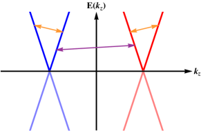
is referred to as chiral gauge field, regarded to be a background potential given by the inhomogeneous coefficient. When the background chiral gauge field serves a homogeneous potential, the resulting spectrum turns out to describe dynamics of Weyl electrons. The right-handed helicity part shifts into the right hand side and the left-handed helicity part does into the left Weyl_Metal_I ; Weyl_Metal_II ; Weyl_Metal_III . Physically, this homogeneous chiral-gauge-field potential is realized as , applying a homogeneous magnetic field into a gapless semiconductor described above. The Dirac point separates into a pair of Weyl points along the direction of the applied magnetic field and the distance of the pair of Weyl points is proportional to the strength of the applied magnetic field with a Lande factor. See the supplementary material. As a result, the previous mathematically defined problem is actually how the background chiral gauge field, more physically, the distance between a pair of Weyl points becomes renormalized by random elastic scattering.
The renormalization effect of the distance between a pair of Weyl points is measurable experimentally since the information is encoded into the negative longitudinal magnetoresistivity. This anomalous transport phenomena in a Weyl metal phase has been well known for more than thirty years NLMR_Theory_Original and experimentally confirmed firstly in 2013 NLMR_Experiment_Original . The electrical resistivity measured along the direction of the applied magnetic field becomes smaller than that measured in other directions. More quantitatively, the magnetoconductivity is enhanced in the longitudinal setup, i.e., , as follows
| (4) |
where is an applied electric field Boltzmann_Spivak_Tong . is the Drude conductivity determined purely by disorder scattering. In real experiments, quantum corrections by weak anti-localization are introduced into the Drude conductivity Boltzmann_Kim_I . is a positive coefficient, discussed later in more detail. An essential point is that the enhancement of the longitudinal magnetoconductivity is given by the square of the distance between the pair of Weyl points. This longitudinal enhancement can be figured out in the following way: There exists a dissipationless current channel as a vacuum state, which connects the pair of Weyl points, responsible for the chiral anomaly. As a result, electrical currents are allowed to flow better along this direction through this vacuum channel although the measured longitudinal magnetoconductivity does not result from such dissipationless electrical currents NLMR_Theory_Original . When the distance between the pair of Weyl points is renormalized by random elastic scattering, the positive coefficient would evolve as a function of an energy scale, here, temperature. It is natural to expect finding a scaling theory for the chiral-anomaly-driven enhanced longitudinal magnetoconductivity.
The above discussion reminds us of a two-parameter scaling theory for the Anderson localization in topological phases of matter Altland_Two_Parameter_Scaling , including the plateau-plateau transition in the integer quantum Hall effect PP_Transition_IQHE . There, the transport phenomenon of the Anderson localization transition is determined by the “transverse” conductivity and the Hall conductivity , where the latter encodes the topological information of the integer quantum Hall effect. The present situation is quite analogous to that of the integer quantum Hall effect. in the quantum Hall effect is identified with the Drude conductivity , determined by disorder scattering directly. On the other hand, in the quantum Hall effect is analogous to the distance between the pair of Weyl points, where the renormalization effect is introduced into the temperature dependence of .
In this study we investigate the longitudinal magnetoconductivity at finite temperatures and find a two-parameter scaling theory, where renormalization effects result from random elastic scattering. There is one difficult point in the calculation of the longitudinal magnetoconductivity in a Weyl metal phase. It turns out that a naive Kubo-formula calculation does not incorporate the role of the chiral anomaly in the longitudinal magnetoconductivity TFLT_Kim . As a result, we fail to find the enhancement of the longitudinal magnetoconductivity within the Kubo-formula calculation. In this respect our strategy consists of a two-fold way: First, we perform the renormalization group analysis and find how the distance between a pair of Weyl points evolves as a function of an energy scale or temperature. Second, introducing this information into the Boltzmann transport theory with chiral anomaly, we reveal the longitudinal negative magnetoconductivity as a function of both the applied magnetic field and temperature, given by
| (5) |
In particular, we find breakdown of scaling
where is a scaling exponent with and is an energy scale. We claim that this breakdown may be regarded to be a fingerprint of the interplay between disorder scattering and topological structure in a Weyl metal phase.
II Renormalization for the distance between a pair of Weyl points via disorder-driven inter-valley scattering
II.1 Effective field theory for a Weyl metal phase with disorder: Replica theory
We start from an effective Hamiltonian density for a Weyl metal phase with time reversal symmetry breaking
| (7) |
is a four-component Dirac-spinor field in a two-component Weyl-spinor field with right(R)-left(L) chirality, and is the velocity of such fermions. is an externally applied magnetic field with a Lande factor , splitting the Dirac band into a pair of Weyl bands (Fig. 1). is a four-by-four matrix, given by , where is a Pauli matrix. The subscript denotes “bare”, meaning that this effective Hamiltonian density is defined at an ultraviolet (UV) scale.
We consider two types of random potentials, introducing “intra-valley scattering” and “inter-valley scattering” into the effective Hamiltonian. Then, we obtain the following effective action
| (8) |
with . Here, gamma matrices are given in the Weyl representation, for example, . A magnetic field is generalized to be a chiral gauge field . means “space-time”, given by . See the supplementary material.
A physical observable in this system is measured as follows
| (9) |
where the free part of the effective action is . Resorting to the replica trick and performing the average for disorder with the Gaussian distribution function of , the above expression is reformulated as follows
| (10) |
Here, is a normalization constant and is a variance for the disorder distribution. As a result, the effective interaction term induced by disorder scattering is
| (11) | |||||
The effective field theory is given by .
II.2 Renormalization group analysis: Role of inter-valley scattering in the distance between a pair of Weyl point
In order to perform the renormalization group analysis within the dimensional regularization QFT_Textbook , we rewrite , the effective bare action of bare field variables in terms of , the effective renormalized action of renormalized field variables with , counter terms of renormalized field variables
where . It is straightforward to see how bare quantities are related with renormalized ones, given by
| (13) |
where , , , , , and .
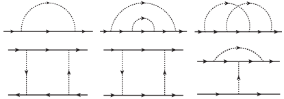
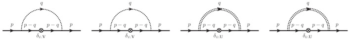
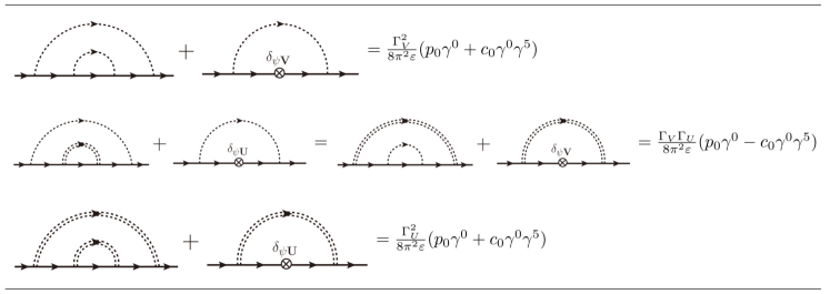
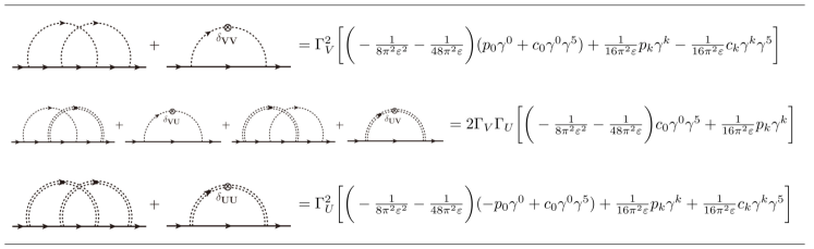
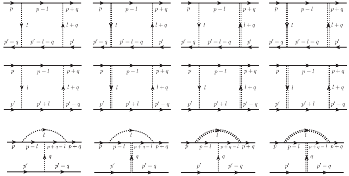
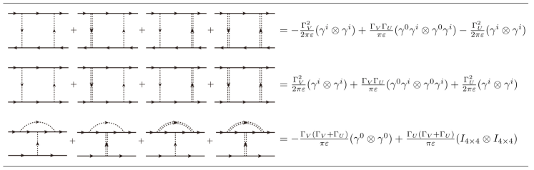
Dimensional analysis gives . In this respect we perform the dimensional regularization in where , a “small” parameter to control the present renormalization group analysis, will be analytically continued to in the end. Performing the standard procedure for the renormalization group analysis, we find renormalization group equations, where both vertex and self-energy corrections are introduced self-consistently. See Fig. 2, where all quantum corrections are shown as Feynman’s diagrams up to the two-loop order for self-energy corrections and the one-loop order for vertex corrections. All details are shown in the supplementary material. As a result, we find counter terms with
| (14) | |||||
Inserting these divergent coefficients into equations (13) and performing derivatives with respect to an energy scale for renormalization given by , we find renormalization group equations
| (15) | |||||
where positive numerical constants are given by
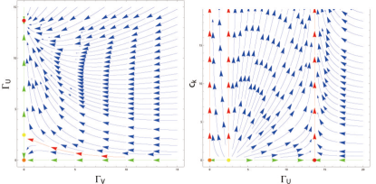
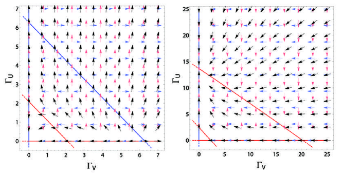
Fig. 3 shows renormalization group flows for physical parameters according to Eq. (15). In the plane of , we find two stable fixed points corresponding to two phases of a disordered Weyl metal state, and one unstable fixed point corresponding to the phase transition point between two phases: (1) The stable fixed point of with represents a clean Weyl metal phase, protected for the case of weak disorder by the pseudogap density of states of the Weyl metal state. (2) The stable fixed point of with is identified with a diffusive Weyl metal phase, analogous to the diffusive Fermi-liquid fixed point of a conventional metallic phase CMP_QFT_Textbook . (3) The unstable fixed point of with denotes a critical point to separate the diffusive Weyl metal phase from the clean Weyl metal state, the existence of which originates from the pseudogap density of states. Interestingly, all these fixed points lie at the line of , which means that inter-valley scattering shows dominant effects over intra-valley scattering for the low-energy physics in the disordered Weyl metallic state. Naively, one may suspect that their roles are similar because of the similarity of their renormalization group equations. However, the magnitude of the one-loop correction for turns out to be three times larger than that for , and thus, the renormalization group flow of is overwhelmed by . As a result, there is no chance by which has a non-trivial fixed point value. Detailed analysis on this issue is given in the supplementary material (Fig. 16).
In order to figure out how the distance between the pair of Weyl points renormalizes as a function of an energy scale, we focus on renormalization group equations for and at
| (16) | |||||
| (17) |
It is straightforward to solve the first equation and find an approximate solution for near each fixed point at . Inserting such fixed-point solutions into the second equation, we uncover how the distance between the pair of Weyl points evolves as a function of temperature
| (18) |
where the energy scale has been replaced with temperature . Critical exponents of are found to be
| (19) | |||||
| (20) | |||||
| (21) |
It turns out that the distance between a pair of Weyl points increases to reach infinity, regarded to be beyond the perturbative renormalization group analysis. However, the infinity should be considered as an artifact of the continuum approximation. If the Brillouin zone is taken into account in the effective field theory, there must be a maximum of the distance within the Brillouin zone. In this respect it is natural to modify the above scaling solution as follows
| (22) |
where is a cutoff scale in the low-energy limit. It is interesting to notice that disorder scattering changes the temperature-dependent exponent of . Inter-valley scattering gives rise to fast enhancement of the distance between a pair of Weyl points at low temperatures. This looks counter-intuitive, where anti-screening instead of screening arises from inter-valley scattering.
III Two-parameter scaling theory for the longitudinal magnetoconductivity of a disordered Weyl metal phase within Boltzmann transport theory
The question to address in this study is to find a scaling theory for the longitudinal magnetoconductivity. As discussed in the introduction, not only the Drude conductivity but also the distance between a pair of Weyl points or the spatial gradient of the inhomogeneous coefficient in the topological-in-origin term should be taken into account for the longitudinal magnetoconductivity in the Weyl metal phase. This situation is analogous to that of a plateau-plateau transition in the integer quantum Hall effect: Not only the Drude conductivity but also the Hall conductivity, a topological term, should be considered on equal footing in order to describe such a quantum phase transition involved with Anderson localization. In this respect we call the scaling theory for the longitudinal magnetoconductivity of a disordered Weyl metal phase two-parameter scaling theory as the Anderson localization transition in the case of the quantum Hall effect.
Previously, we found and , based on the perturbative renormalization group analysis, where gives the Drude conductivity and describe the enhancement of the longitudinal magnetoconductivity. More precisely, we can address renormalization effects of the longitudinal magnetoconductivity based on the Boltzmann transport theory for a Weyl metal phase Boltzmann_Kim_I ; Boltzmann_Kim_II
| (23) |
Here, is the distribution function at a chiral Fermi surface denoted by , where is the relative momentum of a particle-hole pair near the chiral Fermi surface, and and are the center of mass position and time of the particle-hole pair.
and represent the change of position and momentum with respect to time, classically described and given by the so called modified Drude model AHE_Review_I ; AHE_Review_II
| (24) |
represents a momentum-space magnetic field on the chiral Fermi surface, resulting from a momentum-space magnetic charge enclosed by the chiral Fermi surface. We would like to recall that the Berry curvature does not appear on the “normal” Fermi surface that does not enclose a band-touching point. As a result, we reproduce the Drude model with . It is essential to realize the following relation between the applied magnetic field and the distance between the pair of Weyl points
| (25) |
It is straightforward to solve these coupled equations, the solution of which is
where is a volume factor of the modified phase space with a pair of momentum-space magnetic charges . They are well known the role of anomalous electromagnetic-field-dependent terms in anomalous transport phenomena: (1) The second term of in the first equation is responsible for the anomalous Hall effect, the Hall effect without an applied magnetic field due to an emergent magnetic field referred to as Berry curvature in the momentum space AHE_I ; AHE_II ; AHE_III . (2) The third term of in the first equation gives rise to the so called chiral magnetic effect that dissipationless electric currents are driven by applied magnetic fields in the limit of vanishing applied electric fields, proportional to the distance between the pair of Weyl points or applied magnetic fields CME_I ; CME_II ; CME_III ; CME_IV ; CME_V ; CME_VI . (3) The third term of in the second equation causes the gauge anomaly for electrons on each chiral Fermi surface that gauge or electric currents on each chiral Fermi surface are not conserved NLMR_Theory_Original ; NLMR_Experiment_Original ; Boltzmann_Spivak_Tong ; Boltzmann_Kim_I ; Boltzmann_Kim_II ; CME_II ; CME_III ; ABJ_Anomaly_I ; ABJ_Anomaly_II ; ABJ_Anomaly_III ; ABJ_Anomaly_IV ; ABJ_Anomaly_V ; ABJ_Anomaly_VI ; ABJ_Anomaly_VII ; ABJ_Anomaly_VIII . Of course, the breakdown of the gauge symmetry should be cured when total electric currents are considered, but chiral “electric” currents are still not conserved, referred to as chiral anomaly.
The collision part is given by
| (27) | |||||
The first term describes the intra-valley scattering, and the second represents the inter-valley scattering. In this respect both scattering rates of and correspond to and , respectively.
Considering homogeneity of the Weyl metal phase under constant electric fields in the dc-limit, we are allowed to solve . As a result, we find a two-parameter scaling theory for the longitudinal magnetoconductivity in a disordered Weyl metal phase
| (28) |
where is the Drude conductivity inversely proportional to and is the distance between a pair of Weyl points.
Rewriting the distance between the pair of Weyl points as , we consider
| (29) | |||||
for the universal scaling relation. More explicitly, inserting into the above, we find
| (30) |
where “anomalous dimensions” are given by and , respectively, for each fixed point.
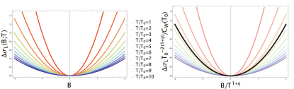
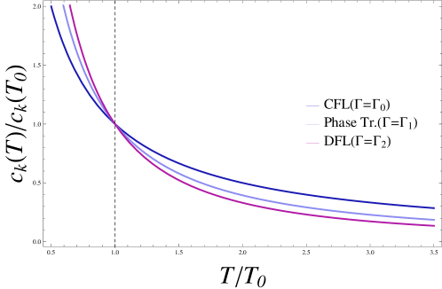
Fig. 4 shows the longitudinal magnetoconductivity, enhanced to be proportional to , the square of the distance between the pair of Weyl points, at each temperature. Our renormalization group analysis confirms that the distance between the pair of Weyl points is renormalized to increase, lowering temperature, i.e., with . As a result, the degree of enhancement becomes larger as temperature is reduced (Left). Interestingly, these longitudinal transport coefficients turn out to be collapsed into a single universal curve, described by Eq. (30) (Right).
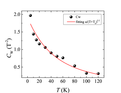
Fig. 5 shows the comparison between from an experimental data of with and that from our renormalization group analysis WM_Review_Kim ; Exp_in_preparation . Experimentally, the enhancement coefficient can be found from fitting the experimental data with Eq. (5) at a given temperature, where the Drude part is replaced with a transport coefficient of weak anti-localization corrections and additional contributions, which have nothing to do with Weyl points, are also introduced NLMR_Experiment_Original . Repeating this fitting procedure for various temperatures, we obtain the temperature dependence of . The comparison between the experimental and the renormalization group analysis Eq. (30) looks appealing.
IV Discussion and conclusion
The original motivation of the present study is to reveal the existence of a topological phase transition from a Weyl metal phase to a normal metal state as a function of the strength of disorder and temperature. Our physical picture for this phase transition is as follows. Disorder scattering, in particular, inter-valley scattering is expected to kill the nature of the Weyl metallic phase since it induces mixing of chirality. We recall that the inter-valley scattering appears as an effective random-mass term. If has a nontrivial vacuum expectation value, i.e., , expected to realize in the case of sufficiently strong disorder, the chiral symmetry breaks down even at the classical level and the chiral anomaly loses the physical meaning. As a result, we speculate that the distance between the pair of Weyl points renormalizes to vanish. A diffusive normal metallic state would be realized in the case of sufficiently strong disorder. Since this phase transition is not involved with symmetry breaking, it is identified with a topological phase transition.
This topological phase transition may be translated into Peccei-Quinn symmetry breaking in the context of dynamical generation of axions PQSB ; PQSB_Review . In order to realize the Peccei-Quinn symmetry breaking, there must be a scalar field. When the scalar field does not have its vacuum expectation value, any value of the angle can be canceled by the Peccei-Quinn transformation. On the other hand, the Peccei-Quinn symmetry breaking occurs when the scalar field has its vacuum expectation value. As a result of the continuous symmetry breaking, there exists a Goldstone boson field, referred to as an axion field. When the Peccei-Quinn symmetry is exact and thus, the axion field is massless, any value of the angle can be still canceled by the Peccei-Quinn transformation. However, there are instanton excitations, which do not allow the Peccei-Quinn symmetry not to be exact, giving rise to a mass term in the axion dynamics. Then, the vacuum angle is fixed to be , minimizing the energy of the system. In the present situation the corresponding scalar field results from the Hubbard-Stratonovich transformation of the random-mass term in the replica effective field theory, conventionally referred to as , where and denote the replica index. However, there are two different aspects between the possible topological phase transition and the Peccei-Quinn symmetry breaking in high energy physics: (1) The vacuum angle is given by an inhomogeneous function of position while its gradient identified with a chiral gauge field is a constant. (2) There are no instanton-type excitations in the Weyl metal phase. This direction of research would be an interesting future task.
Unfortunately, the perturbative renormalization group analysis fails to access such an unstable fixed point, identified with the quantum critical point of the topological phase transition. In this respect the naming of the two-parameter scaling theory is not satisfactory in our opinion, basically motivated from the analogy with the plateau-plateau transition in the integer quantum Hall effect. However, it turns out that the longitudinal magnetoconductivity is governed by both parameters of the Drude conductivity and the distance between the pair of Weyl points, renormalized by inter-valley scattering, essentially analogous to and in the quantum Hall effect, respectively. In this respect we may call what we performed two-parameter scaling theory for the longitudinal magnetoconductivity in a disordered Weyl metal phase.
An unexpected result is breakdown of the scaling behavior near the diffusive fixed point although it is fulfilled near the clean fixed point. Actually, we could verify this prediction, comparing the proposed formula Eq. (30) of the two-parameter scaling theory with in the experimental data of with . Here, we took into account modifying the original renormalization group analysis, introducing a cutoff scale into the equation for the distance between the pair of Weyl points as Eq. (22), in order to prohibit the divergence of the length scale within the Brillouin zone. This breakdown may be regarded to be a fingerprint of the interplay between disorder scattering and topological structure in a Weyl metal phase.
Acknowledgement
This study was supported by the Ministry of Education, Science, and Technology (No. NRF-2015R1C1A1A01051629 and No. 2011-0030046) of the National Research Foundation of Korea (NRF) and by TJ Park Science Fellowship of the POSCO TJ Park Foundation. This work was also supported by the POSTECH Basic Science Research Institute Grant (2015). We would like to appreciate fruitful discussions in the APCTP workshop on Delocalisation Transitions in Disordered Systems in 2015.
Appendix A model hamiltonian
A minimal model for a Weyl metal state is given by
is a four-component Dirac-spinor field in a two-component Weyl-spinor field with right(R)-left(L) chirality, and is the velocity of such fermions. is an electron chemical potential. is an externally applied magnetic field with a Lande factor . is a four-by-four matrix, given by , where is a Pauli matrix.
First, we look into a band structure. This block-diagonal matrix can be diagonalized as
where and are projection matrices, and is an eigenstate. The unitary matrix varying with is given by
where is the polar (azimuthal) angle of , respectively. If we draw a band structure along some momentum-line, for example, , then we obtain a pair of Weyl cones as shown in Fig. 1.
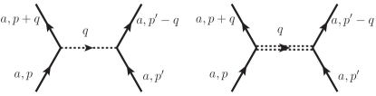
Second, we consider two types of random potentials, say, “intra-valley scattering” and “inter-valley scattering”, given by
where and are disorder potentials for intra-valley scattering and inter-valley scattering, respectively.
Now, the effective action is
where the corresponding free energy is given by in a given configuration of random potentials. We represent this effective action in terms of gamma matrices in the Weyl representation
Then, we reach the following expression
with an adjoint spinor-field , where we introduced with “time-component” . “Space-time” of is and other four-vectors are defined, similarly. For example, four-momentum is with . Since the action has been formulated in the imaginary time, it is defined on the Euclidean geometry as shown by .
Appendix B effective field theory for renormalization group analysis
B.1 Disorder Average
We define the free part of the effective action as
Then, a physical observable is measured as follows
This can be reformulated as
where is a source field coupled to an operator , locally.
In order to perform the averaging procedure for disorders, we resort to the replica trick of
where the replicated partition function is
with a replica index “a”. In this technique a physical observable is given by
In this study we take into account static-and Gaussian-distributed disorders, given by
where is a normalization factor. It is straightforward to perform the Gaussian integral for disorders, resulting in
where disorder-driven effective interactions are [Eq. (11)]
B.2 Renormalized perturbation theory
From now on, we focus on the case of a zero-chemical potential. We start from the following effective action
where summations on the replica indices are implied. The subscript denotes “bare”, meaning that this effective action is defined at an ultraviolet (UV) scale. Note that we have generalized dimensions to “d(space)+1(time)” for dimensional regularization.
Performing the dimensional analysis, where space and time coordinates have in mass dimension, we observe
In this respect we perform the renormalization group analysis in dimensions, where is a “small” parameter. In the end of the calculation the dimensions are analytically continued to the physical dimensions () by setting .
Taking into account quantum corrections, divergences would be generated. They can be absorbed into renormalization constants by redefining fields and parameters. Rewriting the bare action in terms of renormalized fields and couplings, we obtain
where such renormalized fields and parameters are given by
It is more elaborate to represent this theory by separating the renormalized part from counter terms that are to absorb divergences in the following way [Eq. (II.2)],
where , , , , and .
B.3 Feynman Rules
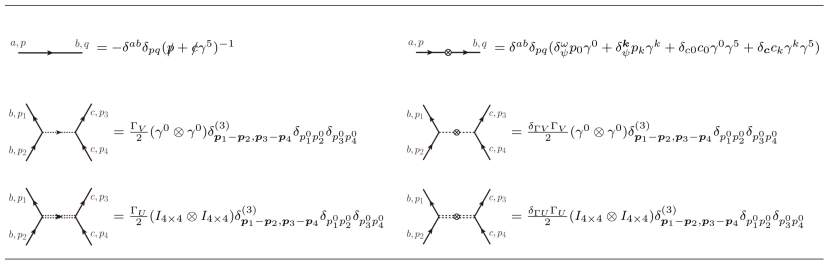
In the momentum and frequency space the effective action is written as
where Feynman rules are given in Fig. 6.
Since there is a chiral gauge field in the kinetic-energy part, the free propagator becomes a little bit complex. Considering the following identity
we obtain an electron Green function
We introduces the following expression with a Feynman parameter for the renormalization group analysis
For a future use, we rearrange it in terms of as
| (31) | |||||
Alternatively, we obtain in terms of
| (32) | |||||
where and . We may use either of these expressions for convenience. Despite their complicated form, they will not be involved much in actual integration procedures.
Appendix C self-energy corrections
C.1 Relevant Feynman’s diagrams
Within the replica trick, we are allowed to perform the perturbative analysis. The full Green function of is evaluated up to the order as follows
where summations on the replica indices are implied. Feynman diagrams whose internal lines are not connected to external lines always vanish due to the replica symmetry (all Green’s functions with different replica indices are identical) and the replica limit (). For details, we refer to Ref. Kyoung .
We find self-energy corrections in the first-order (Fig. 7),
| (33) |
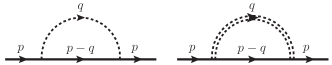
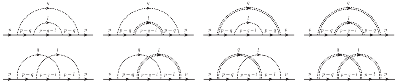
Likewise, we find self-energy corrections in the second order (Fig. 8).
C.2 Evaluation of relevant diagrams
From now on, we evaluate self-energy diagrams one by one. Since there are two types of interactions, we have many diagrams to evaluate, especially, in the two loop-order. Instead of struggling to evaluate them one by one, we’re going to find integration formulae for products of Green functions and make a use of them for the same types of diagrams.
C.2.1 One-loop order: Fock diagrams
First, we evaluate the first-order Fock diagram
where is given by
With Eq. (32), the Green function is given by
where .
Dropping -odd terms, we have
| (36) |
Then, the self-energy is given by
where we have introduced a bar-notation: . Since we perform dimensional regularization in , the term containing gives only a finite value. A relevant part for renormalization is
| (37) | |||||
where -terms vanish after the integration over .
Based on this result, we find propagator counter terms in the following way
As a result, propagator counter terms up to the one-loop level are obtained as
| (38) |
C.2.2 Two-loop order I: Rainbow diagrams
Next, we evaluate the rainbow diagrams
where is given by
We may simplify this expression with as
where we used .
Taking into account
with and resorting to the representation of Eq. (32), we reach the following expression
There are many even terms contributing to the integration. However, it turns out that we have to consider the product of s only. This is because the divergent part of is canceled by the one-loop self-energy diagrams containing the first-order counter term, so only the finite part of participates in the remaining calculation.‡ In other words, divergences may arise only by the -term in the -integration. For now, we just assume it (we will be back to this point later).
Keeping this term only, we have
Then, the second-order self-energy correction for the rainbow diagrams is
When performing the renormalization group analysis in the second order, we should include consistently one-loop self-energy corrections made of a tree-level vertex and a one-loop propagator counter term, given by (Fig. 9)
where means the divergent part of . If we add these to the rainbow diagrams, the divergent part of in the rainbow diagrams is eliminated and only a finite part participates in the remaining computation (so the remark of is proved).
Writing it as , we obtain
An expansion about gives
As a result, the relevant part for renormalization is given as
The remaining calculation is . A straightforward calculation gives
where and , .
Dropping the complex logarithm terms, we have
As a result, the self-energy correction from rainbow diagrams is
| (39) |
where the result is depicted pictorially in Fig. 10.
C.2.3 Two-loop order II: Crossed diagrams
Last, we evaluate the crossed diagrams
where is given by
In this case the loop momenta of and are interwoven and this makes the analysis more complicated.
First, we perform the integration on . Using Eq. (32), we have
Denominators are combined as
where . Shifting and renaming as , we have
Despite this complex expression, we need to consider only a few terms for renormalization. This can be understood, considering a simple integral
| (40) |
Since we resort to the dimensional regularization in , an integral for smaller than gives a finite value, and it doesn’t participate in renormalization. The product of the -terms (i.e. -term) certainly gives renormalization effects. Other than -term, even terms of , and possibly contribute to renormalization after the -integral because there will be an equal number of momentum in the denominator and numerator (considering the dimension of an integrand, this fact may be easily estimated, because any dimensionful constant in numerator lowers the superficial degree of divergence of the integral). All of those come from the product of the -terms, so the relevant part is
where .
The numerator is arranged as
where the coefficients are given by
Now, the integral is easily performed to be
Next, we perform the -integral. Using (since the matrices of and are either or ), we have
Taking out from first, we find that the remaining integrals are such a simple form:
where the cases of correspond to integrals for and , respectively. Such integrations result in , where stands for (the leading even-term) and for a constant term in the propagator. Within the dimensional regularization in , only the integral of possibly gives a divergent factor of . However, in the case we already got , and we need to consider the constant () term, which turns out to be important. We first compute this term.
The denominator is transformed as
where . This suggests that we may use Eq. (32) with a slight change. Then, the integral for is
where is same with that of Eq. (32) except for . Note (the original definition of ) and .
This implies that we may take out a relevant part in the following way
Note that in the first term is canceled after the -integral, but in the second term is not. Together with originating from the -integral, the first term contributes to a divergent part while the other higher-order terms give only finite values. In short, the above analysis suggests that we should include .
Now, we focus on the case. Since may arise from (surely) and (after momentum shift), we’re keeping them. After the similar analysis as the above, we obtain
where we have shifted and kept only the leading even terms including shifted contributions from and .
After the -integration, we reach the following expression
Considering , is not involved in the - and the -integral. The effect of the -integral is just to remove . The -integral gives
where makes up for the difference due to additional . Among the remaining Feynman parameters of and , only is effective since there are polynomials of in the s.
The -integrals for each are performed as (from the first line, )
As a result, we obtain
where we have used the matrix identities:
Finally, the self-energy correction from the crossed diagrams is

When we take into account the vertex renormalization, we should introduce consistently self-energy corrections made of a vertex counter term, given by (Fig. 11)
Recall in Eq. (36).
Expanding about and inserting and into the above expression, which will be computed in the next section, we obtain
Adding these contributions to the crossed diagrams, we finally obtain
| (41) | |||||
This result is depicted pictorially in Fig. 12.
Appendix D vertex correction
D.1 Relevant Feynman diagrams
The vertex renormalization can be found from a four-point function of . Performing the perturbative analysis up to the order, we obtain
Among the first-order contributions, fully-connected diagrams give scattering elements (Fig. 13). The four-point function and the scattering matrix element at the tree level are
| (42) |
Among the second order contributions, only diagrams fully connected with the external lines survive in the replica limit of and give scattering matrix elements. Thus, the scattering matrix elements in the second order are given by (Fig. 14)
where , and represent “particle-hole”, “particle-particle” and “vertex”, respectively.
D.2 Evaluation of relevant diagrams
D.2.1 Particle-hole channel
Using Eq. (31), we have
Despite this complicated expression, only the product of the -cubic terms contributes to renormalization by the same reason that we considered in Eq. (40). Keeping this term only, we obtain
where and .
Renaming momentum as and keeping only a relevant term again, we reach the following expression
Thus, the scattering matrix element for the particle-hole diagrams is
| (43) |
D.2.2 Particle-particle channel
The analysis is quite similar with that of the particle-hole channel. Keeping only a relevant term, we have
where and . Note a minus sign in front of the integral that essentially originates from the opposite sign in the loop-momentum of the two propagators. Due to this sign difference, the contribution from the pp-diagram will cancel that of the ph-diagram.
The remaining calculation is the same as before. As a result, we reach the following expression
Thus, the scattering matrix elements for the particle-particle diagrams is
| (44) |
D.2.3 Vertex channel
The analysis is also similar with the ph case except for the fact that “” are not located between propagators.
Keeping only a relevant term, we have
where and .
Renaming momentum as and keeping only a relevant term again, we reach the following expression
Thus, the scattering matrix element for the vertex-diagrams is
| (45) |
where the result is depicted pictorially in Fig. 15.
Appendix E renormalization group equations
Combining Eq. (37), Eq. (39) and Eq. (41) in the following way
we find propagator counter terms in Eq. (14)
Similarly, combining Eq.(43), Eq.(44) and Eq.(45) as follows
we find vertex counter terms in Eq. (14)
As a result, we obtain the renormalization factors:
| (46) |
where we have replaced with a cut-off scale, , and approximated the renormalization factor as .
Recall the relations between the bare and renormalized quantities: , and . Based on these equations, it is straightforward to find the renormalization group equations
| (47) |
Substituting the results of (46) into Eq. (47), we obtain the renormalization group equations [Eq.(15)]
We notice that and affect renormalization of the other parameters, but the reverse way is not the case. In other words, and determine renormalization effects of all parameters, including themselves. In this respect we focus first on the equations for and :
It turns out that despite their structural similarity of these equations the fates of two types of disorders are very distinct as depicted in Fig. 16. If we include one-loop corrections only (Left), there appear two critical lines each for and . Over the red line starts to increase and over the blue line does, too. However, the total gradient is overwhelmed by that of , i.e. almost upward. This means that the anti-screening of is much weaker than that of . If we include two-loop corrections also that give rise to screening in both disorders (Right), there appears another critical line for while the critical line for disappears, so becomes irrelevant. As a result, we have two nonzero fixed points on the line of as shown in this figure and the first figure in Fig. 3.
This observation suggests that has dominant effects over for the low-energy physics. Since we are interested in the renormalization of , we need to consider two equations at :
where the positive numerical constants are given by
In the first equation for , there are three fixed points: , and . Two stable fixed points of and are identified as a clean Weyl metal state and a diffusive Weyl metal phase, respectively. An unstable fixed point of is identified as the phase transition point from the clean Weyl metal state to the diffusive Weyl metal phase.
Let’s move on the second equation for . The formal solution is given by
where is a UV cutoff. Inserting the solution of into the above, we find that the distance between the pair of Weyl points shows a power-law divergent behavior
| (48) |
where is a critical exponent around each fixed point, given by
Disorder scattering changes the temperature-dependent exponent of (see Fig. 17).
References
- (1) A. O. Gogolin, A. A. Nersesyan, and A. Tsvelik, Bosonization and Strongly Correlated Systems, (Cambridge University Press, New York, 1998).
- (2) T. Senthil, A. Vishwanath, L. Balents, S. Sachdev and M. P. A. Fisher, Science 303, 1490 (2004); T. Senthil, L. Balents, S. Sachdev, A. Vishwanath and M. P. A. Fisher, Phys. Rev. B 70, 144407 (2004).
- (3) A. Tanaka and X. Hu, Phys. Rev. Lett. 95, 036402 (2005).
- (4) E. Fradkin, Field Theories of Condensed Matter Physics, (Cambridge University Press, New York, 2013).
- (5) F. Evers and A. D. Mirlin, Rev. Mod. Phys. 80, 1355 (2008).
- (6) A. M. M. Pruisken, Nucl. Phys. B 235, 277 (1984); A. M. M. Pruisken, Nucl. Phys. B 240, 30 (1984).
- (7) L. Fu and C. Kane, Phys. Rev. Lett. 109, 246605 (2012).
- (8) For a review, see Ki-Seok Kim, Heon-Jung Kim, M. Sasaki, J.-F. Wang, L. Li, Sci. Technol. Adv. Mater. 15, 064401 (2014).
- (9) M. E. Peskin and D. V. Schroeder, An Introduction to Quantum Field Theory, (Addison Wesley, New York, 1995).
- (10) F. D. M. Haldane, Phys. Rev. Lett. 93, 206602 (2004).
- (11) S. Murakami, New J. Phys. 9, 356 (2007).
- (12) A. A. Burkov and L. Balents, Phys. Rev. Lett. 107, 127205 (2011).
- (13) Kyoung-Min Kim, Yong-Soo Jho, and Ki-Seok Kim, Phys. Rev. B 91, 115125 (2015).
- (14) H. B. Nielsen and M. Ninomiya, Phys. Lett. 130B, 389 (1983).
- (15) Heon-Jung Kim, Ki-Seok Kim, J.-F. Wang, M. Sasaki, N. Satoh, A. Ohnishi, M. Kitaura, M. Yang, and L. Li, Phys. Rev. Lett. 111, 246603 (2013).
- (16) D. T. Son and B. Z. Spivak, Phys. Rev. B 88, 104412 (2013).
- (17) Ki-Seok Kim, Heon-Jung Kim, and M. Sasaki, Phys. Rev. B 89, 195137 (2014).
- (18) A. Altland, D. Bagrets, L. Fritz, A. Kamenev, and H. Schmiedt, Phys. Rev. Lett. 112, 206602 (2014); A. Altland, D. Bagrets, and A. Kamenev, Phys. Rev. B 91, 085429 (2015).
- (19) Yong-Soo Jho, Jae-Ho Han, and Ki-Seok Kim, arXiv:1409.0414.
- (20) A. Altland and B. Simons, Condensed Matter Field Theory, (Cambridge University Press, New York, 2010).
- (21) Ki-Seok Kim, Phys. Rev. B 90, 121108(R) (2014).
- (22) D. Xiao, M.-C. Chang, and Q. Niu, Rev. Mod. Phys. 82, 1959 (2010).
- (23) N. Nagaosa, J. Sinova, S. Onoda, A. H. MacDonald, and N. P. Ong, Rev. Mod. Phys. 82, 1539 (2010).
- (24) P. Goswami and Sumanta Tewari, Phys. Rev. B 88, 245107 (2013).
- (25) A. A. Zyuzin and A. A. Burkov, Phys. Rev. B 86, 115133 (2012).
- (26) Y. Chen, D. L. Bergman, and A. A. Burkov, Phys. Rev. B 88, 125110 (2013).
- (27) Kenji Fukushima, Dmitri E. Kharzeev, and Harmen J. Warringa, Phys. Rev. D 78, 074033 (2008).
- (28) D. T. Son and N. Yamamoto, Phys. Rev. Lett. 109, 181602 (2012).
- (29) M. A. Stephanov and Y. Yin, Phys. Rev. Lett. 109, 162001 (2012).
- (30) Gokce Basar, Dmitri E. Kharzeev, and Ho-Ung Yee, Phys. Rev. B 89, 035142 (2014).
- (31) K. Landsteiner, E. Megias, and F. Pena-Benitez, Phys. Rev. Lett. 107, 021601 (2011).
- (32) Y. Chen, Si Wu, and A. A. Burkov, Phys. Rev. B 88, 125105 (2013).
- (33) D. T. Son and N. Yamamoto, Phys. Rev. D 87, 085016 (2013).
- (34) C. Manuel and Juan M. Torres-Rincon, Phys. Rev. D 90, 076007 (2014).
- (35) J.-Y. Chen, D. T. Son, M. A. Stephanov, Ho-Ung Yee, and Yi Yin, Phys. Rev. Lett. 113, 182302 (2014).
- (36) I. Zahed, Phys. Rev. Lett. 109, 091603 (2012).
- (37) G. Basar, D. E. Kharzeev, and I. Zahed, Phys. Rev. Lett. 111, 161601 (2013).
- (38) C. Duval and P. A. Horvathy, Phys. Rev. D 91, 045013 (2015).
- (39) M. Stone, V. Dwivedi, and T. Zhou, Phys. Rev. D 91, 025004 (2015).
- (40) Yong-Soo Jho and Ki-Seok Kim, Phys. Rev. B 87, 205133 (2013).
- (41) Dongwoo Shin, Yong-Woo Park, M. Sasaki, Heon-Jung Kim, Yoon-Hee Jeong, Ki-Seok Kim, and Jeehoon Kim, in preparation.
- (42) R. D. Peccei and H. R. Quinn, Phys. Rev. Lett. 38, 1440 (1977); R. D. Peccei and H. R. Quinn, Phys. Rev. D 19, 1791 (1977).
- (43) https://web.science.uu.nl/drstp/SHELL/2009/Theses/thesisDenDunnen.pdf.