Time-Sliced Perturbation Theory II: Baryon Acoustic Oscillations and Infrared Resummation
Abstract
We use time-sliced perturbation theory (TSPT) to give an accurate description of the infrared non-linear effects affecting the baryonic acoustic oscillations (BAO) present in the distribution of matter at very large scales. In TSPT this can be done via a systematic resummation that has a simple diagrammatic representation and does not involve uncontrollable approximations. We discuss the power counting rules and derive explicit expressions for the resummed matter power spectrum up to next-to leading order and the bispectrum at the leading order. The two-point correlation function agrees well with -body data at BAO scales. The systematic approach also allows to reliably assess the shift of the baryon acoustic peak due to non-linear effects.
CERN-TH-2016-059
INR-TH-2016-009
1 Introduction
The imprint of the baryonic acoustic oscillations (BAO) on the distribution of matter at large scales and at different redshifts gives precise information about the expansion history and constituents of the Universe [1, 2, 3, 4, 5]. In the near future galaxy surveys will measure the two-point correlation function at BAO scales with (sub-)percent precision. Moreover, the baryon acoustic feature has also been detected in the three-point function in BOSS data [6]. It is well-known that the shape and the position of the baryon acoustic peak are affected by non-linear evolution. These non-linearities should be understood as accurate as possible in order to exploit the full potential of future precision data.
Apart from numerical efforts, techniques based on cosmological perturbation theory have contributed to the qualitative and also quantitative understanding of non-linear effects relevant for the BAO peak. Since the characteristic scale of the BAO (around in comoving coordinates) is much larger than the non-linear scale, one may a priori expect that perturbative methods can be applicable. Nevertheless, it has been observed long ago that the leading non-linear correction computed in Standard Perturbation Theory (SPT) [7] fails to reproduce the behavior seen in -body simulations or data. The source for this disagreement is the effect of bulk flows on the BAO [11, 10, 9, 8]. In fact, the displacement of long modes with wavenumber produces a sweeping effect (or bulk motion) on shorter modes due to the non-linear coupling. In Eulerian perturbation theory, this sweeping is responsible for an enhancement of non-linear interactions involving a long-wavelength mode . For equal-time correlation functions, the equivalence principle implies that this infrared (IR) enhancement largely cancels out when summing all perturbative contributions at a fixed order in perturbation theory [14, 13, 16, 15, 12, 17]. However, the cancellation is incomplete if the matter power spectrum has a component that varies with a characteristic scale [18, 8].
Different frameworks have been proposed to deal with these bulk motions: on the one hand, a data-driven method is to first measure the large scale bulk motions and use them to reconstruct the BAO feature [11, 20, 21, 19]. On the other hand, precise determination of the cosmological parameters may require more theoretical insight. The bulk motion can in principle be efficiently treated by moving from the Eulerian to the Lagrangian picture [22, 23]. In particular, the linear Lagrangian perturbation theory, or Zel’dovich approximation, gives a rather accurate description of the BAO peak. However, it is unclear how to improve systematically over the Zel’dovich approximation within the Lagrangian picture. Finally, one can stick to the Eulerian picture and try to identify the physical contributions of the bulk flows with the idea to resum the latter at all orders in perturbation theory [9, 18, 8].
In this work, we develop a systematic approach to describe non-linear effects on the BAO feature in equal-time correlation functions based on time-sliced perturbation theory (TSPT) [24]. The latter is a proposal to describe the statistical properties of the large-scale structure based on the evolution of the distribution function, as opposed to SPT where the individual field variables are evolved. A major advantage of this description is that it eliminates spurious IR contributions from the beginning, and therefore allows for a transparent description of the physical effects of bulk motion on the BAO feature. On the other hand, TSPT is free from the difficulties of higher-order Lagrangian perturbation theory. Our main result is a systematic technique to identify and resum enhanced infrared contributions affecting the BAO feature. It admits a simple diagrammatic representation within TSPT and allows to compute and assess higher-order corrections in a systematic way.
The main idea of TSPT is to disentangle time-evolution from statistical ensemble averaging. In a first step, the probability distribution for the perturbations is evolved from the initial time to a finite redshift and expressed in terms of an expansion in powers of the density- and velocity divergence field at this redshift. In a second step, the statistical averages are computed perturbatively. The latter step can be conveniently represented by a diagrammatic series, where the quadratic cumulant represents a propagator, and the higher cumulants — -point vertices . In [24] it has been shown that these vertices are IR safe, i.e. free from spurious enhancements when any of the wavenumbers become small.
In order to identify enhanced contributions related to the BAO, we split the initial power spectrum into a smooth component and an oscillatory (‘wiggly’) contribution . Then the TSPT three-point vertex expanded for and to first order in is given by
| (1.1) |
In the limit the difference of the two power spectra in the numerator goes to zero and cancels the enhancement from the vertex, as required by the equivalence principle. However, as emphasized in [8], the Taylor expansion of becomes unreliable for . This means that non-linear corrections to the correlation functions at scale receive large corrections from IR modes within this range. In this work we identify these contributions for all vertices, and establish a power counting scheme to compute corrections to the most enhanced terms. The leading contributions to the oscillatory part of the power spectrum are given by a set of ‘daisy’ diagrams, and their resummation is represented diagrammatically in the following form (see Sec. 4 for details),
| (1.4) | ||||
| (1.8) |
This diagrammatic representation is straightforwardly extended to IR-enhanced contributions into higher correlation functions.
At leading order (LO) for the power spectrum the resummation reproduces the result found in [8], which consists in a broadening of the BAO peak. Using TSPT we systematically compute next-to leading order (NLO) corrections. Apart from being quantitatively important in order to achieve good agreement with the results of large-scale -body simulations at BAO scales, these NLO contributions are crucial for a reliable determination of the shift of the BAO peak. Furthermore, they are sensitive to the non-dipole corrections and consequently capture deviations from the Zel’dovich approximation. This may also be helpful to assess potential biases introduced in the data-driven technique of BAO reconstruction, where effectively the Zel’dovich approximation is used for the backwards evolution.
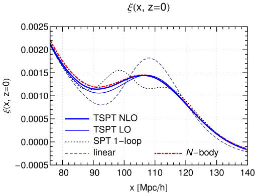
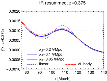
Our numerical results for the matter correlation function at redshift are summarized in Fig. 1, where we compare the TSPT results at LO and NLO with -body data, and also show the naive SPT 1-loop result for comparison. It is worth noting that the results are obtained from first principles without adjusting any free parameters. We further find that the difference between the NLO correlation function computed in TSPT and that obtained within the Zel’dovich approximation is about 5% in the region of the BAO peak (see Sec. 7.3). While small, this difference is above the estimated uncertainty in the TSPT calculation and the expected ultimate precision required to analyze the data of future surveys. Importantly, the TSPT framework can be systematically extended to take into account the next-order contributions, as well as the corrections due to the short-distance dynamics.
The paper is organized as follows. In Sec. 2 we outline the basic formalism. In Sec. 3 we describe how to identify the enhanced IR-effects and establish the power counting rules. The resummation of LO contributions is performed in Sec. 4 for the power spectrum and bispectrum. In Sec. 5 we extend the resummation to diagrams with loops of short modes. Next-to-leading IR contributions are resummed in Sec. 6 and a concise formula for the resummed correlation functions is derived. In Sec. 7 we discuss the practical implementation of our procedure, compare our result to -body data and discuss the BAO shift. Section 8 is devoted to conclusions and discussion of future directions. Appendices A—E contain details of the calculations, whereas in Appendices F, G we present an alternative derivation of IR resummation of the power spectrum in SPT and compare our results with the exact formulas in the Zel’dovich approximation.
2 TSPT and wiggly-smooth decomposition
In this section we first briefly remind the basic elements of the TSPT approach to large-scale structure formation (see [24] for a detailed presentation) and then discuss our strategy to identify IR enhanced effects on the BAO peak by decomposing the matter power spectrum as well as the TSPT vertices into smooth and oscillatory components.
2.1 Brief review of TSPT
We are interested in the time evolution of correlation functions of the overdensity field and the velocity divergence field , whose time-evolution is governed by the continuity and Euler equations for the peculiar flow velocity ,
| (2.1a) | |||
| (2.1b) | |||
where and . Here is conformal time and is the matter density fraction. It is well-known [7] that in the case of an Einstein–de Sitter universe these equations can be cast in a form free from any explicit time dependence by introducing the time parameter , where is the linear growth factor, and appropriately rescaling the velocity divergence
| (2.2) |
with . For the realistic CDM cosmology, the above substitution leaves a mild residual time dependence which, however, has little effect on the dynamics. Following conventional practice we will neglect this explicit time dependence in the equations, although none of our findings crucially depend on this restriction. With a slight abuse of language we will refer to this setup as ‘exact dynamics’ (ED). For comparison, we also consider Zel’dovich approximation (ZA) obtained by replacing the Poisson equation by . The linear growth factor plays the role of the expansion parameter in TSPT. In order to emphasize this, and in analogy to notation used in quantum field theory, we denote it by
| (2.3) |
We also use the short-hand notation , and analogously for .
The main idea of the TSPT approach is to substitute the time evolution of the overdensity and velocity divergence fields, and , by that of the their time dependent probability distribution functional. For adiabatic initial conditions only one of the two fields is statistically independent. We choose it to be the velocity divergence field , and its distribution functional is denoted by . At any moment in time, the field can be expressed in terms of as
| (2.4) |
where the kernels can be found in Appendix A and we introduced the notation .
Equal-time correlation functions for or can be obtained by taking functional derivatives with respect to the external sources or , respectively, of the following generating functional,
| (2.5) |
For example, the matter power spectrum is given by
| (2.6) |
It is useful to expand as a series in powers of ,
| (2.7) |
where is a normalization factor. The vertices have the physical meaning of 1-particle irreducible contributions to the tree-level correlators with amputated external propagators, and are counterterms, whose role is to cancel divergences in the loop corrections [24]. Both satisfy a hierarchy of equations which replace the dynamical equations of SPT. For the purposes of this paper the expressions for will not be needed. In the case of Gaussian initial conditions, the vertices have universal dependence on time both in ZA and ED,
| (2.8) |
where the TSPT coupling constant is defined by (2.3) and are time - independent functions generated by recursion relations given in Appendix A. Due to momentum conservation, the latter are proportional to a -function of the sum of their arguments; in what follows we use primes to denote the quantities stripped off such -functions,
| (2.9) |
The Gaussian part of the integral (2.5)
| (2.10) |
is the seed in the recursion relations (A.4b), (A.5b) so the vertices can be seen as functionals of the initial power spectrum .
The TSPT perturbative expansion is organized by expanding the generating functional (2.5) over the Gaussian part of , which is equivalent to an expansion in the coupling constant . This calculation can be represented as a sum of Feynman diagrams, whose first elements are summarized in Fig. 2: is represented by a line (propagator), the different elements (with ) and correspond to vertices, and are depicted as vertices with an extra arrow. To compute an -point correlation function of the velocity divergence one needs to draw all diagrams with external legs. For the correlators of the density field one has to add diagrams with external arrows.
2.2 TSPT in terms of wiggly and smooth elements
The initial power spectrum that sources the different elements of TSPT can be decomposed into a smooth part (with the maximum at corresponding to the matter-radiation equality) and an oscillatory part (or wiggly power spectrum) that describes the impact of the BAO,
| (2.11) |
Here we have factored out the time-dependence given by the growth factor and introduced a book-keeping parameter to count the powers of in various expressions. As for the vertices, the bar denotes the time-independent power spectra. The amplitude of the wiggly power spectrum is suppressed compared to that of the smooth power spectrum in a realistic cosmological model. Its value can be estimated as [26] (see also [27]),
| (2.12) |
The wiggly power spectrum can be parametrized as [27, 26],
| (2.13) |
where , the Silk damping scale is and is the dark matter transfer function which is slowly varying555It tends to 1 at and behaves as at higher . with . For our numerical analysis we do not use (2.13), but extract the wiggly part by fitting a smooth multi-parameter template to the linear power spectrum for a given cosmological model. The details of this procedure are outlined in Appendix B. The corresponding (time-independent) ratio is shown by the solid curve in Fig. 3 for the case of the reference cosmological model used later on. Notice that this ratio vanishes both at low and high wavenumbers.
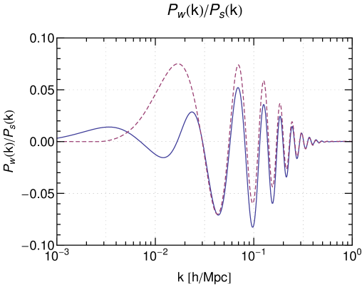
To check that the results do not depend on the precise prescription for separating the total power spectrum into smooth and wiggly components, we have also used an alternative decomposition (see Appendix B) with depicted by the dashed curve in Fig. 3. We find that the difference in the final results for the total power spectrum and the correlation function obtained using the two forms of are at the sub-percent level, below the uncertainties introduced by other approximations. This is to be expected: the ambiguity in the wiggly-smooth decomposition is relevant at large scales, , which are essentially unaffected by the non-linear IR dynamics. As will become clear later, in the physical observables at these scales the smooth and wiggly components are simply summed back, and the ambiguity disappears. Similarly, an overall vertical off-set between the two curves in Fig. 3 at does not contribute into the BAO feature.
The decomposition (2.11) can be extended to all the vertices, since they are functionals of the initial power spectrum. Let us start with from (2.10),
| (2.14) |
Given that the vertex generates all the higher vertices by the recursion relation (A.5b), one can introduce a similar decomposition for all the vertices
| (2.15) |
The vertices are computed using as an input in (A.5b).
The decomposition (2.15) can be introduced back in the partition function (2.7). Since the and kernels are not functionals of the linear power spectrum [24] (see also Appendix A), they are not subject to the wiggly-smooth decomposition. The leading order corresponds to the smooth correlation functions. The results include the wiggly contribution. In terms of diagrams, they can be summarized in the form of a new wiggly propagator (represented by a wiggly line) and by wiggly vertices (represented by a dashed circle), see Fig. 4. We use small dots to depict the smooth vertices and straight lines to represent the smooth power spectrum. The terms are quadratic in and will be neglected.
The graphs with the wiggly elements are loosely referred to as wiggly graphs. For instance, the tree-level wiggly bispectrum is given by the following four wiggly graphs666 In terms of SPT kernels the result of (2.17) can be rewritten as (2.16) ,
| (2.17) | ||||
To obtain the matter density bispectrum one has to add to the previous expression six more graphs with the vertex ,
| (2.18) | ||||
In what follows we set whenever there is no possible confusion.
3 IR enhanced diagrams and power counting
One of the advantages of the TSPT approach is that all of its building blocks are free of spurious infrared enhancements. In particular, the vertices are finite in the limit , where is any subset of the arguments of [24]. In contrast, within SPT individual vertices have poles in which cancel only after summing all contributions at a given order. Nevertheless, as mentioned previously, for a linear power spectrum with an oscillatory behavior the cancellation of enhanced terms is incomplete for . In this section we show how to extract these enhanced contributions within TSPT and then discuss power counting rules. These are helpful to organize the resummation of enhanced contributions, and later on to develop a perturbative expansion for taking sub-leading corrections to the resummed result into account.
3.1 IR enhanced vertices
We consider a TSPT -point vertex evaluated with arguments that have magnitudes given schematically by two different scales: a hard scale denoted by and a soft scale denoted by , with
| (3.1) |
Let us first analyze the three-point vertex . Using (A.4b) or (A.5b) we find,
| (3.2) |
where is given in (A.6). In the limit (3.1) the rightmost term in (3.2) is smaller than and will be neglected in what follows. The other terms provide an expression of the form
| (3.3) |
where we have used that the derivatives of the smooth component scale as and expanded . In contrast, we kept the finite difference for the wiggly component that varies substantially for .
It is convenient to use compact notations by introducing the linear operator
| (3.4) |
This operator will play a central role in the following, and therefore we elaborate on some of its properties. Consider first its action on a purely oscillatory function , where we are interested in the case . Expanding the exponent in the small parameter we obtain,
| (3.5) |
where we introduced . For the expression in the brackets is of order one, whereas the prefactor is enhanced by . On the other hand, if , Eq. (3.5) reduces to
| (3.6) |
so that the enhancement is given by . In a more realistic case the wiggly power spectrum can be viewed as an oscillating function that is modulated by a smooth envelope, c.c. with777Strictly speaking, due to existence of the Silk damping, . However, we use the simpler estimate from above since in practice we do not consider values of that are parametrically larger than . . For example, the parametrization (2.13) is of this form. Inserting this parameterization into (3.4) one observes that the derivatives acting on the envelope are suppressed compared to those acting on the oscillating part. They must be taken into account only when looking at the sub-leading corrections. We conclude that
| (3.7) |
where we introduced the small parameter
| (3.8) |
As we are going to see shortly, the enhancement by is the reason why the naive SPT loop expansion breaks down for the BAO. The sub-leading corrections coming from the derivatives of the envelope and higher terms in the expansion of the oscillating part correspond to contributions of order (or higher powers of ) that are suppressed relative to the leading enhancement. This will be important to establish systematic power counting rules.
It turns out to be useful to extend the action of to any wiggly element. This is done by recalling that the latter are linear expressions in with smooth -dependent coefficients. Then, by definition, acts on any occurrence of according to (3.4), leaving the smooth coefficients intact. For example,
| (3.9) |
and similarly for other . Note that an immediate consequence of this definition is that commutes with itself,
| (3.10) |
The result (3.3) for the 3-point vertex can be generalized by induction to arbitrary -point vertices with hard wavenumbers and wavenumbers going uniformly to zero. In Appendix C we prove the following formula,
| (3.11) |
where due to momentum conservation. Note that the leading IR enhancement is equal to the number of soft arguments. The maximal enhancement happens for the case of soft wavenumbers where we have
| (3.12) |
which scales as . Clearly, the sensitivity of the vertices to the large parameter grows with . In the subsequent sections we show how these large enhancement factors can be resummed within a systematic approach.
3.2 Leading diagrams and power counting rules
Consider a loop diagram containing a wiggly TSPT vertex with external legs and legs attached to the loops. As we saw above, this vertex is enhanced by powers in the limit where its arguments flowing in the loops become soft compared to the external wavenumbers . In order to extract the corresponding enhancement of the loop diagrams, we split all loop integrations into a soft part with and a hard part with . The scale is in principle arbitrary, and observables do not depend on it when computed exactly. Nevertheless, this splitting allows us to separately treat the IR and UV parts of loop integrations, and resum the large IR loops. Any residual dependence on should be taken as an estimate of the theoretical uncertainty, that should become smaller and smaller when computing at higher orders. In practice, the BAO feature is mostly affected by the modes with between and , so the range can be expected to lead to good convergence properties. We will return to the choice of in Sec. 7.
To account for the IR enhancement, we identify the expansion parameter with (cf. (3.8))
| (3.13) |
where is the characteristic scale giving the dominant contributions into the IR loop integrals. As will become clear below by inspection of the eventual expressions (3.24), (7.2) for the IR enhanced loops, the integrand in them peaks roughly at the maximum of the smooth power spectrum implying .
In addition to , the relevant parameter that controls the loop expansion is given by the variance of the input linear power spectrum. The latter is dominated by the smooth component . Due to the splitting into an IR (‘soft’) and UV (‘hard’) parts we can discriminate two variances
| (3.14) |
For example, for a realistic CDM model one has (recall that ) for the choice Mpc, whereas is formally UV divergent. In practice, the hard part of the loop corrections remains finite due to additional suppression of the actual integrands in the UV. Still, these corrections are UV dominated and their reliable calculation requires proper renormalization of the contribution due to very short modes. On the other hand, while the importance of the UV counterterms increases for high wavenumbers and at higher orders of the perturbation theory, they are not essential for the calculation of hard one-loop corrections to the power spectrum at the BAO performed in this paper. The latter corrections are well-behaved and are of order few at . We postpone the study of the UV counterterms in TSPT for future work and focus in this paper on the IR loops. will be used in what follows as a formal counting parameter for the number of hard loops.
Although seems to be rather small, we will now argue that soft loops are enhanced by a factor for the wiggly observables. Therefore they are proportional to the product which is at low redshift, implying that the corresponding soft loops need to be resummed. Consider, for example, 1-loop corrections to the wiggly power spectrum, given by the following TSPT diagrams,
| (3.19) | ||||
| (3.22) |
The loop integration in each diagram can be either hard, , in which case the diagrams are counted at order , or soft, , and are of order . Only the soft contributions can be IR enhanced, so we focus on them for the moment. The diagrams in the first line of (3.22) are never IR-enhanced, i.e. they are at most of order , because they do not contain a wiggly vertex. On the other hand, the diagrams with the wiggly vertices do receive an IR enhancement. The first diagram in the second line contains and is according to (3.12), (3.7) of order . The last diagram contains , and using (3.12), (3.7) we find that it is of order and thus is the most IR-enhanced one-loop diagram. At leading order in it is given by
| (3.23) |
where in the last step we defined the operator which can be written as
| (3.24) |
In terms of our power counting
| (3.25) |
As discussed previously, the product can be of at low redshift and therefore this one-loop contribution can be comparable to the linear wiggly spectrum.
In order to identify and eventually resum such terms we now discuss how to determine the order of an arbitrary -loop diagram in our power counting. This is valid for any -point correlation function, with external wavenumbers around the BAO scale, . Given a TSPT diagram with loops (i.e. scaling as ), one must
-
1.
choose for each propagator and each vertex whether it is smooth or wiggly. Since we are interested in diagrams that contain one power of , at most one element (either propagator or vertex) can be wiggly. To obtain the full answer, one eventually needs to sum over all possibilities to choose a vertex or propagator to be the wiggly one.
-
2.
assign each loop to be either hard () or soft (). Formally, this can be done by splitting the linear input spectrum into two parts as , and calling a loop hard if all propagators and vertices along the loop contain only power spectra of the former type888 Strictly speaking, the splitting into hard and soft contributions is only necessary for the loops that contain a wiggly vertex. For other loops, since in a realistic case, it is effectively irrelevant whether we make this split or not.. The number of hard loops is denoted by and the number of soft loops by . Trivially , and the diagram contributes at order . Again, to obtain the full answer, one needs to sum over all assignments eventually.
-
3.
count the number of soft lines that are attached to the wiggly vertex. We call this number . According to (3.12), the IR-enhancement is .
The order in our power counting of a contribution characterized by the numbers is therefore given by999To be more precise, this provides an upper estimate for the magnitude of the contribution. Specific terms can be further suppressed, as will be seen below.
| (3.26) |
If a diagram contains no wiggly vertex then and no IR-enhancement occurs. The most IR-enhanced contributions have the largest value of . As a single loop cannot contain more than two lines attached to the same vertex, we have the inequality . This means that the most IR enhanced contributions are of order . As argued before is at low redshift and therefore it is desirable to resum all diagrams with the maximal enhancement . This is the subject of the next section.
4 Resummation of leading infrared effects
Here we perform the resummation of dominant IR enhanced diagrams contributing into wiggly observables. We start with the power spectrum, then consider the bispectrum and outline the generalization to higher -point functions. We work at the order , i.e. neglecting the hard loop corrections. The task of taking them into account is postponed till Sec. 5.
4.1 Power spectrum
The most IR-enhanced contributions correspond to diagrams with and , i.e. all loops are soft and they contain a wiggly vertex to which soft lines are attached. At one-loop, the most IR enhanced diagram is the tadpole diagram (3.23) with soft loop and soft lines attached to (the two lines that belong to the loop). At two-loop, , the most IR-enhanced diagram should contain a wiggly vertex with soft lines attached to it. In addition, the IR enhancement can only occur if also a hard momentum flows through the wiggly vertex. For this can only be the external momentum. Therefore, the most IR-enhanced diagram has to contain a wiggly vertex with four soft arguments attached to loops and two hard arguments that correspond to the two external legs. The only possibility that remains is a single diagram, given by a double-tadpole. Analogously, at higher loop orders, the most IR-enhanced diagrams are obtained by attaching more and more loops to the wiggly vertex in the center. The first few diagrams that contribute to the wiggly part of the power spectrum are shown in Eq. (1.4). It is natural to call them daisy diagrams. Note that the leading IR-enhanced contributions are the same for the density and velocity power spectra. Indeed, within TSPT the power spectrum is obtained from that of by adding diagrams with the kernels (see Sec. 2.1). These kernels do not depend on the wiggly power spectrum and are therefore not subject to IR enhancement. Consequently, diagrams involving kernels give subdominant contributions at each loop order.
The daisy diagram with loops, all of which are soft (i.e. ), is given by
| (4.1) |
The symmetry factor in this formula arises as follows: there are ways to choose the two external legs, and ways to connect all the remaining lines into the loops. Making use of (3.12), one obtains
| (4.2) |
where the operator has been defined in (3.23). The sum over all daisy graphs gives the leading-order IR-resummed wiggly power spectrum
| (4.3) |
We see that the operator exponentiates.
The total power spectrum is obtained by adding the smooth part which, to the required order of accuracy, can be taken at tree level. This yields,
| (4.4) |
Let us stress again that this expression holds both for the density and velocity divergence power spectra. Moreover, it is the same in ED and ZA as the expansion (3.12) used in the derivation is valid in both cases. The difference between ED and ZA and between and appears for higher correlators and for the power spectrum beyond the leading order.
4.2 Bispectrum and other -point correlation functions
In this section we extend the resummation procedure of the IR-enhanced loop contributions to the wiggly part of higher order correlation functions. We first discuss the bispectrum and then general -point correlation functions.
The wiggly part of the tree-level bispectrum for the velocity divergence field is given by the four graphs (2.17), whereas for the density bispectrum one has to add the graphs (2.18). At one loop order, and assuming all external wavenumbers are hard, the most IR-enhanced contributions are obtained by ‘dressing’ the wiggly vertices and propagators in (2.17), (2.18) with a soft loop () attached to the wiggly vertex,
| (4.5) | ||||
| (4.9) |
Within our power counting, these diagrams contribute at order compared to the tree-level bispectrum. Using a similar reasoning as for the power spectrum, one finds that at higher loop orders the most IR-enhanced corrections are given by daisy diagrams obtained by attaching more soft loops to the wiggly vertices appearing in each diagram in (4.5). Parametrically, these -loop diagrams scale as
| (4.10) |
and thus need to be resummed.
The daisy diagrams centered on the propagator (like the second and third terms in (4.5)) are essentially the same as those appearing in the calculation of the power spectrum from the previous subsection. They are evaluated using Eq. (LABEL:leadlooplim) and their resummation leads to the replacement of the external wiggly propagators in the tree level expression,
| (4.11) |
A new type of contributions comes from one-particle-irreducible (1PI) diagrams with soft loops dressing the 3-point vertex (like the first diagram in (4.5)). In view of future uses, let us consider the general case of a wiggly vertex with hard wavenumbers dressed by soft loops,
| (4.12) |
Using Eq. (3.11) we obtain for the leading IR-enhanced part,
| (4.13) |
Clearly, resummation of these diagrams results in the substitution of the wiggly vertex,
| (4.14) |
Combining all terms together, one obtains the resummed bispectrum,
| (4.15) |
Recall that in the last expression the operator should be understood as acting on every occurrence of in the tree-level expression for the bispectrum. In terms of the SPT kernels, Eq. (4.15) can be rearranged into a somewhat simpler form,
| (4.16) |
The total bispectrum is obtained by adding to this expression the smooth tree-level part.
The above result extends to any equal-time -point correlation functions of or with hard external legs. Namely, the IR resummation at LO amounts to simply substituting the wiggly part of the linear spectrum, , that enters via wiggly vertices and propagators within the TSPT tree-level calculation, by the resummed expression . This can be summarized in the following compact form,
| (4.17) |
where is understood as a functional of the linear power spectrum. Note that, since the tree-level -point correlation functions, when summed over all perturbative contributions, coincide in SPT and in TSPT, one can equivalently use the replacement (4.11) in the usual SPT computations. However, the clear diagrammatic representation as daisy resummation is only possible within TSPT. In addition, TSPT allows to systematically compute corrections to the LO resummation presented above.
5 Taking into account hard loops
So far, we have considered and resummed the contributions that in the power-counting scheme of Sec. 3.2 are of order . We now discuss corrections to this result. One can discriminate two types of corrections:
- (1)
-
(2)
Diagrams with one hard loop, , and otherwise maximal IR enhancement . These diagrams are suppressed by one factor of relative to the leading order.
We refer to these two types of contributions as NLOs and NLOh, respectively. When combined, they constitute the total NLO correction. In this section we analyze the contributions of the second type, while NLOs corrections will be included in the next section.
We start from the ‘hard’ 1-loop contribution to the wiggly matter power spectrum101010For the power spectrum one simply omits the diagrams containing the kernels .,
| (5.4) | ||||
| (5.7) | ||||
| (5.10) | ||||
| (5.14) | ||||
| (5.18) |
where the wavenumber running in the loop is taken to be above the separation scale , . Note the appearance of a diagram with the counterterm in the second line. Similarly to the case of the tree-level bispectrum, all wiggly elements in these graphs can be dressed with soft daisies producing contributions of order
| (5.19) |
Resummation of these contributions proceeds in a straightforward manner using the general expressions (4.12), (4.13) and yields,
| (5.20) |
where the r.h.s stands for the 1-loop diagrams (5.18) computed using the wiggly power spectrum instead of the linear power spectrum as an input.
Two comments are in order. First, the diagrams in the third and fourth lines in (5.18), as well as their descendants obtained by dressing with daisies, contain a wiggly element inside the loop. This implies that the integrand of the corresponding loop integral is oscillating leading to cancellation between positive and negative contributions. As a result, the corresponding diagrams are further suppressed compared to the naive estimate (5.19). In fact, the suppression is formally exponential, as follows from the general formula for the Fourier transform of a smooth function,
From the viewpoint of our power-counting scheme, these contributions are ‘non-perturbative’ and can be included or neglected without changing the accuracy of the perturbative calculation. We prefer to keep them as it allows us to write the result of the IR resummation in the compact form (5.20).
Second, an alert reader might have noticed that the contributions discussed so far, namely those obtained by the daisy dressing of (5.18), do not exhaust all possible diagrams that formally would be of order (5.19) by the power-counting rules of Sec. 3.2. The remaining diagrams fall into two categories. First, there are diagrams where a hard line closes on a wiggly vertex, which is in its turn attached to the external legs via a soft loop; a two-loop example is given by
| (5.22) |
However, these diagrams necessarily contain a wiggly vertex inside a hard loop and thus, according to the previous discussion, are exponentially suppressed. They can be safely neglected. Another set of extra diagrams is given by the graphs where a hard loop is attached to a smooth propagator that belongs itself to a soft loop. For example, at two-loop order these are
| (5.24) | ||||
The subdiagrams attached to the soft loop combine into the hard part of the one-loop correction to the smooth velocity divergence power spectrum , see [24]. As before, the ‘hard part’ means that the loop integration in is restricted to . This correction could be viewed as a loop-correction to the operator suggesting to substitute the smooth power spectrum in by . While it is tempting to do this replacement, we refrain from this step for two reasons. First, this would correspond to a partial resummation of hard loops, and therefore goes against the rigorous expansion in our power counting parameters. Second, and more importantly, the hard loop corrections to the power spectrum are universally suppressed as at soft momenta due to the well-known decoupling of long and short modes [28, 29] (see also [30]). This suppression essentially removes the IR enhancement of the operator in (5.24), so that the term (5.24) is suppressed by compared to the contributions resummed in (5.20). Here is the characteristic IR scale which, as discussed in Sec. 3.2, is of order . Therefore, the contribution (5.24) is small as long as . In the real universe the hierarchy between and cannot be too large. Nevertheless, we have checked numerically that for the standard CDM and the realistic range of values Mpc, the contribution (5.24) is quantitatively unimportant. In what follows we neglect the diagrams with hard loops inside soft ones.
The expression (5.20) can be cast in a more convenient form by the following steps. Let us add and subtract the soft part of the one-loop diagrams,
| (5.25) |
where in the last line stands for the total one-loop correction and we used Eq. (3.23) to express the leading soft-loop contribution. Combining this with the one-loop correction to the smooth power spectrum and the LO expression (4.4) we obtain the final expression for the power spectrum with NLOh corrections included,
| (5.26) |
Here is understood as the functional of the input linear power spectrum; the latter has been modified by the IR resummation. Note the appearance of the term in the ‘tree-level’ part of the expression (5.26) that is important to avoid double counting of the soft contributions.
The formula (5.26) can be straightforwardly generalized to other -point functions, both of density and velocity divergence. We give here the final result without derivation,
| (5.27) |
Moreover, it is possible to include higher hard loops, i.e. corrections of order with . Let us do it for the power spectrum111111The derivation does not depend on the type of the power spectrum (, or ) so we do not specify it explicitly.. Repeating the arguments that led to Eq. (5.20), one finds at the NNLOh order,
| (5.28) |
where the 2-loop contribution on the r.h.s. is ‘double-hard’, i.e. the integration in both loops run over . This is equivalently written in the form,
| (5.29) |
where the first term contains the total 2-loop contribution, whereas the second and third terms are ‘hard-soft’ and ‘soft-soft’ respectively. Next, we use the relations valid at the leading soft order,
| (5.30a) | ||||
| (5.30b) | ||||
where to obtain the last expression in (5.30b) we have again added and subtracted the soft one-loop contribution. Combining everything together and with the NLOh expression (5.26) we arrive at a compact formula,
| (5.31) |
Its extension to other correlation functions and to higher orders in hard loops can be done by proceeding analogously.
The expressions (5.26), (5.27), (5.31) do not take into account subleading soft corrections. These are formally of order and thus can be expected to be significant as in the real universe the latter parameter is not small, . Therefore the next section is devoted to a detailed computation of these corrections. Notably, we will find that the dominant NLOs corrections are already captured by the one-loop term in (5.26) for the power spectrum, such that it works remarkably well. Still, it is important to properly assess the NLOs contributions because they are required for a reliable determination of the shift of the BAO peak, as discussed in Sec. 7.4.
6 Resummation of infrared effects at next-to leading order
Here we discuss corrections to the power spectrum that are suppressed by one power of relative to the leading order IR resummed results discussed previously. There are two possibilities to obtain such corrections: () On the one hand, one can consider the same daisy diagrams, i.e. with maximal IR enhancement , but take into account the first sub-leading correction in the expansion of the wiggly vertex (3.12). () On the other hand, one can consider new diagrams with . All diagrams that contribute at to the velocity divergence power spectrum at increasing number of loops are given by
| (6.1) |
Here all loops are soft, i.e. integrated over wavenumbers below . The daisy diagrams containing the vertices at 1, 2, 3-loop, and so on, belong to the category (). The diagrams containing at 1, 2, 3-loop, and so on, have , and therefore belong to category (). All diagrams in category () are related to two new diagrams: the fish (last diagram in the first line) and oyster (last diagram in the second line). All higher-loop diagrams of type () are obtained by dressing the wiggly vertex contained in these diagrams with daisy loops, such as e.g. the middle diagram in the second line and the last two diagrams in the last line. The matter power spectrum includes in addition at the dressed fish diagram with the vertex ,
| (6.2) |
We first consider the diagrams of type (b). Dressing of the fish diagrams simply leads to the already familiar replacement (4.11). We do not need these contributions explicitly, as our eventual goal is to combine them with the hard corrections (5.20) to form the total fish diagrams evaluated using the modified wiggly power spectrum (4.11).
For the oyster diagram, a straightforward evaluation using the expansion (3.11) for and the exact expression for yields,
| (6.3) |
where we introduced the operators,
| (6.4a) | ||||
| (6.4b) | ||||
and () in ED (ZA). The dressing of the wiggly vertex by daisies again leads to the replacement (4.11) in this formula,
| (6.5) |
Next, we turn to the contributions of type (a), i.e. daisy diagrams expanded to the NLOs order. Remarkably, these also can be resummed. To see this, we need the first corrections in to Eq. (3.12). The latter are derived in Appendix C with the result,
| (6.6) |
where and are new finite-difference operators acting on that are defined in (C.12) and (C.15). Inserting this expression into Eq. (LABEL:leadlooplim) and summing over the number of loops we obtain,
| (6.7) |
where
| (6.8) |
and we used the relation
| (6.9) |
It is desirable to connect the expression (6.7) to the one-loop daisy graph computed using the modified linear power spectrum,
| (6.10) |
One may be tempted to compute this by simply making the replacement (4.11) in the NLO expression (C.14) for the vertex function . However, this would produce a mistake at the NLOs order. The reason is that the operator depends on the hard wavenumber (see Eq. (3.24)). When is evaluated with the new wiggly power spectrum , the operator gets shifted,
The correct expression for the vertex taking this shift into account is derived in Appendix C, see Eq. (C.23). Using it to evaluate the loop we obtain,
| (6.11) |
This should be compared with (6.7). We have
| (6.12) |
Notice that the operators , have dropped out of this relation.
We are now ready to combine all NLO contributions together. These include the resummed hard loops (5.20), soft fish diagrams, the contribution of the soft oyster diagram (6.5), and the resummed daisies (6.12). Adding to them the smooth part we obtain,
| (6.13) |
This is our final result for the full NLO power spectrum. At face value, it differs from the NLOh formula (5.26) only by the last term. However, we emphasize that now all subleading IR corrections have been consistently included. In particular, the one-loop contribution differs for ZA and ED as well as for density and velocity correlators at the NLOs order. The last term scales as compared to the leading piece. This reflects that it receives contributions only starting from 2-loops. Nevertheless, this term is of order in our power counting and therefore must be retained. Still, we will find below that it happens to be numerically small.
7 Practical implementation and comparison with other methods
In this section we first discuss how the IR resummed power spectrum obtained in TSPT can be evaluated in practice, and then compare to other analytical approaches as well as to -body data. In the last part we discuss the predictions for the shift of the BAO peak.
7.1 Evaluation of IR resummed power spectrum
After decomposing the linear power spectrum into smooth and oscillating (wiggly) contributions121212 In this section we adopt the conventional notations and denote the growth factor and the linear power spectra at simply by ., we need to evaluate the derivative operator defined in (3.24), that describes the IR enhancement. This is done using
where is the small expansion parameter related to IR enhancement defined in (3.8) and . Recall that Mpc) is the scale setting the period of the BAO oscillations. A straightforward computation yields
| (7.1) |
with
| (7.2) |
where are spherical Bessel functions and is the (a priori arbitrary) separation scale of long and short modes, that has been introduced in order to treat the perturbative expansion in the two regimes separately. Since the exact result for the power spectrum and other observables is independent of , any residual dependence on it can be taken as an estimate of the perturbative uncertainty. The IR resummed power spectrum at leading order following from (4.4) is given by
| (7.3) |
where the first term corresponds to the smooth part of the linear spectrum. The leading effect of IR enhanced loop contributions is an exponential damping of the oscillatory part of the spectrum.
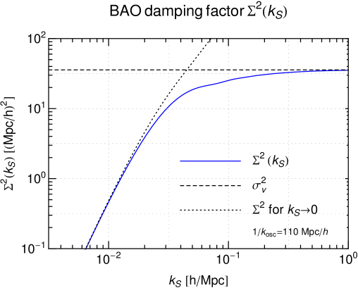
Let us now discuss the choice of . By inspection of the integrand in (7.2) we find that it peaks at Mpc, but gives significant contribution into the integral up to wavenumbers Mpc. This is corroborated by the numerical evaluation of the damping factor as a function of ; the result is shown in Fig. 5 for a realistic CDM model. For very small values of the IR separation scale it approaches the limiting form , while for large it asymptotes to a constant . It is desirable to take as large as possible to include more IR contributions and minimize the dependence of the damping factor on . On the other hand, cannot be taken too large as the previous analysis relies on the IR expansions which are valid for . As a compromise, we consider several values of around the BAO scale Mpc. We are going to see that the dependence of our results on the precise choice of in this range is very mild.
At NLO, the IR resummed power spectrum (6.13) can be written in the form131313 Since we are keeping NLO terms, one should in principle keep also the first sub-leading corrections in the evaluation of the derivative operator in (7.1). However, it turns out that this correction cancels in (7.4) at NLO precision. The simplest way to see this is to go back to Eqs. (6.7), (6.11) and substitute in them the expansion (7.1) keeping track of the terms. By comparing the resulting expressions one finds that the relation (6.12) holds with NLO precision if is everywhere replaced by . As all other contributions comprising (6.13) do not contain an part, the replacement in them is also justified leading to (7.4).
| (7.4) |
where in ED ( in ZA). The first term in the second line of (7.4) corresponds to the standard one-loop result, but computed with the LO IR resummed power spectrum, instead of the linear one. As was demonstrated in [24], the sum over all one-loop diagrams in TSPT agrees with the SPT result. Therefore, in practice, one can use the usual expression , however evaluating the loop integrals and with the input spectrum (7.3) instead of the linear spectrum.
Finally, the finite-difference operators in the last term can be evaluated similarly to . After somewhat lengthy but straightforward calculation, we obtain
| (7.5a) | ||||
| (7.5b) | ||||
with
| (7.6) |
The functions are given in App. D. The result (7.4) is valid for both density, velocity and cross power spectra when using the appropriate expressions for the one-loop correction. In addition, one can obtain the result in ZA by using the corresponding one-loop expression with kernels computed in ZA and setting .
7.2 Comparison with other approaches
Let us now compare our results to other approaches existing in the literature. From a phenomenological viewpoint, it is well-known that an exponential damping factor applied to the oscillating component of the power spectrum gives a reasonable description of the BAO peak in the measured two- and also three-point correlation functions, see e.g. [6] and references therein. Therefore, the aim of perturbative descriptions is to derive this behavior from first principles, identify effects that go beyond a simple damping, and give a definite quantitative prediction as well as an estimate of the theoretical error.
There exist many schemes to derive non-linear corrections to the BAO peak within cosmological perturbation theory, here we focus on a few of them. In [9], the RPT formalism [31] was used to obtain a formula of the form.
| (7.8) |
where is the propagator and is the part due to the mode coupling. The propagator describes how a perturbation evolves over time and is not a Galilean invariant quantity. As such, it contains IR enhanced contributions corresponding to the translation of inhomogeneities by large-scale flows. When resummed at the leading order, these contributions produce an exponential damping factor at high ,
| (7.9) |
with , and being a UV cut-off of the theory (). In the RPT-based approach this form of the propagator is substituted into (7.8). A similar result is derived in the Lagrangian picture in [22, 20]. Notice that the exponential damping in this case applies to the whole linear power spectrum, including both wiggly and smooth parts. Further developments of this idea have been proposed in [34].
While being successful on a phenomenological level, this approach is quite different from ours. In RPT, there is no clear parametric dependence that would single out the resummed set of contributions. In particular, for a smooth power spectrum the contributions resummed in (7.9) are of the same order as those comprising , and actually cancel with them [14, 13, 16, 15, 12, 17] as required by the equivalence principle. On the other hand, our approach is based on well-defined power-counting rules formulated directly for the perturbative expansion of equal-time correlation functions. As a result, we obtain a damping only of the oscillating part of the power spectrum, in line with the expected cancellation of IR enhancement for the smooth part. Furthermore, the damping factor given by (7.2) has a different structure from (7.9). Although for the real universe their numerical values happen to be very close to each other, the situation would be different for a universe with more power in very soft modes with wavenumbers . Finally, when taking NLO corrections into account our result (7.4) cannot be described anymore by a simple exponential damping of the overall power spectrum or its wiggly part.
Ref. [8] proposed a description of the IR enhanced effects on the BAO peak motivated by consistency relations between the bispectrum and the power spectrum based on the equivalence principle. This approach is related to the earlier perturbative framework developed in [18]. At leading order, our result (7.3) coincides with the results of [8] when choosing . The agreement essentially extends to the corrections produced by hard loops (see Sec. 5). Subleading soft corrections were not considered in [8]. TSPT gives a simple diagrammatic description of IR enhancement and provides a tool to systematically derive, scrutinize and extend the results found in [8]. In particular, the subleading soft corrections computed in the present work and entering in (7.4) capture the shift of the BAO peak, as we will see below, and the power counting allows in principle to go beyond NLO in a systematic way. Furthermore, the IR resummation in TSPT readily generalizes beyond the power spectra and applies to any -point correlation functions.
7.3 Comparison with -body data
We consider a CDM model with cosmological parameters matching those of the Horizon simulation [25]. The linear power spectrum is obtained from the CLASS code [32] and decomposed into smooth and oscillating components as described in Sec. 2.2.
In the following we show results for the correlation function, because it exhibits a clear separation between the BAO peak and the small-distance part of the correlations, and allows to visualize the effects on the BAO feature in a transparent way. The matter correlation function is related to the power spectrum as
| (7.10) |
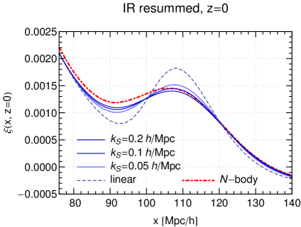
In Fig. 6, we show the leading-order IR resummed result for three different choices of (blue solid lines). The damping of the BAO oscillations described by corresponds to a broadening of the BAO peak in real space and gives already a relatively good description of the -body result shown by the red dashed line [25], especially when compared to the linear prediction (thin dashed line). Nevertheless, there are some differences, and the dependence on is not negligible.
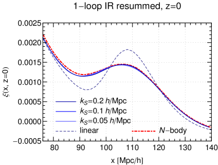
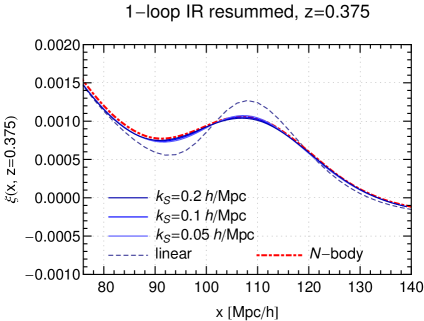
We now turn to the NLO result. The comparison of the matter correlation function obtained using (7.4) with the -body data is shown in Fig. 7. One observes that the agreement is considerably improved compared to the LO. Furthermore, the dependence on the separation scale is reduced. This is an important consistency check, because the dependence on vanishes in principle in the exact result. Thus, any residual dependence on can be taken as an estimate of the perturbative uncertainty, and it is reassuring that this uncertainty is reduced when going from LO to NLO.
We conclude that the systematic IR resummation gives a very accurate description of the correlation function at BAO scales. The residual discrepancies at shorter distances visible in Fig. 7 are expected due to several effects. The variance due to the finite boxsize, and the finite resolution of the -body data leads to an uncertainty of several percent141414Ref. [25] does not give error bars for the simulation data points. An estimate of the statistical variance using the number of available modes in the simulation as well as the finite resolution suggests that the uncertainty is at the few percent level in the range of scales relevant for BAO. This level of accuracy is also consistent with the difference between the correlation function extracted from Horizon Run 2 (Gpc, ) versus Horizon Run 3 (Gpc, ) data presented in [25].. In addition, the correlation function is sensitive to the UV physics which has been left beyond the scope of our present study.
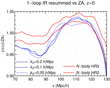
In Fig. 8 we show the ratio of the NLO result to the correlation function obtained in the Zel’dovich approximation151515Here by the Zel’dovich approximation we mean the leading order of Lagrangian perturbation theory. The 2-point correlation function in ZA was computed with the publicly available code ZelCa [35].. The differences are around in the BAO range, and therefore our results are broadly consistent with ZA, as expected. Nevertheless, the differences are larger than the ultimate precision that is desired to match future surveys. The ratio between the N-body correlation function and the one obtained in ZA is also shown on the same plot by the red line. The TSPT result agrees with the N-body data somewhat better than ZA in the BAO peak region, though the error range of the N-body data does not allow at the moment to clearly discriminate between the two. As discussed before, the TSPT framework can be systematically extended to NNLO, and further corrections from UV modes can be incorporated, which is left for future work.
Finally, we have compared the results for the correlation function computed using the full NLO formula (7.4) and its reduced version without the last term containing the operators , . The relative difference at does not exceed . Given the strong dependence of the omitted term on the growth factor and hence its quick decrease with redshift, one concludes that this term is negligible for all practical purposes.
7.4 Shift of the BAO peak
A valuable piece of information provided by the BAO peak is its position as a function of redshift that can be used as a standard ruler to infer cosmological parameters and probe possible alternatives to CDM (see [36] for a recent discussion in the context of modified gravity). The upcoming surveys aim at measuring this quantity with sub-percent accuracy [37]. Therefore, it is important to assess how non-linear dynamics offsets the BAO peak as compared to the linear prediction.
For concreteness we focus on the position of the maximum of the BAO peak which we denote by . There are two effects that contribute to its shift with respect to the linear result . First, the damping of the wiggly component in the power spectrum, which occurs already at leading order of the IR resummation, shifts the maximum because the correlation function is not symmetric. Second, at NLO the interactions of the modes in the BAO region with soft modes shift the phase of the BAO. This, in turn, translates into an additional shift of the peak in position space. Let us discuss these two contributions one by one.
It is convenient to decompose the correlation function into a smooth component and a component that describes the BAO peak,
| (7.11) |
that are inherited from the decomposition of the power spectrum into smooth and wiggly parts. In the region of the peak these two contributions are of the same order with being a factor of a few larger than . At the linear level, the condition for the maximum of the peak reads,
| (7.12) |
To obtain analytic estimates we represent the wiggly power spectrum as a product of the oscillating part and a smooth envelope (cf. Eq. (2.13)),
| (7.13) |
This implies that the position of the peak is close to . In what follows we seek the corrections to this relation. Writing
and treating the product as small we obtain from (7.12)
| (7.14) |
where we have neglected the integrals of rapidly oscillating functions. In particular, we have used the relation
If instead of the linear power spectrum, we consider the LO expression (7.3) with damped wiggly component, we obtain the position of the corresponding peak as
where is given by the expression (7.14), but with replaced by . One concludes that the shift of the LO peak relative to the linear one is
| (7.15) |
The two contributions in this formula are of the same order , where Mpc is the characteristic range of wavenumbers corresponding to BAO. At we have
| (7.16) |
We see that this LO shift is quite significant. It is worth emphasizing that it is exclusively due to the damping of BAO by large IR effects. The damping is the same in ED and ZA. Therefore is expected to be removed by the BAO reconstruction procedure which essentially uses the ZA to evolve the density field backward in time. To understand if this procedure can leave any residual shift we have to go to the next-to-leading order.
Writing the correlation function as one easily derives the additional shift of the peak induced by the second term,
| (7.17) |
One can check that the contribution of the smooth correlation function into this expression is negligible, so that one can safely replace in it .
We evaluate the LO and NLO contributions into the correlation function numerically using Eqs. (7.3), (7.4) for the power spectrum. The shift of the peak is then computed either directly by comparing the full correlation function to that at LO, or using (7.17). The results of this evaluation are presented in Table 1 (second and third columns). We consider three choices of the separation scale bounding the IR region.
| Mpc | |||
|---|---|---|---|
| Full | Eq. (7.17) | Eq. (7.22) | |
Modulo some scatter introduced by the dependence, our estimate for the NLO shift is around . This lies in the ballpark of the estimates obtained using different approaches [38, 9, 43, 42, 41] and agrees well with the value of the so-called ‘physical’ shift [38, 9] measured in the simulations [44, 39, 41]. While we expect that the NLO shift considered here agrees essentially with the ‘physical’ shift, the precise relation is not completely clear to us and we leave the task of understanding it for future work.
It is instructive to derive an analytic estimate for . It is shown in Appendix E that the NLO wiggly power spectrum has the form,
| (7.18) |
The first term in brackets receives contributions both from hard and soft modes, whereas the second term is exclusively due to soft modes with wavenumbers . It describes a phase shift of the wiggly component of the power spectrum. The precise form of the function is not relevant to us; it is only important that it depends smoothly on its argument. For we find,
| (7.19) |
where is defined in (7.5b). The other two coefficients are related to the density variance at the scale ,
| (7.20) |
where in the last formula Mpc is the Silk damping scale. The detailed expressions are given in Appendix E. It is worth to point out that the formula for is different in ED and ZA, as well as for the density and velocity divergence power spectra. Notice also the presence of the coefficient in (7.19) that discriminates between ZA () and ED ().
Next, we substitute (7.18) into (7.17) which yields,
| (7.21) |
Recalling the form (7.13) of one observes that the integral involving the first term in the numerator contains a rapidly oscillating function and thus gives a negligible contribution. In the second term we integrate by parts. Neglecting again integrals of rapidly oscillating functions and using (7.19) we arrive at
| (7.22) |
For realistic power spectra the ratio of integrals in the second term is of order at . It is worth noting that numerically the second term gives a subdominant contribution, so approximately one can write,
| (7.23) |
Still, we prefer to use the complete expression (7.22). Evaluating various contributions entering into it using the expressions from Appendix E and Eq. (7.5b) we obtain the estimates for the shift listed in the fourth column of Table 1. They are in reasonable agreement with the values obtained by the direct numerical evaluation of the correlation function.
As already mentioned before, the values of and are different in ED and ZA. Consequently, the BAO shift computed in ZA is somewhat lower than in ED:
depending on the choice of . Thus, while the ZA gives a rather accurate description of the BAO broadening, it underestimates the BAO shift. The difference is expected since the terms responsible for the BAO shift originate from the non-dipole parts of the interaction vertices, which are different in ZA and in ED. One concludes that, in principle, the BAO reconstruction based on ZA is expected to leave a small residual shift of order . However, this discrepancy is likely to be too small to have any significant effect on the determination of the BAO peak position.
Let us make a cautious remark. Although the above analysis provides a qualitative understanding of the origin of the BAO shift, as well as a trustable estimate of its order of magnitude, the concrete numbers listed in Table 1 should be taken with a grain of salt. They are smaller than the typical percent accuracy of our calculations, which calls for a re-assessment of various approximations made in their derivation. Also a realistic calculation of the BAO shift must include the effect of the bias [43, 42, 45]. We leave the study of these issues for future work.
Before closing this section, let us mention that the term proportional to in (7.19) generates also a distortion of the BAO peak that tends to make it more asymmetric. However, in CDM this effect is subdominant compared to the initial asymmetry of the peak present already at the linear level and amplified by various other terms in the NLO power spectrum. Still, the different contributions are not completely degenerate and it would be interesting to understand the impact of non-linear distortion on an accurate description of the BAO data.
8 Conclusions and outlook
In this work we have developed a systematic approach to describe the non-linear evolution of the feature imprinted in the matter correlation functions by baryon acoustic oscillations. We have provided a theoretical framework to efficiently resum corrections arising from non-linear interactions with long-wavelength modes that are particularly enhanced for the baryon acoustic feature.
Our approach is based on the framework of TSPT, that provides a perturbative description of structure formation manifestly free from spurious infrared divergences. Besides, it is based on an Eulerian description and therefore its practical implementation does not suffer from the complications arising in Lagrangian perturbation theory. These features make TSPT a convenient framework to discuss the effect of bulk flows on the BAO feature. We have first developed a formalism to isolate IR enhanced effects by splitting the TSPT propagators and vertices into smooth and oscillating (wiggly) contributions. Next, we identified the IR enhanced loop contributions, taking modes below an (a priori arbitrary) separation scale into account. These have a simple diagrammatic representation, with the dominant diagrams corresponding to daisy graphs. Finally, we have shown that within TSPT one can develop a modified perturbative expansion in which the large IR effects are resummed to all orders, and we computed next-to leading corrections including loops with hard wavenumbers as well as subleading contributions of the soft loops. Our leading IR resummed result agrees with that obtained in [8] using the symmetry arguments. TSPT provides a useful framework to systematically extend this result to higher -point functions and compute relevant corrections in a controlled way.
Our analysis provides a simple prescription for practical evaluation of the resummed correlation functions. At the leading order, it amounts to replacing the linear power spectrum in all calculations by the spectrum with damped wiggly component. This essentially remains true upon inclusion of hard loops, whereas the subleading soft loops introduce new terms. Our result for the IR resummed power spectrum with inclusion of all next-to-leading corrections is given in (7.4). It describes the non-linear evolution of the BAO peak with sub-percent accuracy, when compared to large-scale -body simulations. Although we found that the soft NLO corrections are rather small, they are important to capture the shift in the position of the peak maximum.
The residual dependence of our results on the artificial separation scale provides an estimate of the theoretical error, similar to analogous scale-dependencies in quantum field theory computations. At LO our result for the two-point correlation function close to the BAO peak exhibits a dependence on this scale at the level of several percent, when varying in the plausible range Mpc. As expected, the scale-dependence is reduced in the NLO result and is well below the percent level close to the BAO peak. The theoretical error estimated in this way is consistent with the agreement with -body data, except for short scales sensitive to the UV effects that were not considered in this paper.
Our results suggest several directions for future research. First, one can use the systematic TSPT approach to investigate the effects on the BAO peak in cosmological models beyond CDM. As examples we mention inclusion of neutrino masses or modifications of gravity. In particular, the NLO corrections affecting the BAO shift are sensitive to non-dipole corrections to the non-linear evolution that are not protected by the equivalence principle, and therefore can be particularly sensitive to modifications of the dynamics. Second, it will be very interesting to study in detail the BAO feature in the three-point function, as well as to extend the analysis to biased tracers. Finally, the TSPT framework can also be used to address the contributions of UV modes that influence correlation functions at shorter distances.
Acknowledments
We thank Stefano Anselmi, Tobias Baldauf, Martín Crocce, Guido D’Amico, Vincent Desjacques, Sergei Dubovsky, Mehrdad Mirbabayi, David Pirtskhalava, Francisco Prada, Roman Scoccimarro, Gabriele Trevisan, Fillippo Vernizzi, Matias Zaldarriaga and Miguel Zumalacárregui for helpful comments and discussions. We are grateful to Valery Rubakov for encouraging interest. S.S. acknowledges the hospitality of CCPP at NYU while this work was being finalized. D.B. and S.S. thank the Galileo Galilei Institute for Theoretical Physics for the hospitality and the INFN for partial support during the completion of this work. This work was supported in part by the Swiss National Science Foundation (M.I. and S.S.) and the RFBR grant 14-02-00894 (M.I.).
Appendix A Recursion relations for TSPT vertices
To define the building blocks of TSPT one starts with the non-linear SPT kernels,
| (A.1) |
These are used to write down the recursion relations for the vertices and [24]. The seeds for these relation are and given by Eq. (2.10). Higher vertices are different for ZA and ED. We have
| ZA: | (A.2) | |||
| ED: | (A.3) |
For the recursion relations read,
| ZA: | |||
| (A.4a) | |||
| (A.4b) | |||
and
| ED: | |||
| (A.5a) | |||
| (A.5b) | |||
where
| (A.6) |
The notation above means that the momentum is absent from the arguments of the corresponding function, and in the last lines of (A.5a), (A.5b) the summation is performed over all permutations of indices.
Appendix B Decomposition of smooth and wiggly components
In this appendix we describe our algorithms to separate the smooth and oscillating contributions to the matter power spectrum. In the first case, in order to obtain a smooth power spectrum we perform a fit to the linear power spectrum obtained with the CLASS code [32] that is inspired by the Eisenstein-Hu formula [33]. Specifically, we find that the smooth part can be well described by the parametric form
| (B.1) |
where the transfer function is parameterized as in [33],
| (B.2) |
Here we treat the coefficients and as free parameters that are determined by fitting to the linear power spectrum, see Tab. 2. In addition, we introduce a correction of the Eisenstein-Hu fitting formula to account for a slight residual offset at large given by
| (B.3) |
The values of we used are also given in Tab. 2. The oscillating component is then given by . It is plotted in Fig. 3 by the solid line.
Appendix C Asymptotic behavior of the vertices in the soft limit
In this Appendix we study in detail the form of the TSPT vertices with soft legs. First, we derive the leading order expression (3.11). Next, we extend the analysis to include the subleading corrections and obtain Eq. (6.6), as well as the expression for the four-point vertex evaluated on the modified linear power spectrum used in the derivation of Eq. (6.11).
C.1 vertices in the soft limit: leading order
We split the arguments of the vertices into ‘hard’ momenta , , , that are are fixed and ‘soft’ momenta , which are sent uniformly to zero,
| (C.1) |
To prove (3.11) we proceed by induction. Let us fix and assume that Eq. (3.11) has been already proved for all . Equation (3.11) holds trivially for . Now, suppose that it is valid for all such that . Our task is to show that it also holds for .
We focus on ED; the derivation for ZA can be recovered by simply ignoring all contributions due to the kernels. We will use the shorthand It is convenient to decompose the into two pieces,
| (C.2) |
which correspond respectively to the first and second lines in the recursion relation (A.5b). Consider first . We have,
| (C.3) |
Let us analyze the soft enhancement of various terms in this expression. The vertex functions in the first two lines have soft arguments, and hence, by the induction assumption, are of order . On the other hand, the vertices in the last three lines have one soft argument less and thus are only . In the third and fourth lines this is compensated by the enhancement of the kernels . Indeed,
| (C.4) |
Finally, the kernel in the last line of (C.3) is of order and thus this term can be neglected in the leading approximation.
Keeping only contributions of order we obtain,
| (C.5) |
where in passing to the second equality we substituted and used
| (C.6) |
Finally, inserting the expansion (3.11) for the vertices in (C.5) and using that the operators commute with each other, we arrive at
| (C.7) |
We now turn to the second piece in (C.2). By inspection of the second line of (A.5b) one concludes that the terms of order can arise only if all soft wavenumbers appear as the arguments of the vertex function (recall that the kernels do not depend on the wiggly power spectrum and hence are not enhanced). The vertex must also depend on at least two hard momenta, which implies that cannot exceed . This yields for the LO contributions,
| (C.8) |
where, in contrast to (A.5b), we have replaced the summation over all permutations of the arguments by the sum only over permutations of the hard wavenumbers and accounted for the multiplicity of the retained terms with the appropriate symmetry factor. Using Eq. (3.11) we obtain,
| (C.9) |
One notices that this expression, when combined with the first line of (C.7), gives precisely the recursive formula for
| (C.10) |
Adding to this the second line of (C.7) yields (3.11). This is our final result. It has the same form in ED and ZA.
C.2 vertices in the soft limit: NLO
In this section we study the subleading corrections of order to the expression (3.12). We carry out the derivation for ZA and ED in parallel. Whenever there are differences between these two cases we will use indices or .
Let us start with . Expanding Eq. (3.2) in the soft wavenumber and keeping term up to we obtain,
| (C.11) |
where we introduced the new operator defined as,
| (C.12) |
As in the case of , the operator acts only on the wiggly power spectrum, leaving all smoothly varying functions intact. Its action is of order ,
| (C.13) |
A new structure appears when we consider the subleading expansion of . After a somewhat lengthy, but straightforward calculation using the recursion relations (A.4b), (A.5b) one obtains,
| (C.14) |
where
| (C.15) |
This operator is of order . The expressions (C.11), (C.14) are special cases of Eq. (6.6) from the main text for and . We now prove Eq. (6.6) for general by induction.
Suppose that (6.6) holds for for any . Assuming that all go uniformly to zero as in (C.1), we will expand the vertex in powers of soft momenta and focus on the terms scaling like (leading order) and (next-to-leading order). The terms of the form in the recursion relation (A.5b) scale at most as because the kernels are infrared safe and cannot produce new poles. Hence, we concentrate on the part of the recursion relation (A.5b) with the vertex,
| (C.16) |
where we used the shorthand notation . The hard argument of the vertex in the first term in (C.16) is shifted by with respect to . Thus, we have to shift the argument in the expansion (6.6) for and keep the subleading terms in . Multiplying by Taylor-expanded up to zeroth order in we obtain,
| (C.17) |
In the second term in (C.16) we can directly substitute Eq. (6.6) for which yields,
| (C.18) |
Together the above contributions sum up to
| (C.19) |
It remains to include the third term in (C.16). It is sufficient to consider only the leading behaviour of the vertex, as is an order-one function. We obtain,
| (C.20) |
Combining this with (C.19) we obtain the representation
(6.6)
for . QED.
In Sec. 6 we used the NLO expression for the four-point vertex evaluated using the modified power spectrum . Let us derive this expression. As emphasized in the main text, it would be incorrect to just substitute in the formula (C.14) because the combination involves terms containing the operator with shifted argument. This shift generates additional NLO contributions that must be properly taken into account. Indeed, we have,
| (C.21) |
where
| (C.22) |
Acting on (C.21) with and again taking into account the shift in the argument of in the first term we obtain the desired expression,
| (C.23) |
This formula was used in the derivation of Eq. (6.11).
Appendix D NLO polynomials
The functions appearing Eq. (7.6) are given by
| (D.1) |
and
| (D.2) | |||||
where , , , . Note that instead of averaging over the directions of and one can equivalently average over the direction of the external wavenumber and either or . In particular, can be evaluated setting , , and integrating first over , then and then . The integral can be evaluated by first averaging over the direction of in a frame where the -axis is chosen along , and . Then one uses that
| (D.3) |
and performs the average over . For the last integral it is helpful to do the substitution , with integration boundaries from to .
Appendix E Shift of the BAO in momentum space
As discussed in the main text, at LO the IR resummation leads to a simple damping of the wiggly component in the power spectrum. In this appendix we evaluate the NLO contribution and show that it contains a term describing the shift of the phase of BAO. Namely, we derive Eq. (7.18). Our calculation is similar to the one performed in [42] with the main difference that the IR resummation procedure allows us to consistently take into account the BAO damping. Besides, we retain certain NLO terms that were omitted in [42].
According to Eq. (7.4) we need to compute the 1-loop correction to the power spectrum using the damped wiggly spectrum as an input. It is convenient to use the standard SPT expression (see [24] for the derivation using TSPT),
| (E.1) |
where are the SPT kernels () for the density (velocity divergence) power spectrum. The first and second terms in brackets are identified as and respectively. Performing the smooth + wiggly decomposition we see that the term contributes only to the part proportional to and thus does not affect the BAO phase. In the term we split the integration into soft and hard parts,
| (E.2) |
The integral over the hard modes vanishes as it involves a rapidly oscillating function. In the soft part we use the expression (cf. Eqs. (F.9), (F)),
| (E.3) |
where the coefficient is different in ED and ZA and depends on the type of the power spectrum under consideration; its values are given in Table 3 (Sec. F). Next, using the representation (7.13) we write,
| (E.4) |
Expanding also the exponent in (E.2) and integrating over angles one obtains,
| (E.5) |
where the form of is unimportant for our purposes. For the second term we have
| (E.6) |
where
| (E.7a) | ||||
| (E.7b) | ||||
| (E.7c) | ||||
and has been defined in (7.5a). In the region of BAO oscillations the enveloping function is well approximated by the form (cf. Eq. (2.13))
| (E.8) |
with . Finally, combining (E.5) with the contribution of and the last term in (7.4) we obtain Eqs. (7.18), (7.19) with
| (E.9) |
Appendix F IR resummation of power spectra in SPT
In this appendix we derive the IR resummed result for the power spectrum within SPT for an EdS background cosmology. The derivation is less intuitive than in TSPT, for example there is no simple diagrammatic interpretation of the terms that need to be resummed, but it serves as a cross check. We follow the same strategy as in TSPT, i.e. introduce a separation scale in order to treat IR and UV contributions to loop integrals separately. We derive first the leading IR resummed result, as well as the subleading (NLO) terms in the expansion in . Then we discuss subleading terms in , i.e. taking hard loop corrections into account.
F.1 Power spectrum in SPT
The matter density power spectrum in SPT, for an EdS background, is given by [47]
| (F.1) |
where
| (F.2) | |||||
where are the standard symmetrized SPT kernels [7]. The velocity divergence power spectrum can be obtained from the same expression by replacing , the velocity kernels, and the cross spectrum by doing this replacement only in one of the two factors. The integration measure is given by
| (F.3) |
Here run over , and . The summation over corresponds to the sum over all perturbative contributions. The ‘loop’ order of each term is given by . Within the conventional notation, denotes the sum over all with and . For example, with , and with , , . The advantage of the three-index notation is that each summand corresponds to a single ‘diagram’ with two vertices, lines connecting them, lines starting and ending at the left vertex, and at the right one. Note that this diagrammatic representation is very different from the one arising in TSPT, although the full result summed over all diagrams must agree at a given loop order [24]. Therefore, we also expect the IR resummed expressions to agree, when applying the same power counting rules. This will be checked in what follows.
F.2 Contribution from long scales
We are interested in obtaining an approximate result for the contribution from long wavelength modes to the matter power spectrum at scale (for some IR scale , e.g. slightly below the BAO scale). To extract this contribution, we first rewrite the integrand of in (F.2) in the IR-safe form described in [47]: Due to the symmetry of the integrand w.r.t. permutations of , we can restrict the integration to the region where (for ), and compensate by multiplying by a factor . Then we use the delta function to integrate over . This gives the equivalent expression161616We use the notation for the Heaviside theta-function.
| (F.4) | |||||
where
| (F.5) |
and the now denote the momenta . Since we are interested in the contribution from long modes we split the integration,
| (F.6) |
where in the first term the loop momenta satisfy , and the second one contains the integration over the remaining parts (i.e. at least of order or higher in our power counting). For , in the limit , we can drop the functions in (F.4), and write the power-spectrum as
| (F.7) |
This gives
| (F.8) | |||||
The expression (F.8) still contains all orders in an expansion in the scale of the loop wavenumbers (bounded by by our definition) and the external wavenmuber . To obtain IR resummed expressions as an expansion in we need to expand the SPT kernels in this parameter. Using the recursion relations for the SPT kernels (see e.g. [7]) one obtains the following results:
| (F.9) |
where can stand either for density or velocity divergence kernels. The leading term is given by the prefactor, and it is identical for density and velocity divergence kernels. Furthermore it is also identical for ED and ZA.
The terms in the bracket denote subleading terms at ,
| (F.10) |
The values of and for the density/velocity PS in ED/ZA are given in Table 3. Note that, together with the prefactor, is regular for and also for .
| ED | ED | ZA | ZA | ||
|---|---|---|---|---|---|
F.3 Cancellation of IR divergences for a smooth power spectrum
Before discussing IR resummation for a wiggly power spectrum, we briefly review the case of a smooth spectrum (cf. e.g. [14, 13, 16, 15, 12, 17]). Operationally, this means we count derivatives acting on the power spectrum as , or more precisely
| (F.11) |
In this case we expect that all IR-enhanced contributions (IR ‘divergences’) cancel. Note that in SPT the cancellation of IR ‘divergences’ only takes place when summing over all contributions at a fixed loop order . This can be checked explicitly by inserting the expansion of the kernels Eq. (F.9) into Eq. (F.8).
Let us first discuss the leading-order case, in which the computation is equivalent to [14], and can also be considered as a special case of the general result discussed in [12]. At this order we may replace the kernels in Eq. (F.8) by the leading-order limit, i.e. keeping only the prefactor in Eq. (F.9), and, according to the power counting for a smooth spectrum, omit the derivative operators acting on . Then, summing over all terms that contribute at -loop order, one obtains ( is the Kronecker delta)
| (F.12) | |||||
i.e. the leading IR ‘divergences’ cancel at each loop order, as expected171717Formally, the result (F.12) is valid for . In the degenerate case , i.e. at the linear order, one gets .. Note that here we defined
| (F.13) |
Let us now look at the first sub-leading terms. For the power counting rule for a smooth spectrum, there are two sources for subleading terms in Eq. (F.8): (i) contributions where one derivative acts on the power spectrum, and (ii) the contribution from the subleading terms in the expansion of the SPT kernels in Eq. (F). Both vanish identically because the integrand is odd under . Non-trivial contributions arise for the first time at NNLO in , which is beyond the order we are interested in here (this conclusion will change when looking at the wiggly part of the spectrum). Nevertheless, note that the cancellation of all sub-leading IR ‘divergences’ has been demonstrated analytically up to 2-loop (and numerically up to 4-loop) in [12], along with arguments that support a cancellation of all sub-leading IR-enhanced terms at any loop order. Similar conclusions have also been reached in [13, 16, 15] based on symmetry arguments.
F.4 Leading IR resummed result for the wiggly spectrum
We now consider the case where the power spectrum can be decomposed in a smooth and a wiggly contribution, (cf. (2.11)). For the purpose of the discussion here the essential property of the wiggly part is that the power counting of derivatives is different,
| (F.14) |
where denotes the typical wavenumber of the oscillations imprinted in the wiggly component. We directly consider the general case where we assume no hierarchy between and , i.e. .
The wiggly power spectrum at leading order in (recall (3.14)) is obtained by replacing in the last line of Eq. (F.8), i.e. keeping only terms where the derivative operators act on the wiggly part,
| (F.15) |
The leading order in is obtained by inserting the prefactor in Eq. (F.9), into Eq. (F.15) and using Eq. (F.8) we get,
| (F.16) | |||||
which coincides with the result (4.3). As discussed before, this also coincides with the result of [8] when assuming that the derivative operators can be evaluated using , where . On the other hand, one can formally also recover the result for the smooth spectrum, by replacing , which confirms that all the IR-enhanced terms cancel in this case. Finally, we stress again that the leading IR-resummed power spectrum is identical for the density and velocity fields both in ZA and ED. This follows from the fact that the leading term in the expansion Eq. (F.9) of the kernels is identical for ZA and ED, as well as for density and velocity components.
F.5 NLO IR resummed results for the wiggly spectrum
The first sub-leading correction to Eq. (F.16) with respect to the expansion in powers of can be obtained by inserting the first sub-leading corrections in Eq. (F.9) into Eq. (F.15), using Eq. (F.8) and Eq. (F). After somewhat lengthy but straightforward calculation one finds
| (F.17) |
where the contributions that arise from the sub-leading terms are given by
| (F.18) | |||||
This result matches precisely the soft NLO terms181818To evaluate the soft part of the loop entering in (7.4), one can use the standard SPT expression and expand the corresponding kernels using once more Eq. (F.9). in (7.4).
Let us now discuss the corrections in the hard expansion parameter . We separate the integration over wavenumbers in (F.2) into a hard domain and a soft domain . For the sets of wavenumbers labeled by , we split where labels the number of hard momenta, and labels the number of soft ones. Similarly, we split and . The case in which all loop momenta are soft, that has been discussed before, corresponds to the case and . Note that because the external wavenumber is also considered as hard, such that at least one of the wavenumbers has to be hard. Next, there are three possibilities that lead to a contribution with one hard loop, given by , and , , .
Since the integrand is symmetric in permutations among the momenta , we can select that the hard momenta have indices , and the soft ones . The number of possibilities to select the hard momenta is , and we have to multiply the integrand by this factor to account for the fact that we have chosen one particular possibility to select the hard momenta. A similar rearrangement can be done for the momenta and , respectively. The corresponding contribution to the power spectrum with hard wavenumbers is given by
| (F.19) |
where we defined
| (F.20) |
Here labels the hard momenta and the soft momenta . Furthermore, we used the momentum conservation delta function to eliminate the integration over one of the hard momenta, chosen to be . This is consistent because we treat the external momentum as a hard scale compared to the IR cutoff . For and it coincides with (F.8) up to a renaming of and . The measures are defined as in (F.5), for hard and soft modes.
As a next step, we expand the SPT kernels in the soft momenta. For this it is helpful to use the general relation [48]
| (F.21) |
in the limit where are soft, i.e. much smaller than the arguments , and . Inserting this expansion into (F.19) and summing over the number of soft loops gives the IR resummed power spectrum at order , and at leading order in ,
The power spectrum can be rewritten as
| (F.23) |
where the soft momenta appear in the derivative operator, and the hard ones remain in the argument of the power spectrum. Furthermore, at leading order in one can replace inside the SPT kernels and . The soft loops can now be resummed into exponential derivative operators similar to the case without hard loops, and one obtains
The derivative operator is identical to the one encountered when no hard loops are taken into account. Furthermore, the remaining hard loops have a structure similar to the SPT loop contribution at order to the power spectrum. It is important to keep in mind that only terms where all the derivatives act on the wiggly part of the power spectrum contribute to the leading order in . This may be used to rewrite the previous result in two different ways, that we discuss below:
-
1.
One can use that terms in which the derivatives act on the SPT kernels or on the smooth part of the spectrum give a contribution that is suppressed compared to the LO in , and can therefore be added (or subtracted) without changing the LO. Using this freedom, one can formally replace by in (F). Then the corresponding expression on the right-hand side of (F) is precisely identical to the SPT loop contribution to the power spectrum evaluated with all loop momenta above the IR-cutoff ,
(F.25) Here the right-hand side is to be computed like the usual SPT loop contributions with the lower cutoff for all loop momenta. Since it is valid for all loop contributions, it also holds e.g. for the 1-loop,
(F.26) and analogously for higher loops. We stress again that this expression is valid at LO in . Furthermore, the LO in the number of hard loops is recovered from the above formula by , , which corresponds to evaluating (F.26) with the linear instead of the one-loop spectrum. A disadvantage of this representation is that it is hard to evaluate the derivative operator numerically.
-
2.
An alternative way to rewrite (F) is to insert the decomposition of the initial power spectrum in smooth and wiggly components. Then, at LO in , the derivative operator is different from unity only when it acts on the wiggly part of the spectrum. For example, this is the case when the derivative operators act on the wiggly part of in (F). From the structure of the measure, one can see that there is also a contribution from the derivative acting on loop power spectra (with ) that arises due to integration by parts. Indeed,
(F.27) where is of order of or . Due to the symmetry of the loop integrand, this kind of contributions add up a factor to the formula (F) that is, the eventual contribution to the power spectrum that is linearly expanded in the wiggly part is given by
(F.28) where is defined as (F), but involving only the smooth parts of the power spectra. Furthermore, we defined the ‘generalized’ IR resummed wiggly PS as follows,
where in the last line we have evaluated the derivative operator at LO in assuming , with and
(F.30) (F.31) The spectrum reduces to the LO IR resummed wiggly power spectrum for , . The explicit expression for is suitable to use (F.28) for computing the IR resummed power spectrum including hard loops. For example, the IR resummed one-loop spectrum reads
(F.32)
F.6 Comparison with TSPT
We have already seen that the LO IR resummed power spectrum as well as the NLO corrections in the parameter obtained in SPT and TSPT are identical. This is a valuable cross check, since the rather involved derivation within the well-established SPT framework supports the TSPT result for the matter power spectrum. Let us now discuss the NLO including the first hard corrections (F.32) and (5.20). The SPT contribution at NLO in is given by (F.32). This contribution does not match the TSPT result precisely. Nevertheless, we will see that the difference between SPT and TSPT is beyond our power counting, so one can eliminate it without changing the order of precision. The difference can be expressed as
| (F.33) |
Since the wiggly part appears under integrals in both terms, the difference is extremely suppressed due cancellations occurring for an oscillating integrand, as was argued in Sec. 5. In fact, we neglected such contributions also in the TSPT derivation. Therefore, in this sense, we see that despite substantially different derivations, the SPT and TSPT NLO IR-resummed power spectra agree.
Appendix G Cross check of IR resummation within Zel’dovich approximation
In this appendix we demonstrate how to obtain the IR resummed result for the power spectrum within the Zel’dovich approximation. Since in ZA a closed-form expression for the full density power spectrum is known, this derivation serves as a cross check of the TSPT result, which is applicable also beyond ZA. Furthermore, it is instructive to see how the leading and subleading terms can be extracted from the full ZA result within the power counting scheme pursued in this work. We discuss in the following the leading IR resummed case, as well as subleading terms in and in (see Sec. 3.2 for definitions).
The full density power spectrum in ZA is given by
| (G.1) |
with
| (G.2) |
First we expand the linear power spectrum in smooth and a wiggly parts, , and expand Eq. (G.1) linearly in ,
| (G.3) |
where inherits the smooth/wiggly decomposition of the linear spectrum. Next we decompose the -integration in an IR part, with , and a UV part with ,
| (G.4) |
We keep the IR contribution in the exponent, but expand the UV contribution perturbatively. Parametrically, this generates an expansion in ,
| (G.5) |
In addition, in each term we need to expand in powers of , to match the TSPT and SPT computations.
G.1 IR resummed power spectrum at LO in
Let us first look at the LO term in , which is given by
| (G.6) |
In order to bring it into a form that resembles the IR resummed expression derived in TSPT, we rewrite it in the following way
| (G.7) | |||||
In the last step we used the symmetry of the integrand under , and dropped the last delta function since we are only interested in modes with . The exponential differential operator in front precisely agrees with the one introduced in Eq. (3.24), so that we obtain
| (G.8) |
Note that we did not yet perform the expansion in , so that this is the full expression for the contribution to the power spectrum from IR modes below within ZA. The expansion can be recovered by noticing that the -derivatives contained in the operator can act either on the wiggly power spectrum or on the factor . In the former case while in the latter . Therefore the leading result in is obtained when all the derivatives act exclusively on ,
| (G.9) |
As expected, this agrees precisely with the result obtained in TSPT in Eq. (4.3), and also with the perturbative SPT derivation leading to Eq. (F.16).
The first sub-leading terms in can be taken into account by considering the possibility that at most one derivative acts on the factor . It is useful to recall Euler’s rule in the form,
| (G.10) |
where . Applying this identity to , , and , one finds that the sub-leading terms agree precisely with the NLOs terms contained191919The simplest way to extract the NLOs terms from (6.13) is to use the standard SPT expression for the 1-loop power spectrum and expand the relevant kernels at soft loop momenta (see Eqs. (F.9), (F)). in (6.13) for , as expected for the density power spectrum in ZA.
G.2 IR resummed power spectrum at NLO in
To obtain the correction to the previous results at first order in we insert (G.4) into (G.5) and expand to linear order in . This gives
| (G.11) |
Inserting the explicit form for and from (G.2), along with pulling the part containing in front as before, gives
| (G.12) | |||||
The integration over can now be performed trivially, and yields a sum of delta functions. Using the symmetry of the integrand w.r.t sign flips in and , one obtains
| (G.13) | |||||
The last term does not contribute for any , and one obtains the following three contributions
| (G.14) | |||||
So far we have not performed the expansion in . The leading order in this expansion corresponds to keeping only terms where the derivative operator in front of the expressions acts directly on the wiggly power spectrum. Therefore, at LO in , one can replace except when appears in the argument of . In addition, one can express the integrands in terms of SPT kernels, that are in ZA given by
| (G.15) |
where . Altogether, the contribution at LO in and NLO in is given by
| (G.16) | |||||
The first term resembles closely the standard expression for expanded to first order in the wiggly part when inserting the decomposition , and evaluated with the IR cutoff . The second and third terms correspond to a similar expansion of although one should note that the last term contains a -integration over all wavenumbers. Furthermore, the derivative operator does not act on , but only on and on .
The first two lines agree precisely with the corresponding SPT result (F.32), evaluated in ZA. The last line contains the wiggly part inside the integrand and is therefore strongly suppressed, see Sec. 5. Therefore, the exact ZA result agrees with both the SPT and TSPT IR resummed power spectra when evaluated in the Zel’dovich approximation.
References
- [1] D. J. Eisenstein, W. Hu and M. Tegmark, Astrophys. J. 504 (1998) L57 [astro-ph/9805239].
- [2] D. J. Eisenstein et al. [SDSS Collaboration], Astrophys. J. 633 (2005) 560 [astro-ph/0501171].
- [3] W. J. Percival et al. [SDSS Collaboration], Mon. Not. Roy. Astron. Soc. 401 (2010) 2148 [arXiv:0907.1660 [astro-ph.CO]].
- [4] L. Anderson et al. [BOSS Collaboration], Mon. Not. Roy. Astron. Soc. 441 (2014) no.1, 24 [arXiv:1312.4877 [astro-ph.CO]].
- [5] T. Delubac et al. [BOSS Collaboration], Astron. Astrophys. 574 (2015) A59 [arXiv:1404.1801 [astro-ph.CO]].
- [6] Z. Slepian et al., “The large-scale 3-point correlation function of the SDSS BOSS DR12 CMASS galaxies,” arXiv:1512.02231 [astro-ph.CO].
- [7] F. Bernardeau, S. Colombi, E. Gaztanaga and R. Scoccimarro, Phys. Rept. 367 (2002) 1 [astro-ph/0112551].
- [8] T. Baldauf, M. Mirbabayi, M. Simonovic and M. Zaldarriaga, Phys. Rev. D 92 (2015) 4, 043514 [arXiv:1504.04366 [astro-ph.CO]].
- [9] M. Crocce and R. Scoccimarro, Phys. Rev. D 77 (2008) 023533 [arXiv:0704.2783 [astro-ph]].
- [10] D. J. Eisenstein, H. j. Seo, E. Sirko and D. Spergel, Astrophys. J. 664 (2007) 675 [astro-ph/0604362].
- [11] D. J. Eisenstein, H. j. Seo and M. J. White, Astrophys. J. 664 (2007) 660 [astro-ph/0604361].
- [12] D. Blas, M. Garny and T. Konstandin, JCAP 1309, 024 (2013) [arXiv:1304.1546 [astro-ph.CO]].
- [13] R. Scoccimarro and J. Frieman, Astrophys. J. Suppl. 105, 37 (1996) [astro-ph/9509047].
- [14] B. Jain and E. Bertschinger, Astrophys. J. 456 (1996) 43 [astro-ph/9503025].
- [15] A. Kehagias and A. Riotto, Nucl. Phys. B 873 (2013) 514 [arXiv:1302.0130 [astro-ph.CO]].
- [16] M. Peloso and M. Pietroni, JCAP 1305 (2013) 031 [arXiv:1302.0223 [astro-ph.CO]].
- [17] N. S. Sugiyama and D. N. Spergel, JCAP 1402 (2014) 042 [arXiv:1306.6660 [astro-ph.CO]].
- [18] L. Senatore and M. Zaldarriaga, JCAP 1502, no. 02, 013 (2015) [arXiv:1404.5954 [astro-ph.CO]].
- [19] A. Burden, W. J. Percival, M. Manera, A. J. Cuesta, M. V. Magana and S. Ho, Mon. Not. Roy. Astron. Soc. 445 (2014) 3, 3152 [arXiv:1408.1348 [astro-ph.CO]].
- [20] Y. Noh, M. White and N. Padmanabhan, Phys. Rev. D 80 (2009) 123501 [arXiv:0909.1802 [astro-ph.CO]].
- [21] S. Tassev and M. Zaldarriaga, JCAP 1210 (2012) 006 [arXiv:1203.6066 [astro-ph.CO]].
- [22] T. Matsubara, Phys. Rev. D 77 (2008) 063530 [arXiv:0711.2521 [astro-ph]].
- [23] N. Padmanabhan, M. White and J. D. Cohn, Phys. Rev. D 79 (2009) 063523 [arXiv:0812.2905 [astro-ph]].
- [24] D. Blas, M. Garny, M. M. Ivanov and S. Sibiryakov, arXiv:1512.05807 [astro-ph.CO].
- [25] J. Kim, C. Park, G. Rossi, S. M. Lee and J. R. Gott, III, J. Korean Astron. Soc. 44 (2011) issue, 217 [arXiv:1112.1754 [astro-ph.CO]].
- [26] D. S. Gorbunov and V. A. Rubakov, Hackensack, USA: World Scientific (2011) 489 p
- [27] H. J. Seo and D. J. Eisenstein, Astrophys. J. 665, 14 (2007) [astro-ph/0701079].
- [28] P.J.E. Peebles, “The Large-scale Structure of the Universe,” Princeton University Press (1980).
- [29] M. H. Goroff, B. Grinstein, S. J. Rey and M. B. Wise, Astrophys. J. 311, 6 (1986).
- [30] D. Blas, M. Garny, T. Konstandin and J. Lesgourgues, JCAP 1411, no. 11, 039 (2014) [arXiv:1408.2995 [astro-ph.CO]].
- [31] M. Crocce and R. Scoccimarro, Phys. Rev. D 73 (2006) 063519 [arXiv:astro-ph/0509418].
- [32] D. Blas, J. Lesgourgues and T. Tram, JCAP 1107 (2011) 034 [arXiv:1104.2933 [astro-ph.CO]].
- [33] D. J. Eisenstein and W. Hu, Astrophys. J. 511 (1997) 5 [astro-ph/9710252].
- [34] S. Anselmi and M. Pietroni, JCAP 1212, 013 (2012) [arXiv:1205.2235 [astro-ph.CO]].
- [35] S. Tassev, JCAP 1406, 012 (2014) [arXiv:1311.6316 [astro-ph.CO]].
- [36] E. Bellini and M. Zumalacarregui, Phys. Rev. D 92 (2015) 6, 063522 [arXiv:1505.03839 [astro-ph.CO]].
- [37] D. H. Weinberg, M. J. Mortonson, D. J. Eisenstein, C. Hirata, A. G. Riess and E. Rozo, Phys. Rept. 530, 87 (2013) [arXiv:1201.2434 [astro-ph.CO]].
- [38] R. E. Smith, R. Scoccimarro and R. K. Sheth, Phys. Rev. D 77, 043525 (2008) [astro-ph/0703620 [ASTRO-PH]].
- [39] H. J. Seo et al., Astrophys. J. 720, 1650 (2010) [arXiv:0910.5005 [astro-ph.CO]].
- [40] K. T. Mehta, H. J. Seo, J. Eckel, D. J. Eisenstein, M. Metchnik, P. Pinto and X. Xu, Astrophys. J. 734 (2011) 94 [arXiv:1104.1178 [astro-ph.CO]].
- [41] F. Prada, C. G. Scoccola, C. H. Chuang, G. Yepes, A. A. Klypin, F. S. Kitaura and S. Gottlober, arXiv:1410.4684 [astro-ph.CO].
- [42] B. D. Sherwin and M. Zaldarriaga, Phys. Rev. D 85 (2012) 103523 [arXiv:1202.3998 [astro-ph.CO]].
- [43] N. Padmanabhan and M. White, Phys. Rev. D 80, 063508 (2009) [arXiv:0906.1198 [astro-ph.CO]].
- [44] X. Xu et al., Astrophys. J. 718, 1224 (2010) [arXiv:1001.2324 [astro-ph.CO]].
- [45] T. Matsubara and V. Desjacques, arXiv:1604.06579 [astro-ph.CO].
- [46] M. Zaldarriaga, in the First ICTP Advanced School on Cosmology, 2015. http://indico.ictp.it/event/a14277/.
- [47] D. Blas, M. Garny and T. Konstandin, JCAP 1401, no. 01, 010 (2014) [arXiv:1309.3308 [astro-ph.CO]].
- [48] N. S. Sugiyama and T. Futamase, Astrophys. J. 769 (2013) 106 [arXiv:1303.2748 [astro-ph.CO]].