Intelligent Initialization and Adaptive Thresholding for Iterative Matrix Completion; Some Statistical and Algorithmic Theory for Adaptive-Impute

Abstract

Over the past decade, various matrix completion algorithms have been developed. Thresholded singular value decomposition (SVD) is a popular technique in implementing many of them. A sizable number of studies have shown its theoretical and empirical excellence, but choosing the right threshold level still remains as a key empirical difficulty. This paper proposes a novel matrix completion algorithm which iterates thresholded SVD with theoretically-justified and data-dependent values of thresholding parameters. The estimate of the proposed algorithm enjoys the minimax error rate and shows outstanding empirical performances. The thresholding scheme that we use can be viewed as a solution to a non-convex optimization problem, understanding of whose theoretical convergence guarantee is known to be limited. We investigate this problem by introducing a simpler algorithm, generalized-softImpute, analyzing its convergence behavior, and connecting it to the proposed algorithm.

Keywords: softImpute, generalized-softImpute, non-convex optimization, thresholded singular value decomposition

1 Introduction

Matrix completion appears in a variety of areas where it recovers a low-rank or approximately low-rank matrix from a small fraction of observed entries such as collaborative filtering (Rennie and Srebro (2005)), computer vision (Weinberger and Saul (2006)), positioning (Montanari and Oh (2010)), and recommender systems (Bennett and Lanning (2007)). Early work in this field was done by Achlioptas and McSherry (2001), Azar et al. (2001), Fazel (2002), Srebro et al. (2004), and Rennie and Srebro (2005). Later, Candès and Recht (2009) introduced the technique of matrix completion by minimizing the nuclear norm under convex constraints. This opened up a significant overlap with compressed sensing (Candès et al. (2006), Donoho (2006)) and led to accelerated research in matrix completion. They and others (Candès and Recht (2009), Candès and Tao (2010), Keshavan et al. (2010), Gross (2011), Recht (2011)) showed that the technique can exactly recover a low-rank matrix in the noiseless case. Many of the following works showed the approximate recovery of the low-rank matrix with the presence of noise (Candès and Plan (2010), Negahban and Wainwright (2011), Koltchinskii et al. (2011), Rohde and Tsybakov (2011)). Several other papers studied matrix completion in various settings (e.g. Davenport et al. (2014), Negahban and Wainwright (2012)) and proposed different estimation procedures of matrix completion (Srebro et al. (2004), Keshavan et al. (2009), Koltchinskii (2011), Cai and Zhou (2013), Chatterjee (2014)) than the ones by Candès and Recht (2009). In addition to the theoretical advances, a large number of algorithms have emerged (e.g. Rennie and Srebro (2005), Cai et al. (2010), Keshavan et al. (2009), Mazumder et al. (2010), Hastie et al. (2014)). An overview is well summarized in Mazumder et al. (2010) and Hastie et al. (2014).

Many of matrix completion algorithms employ thresholded singular value decomposition (SVD) which soft- or hard- thresholds the singular values. The statistical literature has responded by investigating its theoretical optimality and strong empirical performances. However, a key empirical difficulty of employing thresholded SVD for matrix completion is to find the right way and level of threshold. Depending on the choice of the thresholding scheme, the rank of the estimated low-rank matrix and predicted values for unobserved entries can widely change. Despite its importance, we lack understanding on how to choose the threshold level and what bias or error we eliminate by thresholding.

We propose a novel iterative matrix completion algorithm, Adaptive-Impute, which recovers the underlying low-rank matrix from a few noisy entries via differentially and adaptively thresholded SVD. Specifically, the proposed Adaptive-Impute algorithm differentially thresholds the singular values and adaptively updates the threshold levels on every iteration. As was the case with adaptive Lasso (Zou (2006)) and adaptive thresholding for sparse covariance matrix estimation (Cai and Liu (2011)), the proposed thresholding scheme gives Adaptive-Impute stronger empirical performances than the thresholding scheme that uses a single thresholding parameter for all singular values throughout the iterations (e.g. softImpute (Mazumder et al. (2010))). Although Adaptive-Impute employs multiple thresholding parameters changing over iterations, we suggest specified values for the thresholding parameters that are theoretically-justified and data-dependent. Hence, Adaptive-Impute is free of the tuning problems associated with the choice of threshold levels. Its single tuning parameter is the rank of the resulting estimator. We suggest a way to choose the rank based on singular value gaps (for details, see Section 5.2). This novel threshold scheme of Adaptive-Impute makes it estimation via non-convex optimization, understanding of whose theoretical guarantees is known to be limited. However, to solve this problem and help understand the convergence behavior of Adaptive-Impute, we introduce a simpler algorithm than Adaptive-Impute, generalized-softImpute, and derive a sufficient condition under which it converges. Then, we prove that Adaptive-Impute behaves almost the same as generalized-softImpute. Numerical experiments and a real data analysis in Section 5 suggest superior performances of Adaptive-Impute over the existing softImpute-type algorithms.

The rest of this paper is organized as follows. Section 2 describes the model setup. Section 3 introduces the proposed algorithm Adaptive-Impute. Section 4 introduces a generalized-softImpute, a simpler algorithm than Adaptive-Impute. Section 5 presents numerical experiment results. Section 6 concludes the paper with discussion. All proofs are collected in Section 7.

2 The model setup

Suppose that we have an $n\times d$ matrix of rank $r$,

$$M_{0}=U\Lambda V^{T},$$ (1)

where by SVD, $U=(U_{1},\ldots,U_{r})\in\mathbb{R}^{n\times r}$, $V=(V_{1},\ldots,V_{r})\in\mathbb{R}^{d\times r}$, $\Lambda=\text{diag}(\lambda_{1},\ldots,\lambda_{r})\\ \in\mathbb{R}^{r\times r}$, and $\lambda_{1}\geq\ldots\geq\lambda_{r}\geq 0$. The entries of $M_{0}$ are corrupted by noise $\epsilon\in\mathbb{R}^{n\times d}$ whose entries are i.i.d. sub-Gaussian random variables with mean zero and variance $\sigma^{2}$. Hence, we can only observe $M_{F}=M_{0}+\epsilon$. However, oftentimes in real world applications, not all entries of $M_{F}$ are observable. So, define $y\in\mathbb{R}^{n\times d}$ such that $y_{ij}=1$ if the $(i,j)$-th entry of $M_{F}$ is observed and $y_{ij}=0$ if it is not observed. The entries of $y$ are assumed to be i.i.d. Bernoulli($p$) and independent of the entries of $\epsilon$. Then, the partially-observed noisy low-rank matrix $M\in\mathbb{R}^{n\times d}$ is written as

$$M_{ij}=y_{ij}{M_{F}}_{ij}=\left\{\begin{matrix}{M_{0}}_{ij}+\epsilon_{ij}&\text{if observed ($y_{ij}=1$)}\\ 0&\text{otherwise ($y_{ij}=0$).}\end{matrix}\right.$$

Throughout the paper, we assume that $r\ll d\leq n$ and the entries of $M_{0}$ are bounded by a positive constant $L$ in absolute value. In this paper, we develop an iterative algorithm to recover $M_{0}$ from $M$ and investigate its theoretical properties and empirical performances.

3 Adaptive-Impute algorithm

3.1 Initialization

We first introduce some notation. Let a set $\Omega$ contain indices of the observed entries, $y_{ij}=1\Leftrightarrow(i,j)\in\Omega.$ Then, for any matrix $A\in\mathbb{R}^{n\times d}$, denote by $\mathcal{P}_{\Omega}(A)$ the projection of $A$ onto $\Omega$ and by $\mathcal{P}_{\Omega}^{\perp}(A)$ the projection of $A$ onto the complement of $\Omega$;

$$\left[\mathcal{P}_{\Omega}(A)\right]_{ij}=\left\{\begin{matrix}A_{ij}&\text{if }(i,j)\in\Omega\\ 0&\text{if }(i,j)\notin\Omega\end{matrix}\right.\quad\text{and}\quad\left[\mathcal{P}_{\Omega}^{\perp}(A)\right]_{ij}=\left\{\begin{matrix}0&\text{if }(i,j)\in\Omega\\ A_{ij}&\text{if }(i,j)\notin\Omega.\end{matrix}\right.$$

That is, $\mathcal{P}_{\Omega}(A)+\mathcal{P}_{\Omega}^{\perp}(A)=A$. We let $\mathbf{u}_{i}(A)$ denote the $i$-th left singular vector of $A$, $\mathbf{v}_{i}(A)$ the $i$-th right singular vector of $A$, and $\bm{\mathbf{\lambda}}_{i}(A)$ the $i$-th singular value of $A$ such that $\bm{\mathbf{\lambda}}_{1}(A)\geq\ldots\geq\bm{\mathbf{\lambda}}_{d}(A)$. The squared Frobenius norm is defined by $\left\|A\right\|_{F}^{2}=\text{tr}\left(A^{T}A\right)$, the trace of $A^{T}A$, and the nuclear norm by $\left\|A\right\|_{\ast}=\sum_{i=1}^{d}\bm{\mathbf{\lambda}}_{i}(A)$, the sum of the singular values of $A$. For a symmetric matrix $A\in\mathbb{R}^{n\times n}$, diag(A) represents a matrix with diagonal elements of A on the diagonal and zeros elsewhere.

Many of the iterative matrix completion algorithms (e.g. Cai et al. (2010), Mazumder et al. (2010), Keshavan et al. (2009), Chatterjee (2014)) in the current literature initialize with $M$, where the unobserved entries begin at zero. This initialization works well with algorithms that are based on convex optimization or that are robust to the initial. However, for algorithms that are based on non-convex optimization or that are sensitive to the initial, filling the unobserved entries with zeros may not be a good choice. Cho et al. (2016) proposed a one-step consistent estimator, $\hat{M}$, that attains the minimax error rate (Koltchinskii et al. (2011)), $r/pd$, and requires only two eigendecompositions. Adaptive-Impute employs the entries of this one-step consistent estimator instead of zeros as initial values of the unobserved entries. Algorithm 1 describes how to compute the initial $\hat{M}$ of Adaptive-Impute. The following theorem shows that $\hat{M}$ achieves the minimax error rate.

Algorithm 1  Initialization (Cho et al. (2016))

$M$, $y$, and $r$

$\hat{p}\leftarrow\frac{1}{nd}\sum_{i=1}^{n}\sum_{j=1}^{d}y_{ij}$

${\Sigma}_{\hat{p}}\leftarrow M^{T}M-(1-\hat{p})\text{diag}(M^{T}M)$

${\Sigma}_{t\hat{p}}\leftarrow MM^{T}-(1-\hat{p})\text{diag}(MM^{T})$

$\hat{V}_{i}\leftarrow\mathbf{v}_{i}({\Sigma}_{\hat{p}}),\quad\forall i\in\{1,\ldots,r\}$

$\hat{U}_{i}\leftarrow\mathbf{u}_{i}({\Sigma}_{t\hat{p}}),\quad\forall i\in\{1,\ldots,r\}$

$\widetilde{\bm{\mathbf{\alpha}}}\leftarrow\frac{1}{d-r}\sum_{i=r+1}^{d}\bm{\mathbf{\lambda}}_{i}({\Sigma}_{\hat{p}})$

$\hat{\tau}_{i}\leftarrow\bm{\mathbf{\lambda}}_{i}({\Sigma}_{\hat{p}})-\frac{1}{\hat{p}}\sqrt{\bm{\mathbf{\lambda}}_{i}({\Sigma}_{\hat{p}})-\widetilde{\bm{\mathbf{\alpha}}}},\quad\forall i\in\{1,\ldots,r\}$

$\hat{\lambda}_{i}\leftarrow\bm{\mathbf{\lambda}}_{i}({\Sigma}_{\hat{p}})-\hat{\tau}_{i},\quad\quad\quad\quad\quad\quad\;\;\,\forall i\in\{1,\ldots,r\}$

$\hat{s}=(\hat{s}_{1},\ldots,\hat{s}_{r})\leftarrow\operatornamewithlimits{arg\,min}_{s\in\{-1,1\}^{r}}\left\lVert\mathcal{P}_{\Omega}\left(\sum_{i=1}^{r}s_{i}\hat{\lambda}_{i}\hat{U}_{i}\hat{V}_{i}^{T}-M\right)\right\rVert_{F}^{2}$

$\hat{M}\leftarrow\sum_{i=1}^{r}\hat{s}_{i}\hat{\lambda}_{i}\hat{U}_{i}\hat{V}_{i}^{T}$

return $\hat{M}$

Assumption 1.

1. $pd/\log n\to\infty$ and $n,d\to\infty$ with $\;d\leq n\leq e^{d^{\beta}},\,$ where $\;\beta<1$ free of $n$, $d$, and $p$;

2. $\lambda_{i}=b_{i}\sqrt{nd}$ for all $i=1,\ldots,r$, where $\{b_{i}\}_{i=1,\ldots,r}$ are positive bounded values;

3. $b_{i}>b_{i+1}$ for all $i=1,\ldots,r,$ where $b_{r+1}=0$;

4. $\lim_{n,d\to\infty}\mathbb{P}\Big{(}\min_{s\in\{-1,1\}^{r}}\;\big{\|}\mathcal{P}_{\Omega}\big{(}\sum_{i=1}^{r}s_{i}\hat{\lambda}_{i}\hat{U}_{i}\hat{V}_{i}^{T}-M\big{)}\big{\|}_{F}^{2}$
                                                                       $<\big{\|}\mathcal{P}_{\Omega}\big{(}\sum_{i=1}^{r}s_{0i}\hat{\lambda}_{i}\hat{U}_{i}\hat{V}_{i}^{T}-M\big{)}\big{\|}_{F}^{2}\Big{)}=0$,
   where $s=(s_{1},\ldots,s_{r})$ and $s_{0i}=\text{sign}(\langle\hat{V}_{i},V_{i}\rangle)\;\text{sign}(\langle\hat{U}_{i},U_{i}\rangle)$ for $i=1,\ldots,r$.

Remark 1.

Under the setting where the rank $r$ is fixed as in this paper, Assumption 1(2) implies that the underlying low-rank matrix $M_{0}$ is dense. More specifically, note that the squared Frobenius norm indicates both the sum of all squared entries of a matrix and the sum of its singular values squared. Also, note that $\lVert M_{0}\rVert_{F}^{2}=\sum_{i=1}^{r}\bm{\mathbf{\lambda}}_{i}^{2}(M_{0})=cnd$ for some constant $c>0$ by Assumption 1(2). Thus, the sum of all squared entries of $M_{0}$ has an order $nd$. This means that a non-vanishing proportion of entries of $M_{0}$ contains non-vanishing signals with dimensionality (see Fan et al. (2013)). For more discussion, see Remark 2 in Cho et al. (2016).

Remark 2.

The singular vectors, $\{\hat{U}_{i}\}_{i=1}^{r}$ and $\{\hat{V}_{i}\}_{i=1}^{r}$, that compose $\hat{M}$ are consistent estimators of $U$ and $V$ up to signs (for details, see Cho et al. (2016)). Hence, when combining them with $\{\hat{\lambda}_{i}\}_{i=1}^{r}$ to reconstruct $\hat{M}$, a sign problem happens. Assumption 1(4) assures that as $n$ and $d$ increase, the probability of choosing different signs than the true signs, $\{s_{0i}\}_{i=1}^{r}$, goes to zero. Given the asymptotic consistency of $\{\hat{U}_{i}\}_{i=1}^{r}$, $\{\hat{V}_{i}\}_{i=1}^{r}$, and $\{\hat{\lambda}_{i}\}_{i=1}^{r}$, this is not an unreasonable assumption to make.

Proposition 3.1.

(Theorem 4.4 in Cho et al. (2016)) Under Assumption 1 and the model setup in Section 2, $\hat{M}$ is a consistent estimator of $M_{0}$. In particular,

$$\frac{1}{nd}\lVert\hat{M}-M_{0}\rVert_{F}^{2}=o_{p}\left(\frac{h_{n}}{pd}\right)\,,$$

where $h_{n}$ diverges very slowly with the dimensionality, for example, $\log(\log d)$.

Remark 3.

Since $h_{n}$ in Proposition 3.1 can be any quantity that diverges slowly with the dimensionality, the convergence rate of $\hat{M}$ can be thought of as $1/pd$. Under the setting where the rank of $M_{0}$ is fixed as in this paper, it is matched to the minimax error rate, $r/pd$, found in Koltchinskii et al. (2011).

Using $\hat{M}$ to initialize Adaptive-Impute has two major advantages. First, since $\hat{M}$ is already a consistent estimator of $M_{0}$ achieving the minimax error rate, it allows a series of the iterates of Adaptive-Impute coming after $\hat{M}$ to be also consistent estimators of $M_{0}$ achieving the minimax error rate (see Theorem 3.1). Second, because Adaptive-Impute is based on a non-convex optimization problem (see Section 4), its convergence may depend on initial values. $\hat{M}$ provides Adaptive-Impute a suitable initializer.

3.2 Adaptive thresholds

To motivate the novel thresholding scheme of Adaptive-Impute, we first consider the case where a fully-observed noisy low-rank matrix is available. Specifically, suppose that the probability of observing each entry, $p$, is $1$ and thus $M_{F}=M_{0}+\epsilon$ is observed. Under the model setup in Section 2 we can easily show that

$$\mathbb{E}(M_{F}^{T}M_{F})=M_{0}^{T}M_{0}+n\sigma^{2}I_{d}\quad\text{and}\quad\mathbb{E}(M_{F}M_{F}^{T})=M_{0}M_{0}^{T}+d\sigma^{2}I_{n},$$ (2)

where $I_{d}$ and $I_{n}$ are identity matrices of size $d$ and $n$, respectively. This shows that the eigenvectors of $\mathbb{E}(M_{F}^{T}M_{F})$ and $\mathbb{E}(M_{F}M_{F}^{T})$ are the same as the right and left singular vectors of $M_{0}$. Also, the top $r$ eigenvalues of $\mathbb{E}(M_{F}^{T}M_{F})$ consist of the squared singular values of $M_{0}$ and a noise, $n\sigma^{2}$, the latter of which is the same as the average of the bottom $d-r$ eigenvalues of $\mathbb{E}(M_{F}^{T}M_{F})$. In light of this, we want the estimator of $M_{0}$ based on $M_{F}$ to keep the first $r$ singular vectors of $M_{F}$ as they are, but adjust the bias occuring in the singular values of $M_{F}$. Thus, the resulting estimator is

$$\hat{M}^{F}=\sum_{i=1}^{r}\sqrt{\bm{\mathbf{\lambda}}_{i}^{2}(M_{F})-\bm{\mathbf{\alpha}}}\;\mathbf{u}_{i}(M_{F})\mathbf{v}_{i}(M_{F})^{T},\quad\text{where }\bm{\mathbf{\alpha}}=\frac{1}{d-r}\sum_{i=r+1}^{d}\bm{\mathbf{\lambda}}_{i}^{2}(M_{F}).$$ (3)

A simple extension of Proposition 3.1 shows that $\hat{M}^{F}$ achieves the best possible minimax error rate of convergence, $1/d$, since $p=1$.

Now consider the cases where a partially-observed noisy low-rank matrix $M$ is available. For each iteration $t\geq 1$, we fill out the unobserved entries of $M$ with the corresponding entries of the previous iterate $Z_{t}$, treat the completed matrix $\widetilde{M}_{t}=\mathcal{P}_{\Omega}(M)+\mathcal{P}_{\Omega}^{\perp}(Z_{t})$ as if it is a fully-observed matrix $M_{F}$, and find the next iterate $Z_{t+1}$ in the same way that we found $\hat{M}^{F}$ from $M_{F}$ in (3);

$$Z_{t+1}=\sum_{i=1}^{r}\sqrt{\bm{\mathbf{\lambda}}_{i}^{2}(\widetilde{M}_{t})-\widetilde{\bm{\mathbf{\alpha}}}_{t}}\;\mathbf{u}_{i}(\widetilde{M}_{t})\mathbf{v}_{i}(\widetilde{M}_{t})^{T},\quad\text{where }\widetilde{\bm{\mathbf{\alpha}}}_{t}=\frac{1}{d-r}\sum_{i=r+1}^{d}\bm{\mathbf{\lambda}}_{i}^{2}(\widetilde{M}_{t}).$$ (4)

Note that the difference in (4) from (3) is in the usage of $\widetilde{M}_{t}$ instead of $M_{F}$. Hence, the performance of Adaptive-Impute may depend on how close $\mathcal{P}_{\Omega}(Z_{t})$ is to $\mathcal{P}_{\Omega}(M_{0})$. Algorithm 2 summarizes these computing steps of Adaptive-Impute continued from Algorithm 1.

Algorithm 2  Adaptive-Impute

$M$, y, $r$, and $\varepsilon>0$

$Z_{1}\leftarrow\hat{M}$ # COMMENTfrom Algorithm 1

repeat   for $t=1,2,\ldots$

     $\widetilde{M}_{t}\leftarrow\mathcal{P}_{\Omega}(M)+\mathcal{P}_{\Omega}^{\perp}(Z_{t})$

     $V_{i}^{(t)}\leftarrow\mathbf{v}_{i}(\widetilde{M}_{t}),\hskip 14.22636pt\forall i\in\{1,\ldots,r\}$

     $U_{i}^{(t)}\leftarrow\mathbf{u}_{i}(\widetilde{M}_{t}),\hskip 14.22636pt\forall i\in\{1,\ldots,r\}$

     $\widetilde{\bm{\mathbf{\alpha}}}_{t}\leftarrow\frac{1}{d-r}\sum_{i=r+1}^{d}\bm{\mathbf{\lambda}}_{i}^{2}(\widetilde{M}_{t})$

     $\tau_{t,i}\leftarrow\bm{\mathbf{\lambda}}_{i}(\widetilde{M}_{t})-\sqrt{\bm{\mathbf{\lambda}}_{i}^{2}(\widetilde{M}_{t})-\widetilde{\bm{\mathbf{\alpha}}}_{t}},\hskip 54.06006pt\forall i\in\{1,\ldots,r\}$ # COMMENTAdaptive thresholds

     $\lambda_{i}^{(t)}\leftarrow\bm{\mathbf{\lambda}}_{i}(\widetilde{M}_{t})-\tau_{t,i}\left(=\sqrt{\bm{\mathbf{\lambda}}_{i}^{2}(\widetilde{M}_{t})-\widetilde{\bm{\mathbf{\alpha}}}_{t}}\right),\quad\forall i\in\{1,\ldots,r\}$

     $Z_{t+1}\leftarrow\sum_{i=1}^{r}\lambda_{i}^{(t)}U_{i}^{(t)}V_{i}^{(t)T}$

     $t\leftarrow t+1$

until $\left\lVert Z_{t+1}-Z_{t}\right\rVert_{F}^{2}/\left\lVert Z_{t}\right\rVert_{F}^{2}\leq\varepsilon$

return $Z_{t+1}$

The following theorem illustrates that the iterates of Adaptive-Impute retain the statistical performance of the initializer $\hat{M}$.

Assumption 2.

For all $i=1,\ldots,r,\;\text{sign}(\langle\mathbf{u}_{i}(\widetilde{M}_{t}),U_{i}\rangle)=\text{sign}(\langle\mathbf{v}_{i}(\widetilde{M}_{t}),V_{i}\rangle).$

Theorem 3.1.

Under Assumptions 1-2 and the model setup in Section 2, we have for any fixed value of $t$,

$$\frac{1}{nd}\left\lVert Z_{t}-M_{0}\right\rVert_{F}^{2}=o_{p}\left(\frac{h_{n}}{pd}\right),\ \mbox{ as $n,d\rightarrow\infty$ with any }h_{n}\to\infty$$

where $h_{n}$ diverges very slowly with the dimensionality, for example, $\log(\log d)$.

Remark 4.

Similarly as in Remark 3, since $h_{n}$ is a quantity diverging very slowly, the convergence rate of $Z_{t}$ can be thought of as $1/pd$ which is matched to the minimax error rate, $r/pd$ (Koltchinskii et al. (2011)).

3.3 Non-convexity of Adaptive-Impute

We can view Adaptive-Impute as an estimation method via non-convex optimization.

For $t\geq 1$, define

$$\tau_{t,i}=\left\{\begin{array}[]{ll}\bm{\mathbf{\lambda}}_{i}(\widetilde{M}_{t})-\sqrt{\bm{\mathbf{\lambda}}_{i}^{2}(\widetilde{M}_{t})-\widetilde{\bm{\mathbf{\alpha}}}_{t}},&i\leq r\\ \bm{\mathbf{\lambda}}_{r+1}(\widetilde{M}_{t}),&i>r\end{array}\right.,$$ (5)

where $\widetilde{\bm{\mathbf{\alpha}}}_{t}=\frac{1}{d-r}\sum_{i=r+1}^{d}\bm{\mathbf{\lambda}}_{i}^{2}(\widetilde{M}_{t})$ and $\widetilde{M}_{t}=\mathcal{P}_{\Omega}\left(M\right)+\mathcal{P}_{\Omega}^{\perp}\left(Z_{t}\right)$. Then, in each iteration Adaptive-Impute provides a solution to the problem

$$\min_{Z\in\mathbb{R}^{n\times d}}\;\frac{1}{2nd}\,\lVert\widetilde{M}_{t}-Z\rVert_{F}^{2}+\sum_{i=1}^{d}\frac{\tau_{t,i}}{\sqrt{nd}}\frac{\bm{\mathbf{\lambda}}_{i}(Z)}{\sqrt{nd}}.$$ (6)

Note that the threshold parameters, $\tau_{t,i}$, have dependence on both the $i$-th singular value and the $t$-th iteration. The following theorem provides an explicit solution to (6).

Theorem 3.2.

Let $X$ be an $n\times d$ matrix and let $n\geq d$. The optimization problem

$$\min_{Z}\;\frac{1}{2nd}\left\lVert X-Z\right\rVert_{F}^{2}+\sum_{i=1}^{d}\frac{\tau_{i}}{\sqrt{nd}}\frac{\bm{\mathbf{\lambda}}_{i}(Z)}{\sqrt{nd}}$$ (7)

has a solution which is given by

$$\hat{Z}=\Phi(\Delta-\bm{\mathbf{\tau}})_{+}\Psi^{T},$$ (8)

where $\Phi\Delta\Psi^{T}$ is the SVD of $X$, $\bm{\mathbf{\tau}}=\text{diag}(\tau_{1},\ldots,\tau_{d})\in\mathbb{R}^{d\times d}$, $(\Delta-\bm{\mathbf{\tau}})_{+}=\text{diag}\big{(}(\bm{\mathbf{\lambda}}_{1}(X)-\tau_{1})_{+},\ldots,(\bm{\mathbf{\lambda}}_{d}(X)-\tau_{d})_{+}\big{)}\in\mathbb{R}^{d\times d}$, and $c_{+}=\max(c,0)$ for any $c\in\mathbb{R}$.

Remark 5.

To see how Theorem 3.2 provides a solution to (6), let $X=\widetilde{M}_{t}$ and $\tau_{i}=\tau_{t,i}$ as specified in (5). Then, (6) and (7) become the same and $\hat{Z}$ in (8) gives the explicit form of the $(t+1)$-th iterate, $Z_{t+1}$, in Algorithm 2.

If all of the thresholding parameters in (6) are equal such that $\tau=\tau_{t,1}=\ldots=\tau_{t,d}$ for all $1\leq i\leq d$ and $t\geq 1$, the optimization problem (6) becomes equivalent to that of softImpute (Mazumder et al. (2010)) and Theorem 3.2 provides an iterative solution to it. While softImpute requires finding the right value of a thresholding parameter $\tau$ by using a cross validation (CV) technique which is time-consuming and often does not have a straightforward validation criteria, Adaptive-Impute suggests specific values of the thresholding levels as in (5). The novel thresholding scheme of Adaptive-Impute together with the rank constraint results in superior empirical performances over the existing softImpute-type algorithms (see Section 5).

The thresholding scheme of Adaptive-Impute can be viewed as a solution to a non-convex optimization problem since at every iteration it differentially and adaptively thresholds the singular values. As Hastie and others alluded to a similar issue for matrix completion methods via non-convex optimization in Hastie et al. (2014), it is hard to provide a direct convergence guarantee of Adaptive-Impute. So, in the following section we introduce a generalized-softImpute algorithm, simpler than Adaptive-Impute and yet still non-convex, and investigate its asymptotic convergence. It hints at the convergent behavior of Adaptive-Impute in the asymptotic sense.

4 Generalized softImpute

Generalized-softImpute is an algorithm which iteratively solves the problem,

$$\min_{Z\in\mathbb{R}^{n\times d}}\;Q_{\tau}(Z|Z_{t}^{g}):=\frac{1}{2nd}\left\lVert\mathcal{P}_{\Omega}\left(M\right)+\mathcal{P}_{\Omega}^{\perp}\left(Z_{t}^{g}\right)-Z\right\rVert_{F}^{2}+\sum_{i=1}^{d}\frac{\tau_{i}}{\sqrt{nd}}\frac{\bm{\mathbf{\lambda}}_{i}(Z)}{\sqrt{nd}},$$ (9)

to ultimately solve the optimization problem,

$$\min_{Z\in\mathbb{R}^{n\times d}}\;f_{\tau}(Z):=\frac{1}{2nd}\left\lVert\mathcal{P}_{\Omega}(M)-\mathcal{P}_{\Omega}(Z)\right\rVert_{F}^{2}+\sum_{i=1}^{d}\frac{\tau_{i}}{\sqrt{nd}}\frac{\bm{\mathbf{\lambda}}_{i}(Z)}{\sqrt{nd}}.$$ (10)

Note that generalized-softImpute differentially penalizes the singular values, but the thresholding parameters do not change over iterations. The iterative solutions of generalized-softImpute are denoted by $Z^{g}_{t+1}:=\operatornamewithlimits{arg\,min}_{Z\in\mathbb{R}^{n\times d}}Q_{\tau}(Z|Z_{t}^{g})$ for $t\geq 1$ and Theorem 3.2 provides a closed form of $Z^{g}_{t+1}$. If $\tau_{i}=\tau$ for all $1\leq i\leq d$, generalized-softImpute will be equivalent to softImpute and both (9) and (10) become convex problems. However, by differentially penalizing the singular values, generalized-softImpute ends up solving a non-convex optimization problem. Theorem 4.1 below shows that despite the non-convexity of generalized-softImpute, the iterates of generalized-softImpute, $\{Z^{g}_{t}\}_{t\geq 1}$, converge to a solution of problem (10) under certain conditions.

Assumption 3.

Let $\widetilde{M}_{t}^{g}=\mathcal{P}_{\Omega}(M)+\mathcal{P}_{\Omega}^{\perp}(Z_{t}^{g})$ and $D_{t}^{g}:=\widetilde{M}_{t}^{g}-Z^{g}_{t+1}$. Then,

$$\frac{1}{nd}\left\lVert D_{t}^{g}-D_{t+1}^{g}\right\rVert_{F}^{2}+\frac{2}{nd}\langle D_{t}^{g}-D_{t+1}^{g},Z^{g}_{t+1}-Z^{g}_{t+2}\rangle\geq 0\quad\text{for all }\;t\geq 1.$$

Theorem 4.1.

Let $Z_{\infty}$ be a limit point of the sequence $Z_{t}^{g}$. Under Assumption 3, if the minimizer $Z^{s}$ of (10) satisfies

$$Z^{s}\in\bigg{\{}Z\in\mathbb{R}^{n\times d}:\sum_{i=1}^{d}\tau_{i}\lambda_{i}(Z)\geq\sum_{i=1}^{d}\tau_{i}\lambda_{i}(Z_{\infty})+\langle(Z-Z_{\infty}),D_{\infty}\rangle\bigg{\}},$$ (11)

we have $f_{\tau}(Z_{\infty})=f_{\tau}(Z^{s})$ and $\lim_{t\rightarrow\infty}f_{\tau}(Z^{g}_{t})=f(Z^{s})$.

Remark 6.

If $\tau_{i}=\tau$ for all $i$ as in case of softImpute, Assumption 3 and (11) are always satisfied because $\frac{1}{\tau}D_{t}^{g}$ belongs to the sub-gradient of $\left\lVert Z_{t+1}^{g}\right\rVert_{\ast}$ .

Remark 7.

If $Z^{s}$ is unique, then generalized-softImpute finds the global minimum point of (10) by Theorem 4.1.

Generalized-softImpute resembles Adaptive-Impute in a sense that both of them employ different thresholding parameters on $\bm{\mathbf{\lambda}}_{i}(Z)$’s. However, Adaptive-Impute updates these tuning parameters every iteration while generalized-softImpute does not. The following lemmas show that despite this difference, the convergent behavior of Adaptive-Impute is asymptotically close to that of generalized-softImpute.

Lemma 4.1.

Under Assumptions 1-2 and the model setup in Section 2, we have

$$\left|\frac{\tau_{t,i}}{\sqrt{nd}}-\frac{\tau_{t+1,i}}{\sqrt{nd}}\right|=o_{p}\left(\sqrt{\frac{h_{n}}{pd}}\right)\quad\text{for }\;i=1,\ldots,d,$$

where $\tau_{t,i}$ is defined in (5).

Lemma 4.2.

Let $D_{t}:=\widetilde{M}_{t}-Z_{t+1}$, where $\widetilde{M}_{t}$ and $Z_{t}$ are as defined in Algorithm 2. Then, under Assumptions 1-2 and the model setup in Section 2, we have

$$\frac{1}{nd}\left\lVert D_{t}-D_{t+1}\right\rVert_{F}^{2}+\frac{2}{nd}\langle D_{t}-D_{t+1},Z_{t+1}-Z_{t+2}\rangle+o_{p}\left(\frac{h_{n}}{pd}\right)\geq 0.$$

Lemma 4.1 shows that for large $n$ and $d$, thresholding parameters of Adaptive-Impute are stable between iterations so that Adaptive-Impute behaves similarly to generalized-softImpute. Lemma 4.2 shows how Assumption 3 is adapted in Adaptive-Impute. It implies a possibility of Adaptive-Impute satisfying Assumption 3 asymptotically. Although this still does not provide a guarantee of convergence of Adaptive-Impute, numerical results below support this possibility.

5 Numerical results

In this section, we conducted simulations and a real-data analysis to compare Adaptive-Impute for estimating $M_{0}$ with the four different versions of softImpute:

1. Adaptive-Impute: the proposed algorithm, as summarized in Algorithm 2;

2. softImpute: the original softImpute algorithm (Mazumder et al. (2010));

3. softImpute-Rank: softImpute with rank restriction (Hastie et al. (2014));

4. softImpute-ALS: Maximum-Margin Matrix Factorization (Hastie et al. (2014));

5. softImpute-ALS-Rank: rank-restricted Maximum-Margin Matrix Factorization in Algorithm 3.1 (Hastie et al. (2014)).

SoftImpute algorithms were implemented with the R package, softImpute (Hastie and Mazumder (2015)). The R code for Adaptive-Impute is available at https://github.com/chojuhee/hello-world/blob/master/adaptiveImpute_Rfunction. In this R code, we made two adjustments from Algorithms 1 and 2 for technical reasons. First, in almost all real world applications that needed matrix completion, the entries of $M_{0}$ are bounded below and above by constants $L_{1}$ and $L_{2}$ such that

$$L_{1}\leq{M_{0}}_{ij}\leq L_{2}\$$

and smaller or larger values than the constants do not make sense. So, after each iteration of Adaptive-Impute, $t\geq 1$, we replace the values of $Z_{t}$ that are smaller than $L_{1}$ with $L_{1}$ and the values of $Z_{t}$ that are greater than $L_{2}$ with $L_{2}$. Second, the cardinality of the set, $\{-1,1\}^{r}$, that we search over to find $\hat{s}$ in Algorithm 1 increases exponentially. Hence, finding $\hat{s}$ easily becomes a computational bottleneck of Adaptive-Impute or is even impossible for large $r$. We suggest two possible solutions to this problem. One solution is to find $\hat{s}$ by computing $\hat{s}_{i}=\text{sign}(\langle\hat{V}_{i},\mathbf{v}_{i}(M)\rangle)\;\text{sign}(\langle\hat{U}_{i},\mathbf{u}_{i}(M)\rangle)\text{ for }i=1,\ldots,r$. Note that if we use $V_{i}$ and $U_{i}$ instead of $\mathbf{v}_{i}(M)$ and $\mathbf{u}_{i}(M)$, this gives us the true sign $s_{0}$ under Assumption 1. The other solution is to use a linear regression. Let a vector of the observed entries of $M$ be the dependent variable and let a vector of the corresponding entries of $\hat{\lambda}_{i}\hat{U}_{i}\hat{V}_{i}^{T}$ be the $i$-th column of the design matrix for $i=1,\ldots,r$. Then, we set $\hat{s}$ to be the coefficients of the regression line whose intercept is forced to be 0. The difference in the results of these two methods are negligible. In the following experiment, we only reported the results of the former solution for simplicity, while the R code provided in https://github.com/chojuhee/hello-world/blob/master/adaptiveImpute_Rfunction are written for both solutions.

5.1 Simulation study

To create $M_{0}=AB^{T}\in\mathbb{R}^{n\times d}$, we sampled $A\in\mathbb{R}^{n\times r}$ and $B\in\mathbb{R}^{d\times r}$ to contain i.i.d. uniform$[-5,5]$ random variables and a noise matrix $\epsilon\in\mathbb{R}^{n\times d}$ to contain i.i.d. $\mathcal{N}(0,\sigma^{2})$. Then, each entry of $M_{0}+\epsilon$ was observed independently with probability $p$. Across simulations, $n=1700$, $d=1000$, $r\in\{5,10,20,50\}$, $\sigma$ varies from 0.1 to 50, and $p$ varies from 0.1 to 0.9. For each simulation setting, the data was sampled 100 times and the errors were averaged.

To evaluate performance of the algorithms, we measured three different types of errors; test, training, and total errors; the test error, $\mbox{{Test}}(\hat{M})=\lVert\mathcal{P}_{\Omega}^{\perp}(\hat{M}-M_{0})\rVert_{F}^{2}/\lVert\mathcal{P}_{\Omega}^{\perp}(M_{0})\rVert_{F}^{2}$, represents the distance between the estimate $\hat{M}$ and the parameter $M_{0}$ measured on the unobserved entries, the training error, $\mbox{{Training}}(\hat{M})=\lVert\mathcal{P}_{\Omega}(\hat{M}-M_{0})\rVert_{F}^{2}/\lVert\mathcal{P}_{\Omega}(M_{0})\rVert_{F}^{2}$, the distance measured on the observed entries, and the total error, $\mbox{{Total}}(\hat{M})=\lVert\hat{M}-M_{0}\rVert_{F}^{2}/\lVert M_{0}\rVert_{F}^{2}$, the distance measured on all entries. For ease of comparison, Figure 1 and 3 plot the relative efficiencies with respect to softImpute-Rank. For example, the relative test efficiency of Adaptive-Impute with respect to softImpute-Rank is defined as $\mbox{{Test}}(\hat{M}_{rank})/\mbox{{Test}}(\hat{M}_{adapt})$, where $\hat{M}_{adapt}$ is an estimate of Adaptive-Impute and $\hat{M}_{rank}$ is an estimate of softImpute-Rank. The relative total and training efficiencies with respect to softImpute-Rank are defined similarly.

We used the best tuning parameter for the algorithms in comparison. Specifically, for algorithms with rank restriction (including Adaptive-Impute), we provided the true rank (i.e. 5, 10, 20, or 50). For softImpute-type algorithms, an oracle tuning parameter was chosen to minimize the total error.

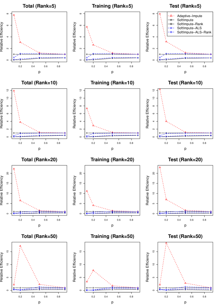
Figure 1: The relative efficiency plotted against the probability of observing each entry, $p$, when $\sigma=1$. Training errors are measured over the observed entries, test errors over the unobserved entries, and total errors over all entries.

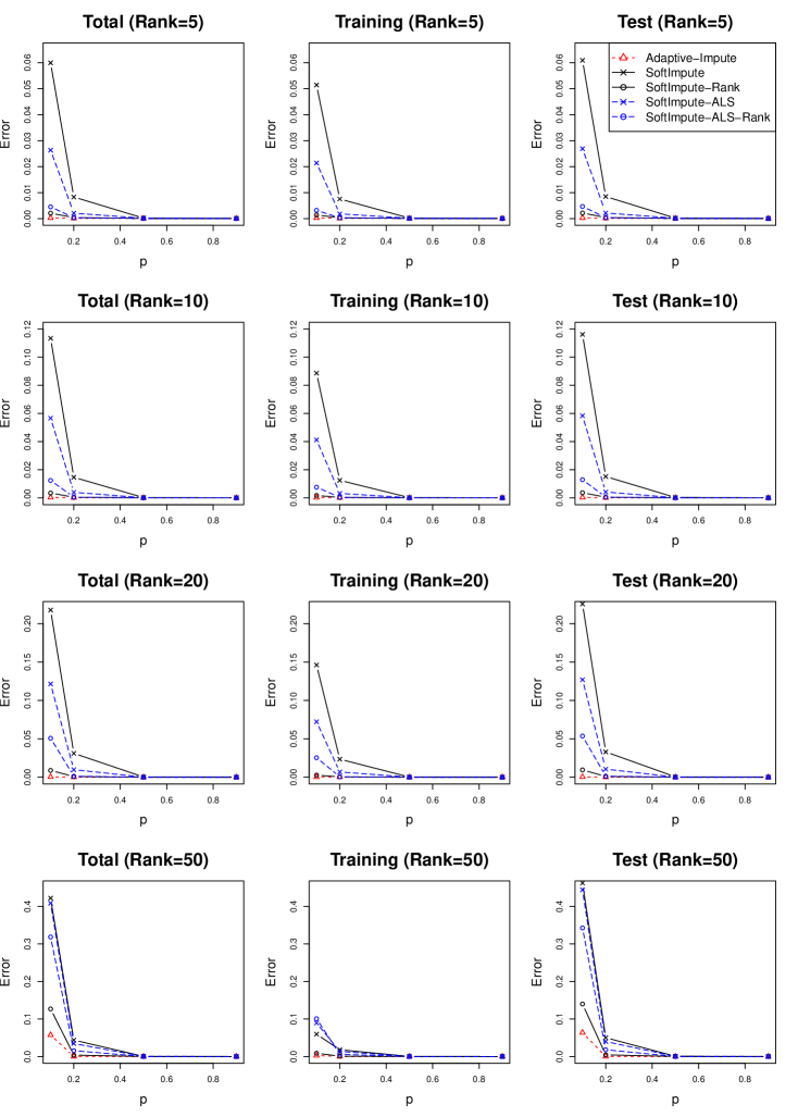
Figure 2: Change of the absolute errors when the probability of observing each entry, $p$ increases and $\sigma=1$.

Figure 1 shows the change of the relative efficiencies as the probability of observing each entry, $p$, increases with $\sigma=1$. Three columns of plots in Figure 1 correspond to three different types of errors and four rows of plots to four different values of the rank. In all cases, Adaptive-Impute outperforms the competitors and works especially better when $p$ is small. Among softImpute-type algorithms, the algorithms with rank constraint (i.e. softImpute-Rank and softImpute-ALS-Rank) perform better than the ones without (i.e. softImpute and softImpute-ALS). Figure 2 shows the change of the absolute errors that are used to compute relative efficiencies in Figure 1 as the probability of observing each entry, $p$, increases.

Figure 3 shows the change of the log relative efficiencies as the standard deviation (SD) of each entry of $\epsilon$, $\sigma$, increases with $p=0.1$. When the noise level is under 15, Adaptive-Impute outperforms the competitors, but when the noise level is over 15, softImpute-type algorithms start to outperform Adaptive-Impute. Hence, softImpute-type algorithms are more robust to large noises than Adaptive-Impute. It may be because when there exist large noises dominating the signals, the conditions for convergence presented in Section 4 are not satisfied. In real life applications, however, it is not common to observe such large noises that dominate the signals. Figure 4 shows the change of the absolute errors that are used to compute relative efficiencies in Figure 3.

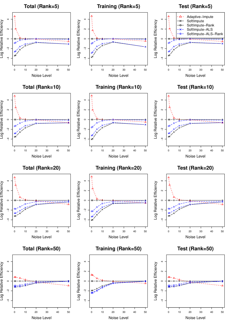
Figure 3: The log relative efficiency plotted against the SD of each entry of $\epsilon$ when $p=0.1$. Training errors are measured over the observed entries, test errors over the unobserved entries, and total errors over all entries.

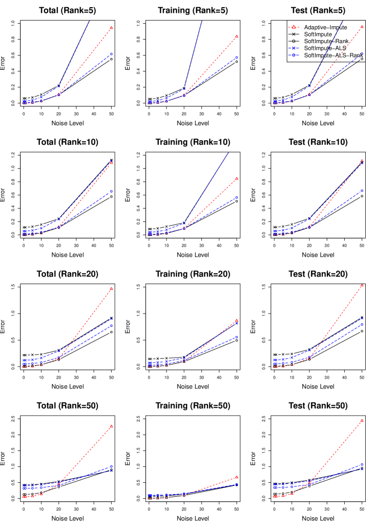
Figure 4: Change of the absolute errors when the SD of each entry of $\epsilon$ increases and $p=0.1$.

Figure 5 shows convergence of the iterates of Adaptive-Impute to the underlying low-rank matrix over iterations; that is, the change of log $\mbox{{Total}}(Z_{t}),\mbox{{Training}}(Z_{t})$, and $\mbox{{Test}}(Z_{t})$ errors as $t$ increases. Across all plots, $n=1700$, $d=1000$, $p=0.1$, and the errors were averaged over 100 replicates. In all cases, we observe that Adaptive-Impute converges well. Particularly, the smaller value of noise and/or rank is, the faster Adaptive-Impute converges.

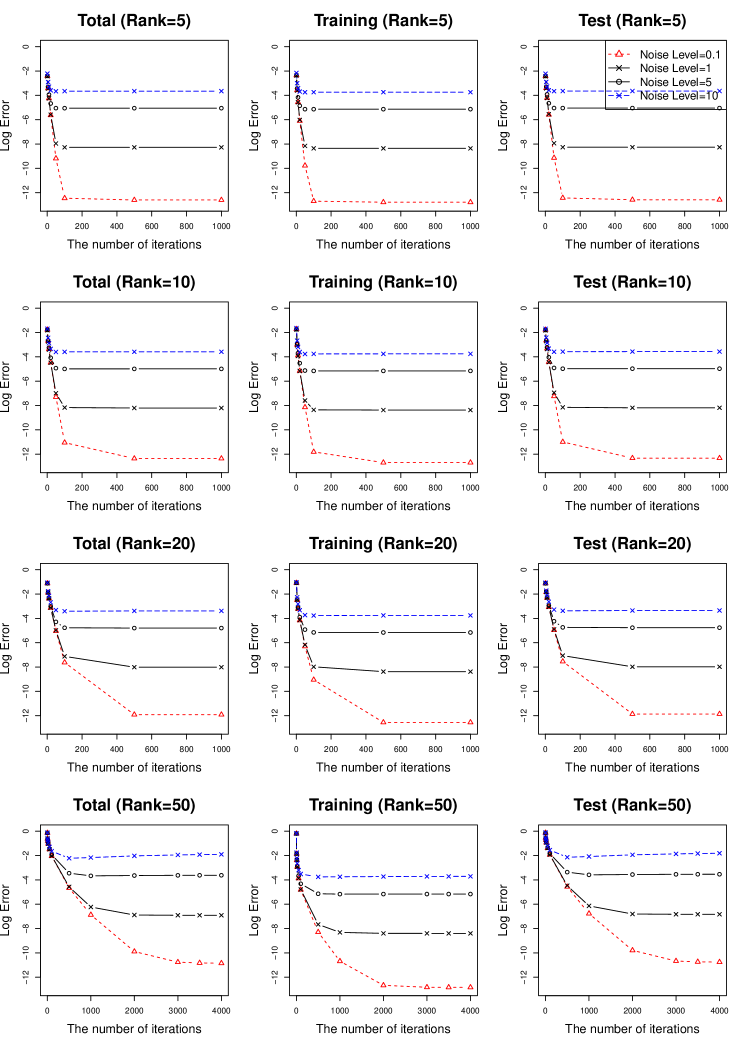
Figure 5: Convergence of the iterates of Adaptive-Impute to the underlying low-rank matrix. In all plots, $n=1700$, $d=1000$, $p=0.1$, and all points were averaged over 100 replicates.

5.2 A real data example

We applied Adaptive-Impute and the competing methods to a real data, MovieLens 100k (GroupLens (2015)). We used 5 training and 5 test data sets from 5-fold CV which are publicly available in GroupLens (2015). For the rank used in Adaptive-Impute and softImpute-type algorithms with rank constraint, we chose 3 based on a scree plot (Figure 6). Lemma 2 in Cho et al. (2016) provides justification of using the scree plot and the singular value gap to choose the rank.

Figure 6: Log of the top 50 singular values of the MovieLens 100k data matrix (GroupLens (2015)).

For the thresholding parameters for softImpute-type algorithms, we chose the optimal values which result in the smallest test errors. The test errors were measured by normalized mean absolute error (NMAE) (Herlocker et al. (2004)),

$$\frac{1}{(M_{max}-M_{min})|\Omega_{test}|}\sum_{(i,j)\in\Omega_{test}}|\hat{M}_{ij}-M_{ij}|,$$

where the set $\Omega_{test}$ contains indices of the entries in test data, $|\Omega_{test}|$ is the cardinality of $\Omega_{test}$, $M_{max}=\max\{\{M_{i,j}\}\setminus 0\}$ is the largest entry of $M$, and $M_{min}=\min\{\{M_{i,j}\}\setminus 0\}$ is the smallest entry of $M$.

Figure 7 summarizes the resulting NMAEs. Five points in the x-axis correspond to the 5-fold CV test data, the y-axis represents the values of NMAE, and the five different lines on the plane correspond to the 5 different algorithms in comparison. We observe that Adaptive-Impute outperforms all of the other algorithms. Specifically, the test errors of Adaptive-Impute reduce those of softImpute-type algorithms by 6%-16%. Among softImpute-type algorithms, the ones with rank constraint (i.e. softImpute-Rank and softImpute-ALS-Rank) performs better than the ones without (i.e. softImputeand softImpute-ALS). This is the same result to the simulation results.

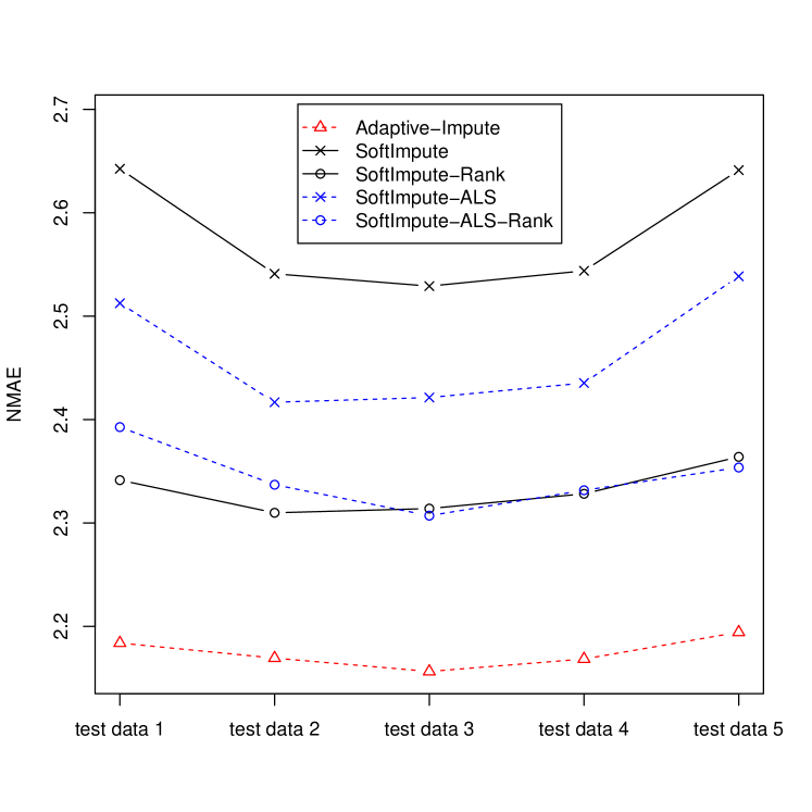
Figure 7: The NMAEs of Adaptive-Impute and its competitors measured in 5-fold CV test data from MovieLens 100k (GroupLens (2015)).

6 Discussion

Choosing the right thresholding parameter for matrix completion algorithms using thresholded SVD often poses empirical challenges. This paper proposed a novel thresholded SVD algorithm for matrix completion, Adaptive-Impute, which employs a theoretically-justified and data-dependent set of thresholding parameters. We established its theoretical guarantees on statistical performance and showed its strong performances in both simulated and real data. It provides understanding on the effects of thresholding and the right threshold level. Yet, there is a newly open problem. Although we proposed a reasonable remedy in the paper, the choice of the rank of the underlying low-rank matrix is of another great practical interest. To estimate the rank and completely automate the entire procedure of Adaptive-Impute would be a potential direction for future research.

7 Proofs

Denote by $C$ and $C_{1}$ generic constants whose values are free of $n$ and $p$ and may change from appearance to appearance. Also, denote by $\lVert v\rVert_{2}$ the $\ell_{2}$-norm for any vector $v\in\mathbb{R}^{d}$ and by $\lVert A\rVert_{2}$ the spectral norm, the largest singular value of $A$, for any matrix $A\in\mathbb{R}^{n\times d}$.

7.1 Proof of Theorem 3.1

Proof of Theorem 3.1.

We have

$$\widetilde{M}_{t} = \mathcal{P}_{\Omega}(M)+\mathcal{P}_{\Omega}^{\perp}(Z_{t})$$

$$= y\cdot(M_{0}+\epsilon)+(1_{n}1_{d}^{T}-y)\cdot Z_{t}$$

$$= M_{0}+y\cdot\epsilon+(1_{n}1_{d}^{T}-y)\cdot\eta_{t},$$

where $1_{n}$ and $1_{d}$ are vectors of length $n$ and $d$, respectively, filled with ones and $\eta_{t}=Z_{t}-M_{0}$, and, $A\cdot B=(A_{ij}B_{ij})_{1\leq i\leq n,1\leq j\leq d}$ for any $A$ and $B\in\mathbb{R}^{n\times d}$. Assume that

$$\frac{1}{\sqrt{nd}}\left\lVert\eta_{t}\right\rVert_{F}=o_{p}\left(\sqrt{\frac{h_{n}}{p\,d}}\right).$$ (12)

Then, simple algebraic manipulations show for large $n$

$$\frac{1}{\sqrt{nd}}\left\lVert\eta_{t+1}\right\rVert_{F} = \frac{1}{\sqrt{nd}}\left\lVert Z_{t+1}-M_{0}\right\rVert_{F}$$ (13)

$$= \frac{1}{\sqrt{nd}}\left\lVert\sum_{i=1}^{r}\sqrt{\bm{\mathbf{\lambda}}_{i}^{2}(\widetilde{M}_{t})-\widetilde{\bm{\mathbf{\alpha}}}_{t}}\,\mathbf{u}_{i}(\widetilde{M}_{t})\mathbf{v}_{i}(\widetilde{M}_{t})^{T}-\sum_{i=1}^{r}\lambda_{i}U_{i}V_{i}^{T}\right\rVert_{F}$$ (14)

$$\leq \frac{C}{\sqrt{nd}}\sum_{i=1}^{r}\Bigg{\{}\left|\sqrt{\bm{\mathbf{\lambda}}_{i}^{2}(\widetilde{M}_{t})-\widetilde{\bm{\mathbf{\alpha}}}_{t}}-\lambda_{i}\right|\left\lVert U_{i}V_{i}^{T}\right\rVert_{F}$$ (16)

$$\quad\quad\quad\quad+\lambda_{i}\left\lVert\left(\mathbf{u}_{i}(\widetilde{M}_{t})-U_{i}\mathcal{O}_{i}\right)V_{i}^{T}\right\rVert_{F}+\lambda_{i}\left\lVert U_{i}\left(\mathbf{v}_{i}(\widetilde{M}_{t})-V_{i}\mathcal{Q}_{i}\right)^{T}\right\rVert_{F}\Bigg{\}}$$

$$\leq C\sum_{i=1}^{r}\Bigg{\{}\frac{1}{\sqrt{nd}}\left|\sqrt{\bm{\mathbf{\lambda}}_{i}^{2}(\widetilde{M}_{t})-\widetilde{\bm{\mathbf{\alpha}}}_{t}}-\lambda_{i}\right|$$ (18)

$$\quad\quad\quad\quad+\frac{\lambda_{i}}{\sqrt{nd}}\left\lVert\mathbf{u}_{i}(\widetilde{M}_{t})-U_{i}\mathcal{O}_{i}\right\rVert_{F}+\frac{\lambda_{i}}{\sqrt{nd}}\left\lVert\mathbf{v}_{i}(\widetilde{M}_{t})-V_{i}\mathcal{Q}_{i}\right\rVert_{F}\Bigg{\}},$$

where $\mathcal{O}_{i}$ and $\mathcal{Q}_{i}$ are in $\{-1,1\}$ and minimize $\left\lVert\mathbf{u}_{i}(\widetilde{M}_{t})-U_{i}\mathcal{O}_{i}\right\rVert_{F}$ and $\left\lVert\mathbf{v}_{i}(\widetilde{M}_{t})-V_{i}\mathcal{Q}_{i}\right\rVert_{F}$, respectively.

To find the order of (13), first consider the term $\left\lVert\mathbf{v}_{i}(\widetilde{M}_{t})-V_{i}\mathcal{O}_{i}\right\rVert_{F}$. By Davis-Kahan Theorem (Theorem 3.1 in Li (1998b)) and Proposition 2.2 in Vu and Lei (2013),

$$\left\lVert\mathbf{v}_{i}(\widetilde{M}_{t})-V_{i}\mathcal{O}_{i}\right\rVert_{F}\leq\frac{\frac{1}{nd}\left\lVert\left(\widetilde{M}_{t}^{T}\widetilde{M}_{t}-\left[M_{0}^{T}M_{0}+np\sigma^{2}I\right]\right)V_{i}\right\rVert_{F}}{\left|\frac{1}{nd}\left(\lambda_{i}^{2}+np\sigma^{2}-\bm{\mathbf{\lambda}}_{i+1}^{2}(\widetilde{M}_{t})\right)\right|}.$$ (19)

Consider the numerator of (19). We have

$$\frac{1}{nd}\left\lVert\left(\widetilde{M}_{t}^{T}\widetilde{M}_{t}-\left[M_{0}^{T}M_{0}+np\sigma I\right]\right)V_{i}\right\rVert_{F}$$ (20)

$$\leq\frac{1}{nd}\bigg{\{}\left\lVert\left(y\cdot\epsilon\right)^{T}\left(y\cdot\epsilon\right)V_{i}-np\sigma^{2}V_{i}\right\rVert_{F}+\left\lVert\left[(1_{n}1_{d}^{T}-y)\cdot\eta_{t}\right]^{T}\left[(1_{n}1_{d}^{T}-y)\cdot\eta_{t}\right]V_{i}\right\rVert_{F}$$ (21)

$$\quad\quad\quad\quad+\left\lVert M_{0}^{T}\left(y\cdot\epsilon\right)V_{i}\right\rVert_{F}+\left\lVert\left(y\cdot\epsilon\right)^{T}M_{0}V_{i}\right\rVert_{F}$$ (22)

$$\quad\quad\quad\quad+\left\lVert M_{0}^{T}\left[(1_{n}1_{d}^{T}-y)\cdot\eta_{t}\right]V_{i}\right\rVert_{F}+\left\lVert\left[(1_{n}1_{d}^{T}-y)\cdot\eta_{t}\right]^{T}M_{0}V_{i}\right\rVert_{F}$$ (23)

$$\quad\quad\quad\quad+\left\lVert\left[(1_{n}1_{d}^{T}-y)\cdot\eta_{t}\right]^{T}\left(y\cdot\epsilon\right)V_{i}\right\rVert_{F}+\left\lVert\left(y\cdot\epsilon\right)^{T}\left[(1_{n}1_{d}^{T}-y)\cdot\eta_{t}\right]V_{i}\right\rVert_{F}\bigg{\}}$$ (24)

$$=\frac{1}{nd}\Big{\{}O_{p}\left(p\sqrt{nd}\right)+o_{p}\left(\frac{nh_{n}}{p}\right)+O_{p}\left(\sqrt{pdn^{2}}\right)+O_{p}\left(\sqrt{pd^{2}n}\right)$$ (25)

$$\quad\quad\quad\quad+o_{p}\left(\sqrt{\frac{h_{n}dn^{2}}{p}}\right)+o_{p}\left(\sqrt{\frac{h_{n}dn^{2}}{p}}\right)+o_{p}\left(\sqrt{h_{n}n^{2}}\right)+o_{p}\left(\sqrt{h_{n}dn^{2}}\right)\Big{\}}$$ (26)

$$=o_{p}\left(\sqrt{\frac{h_{n}}{pd}}\right),$$ (27)

where the first equality holds due to (1), Assumption 1(2), (12), and (28) and (33) below. We have

$$\mathbb{E}\left\lVert\left(y\cdot\epsilon\right)^{T}\left(y\cdot\epsilon\right)V_{i}-np\sigma^{2}V_{i}\right\rVert_{F}^{2}$$ (28)

$$=\mathbb{E}\left\{\sum_{h=1}^{d}\left[\sum_{k=1}^{n}\sum_{j=1}^{d}\left(y_{kh}y_{kj}\epsilon_{kh}\epsilon_{kj}V_{ij}-p\sigma^{2}V_{ih}\mathbbm{1}_{(j=h)}\right)\right]^{2}\right\}$$ (29)

$$=\sum_{h=1}^{d}\sum_{k=1}^{n}\sum_{j=1}^{d}\mathbb{E}\left(y_{kh}y_{kj}\epsilon_{kh}\epsilon_{kj}V_{ij}-p\sigma^{2}V_{ih}\mathbbm{1}_{(j=h)}\right)^{2}$$ (30)

$$=\sum_{k=1}^{n}\sum_{j\neq h}^{d}V_{ij}^{2}\,\mathbb{E}\left(y_{kh}^{2}y_{kj}^{2}\epsilon_{kh}^{2}\epsilon_{kj}^{2}\right)+\sum_{k=1}^{n}\sum_{j=h}^{d}V_{ij}^{2}\,\mathbb{E}\left(y_{kj}^{2}\epsilon_{kj}^{2}-p\sigma^{2}\right)^{2}$$ (31)

$$=O\left(p^{2}nd\right),$$ (32)

where $V_{ij}$ is the $j$-th element of $V_{i}$. Similarly, we have

$$\mathbb{E}\lVert\left(y\cdot\epsilon\right)V_{i}\rVert_{F}^{2}=O\left(pn\right),\mathbb{E}\lVert U_{i}^{T}\left(y\cdot\epsilon\right)\rVert_{F}^{2}=O\left(pd\right),\text{ and }\,\mathbb{E}\lVert y\cdot\epsilon\rVert_{F}^{2}=O\left(pnd\right).$$ (33)

Consider the denominator of (19). By Weyl’s theorem (Theorem 4.3 in Li (1998a)), we have

$$\max_{1\leq i\leq d}\frac{1}{nd}|\lambda_{i}^{2}+np\sigma^{2}-\bm{\mathbf{\lambda}}_{i}^{2}(\widetilde{M}_{t})|$$ (34)

$$\leq\frac{1}{nd}\left\lVert\widetilde{M}_{t}^{T}\widetilde{M}_{t}-\left[M_{0}^{T}M_{0}+np\sigma^{2}I\right]\right\rVert_{2}$$ (35)

$$\leq\frac{1}{nd}\bigg{\{}\left\lVert\left(y\cdot\epsilon\right)^{T}\left(y\cdot\epsilon\right)-np\sigma^{2}I\right\rVert_{2}+\left\lVert\left[(1_{n}1_{d}^{T}-y)\cdot\eta_{t}\right]^{T}\left[(1_{n}1_{d}^{T}-y)\cdot\eta_{t}\right]\right\rVert_{2}$$ (36)

$$\quad\quad\quad\quad+2\left\lVert M_{0}^{T}\left(y\cdot\epsilon\right)\right\rVert_{2}+2\left\lVert M_{0}^{T}\left[(1-y)\cdot\eta_{t}\right]\right\rVert_{2}+2\left\lVert\left(y\cdot\epsilon\right)^{T}\left[(1_{n}1_{d}^{T}-y)\cdot\eta_{t}\right]\right\rVert_{2}\bigg{\}}$$ (37)

$$=\frac{1}{nd}\bigg{\{}O_{p}\left(p\sqrt{nd^{2}}\right)+o_{p}\left(\frac{nh_{n}}{p}\right)+O_{p}\left(\sqrt{p\,dn^{2}}\right)+o_{p}\left(\sqrt{\frac{dn^{2}h_{n}}{p}}\right)+o_{p}\left(\sqrt{dn^{2}h_{n}}\right)\bigg{\}}$$ (38)

$$=o_{p}(1),$$ (39)

where the last two lines holds similarly to (20).

Thus, by (34) and (20),

$$\lVert\mathbf{v}_{i}(\widetilde{M}_{t})-V_{i}\mathcal{O}_{i}\rVert_{F}=o_{p}\left(\sqrt{\frac{h_{n}}{pd}}\right).$$ (40)

Secondly, similar to the proof of (40), we can show $\lVert\mathbf{u}_{i}(\widetilde{M}_{t})-U_{i}\mathcal{O}_{i}\rVert_{F}=o_{p}\left(\sqrt{h_{n}/pd}\right)$.

Lastly, consider the term $\frac{1}{\sqrt{nd}}\left|\sqrt{\bm{\mathbf{\lambda}}_{i}^{2}(\widetilde{M}_{t})-\widetilde{\bm{\mathbf{\alpha}}}_{t}}-\lambda_{i}\right|$. By Taylor’s expansion, there is $\lambda_{\ast}^{2}$ between $\bm{\mathbf{\lambda}}_{i}^{2}(\widetilde{M}_{t})-\widetilde{\bm{\mathbf{\alpha}}}_{t}$ and $\lambda_{i}^{2}$ such that

$$\frac{1}{\sqrt{nd}}\left|\sqrt{\bm{\mathbf{\lambda}}_{i}^{2}(\widetilde{M}_{t})-\widetilde{\bm{\mathbf{\alpha}}}_{t}}-\lambda_{i}\right|$$ (41)

$$=\frac{1}{\sqrt{nd}}\left|\frac{1}{2\lambda_{\ast}}\left(\bm{\mathbf{\lambda}}_{i}^{2}(\widetilde{M}_{t})-\widetilde{\bm{\mathbf{\alpha}}}_{t}-\lambda_{i}^{2}\right)\right|$$ (42)

$$\leq\frac{1}{2\lambda_{\ast}\sqrt{nd}}\left|\bm{\mathbf{\lambda}}_{i}^{2}(\widetilde{M}_{t})-(\lambda_{i}^{2}+np\sigma^{2})\right|+\frac{1}{2\lambda_{\ast}\sqrt{nd}}\left|\widetilde{\bm{\mathbf{\alpha}}}_{t}-np\sigma^{2}\right|.$$ (43)

We need to find the convergence rates of $\frac{1}{nd}\left|\bm{\mathbf{\lambda}}_{i}^{2}(\widetilde{M}_{t})-(\lambda_{i}^{2}+np\sigma^{2})\right|$ and $\frac{1}{nd}\left|\widetilde{\bm{\mathbf{\alpha}}}_{t}-np\sigma^{2}\right|$. Let $V_{c}=\left(V_{r+1},\ldots,V_{d}\right)\in\mathbb{R}^{d\times(d-r)}$ be a matrix such that $V_{c}^{T}V_{c}=I_{d-r}$ and $V^{T}V_{c}=0_{r\times(d-r)}$ and let $\widetilde{V}_{t}=\left(\mathbf{v}_{1}(\widetilde{M}_{t}),\ldots,\mathbf{v}_{d}(\widetilde{M}_{t})\right)\in\mathbb{R}^{d\times r}$ and $\widetilde{V}_{tc}=\left(\mathbf{v}_{r+1}(\widetilde{M}_{t}),\ldots,\mathbf{v}_{d}(\widetilde{M}_{t})\right)\in\mathbb{R}^{d\times(d-r)}$ so that $\widetilde{V}_{t}^{T}\widetilde{V}_{tc}=0_{r\times(d-r)}$. Also, let $\mathcal{O}=\text{diag}(\mathcal{O}_{1},\ldots,\mathcal{O}_{r})$ and $\mathcal{O}_{c}=\text{diag}(\mathcal{O}_{r+1},\ldots,\mathcal{O}_{d})$, where

$$\mathcal{O}_{i}:=\operatornamewithlimits{arg\,min}_{o\in\{-1,1\}}\left\lVert V_{i}\,o-\mathbf{v}_{i}(\widetilde{M}_{t})\right\rVert_{2}^{2}\quad\text{for }\;i=1,\ldots,d.$$

Then, we have

$$\frac{1}{nd}\left|\bm{\mathbf{\lambda}}_{i}^{2}(\widetilde{M}_{t})-(\lambda_{i}^{2}+np\sigma^{2})\right|$$ (44)

$$=\frac{1}{nd}\bigg{|}\mathbf{v}_{i}(\widetilde{M}_{t})^{T}\widetilde{M}_{t}^{T}\widetilde{M}_{t}\mathbf{v}_{i}(\widetilde{M}_{t})-V_{i}^{T}\left({M_{0}}^{T}{M_{0}}+np\sigma^{2}I\right)V_{i}\bigg{|}$$ (45)

$$\leq\frac{1}{nd}\bigg{|}V_{i}^{T}\left[\widetilde{M}_{t}^{T}\widetilde{M}_{t}-\left({M_{0}}^{T}{M_{0}}+np\sigma^{2}I\right)\right]V_{i}\bigg{|}+\frac{1}{nd}\bigg{|}\mathbf{v}_{i}(\widetilde{M}_{t})^{T}\widetilde{M}_{t}^{T}\widetilde{M}_{t}\mathbf{v}_{i}(\widetilde{M}_{t})-V_{i}^{T}\widetilde{M}_{t}^{T}\widetilde{M}_{t}V_{i}\bigg{|}$$ (46)

$$\leq o_{p}\left(\sqrt{\frac{h_{n}}{pd}}\right)+\frac{1}{nd}\bigg{|}\mathbf{v}_{i}(\widetilde{M}_{t})^{T}\widetilde{M}_{t}^{T}\widetilde{M}_{t}\mathbf{v}_{i}(\widetilde{M}_{t})-V_{i}^{T}\widetilde{M}_{t}^{T}\widetilde{M}_{t}V_{i}\bigg{|}$$ (47)

$$=o_{p}\left(\sqrt{\frac{h_{n}}{pd}}\right),$$ (48)

where the second inequality can be derived by the similar way to the proof of (20), and the last equality is due to (49) below. Simple algebraic manipulations show

$$\frac{1}{nd}\bigg{|}\mathbf{v}_{i}(\widetilde{M}_{t})^{T}\widetilde{M}_{t}^{T}\widetilde{M}_{t}\mathbf{v}_{i}(\widetilde{M}_{t})-V_{i}^{T}\widetilde{M}_{t}^{T}\widetilde{M}_{t}V_{i}\bigg{|}$$ (49)

$$=\frac{1}{nd}\bigg{|}\left[V_{i}\mathcal{O}_{i}-\mathbf{v}_{i}(\widetilde{M}_{t})\right]^{T}\widetilde{M}_{t}^{T}\widetilde{M}_{t}\left[V_{i}\mathcal{O}_{i}-\mathbf{v}_{i}(\widetilde{M}_{t})\right]+2\bm{\mathbf{\lambda}}_{i}^{2}(\widetilde{M}_{t})\left[V_{i}\mathcal{O}_{i}-\mathbf{v}_{i}(\widetilde{M}_{t})\right]^{T}\mathbf{v}_{i}(\widetilde{M}_{t})\bigg{|}$$ (50)

$$\leq\frac{2\bm{\mathbf{\lambda}}_{1}^{2}(\widetilde{M}_{t})}{nd}\left\lVert V_{i}\mathcal{O}_{i}-\mathbf{v}_{i}(\widetilde{M}_{t})\right\rVert_{2}^{2}$$ (51)

$$=o_{p}\left(\frac{h_{n}}{pd}\right),$$ (52)

where the last equality is due to (34) and (40). Also,

$$\frac{1}{nd}\left|\widetilde{\bm{\mathbf{\alpha}}}_{t}-np\sigma^{2}\right|$$ (53)

$$=\frac{1}{nd}\bigg{|}\frac{1}{d-r}\sum_{j=r+1}^{d}\mathbf{v}_{j}(\widetilde{M}_{t})^{T}\widetilde{M}_{t}^{T}\widetilde{M}_{t}\mathbf{v}_{j}(\widetilde{M}_{t})-np\sigma^{2}\bigg{|}$$ (54)

$$\leq\frac{1}{nd}\bigg{|}\frac{1}{d-r}\sum_{j=r+1}^{d}V_{j}^{T}\left[\widetilde{M}_{t}^{T}\widetilde{M}_{t}-\left(M_{0}^{T}M_{0}+np\sigma^{2}I\right)\right]V_{j}\bigg{|}$$ (55)

$$\quad\quad\quad\quad+\frac{1}{nd}\bigg{|}\frac{1}{d-r}\sum_{j=r+1}^{d}\left[\mathbf{v}_{j}(\widetilde{M}_{t})^{T}\widetilde{M}_{t}^{T}\widetilde{M}_{t}\mathbf{v}_{j}(\widetilde{M}_{t})-V_{j}^{T}\widetilde{M}_{t}^{T}\widetilde{M}_{t}V_{j}\right]\bigg{|}$$ (56)

$$=o_{p}\left(\sqrt{\frac{h_{n}}{pd}}\right)+\frac{1}{nd}\bigg{|}\frac{1}{d-r}\sum_{j=r+1}^{d}\left[\mathbf{v}_{j}(\widetilde{M}_{t})^{T}\widetilde{M}_{t}^{T}\widetilde{M}_{t}\mathbf{v}_{j}(\widetilde{M}_{t})-V_{j}^{T}\widetilde{M}_{t}^{T}\widetilde{M}_{t}V_{j}\right]\bigg{|}$$ (57)

$$=o_{p}\left(\sqrt{\frac{h_{n}}{pd}}\right),$$ (58)

where the second equality can be derived by the similar way to the proof of (20), and the last equality is due to (59) below. Similar to the proof of (49), we have

$$\frac{1}{nd(d-r)}\sum_{j=r+1}^{d}\bigg{|}\mathbf{v}_{j}(\widetilde{M}_{t})^{T}\widetilde{M}_{t}^{T}\widetilde{M}_{t}\mathbf{v}_{j}(\widetilde{M}_{t})-V_{j}^{T}\widetilde{M}_{t}^{T}\widetilde{M}_{t}V_{j}\bigg{|}$$ (59)

$$\leq\frac{1}{nd(d-r)}\sum_{j=r+1}^{d}2\bm{\mathbf{\lambda}}_{1}^{2}(\widetilde{M}_{t})\left\lVert V_{j}\mathcal{O}_{j}-\mathbf{v}_{j}(\widetilde{M}_{t})\right\rVert_{2}^{2}$$ (60)

$$\leq\frac{2\bm{\mathbf{\lambda}}_{1}^{2}(\widetilde{M}_{t})}{nd(d-r)}\left\lVert V_{c}\mathcal{O}_{c}-\widetilde{V}_{tc}\right\rVert_{F}^{2}$$ (61)

$$\leq\frac{4\bm{\mathbf{\lambda}}_{1}^{2}(\widetilde{M}_{t})}{nd(d-r)}\left\lVert V_{c}V_{c}^{T}-\widetilde{V}_{tc}\widetilde{V}_{tc}^{T}\right\rVert_{F}^{2}$$ (62)

$$=\frac{4\bm{\mathbf{\lambda}}_{1}^{2}(\widetilde{M}_{t})}{nd(d-r)}\left\lVert VV^{T}-\widetilde{V}_{t}\widetilde{V}_{t}^{T}\right\rVert_{F}^{2}$$ (63)

$$\leq\frac{4\bm{\mathbf{\lambda}}_{1}^{2}(\widetilde{M}_{t})}{nd(d-r)}\left\lVert V\mathcal{O}-\widetilde{V}_{t}\right\rVert_{F}^{2}$$ (64)

$$=\frac{4\bm{\mathbf{\lambda}}_{1}^{2}(\widetilde{M}_{t})}{nd(d-r)}\sum_{i=1}^{r}\left\lVert V_{i}\mathcal{O}_{i}-\mathbf{v}_{i}(\widetilde{M}_{t})\right\rVert_{2}^{2}$$ (65)

$$=o_{p}\left(\frac{h_{n}}{pd^{2}}\right),$$ (66)

where the fourth and sixth lines are due to Proposition 2.2 in Vu and Lei (2013), and the last line holds from (40).

The three results above (41), (44), and (53) give $\frac{1}{\sqrt{nd}}\left|\sqrt{\bm{\mathbf{\lambda}}_{i}^{2}(\widetilde{M}_{t})-\widetilde{\bm{\mathbf{\alpha}}}_{t}}-\lambda_{i}\right|=o_{p}\left(\sqrt{\frac{h_{n}}{pd}}\right)$.

Therefore, combining the results above, we have that $\frac{1}{\sqrt{nd}}\left\lVert\eta_{t+1}\right\rVert_{F}$ in (13) is $o_{p}\left(\sqrt{\frac{h_{n}}{pd}}\right)$. Since $\frac{1}{\sqrt{nd}}\left\lVert\eta_{1}\right\rVert_{F}=o_{p}\left(\sqrt{\frac{h_{n}}{pd}}\right)$ by Proposition 3.1, we have $\frac{1}{\sqrt{nd}}\left\lVert\eta_{t}\right\rVert_{F}=o_{p}\left(\sqrt{\frac{h_{n}}{pd}}\right)$ for any fixed $t$ by mathematical induction. ∎

7.2 Proof of Theorem 3.2

Proof of Theorem 3.2.

We have

$$\min_{Z}\;\frac{1}{2nd}\left\lVert X-Z\right\rVert_{F}^{2}+\sum_{i=1}^{d}\frac{\tau_{i}}{\sqrt{nd}}\frac{\bm{\mathbf{\lambda}}_{i}(Z)}{\sqrt{nd}}$$ (67)

$$=\min_{Z}\;\frac{1}{2nd}\Bigg{\{}\left\lVert X\right\rVert_{F}^{2}-2\sum_{i=1}^{d}\tilde{\lambda}_{i}\cdot\tilde{u}_{i}^{T}X\tilde{v}_{i}+\sum_{i=1}^{d}\tilde{\lambda}_{i}^{2}\Bigg{\}}+\frac{1}{nd}\sum_{i=1}^{d}\tau_{i}\tilde{\lambda}_{i},$$ (68)

where $\tilde{\lambda}_{i}=\bm{\mathbf{\lambda}}_{i}(Z)$, $\tilde{u}_{i}=\mathbf{u}_{i}(Z)$, and $\tilde{v}_{i}=\mathbf{v}_{i}(Z)$. Minimizing (67) is equivalent to minimizing

$$-2\sum_{i=1}^{d}\tilde{\lambda}_{i}\cdot\tilde{u}_{i}^{T}X\tilde{v}_{i}+\sum_{i=1}^{d}\tilde{\lambda}_{i}^{2}+\sum_{i=1}^{d}2\tau_{i}\tilde{\lambda}_{i},$$

with respect to $\tilde{\lambda}_{i},\tilde{u}_{i},$ and $\tilde{v}_{i},\;i=1,\ldots,d$, under the conditions that $(\tilde{u}_{1},\ldots,\tilde{u}_{d})^{T}(\tilde{u}_{1},\ldots,\tilde{u}_{d})=I_{d}$, $(\tilde{v}_{1},\ldots,\tilde{v}_{d})^{T}(\tilde{v}_{1},\ldots,\tilde{v}_{d})=I_{d}$, and $\tilde{\lambda}_{1}\geq\tilde{\lambda}_{2}\geq\ldots\geq\tilde{\lambda}_{d}\geq 0$. Thus, we have

$$\min_{\tilde{\lambda}_{i}\geq 0,\tilde{u}_{i},\tilde{v}_{i},\;i=1,\ldots,d}\;-2\sum_{i=1}^{d}\tilde{\lambda}_{i}\cdot\tilde{u}_{i}^{T}X\tilde{v}_{i}+\sum_{i=1}^{d}\tilde{\lambda}_{i}^{2}+\sum_{i=1}^{d}2\tau_{i}\tilde{\lambda}_{i}$$ (69)

$$=\min_{\tilde{\lambda}_{i}\geq 0,\;i=1,\ldots,d}\;-2\sum_{i=1}^{d}\tilde{\lambda}_{i}\cdot\bm{\mathbf{\lambda}}_{i}(X)+\sum_{i=1}^{d}\tilde{\lambda}_{i}^{2}+\sum_{i=1}^{d}2\tau_{i}\tilde{\lambda}_{i}$$ (70)

$$=\min_{\tilde{\lambda}_{i}\geq 0,\;i=1,\ldots,d}\;\sum_{i=1}^{d}\left\{\tilde{\lambda}_{i}^{2}-2\tilde{\lambda}_{i}\left[\bm{\mathbf{\lambda}}_{i}(X)-\tau_{i}\right]\right\},$$ (71)

where the first equality is due to the facts that $\tilde{\lambda}_{1}\geq\ldots\geq\tilde{\lambda}_{d}\geq 0$, and for every $i$, the problem

$$\max_{\left\lVert u_{i}\right\rVert_{2}^{2}\leq 1,\left\lVert v_{i}\right\rVert_{2}^{2}\leq 1}u_{i}^{T}Xv_{i}\quad\text{such that}\quad u_{i}\perp\{\tilde{u}_{1}^{\ast},\ldots,\tilde{u}_{i-1}^{\ast}\},v_{i}\perp\{\tilde{v}_{1}^{\ast},\ldots,\tilde{v}_{i-1}^{\ast}\}$$

is solved by $\tilde{u}_{i}^{\ast},\tilde{v}_{i}^{\ast}$, the left and right singular vectors of $X$ corresponding to the $i$-th largest singular value of $X$. Note that $\tilde{u}_{i}=\tilde{u}_{i}^{\ast}$. Since (69) is a quadratic function of $\tilde{\lambda}_{i}$, the solution to the problem (69) is then $\tilde{\lambda}_{i}=\left(\bm{\mathbf{\lambda}}_{i}(X)-\tau_{i}\right)_{+}$. ∎

7.3 Proof of Theorem 4.1

To ease the notation, we drop the superscript ‘g’ in $Z_{t}^{g}$, $\widetilde{M}_{t}^{g}$, and $D_{t}^{g}$ in this section.

Lemma 7.1.

Let $Z_{t+1}:=\operatornamewithlimits{arg\,min}_{Z\in\mathbb{R}^{n\times d}}Q_{\tau}(Z|Z_{t})$ in (9). Then, under Assumption 3, we have

$$\left\lVert Z_{t+1}-Z_{t}\right\rVert_{F}^{2}\to 0\quad\text{as }t\to\infty.$$

Proof of Lemma 7.1.

By the construction of $D_{t}$,

$$(\widetilde{M}_{t-1}-\widetilde{M}_{t})-(Z_{t}-Z_{t+1})-(D_{t-1}-D_{t})=0.$$

Thus, we have

$$\langle\widetilde{M}_{t-1}-\widetilde{M}_{t},Z_{t}-Z_{t+1}\rangle-\langle Z_{t}-Z_{t+1},Z_{t}-Z_{t+1}\rangle-\langle D_{t-1}-D_{t},Z_{t}-Z_{t+1}\rangle=0$$ (72)

and

$$\langle\widetilde{M}_{t-1}-\widetilde{M}_{t},\widetilde{M}_{t-1}-\widetilde{M}_{t}\rangle-\langle Z_{t}-Z_{t+1},\widetilde{M}_{t-1}-\widetilde{M}_{t}\rangle-\langle D_{t-1}-D_{t},\widetilde{M}_{t-1}-\widetilde{M}_{t}\rangle=0.$$ (73)

Add (73) and (72), and

$$0=\lVert\widetilde{M}_{t-1}-\widetilde{M}_{t}\rVert_{F}^{2}-\lVert Z_{t}-Z_{t+1}\rVert_{F}^{2}-\langle D_{t-1}-D_{t},Z_{t}+\widetilde{M}_{t-1}-(Z_{t+1}+\widetilde{M}_{t})\rangle$$ (74)

$$=\lVert\widetilde{M}_{t-1}-\widetilde{M}_{t}\rVert_{F}^{2}-\lVert Z_{t}-Z_{t+1}\rVert_{F}^{2}-\left\lVert D_{t-1}-D_{t}\right\rVert_{F}^{2}-2\langle D_{t-1}-D_{t},Z_{t}-Z_{t+1}\rangle.$$ (75)

Under Assumption 3, (74) gives

$$\left\lVert Z_{t}-Z_{t+1}\right\rVert_{F}^{2}\leq\left\lVert\widetilde{M}_{t-1}-\widetilde{M}_{t}\right\rVert_{F}^{2},$$

and thus

$$\left\lVert Z_{t+1}-Z_{t}\right\rVert_{F}^{2} \leq \left\lVert\widetilde{M}_{t-1}-\widetilde{M}_{t}\right\rVert_{F}^{2}$$ (76)

$$\leq \left\lVert\mathcal{P}_{\Omega}^{\perp}\left(Z_{t-1}-Z_{t}\right)\right\rVert_{F}^{2}$$ (77)

$$\leq \left\lVert Z_{t}-Z_{t-1}\right\rVert_{F}^{2}$$ (78)

for all $t\geq 1$. This proves that the sequence $\{\left\lVert Z_{t+1}-Z_{t}\right\rVert_{F}^{2}\}$ converges (since it is decreasing and bounded below).

The convergence of $\{\left\lVert Z_{t+1}-Z_{t}\right\rVert_{F}^{2}\}$ gives

$$\left\lVert Z_{t+1}-Z_{t}\right\rVert_{F}^{2}-\left\lVert Z_{t}-Z_{t-1}\right\rVert_{F}^{2}\to 0\text{ as }t\to\infty.$$

Then, by (76),

$$0 \geq \left\lVert\mathcal{P}_{\Omega}^{\perp}\left(Z_{t}-Z_{t-1}\right)\right\rVert_{F}^{2}-\left\lVert Z_{t}-Z_{t-1}\right\rVert_{F}^{2}$$

$$\geq \left\lVert Z_{t+1}-Z_{t}\right\rVert_{F}^{2}-\left\lVert Z_{t}-Z_{t-1}\right\rVert_{F}^{2}$$

$$\to 0\quad\text{as }t\to\infty,$$

which implies

$$\left\lVert\mathcal{P}_{\Omega}^{\perp}\left(Z_{t}-Z_{t-1}\right)\right\rVert_{F}^{2}-\left\lVert Z_{t}-Z_{t-1}\right\rVert_{F}^{2}\to 0\Rightarrow\left\lVert\mathcal{P}_{\Omega}\left(Z_{t}-Z_{t-1}\right)\right\rVert_{F}^{2}\to 0.$$ (79)

Furthermore, similarly to the proof of Lemma 2 in Mazumder et al. (2010), we can show

$$f_{\tau}(Z_{t})\geq Q_{\tau}(Z_{t+1}|Z_{t})\geq Q_{\tau}(Z_{t+1}|Z_{t+1})=f_{\tau}(Z_{t+1})\geq 0$$ (80)

for every fixed $\tau_{1},\ldots,\tau_{d}>0$ and $t\geq 1$. Thus, we have

$$Q_{\tau}(Z_{t+1}|Z_{t})-Q_{\tau}(Z_{t+1}|Z_{t+1})\to 0\quad\text{as }t\to\infty,$$

which implies

$$\left\lVert\mathcal{P}_{\Omega}^{\perp}\left(Z_{t}-Z_{t+1}\right)\right\rVert_{F}^{2}\to 0\quad\text{as }t\to\infty.$$

The above along with (79) gives

$$\left\lVert Z_{t+1}-Z_{t}\right\rVert_{F}^{2}\to 0\quad\text{as }t\to\infty.$$

∎

Proof of Theorem 4.1.

By the construction of $D_{t}$, we have

$$0=\left(\widetilde{M}_{t}-Z_{t+1}\right)-D_{t}\quad\text{for all }t\geq 1.$$

Since $Z_{\infty}$ is a limit point of the sequence $Z_{t}$, there exists a subsequence $\{n_{t}\}\subset\{1,2,\ldots\}$ such that $Z_{n_{t}}\to Z_{\infty}$ as $t\to\infty$. By Lemma 7.1, this subsequence $Z_{n_{t}}$ satisfies

$$Z_{n_{t}}-Z_{n_{t}+1}\to 0$$

which implies

$$\mathcal{P}_{\Omega}^{\perp}(Z_{n_{t}})-Z_{n_{t}+1}\to\mathcal{P}_{\Omega}^{\perp}(Z_{\infty})-Z_{\infty}=-\mathcal{P}_{\Omega}(Z_{\infty}).$$

Hence,

$$D_{n_{t}}=\left(\mathcal{P}_{\Omega}(M)+\mathcal{P}_{\Omega}^{\perp}(Z_{n_{t}})\right)-Z_{n_{t}+1}\to\mathcal{P}_{\Omega}(M)-\mathcal{P}_{\Omega}(Z_{\infty})=D_{\infty}.$$ (81)

Due to (11) and (81), we have

$$f_{\tau}(Z^{s}) \geq f_{\tau}(Z_{\infty})-\frac{1}{nd}\langle Z^{s}-Z_{\infty},\mathcal{P}_{\Omega}(M)-\mathcal{P}_{\Omega}(Z_{\infty})-D_{\infty}\rangle$$

$$= f_{\tau}(Z_{\infty}).$$

Since $f_{\tau}(Z^{s})\leq f_{\tau}(Z_{\infty})$ by definition of $Z^{s}$, we have $f_{\tau}(Z^{s})=f_{\tau}(Z_{\infty})$. Lastly, by (80), we have $\lim_{t\rightarrow\infty}f_{\tau}(Z_{t})=f(Z^{s})$. ∎

7.4 Proofs of Lemmas 4.1-4.2

Proof of Lemma 4.1.

For $i=1,\ldots,r$, we have

$$\left|\frac{\tau_{t,i}}{\sqrt{nd}}-\frac{\tau_{t+1,i}}{\sqrt{nd}}\right|$$

$$=\frac{1}{\sqrt{nd}}\left|\bm{\mathbf{\lambda}}_{i}(\widetilde{M}_{t})-\sqrt{\bm{\mathbf{\lambda}}_{i}^{2}(\widetilde{M}_{t})-\widetilde{\bm{\mathbf{\alpha}}}_{t}}-\lambda_{i}(\widetilde{M}_{t+1})+\sqrt{\bm{\mathbf{\lambda}}_{i}^{2}(\widetilde{M}_{t+1})-\widetilde{\bm{\mathbf{\alpha}}}_{t+1}}\right|$$

$$\leq\frac{1}{\sqrt{nd}}\left|\bm{\mathbf{\lambda}}_{i}(\widetilde{M}_{t})-\left(\sqrt{\lambda_{i}^{2}-np\sigma^{2}}\right)\right|+\frac{1}{\sqrt{nd}}\left|\sqrt{\bm{\mathbf{\lambda}}_{i}^{2}(\widetilde{M}_{t})-\widetilde{\bm{\mathbf{\alpha}}}_{t}}-\lambda_{i}^{2}\right|$$

$$\quad+\frac{1}{\sqrt{nd}}\left|\bm{\mathbf{\lambda}}_{i}(\widetilde{M}_{t+1})-\left(\sqrt{\lambda_{i}^{2}-np\sigma^{2}}\right)\right|+\frac{1}{\sqrt{nd}}\left|\sqrt{\bm{\mathbf{\lambda}}_{i}^{2}(\widetilde{M}_{t+1})-\widetilde{\bm{\mathbf{\alpha}}}_{t+1}}-\lambda_{i}^{2}\right|$$

$$=(I)+(II)+(III)+(IV).$$

Then, by (44) and (53), we have

$$(I) = \frac{1}{\sqrt{nd}}\left|\bm{\mathbf{\lambda}}_{i}(\widetilde{M}_{t})-\left(\sqrt{\lambda_{i}^{2}-np\sigma^{2}}\right)\right|$$

$$= \frac{1}{2\lambda_{\ast}\sqrt{nd}}\left|\bm{\mathbf{\lambda}}_{i}^{2}(\widetilde{M}_{t})-\left(\lambda_{i}^{2}-np\sigma^{2}\right)\right|$$

$$\leq \frac{1}{2\lambda_{\ast}\sqrt{nd}}\left|\bm{\mathbf{\lambda}}_{i}^{2}(\widetilde{M}_{t})-\widetilde{\bm{\mathbf{\alpha}}}_{t}-\lambda_{i}^{2}\right|+\frac{1}{2\lambda_{\ast}\sqrt{nd}}\left|\widetilde{\bm{\mathbf{\alpha}}}_{t}-np\sigma^{2}\right|$$

$$= o_{p}\left(\sqrt{\frac{h_{n}}{pd}}\right),$$

where the second equality holds for some $\lambda_{\ast}$ between $\bm{\mathbf{\lambda}}_{i}(\widetilde{M}_{t})$ and $\sqrt{\lambda_{i}^{2}-np\sigma^{2}}$ by Taylor’s expansion. We can similarly show that $(III)=o_{p}\left(\sqrt{h_{n}/pd}\right)$. Both of $(II)$ and $(IV)$ are also $o_{p}\left(\sqrt{h_{n}/pd}\right)$ by (41) and (44). ∎

Proof of Lemma 4.2.

From Theorem 3.1 and the construction of $D_{t}$ in Assumption 3, we have

$$\left|\frac{1}{nd}\langle D_{t}-D_{t+1},Z_{t+1}-Z_{t+2}\rangle\right|$$

$$\leq\frac{1}{nd}\left\lVert D_{t}-D_{t+1}\right\rVert_{F}\left\lVert Z_{t+1}-Z_{t+2}\right\rVert_{F}$$

$$\leq\frac{1}{nd}\left\lVert\widetilde{M}_{t}-Z_{t+1}-\left(\widetilde{M}_{t+1}-Z_{t+2}\right)\right\rVert_{F}\left\lVert Z_{t+1}-Z_{t+2}\right\rVert_{F}$$

$$\leq\frac{1}{nd}\Big{\{}\left\lVert\widetilde{M}_{t}-\widetilde{M}_{t+1}\right\rVert_{F}+\left\lVert Z_{t+1}-Z_{t+2}\right\rVert_{F}\Big{\}}\left\lVert Z_{t+1}-Z_{t+2}\right\rVert_{F}$$

$$=\frac{1}{nd}\Big{\{}\left\lVert\mathcal{P}_{\Omega}^{\perp}\left(Z_{t}-Z_{t+1}\right)\right\rVert_{F}+\left\lVert Z_{t+1}-Z_{t+2}\right\rVert_{F}\Big{\}}\left\lVert Z_{t+1}-Z_{t+2}\right\rVert_{F}$$

$$\leq\frac{1}{nd}\Big{\{}\left\lVert Z_{t}-Z_{t+1}\right\rVert_{F}+\left\lVert Z_{t+1}-Z_{t+2}\right\rVert_{F}\Big{\}}\left\lVert Z_{t+1}-Z_{t+2}\right\rVert_{F}$$

$$\leq\frac{1}{nd}\Big{\{}\left\lVert Z_{t}-M_{0}\right\rVert_{F}+2\left\lVert Z_{t+1}-M_{0}\right\rVert_{F}+\left\lVert Z_{t+2}-M_{0}\right\rVert_{F}\Big{\}}$$

$$\quad\times\Big{\{}\left\lVert Z_{t+1}-M_{0}\right\rVert_{F}+\left\lVert Z_{t+2}-M_{0}\right\rVert_{F}\Big{\}}$$

$$=o_{p}\left(\frac{h_{n}}{pd}\right).$$

∎

References

- Achlioptas and McSherry (2001) Achlioptas, D. and F. McSherry (2001). Fast computation of low rank matrix approximations. In Proceedings of the thirty-third annual ACM symposium on Theory of computing, pp. 611–618. ACM.
- Azar et al. (2001) Azar, Y., A. Fiat, A. Karlin, F. McSherry, and J. Saia (2001). Spectral analysis of data. In Proceedings of the thirty-third annual ACM symposium on Theory of computing, pp. 619–626. ACM.
- Bennett and Lanning (2007) Bennett, J. and S. Lanning (2007). The netflix prize. In Proceedings of KDD cup and workshop, Volume 2007, pp. 35.
- Cai et al. (2010) Cai, J.-F., E. J. Candès, and Z. Shen (2010). A singular value thresholding algorithm for matrix completion. SIAM Journal on Optimization 20(4), 1956–1982.
- Cai and Liu (2011) Cai, T. and W. Liu (2011). Adaptive thresholding for sparse covariance matrix estimation. Journal of the American Statistical Association 106(494), 672–684.
- Cai and Zhou (2013) Cai, T. T. and W.-X. Zhou (2013). Matrix completion via max-norm constrained optimization. arXiv preprint arXiv:1303.0341.
- Candès and Plan (2010) Candès, E. J. and Y. Plan (2010). Matrix completion with noise. Proceedings of the IEEE 98(6), 925–936.
- Candès and Recht (2009) Candès, E. J. and B. Recht (2009). Exact matrix completion via convex optimization. Foundations of Computational mathematics 9(6), 717–772.
- Candès et al. (2006) Candès, E. J., J. Romberg, and T. Tao (2006). Robust uncertainty principles: Exact signal reconstruction from highly incomplete frequency information. Information Theory, IEEE Transactions on 52(2), 489–509.
- Candès and Tao (2010) Candès, E. J. and T. Tao (2010). The power of convex relaxation: Near-optimal matrix completion. Information Theory, IEEE Transactions on 56(5), 2053–2080.
- Chatterjee (2014) Chatterjee, S. (2014). Matrix estimation by universal singular value thresholding. The Annals of Statistics 43(1), 177–214.
- Cho et al. (2016) Cho, J., D. Kim, and K. Rohe (2016). Asymptotic theory for estimating the singular vectors and values of a partially-observed low rank matrix with noise.
- Davenport et al. (2014) Davenport, M. A., Y. Plan, E. van den Berg, and M. Wootters (2014). 1-bit matrix completion. Information and Inference 3(3), 189–223.
- Donoho (2006) Donoho, D. L. (2006). Compressed sensing. Information Theory, IEEE Transactions on 52(4), 1289–1306.
- Fan et al. (2013) Fan, J., Y. Liao, and M. Mincheva (2013). Large covariance estimation by thresholding principal orthogonal complements. Journal of the Royal Statistical Society: Series B (Statistical Methodology) 75(4), 603–680.
- Fazel (2002) Fazel, M. (2002). Matrix rank minimization with applications. Ph. D. thesis, PhD thesis, Stanford University.
- Gross (2011) Gross, D. (2011). Recovering low-rank matrices from few coefficients in any basis. Information Theory, IEEE Transactions on 57(3), 1548–1566.
- GroupLens (2015) GroupLens (2015). Movielens100k @MISC. http://grouplens.org/datasets/movielens/.
- Hastie and Mazumder (2015) Hastie, T. and R. Mazumder (2015). softimpute @MISC. https://cran.r-project.org/web/packages/softImpute/index.html.
- Hastie et al. (2014) Hastie, T., R. Mazumder, J. Lee, and R. Zadeh (2014). Matrix completion and low-rank svd via fast alternating least squares. arXiv preprint arXiv:1410.2596.
- Herlocker et al. (2004) Herlocker, J. L., J. A. Konstan, L. G. Terveen, and J. T. Riedl (2004). Evaluating collaborative filtering recommender systems. ACM Transactions on Information Systems (TOIS) 22(1), 5–53.
- Keshavan et al. (2009) Keshavan, R., A. Montanari, and S. Oh (2009). Matrix completion from noisy entries. In Advances in Neural Information Processing Systems, pp. 952–960.
- Keshavan et al. (2010) Keshavan, R. H., A. Montanari, and S. Oh (2010). Matrix completion from a few entries. Information Theory, IEEE Transactions on 56(6), 2980–2998.
- Koltchinskii (2011) Koltchinskii, V. (2011). Von neumann entropy penalization and low-rank matrix estimation. The Annals of Statistics 39(6), 2936–2973.
- Koltchinskii et al. (2011) Koltchinskii, V., K. Lounici, and A. B. Tsybakov (2011). Nuclear-norm penalization and optimal rates for noisy low-rank matrix completion. The Annals of Statistics 39(5), 2302–2329.
- Li (1998a) Li, R.-C. (1998a). Relative perturbation theory: I. eigenvalue and singular value variations. SIAM Journal on Matrix Analysis and Applications 19(4), 956–982.
- Li (1998b) Li, R.-C. (1998b). Relative perturbation theory: Ii. eigenspace and singular subspace variations. SIAM Journal on Matrix Analysis and Applications 20(2), 471–492.
- Mazumder et al. (2010) Mazumder, R., T. Hastie, and R. Tibshirani (2010). Spectral regularization algorithms for learning large incomplete matrices. The Journal of Machine Learning Research 11, 2287–2322.
- Montanari and Oh (2010) Montanari, A. and S. Oh (2010). On positioning via distributed matrix completion. In Sensor Array and Multichannel Signal Processing Workshop (SAM), 2010 IEEE, pp. 197–200. IEEE.
- Negahban and Wainwright (2011) Negahban, S. and M. J. Wainwright (2011). Estimation of (near) low-rank matrices with noise and high-dimensional scaling. The Annals of Statistics 39(2), 1069–1097.
- Negahban and Wainwright (2012) Negahban, S. and M. J. Wainwright (2012). Restricted strong convexity and weighted matrix completion: Optimal bounds with noise. The Journal of Machine Learning Research 13(1), 1665–1697.
- Recht (2011) Recht, B. (2011). A simpler approach to matrix completion. The Journal of Machine Learning Research 12, 3413–3430.
- Rennie and Srebro (2005) Rennie, J. D. and N. Srebro (2005). Fast maximum margin matrix factorization for collaborative prediction. In Proceedings of the 22nd international conference on Machine learning, pp. 713–719. ACM.
- Rohde and Tsybakov (2011) Rohde, A. and A. B. Tsybakov (2011). Estimation of high-dimensional low-rank matrices. The Annals of Statistics 39(2), 887–930.
- Srebro et al. (2004) Srebro, N., J. Rennie, and T. S. Jaakkola (2004). Maximum-margin matrix factorization. In Advances in neural information processing systems, pp. 1329–1336.
- Vu and Lei (2013) Vu, V. Q. and J. Lei (2013). Minimax sparse principal subspace estimation in high dimensions. The Annals of Statistics 41(6), 2905–2947.
- Weinberger and Saul (2006) Weinberger, K. Q. and L. K. Saul (2006). Unsupervised learning of image manifolds by semidefinite programming. International Journal of Computer Vision 70(1), 77–90.
- Zou (2006) Zou, H. (2006). The adaptive lasso and its oracle properties. Journal of the American statistical association 101(476), 1418–1429.