Simultaneous fits in ISIS on the example of GRO J1008–57

Abstract

Parallel computing and steadily increasing computation speed have led to a new tool for analyzing multiple datasets and datatypes: fitting several datasets simultaneously. With this technique, physically connected parameters of individual data can be treated as a single parameter by implementing this connection into the fit directly. We discuss the terminology, implementation, and possible issues of simultaneous fits based on the X-ray data analysis tool Interactive Spectral Interpretation System (ISIS). While all data modeling tools in X-ray astronomy allow in principle fitting data from multiple data sets individually, the syntax used in these tools is not often well suited for this task.

Applying simultaneous fits to the transient X-ray binary GRO J1008–57, we find that the spectral shape is only dependent on X-ray flux. We determine time independent parameters such as, e.g., the folding energy $E_{\text{fold}}$, with unprecedented precision.

1 Motivation

Most data analysis in X-ray astronomy concentrate on describing single datasets or on characterizing samples with results of fits of individual datasets. Once a good description of an example dataset is found, the analysis of comparable datasets follows. Finally, the results of all those individual analyses are compared and interpreted.

For instance, a particular parameter is found to depend on other parameters. Instead of going back to the data analysis and fitting this dependency directly to enhance the parameter precision or break degeneracies (feasible through reduced degrees of freedom), the dependency is then analyzed on its own. In another way, the former analysis is indeed repeated but with this parameter fixed according to the discovered dependency. Furthermore, if parameters cannot be constrained well, it is common to keep those parameters fixed to a certain standard value.

Thus, one cannot gain any physical information from this fixed parameter and, more importantly, systematical effects might arise. The reason for not following sophisticated ways is usually a lack of computation power. Implementing parameter correlations or dependencies would require one to analyze all data at the same time. However, since computer power has increased and parallel computation using several computers is possible, this situation has changed today. In other words, fitting data simultaneously has become feasible even when large numbers of datasets (e.g., 50-100 pointings at a single source) are to be considered.

Table 1: Advantages and disadvantages of fitting several datasets simultaneously.

advantages	disadvantages
$\bullet$ fixed parameters can be determined correctly	$\bullet$ increased runtime of fits and uncertainty calculations
$\bullet$ complicated parameter correlations can be implemented and tested	$\bullet$ large memory is needed $\rightarrow$ multi-CPU calculations required
$\bullet$ combination of different types of data is possible	$\bullet$ statistical weights of datasets have to be choosen
$\bullet$ parameter degeneracies can be broken	$\bullet$ careful handling of fit-parameters required
$\bullet$ reduced number of degrees of freedom

In Section 2 we introduce an implementation of simultaneous data analysis into the Interactive Spectral Interpretation System [ISIS, 1], which has been “designed to facilitate the interpretation and analysis of high resolution X-ray spectra”. In Section 3, we present ideas for possible applications of simultaneous data analysis and further demonstrate the power of this method on the example of the transient X-ray binary GRO J1008–57 in Section 4. Finally, we discuss questions and issues, which arise by comparing advantages and disadvantages of simultaneous fits (Table 1).

2 Implementation into ISIS

ISIS [1] was developed to fit X-ray spectra, but it can also be used to analyze nearly all kinds of data due to its strong customization capability [2] compared to, e.g., XSPEC [3, 4]. For instance, user-defined fit-functions, as well as complex correlations between data and models, can be implemented. However, functions to handle these correlations for a large number of parameters and datasets in an easy way are not yet available.

Before we describe the technical realization of simultaneous data analysis in ISIS, we introduce new notations used by the implemented functions.

2.1 Terminology

The parameters of a model which is fitted to data either act on all datasets loaded into ISIS, or on an individual dataset. By defining parameters for each dataset and tying them to each other, parameters can be linked to multiple datasets similar to the approach chosen, e.g., in XSPEC.

We call multiple datasets, which should be fitted with the same set of parameters, a datagroup. The corresponding parameters are called group parameters. Global parameters denote parameters which act on all datagroups.

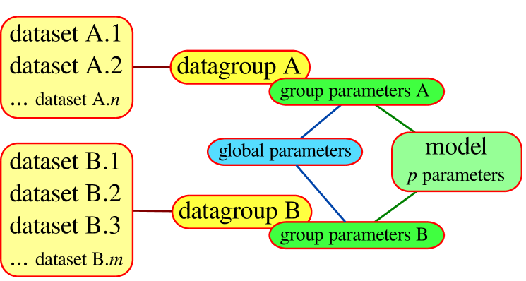
Figure 1: Terminology of simultaneous fits in ISIS. There are $n$ and $m$ simultaneous datasets, forming the datagroup A and B, respectively. Both datasets have their own group parameters, resulting from a model with $p$ parameters. Some of the group parameters are the same for both datagroups and are called global parameters.

Figure 1 illustrates these definitions. In this example, a dataset requires a model with $p$ parameters. There are simultaneous data from $n$ detectors available which can be described by the same parameters. These datasets define the datagroup A with $p$ free parameters. Another group of data was recorded by $m$ detectors. These datasets define an individual datagroup B with, again, $p$ free parameters. During the analysis of both groups, however, it turns out that a specific parameter seems to be equal for both data groups within the uncertainties. As a result, the two individual values for this parameter are tied to each other, resulting in a global parameter. That reduces the number of free parameters by one and the remaining group parameters can be constrained better.

2.2 Data- and analysis functions

Since simultaneous fits can have large numbers of fit parameters connected by a complicated logic, we provide a collection of all functions necessary to initialize and perform simultaneous fits in ISIS. The initialization of a simultaneous fit is performed via

 simfit = simultaneous_fit();

where simultaneous_fit returns a structure (Struct_Type), which has to be assigned to a variable, here simfit. The structure contains several functions and fields to handle simultaneous fits. The documentation of each function is available using the help-qualifier. Some important functions are described in the following.

 simfit.add_data(filenames);

This defines a datagroup and loads the spectra given by filenames, which must be an array of strings. The function also allows other data than spectra to be loaded or defined.

 simfit.fit_fun(model);

The string model defines the fit-function to be used for all datasets. Here, the placeholder % can be used instead of a component instance. In this case individual group parameters are applied to each datagroup automatically.

 simfit.set_par_fun(parameter, function);

This is probably one of the most useful functions. Like the ISIS intrinsic function, the value of the parameter is determined by the given function. The %-placeholder can be used within the string parameter to apply the function to the corresponding parameter of each data group. However, the function may contain other parameters or even a single parameter name as well. In the latter case, if the function is also applied to all datagroups (using the %), the single parameter is treated as global parameter from now on.

Because a simultaneous fit results in a large number of parameters, a single call to a fit-routine (fit_counts) will take a long time. In the example of the previous section, the final model fitted to the data consists of $(n+m)\times p$ parameters, where only $2p-1$ are free. To reduce the runtime of a fit, three fit-routines are implemented within the simultaneous- fit-structure.

 simfit.fit_groups(groupID);

Instead of perfoming a $\chi^{2}$-minimization of all parameters and datasets, this function loops over all datagroups and fits only the associated parameters (group parameters). If a group is specified by the optional groupID, then only the group parameters of this particular group are fitted.

 simfit.fit_global();

Instead of fitting the group parameters, this function fits the global parameters only. Since all defined data groups have to be taken into account, the fit usually takes longer than fitting the group parameters.

2.3 Uncertainty calculations

As already mentioned, the runtime of simultaneous fits is increased compared to fitting a single dataset only. Thus, uncertainty calculations of parameters, where a certain parameter’s range has to be found corresponding to a change in $\chi^{2}$, will be affected dramatically by the high runtime. Furthermore, it is necessary to distinguish between group- and global parameters. We recommend to compute the uncertainty intervals for each parameter on a different machine by, e.g., using [5] or mpi_fit_pars and the SLmpi module. We compared the runtime of a parallel uncertainty calculation in ISIS with a serial approach in XSPEC. Estimating the uncertainties of 10 parameters in parallel (i.e., on 10 cores) is faster by more than a factor of 3 (21 ks vs. 60 ks). Additionally, the calculations in ISIS resulted in a better $\chi^{2}_{\mathrm{red}}$ because the parameter ranges being scanned are larger in the parallel approach.

Group parameters depend on a single datagroup only. As a consequence, all other datagroups and therefore all other group parameters can be ignored during the uncertainty calculation. Unfortunately, that is not the case for global parameters. During the analysis of GRO J1008–57 (see Section 4), the uncertainties of the global parameters have been calculated by revealing the $\chi^{2}$-landscape of each global parameter by individual fits. Afterwards, every landscape has been interpolated to find the $\Delta\chi^{2}$-value of interest (e.g., $\Delta\chi^{2}=2.71$ corresponding to the 90%-confidence level). In this way the runtime of an uncertainty calculation of a single global parameter could be reduced significantly. Note that depending on the model and amount of data, such a computation can take up to several days.

3 Applications

There are various applications of simultaneous fits and data analysis. Besides determining specific parameters which seem to be constant over time by all available data, more physical questions can be tackled. For instance, if a physical property of the object of interest results in multiple observables:

• the geometry of the accretion column in accreting neutron star X-ray binaries affects the line shape of cyclotron resonant scattering features (CRSF) [6] as well as the pulse profile shape (Falkner et al., in prep.).

Furthermore, instead of deriving physical properties from parameters after fits have been performed, these properties can be directly fitted to the data by implementing the dependency on the model parameters:

• the components in radio maps of jets in active galactic nuclei move with certain velocities. Assuming a constant velocity of the jet components, the velocity itself could be a global fit parameter [7].

• in the sub-critical accretion regime of neutron stars, the spectrum is believed to harden with increasing luminosity [8]. Any possible dependency between power-law shape and luminosity could be fitted simultaneously with multiple spectra.

4 The Example GRO J1008–57

As an example of a successful simultaneous fit we briefly summarize the results of our analysis of GRO J1008–57 using almost all available X-ray spectra and -lightcurves. This transient high-mass X-ray binary consists of a neutron star orbiting a Be-type optical companion. For further details of the system as well as for the results of the analysis see [9] and references therein.

Since sources are only visible for a small fraction of their full orbit, it is challenging to obtain the orbital parameters of transient X-ray binaries by analyzing, e.g., pulse arrival times [10, 11]. Thus, an observed shift in the orbital phase with respect to initial orbital parameters can be fitted with either a different orbital period or time of periastron passage. This leads to a parameter degeneracy, which can be visualized by a contour map of the $\chi^{2}$-landscape of these parameters. The resulting contour map shows that both parameters are degenerated statistically (i.e., the ellipsoidal contour lines are tilted).

The outburst times of the source are, however, clearly connected to the periastron passage. Performing a simultaneous fit of the pulse arrival times and the outburst times reduces the parameter degeneracy and results in much better constrained parameters (about a factor of 2-3) as seen by recalculated contour map.

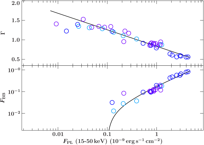
Figure 2: A fit (black lines) of the power-law index $\Gamma$ and black body flux $F_{\text{BB}}$ as functions of power-law flux $F_{\text{PL}}$. The different colors correspond to different outbursts.

Initial fits of the spectra of three outbursts of GRO J1008–57 in 2005, 2007 and 2011 with an absorbed cutoff power-law and an additional black body component showed that the folding energy $E_{\text{fold}}$, as well as the black body temperature $kT$, are independent of time within uncertainties. In particular, it seems that they do not change between different outbursts, i.e., these parameters are constant properties of the source.

Thus, those parameters are set as global parameters using simfit.set_par_fun and their values are determined by all available data. In addition, further parameters can be treated as global ones [see 9, for more details]. Finally, each observation is described by 3 group parameters only ($\approx$ degrees of freedom for each datagroup, the global parameters contribute marginally), which are the power-law flux $F_{\text{PL}}$, the black body flux $F_{\text{BB}}$, and the photon index $\Gamma$. The latter two strongly correlate with $F_{\text{PL}}$, but show no dependency on the outburst time or -shape. This correlation can be fitted to describe the spectrum of GRO J1008–57 by only one parameter: the power-law flux $F_{\text{PL}}$. The fit is shown in Fig. 2 and its values are given in Section 4.2 of [9].

As already mentioned in Section 2.3, the runtime of uncertainty calculations of the global parameters is increased dramatically. In the case of this analysis, the $\chi^{2}$-landscape produced by taking all 68 spectra into account was interpolated to estimate the uncertainties. The calculation of a single global parameter took $\sim\!7$ days on 100 CPUs (16320 CPUh).

5 Outlook

Although the simultaneous fits have already been applied successfully to real data (see Section 4 and [9]), the routines and functions are still under development. We recommend to pull the isisscripts-GIT-repository regularly to be up-to-date.

There are, however, some caveats according to Table 1 which one should be aware of (as with any routine, not just our ISIS implementation). In particular, the runtime still has to be reduced. One way to achieve this is by performing the fit on multiple CPUs, e.g., one CPU handles one dataset or datagroup. This has not been implemented yet because the dependencies of the datasets on each other require data exchange between the processes on the different machines. Additionally, the question about weighing the data is currently under discussion. The weight depends on the number of datapoints available in each dataset (or -group) as well as their uncertainties - but what does this mean for its importance, i.e., its effect on the model parameters? These remaining issues have to be clarified and the respective solutions will be published in the future.

- [1] J. C. Houck, et al. ISIS: An interactive spectral interpretation system for high resolution X-ray spectroscopy. In N. Manset, et al. (eds.), Astronomical Data Analysis Software and Systems IX, vol. 216 of Astron. Soc. of the Pacific Conf. Series, p. 591. 2000.
- [2] M. S. Noble, et al. Beyond xspec: Toward highly configurable astrophysical analysis. Publ of the Astron Soc of the Pacific 120:821–837, 2008.
- [3] R. A. Schafer. XSPEC, an X-ray spectral fitting package : version 2 of the user’s guide. European Space Agency, 1991.
- [4] K. A. Arnaud. Xspec: The first ten years. In G. H. Jacoby, et al. (eds.), Astronomical Data Analysis Software and Systems V, vol. 101 of Astron. Soc. of the Pacific Conf. Series, p. 17. 1996.
- [5] M. S. Noble, et al. Using the parallel virtual machine for everyday analysis. In C. Gabriel, et al. (eds.), Astronomical Data Analysis Software and Systems XV, vol. 351 of Astron. Soc. of the Pacific Conf. Series, p. 481. 2006.
- [6] G. Schönherr, et al. A model for cyclotron resonance scattering features. A&A 472:353–365, 2007.
- [7] C. Grossberger, et al. A&A In prep.
- [8] P. A. Becker, et al. Spectral formation in accreting X-ray pulsars: bimodal variation of the cyclotron energy with luminosity. A&A 544:A123, 2012.
- [9] M. Kühnel, et al. GRO J1008-57: an (almost) predictable transient X-ray binary. A&A 555:A95, 2013.
- [10] J. E. Deeter, et al. Pulse-timing observations of Hercules X-1. ApJ 247:1003–1012, 1981.
- [11] P. E. Boynton, et al. Vela X-1 pulse timing. I - determination of the neutron star orbit. ApJ 307:545–563, 1986.