Chimera patterns in the Kuramoto-Battogtokh model

Abstract

Kuramoto and Battogtokh [Nonlinear Phenom. Complex Syst. 5, 380 (2002)] discovered chimera states represented by stable coexisting synchrony and asynchrony domains in a lattice of coupled oscillators. After reformulation in terms of local order parameter, the problem can be reduced to partial differential equations. We find uniformly rotating periodic in space chimera patterns as solutions of a reversible ordinary differential equation, and demonstrate a plethora of such states. In the limit of neutral coupling they reduce to analytical solutions in form of one- and two-point chimera patterns as well as localized chimera solitons. Patterns at weakly attracting coupling are characterized by virtue of a perturbative approach. Stability analysis reveals that only simplest chimeras with one synchronous region are stable.

Chimera states in populations of coupled oscillators have attracted large interest since their first observation and theoretical explanation by Kuramoto and Battogtokh Kuramoto and Battogtokh (2002). The essence of chimera is in the spontaneous symmetry breaking: although a homogeneous fully symmetric synchronous state exists, yet another nontrivial state combining synchrony and asynchrony is possible and can even be stable. Chimeras can be found at interaction of several populations of oscillators Abrams et al. (2008); *Pikovsky-Rosenblum-08; *Tinsley_etal-12; *Martens_etal-13, or in an oscillatory medium Abrams and Strogatz (2004); Shima and Kuramoto (2004); Laing (2009); Bordyugov et al. (2010), the latter situation can be treated as a pattern formation problem. Here the formulation in terms of the coarse-grained complex order parameter indeed allows one to reduce the problem to that of evolution of a complex field Laing (2009); Bordyugov et al. (2010). For a recent review see Panaggio and Abrams (2015).

The goal of this paper is to develop a theory of chimera patterns in a one-dimensional (1D) medium based on formulation of the problem as a set of partial differential equations (PDEs). This allows us to represent the chimera state as a solution of ordinary differential equations (ODEs), periodic in space chimeras correspond to periodic orbits of these ODEs. We show that in a limit of neutral coupling, these equations are integrable yielding singular “one-point” and “two-point” chimeras; for a weakly attracting coupling we find properties of chimera patterns by virtue of perturbation analysis to these solutions. Furthermore, we study stability of found chimera patterns by employing a numerical method allowing to disentangle the essential continuous and the discrete (point) parts Wolfrum et al. (2011); Omel’chenko (2013) of the stability spectrum.

The original Kuramoto-Battogtokh (KB) model Kuramoto and Battogtokh (2002) is formulated as a 1D field of phase oscillators $\phi\left(x,t\right)$ evolving according to

$$\partial_{t}\phi=\omega+\mathrm{Im}\left(e^{-i\left(\phi+\alpha\right)}\!\int\!G\left(x-\tilde{x}\right)e^{i\phi(\tilde{x},t)}d\tilde{x}\right),$$ (1)

with exponential kernel $G\!\left(y\right)=\kappa\exp\bigl{(}-\kappa\left|y\right|\bigr{)}\!\bigl{/}2\bigr{.}$. Coupling is attractive if the phase shift $\alpha<\pi\bigl{/}2\bigr{.}$, then the synchronous state where all the phases are equal is stable; $\alpha=\pi\bigl{/}2\bigr{.}$ corresponds to neutral coupling.

One can reformulate this setup as a 1D continuous oscillatory medium Laing (2009); Bordyugov et al. (2010), described by the complex field $Z\!\left(x,t\right)$, which represents a coarse-grained order parameter of the phases: $Z\!\left(x,t\right)=\frac{1}{2\delta}\int_{x-\delta}^{x+\delta}e^{i\phi(\tilde{x},t)}d\tilde{x}$. In the synchronous state $|Z|=1$, while for partial synchrony $0<|Z|<1$. The dynamics of $Z\!\left(x,t\right)$ just follows locally the Ott-Antonsen equation Ott and Antonsen (2008); Panaggio and Abrams (2015)

$$\partial_{t}Z=i\omega Z+\bigl{(}e^{-i\alpha}H-e^{i\alpha}H^{\ast}Z^{2}\bigr{)}\bigl{/}2\bigr{.}\;.$$ (2)

where a field $H\!\left(x,t\right)\!=\!\int\!G\!\left(x-\tilde{x}\right)Z\!\left(\tilde{x},t\right)d\tilde{x}$ describes the force due to coupling. This nonlocal coupling according stems from the following model for the interaction of oscillators via the “auxiliary” field $H$ (cf. Refs. Shima and Kuramoto (2004); Laing (2011, 2015)):

$$\tau\partial_{t}H=\kappa^{-2}\partial^{2}_{xx}H-H+Z\;.$$ (3)

In the limit $\tau\to 0$, Eq. (3) reduces to an equation

$$\partial^{2}_{xx}H-\kappa^{2}H=-\kappa^{2}Z\;,$$ (4)

solution of which depends on boundary conditions. In particular, in an infinite medium $\left|x\right|<\infty$, the solution is $H\!\left(x,t\right)=\!\int\!\left(\kappa\exp\bigl{(}-\kappa\left|x-\tilde{x}\right|\bigr{)}\!\bigl{/}2\bigr{.}\right)Z\!\left(\tilde{x},t\right)d\tilde{x}$ as in (1).

Below we consider periodic in space medium with period $L$, in this case the KB model exactly corresponds to Eqs. (2), (4) if integration is performed in an infinite domain while the fields are assumed to have period $L$. If an integration over the periodic domain of size $L$ is performed, one should use the kernel

$$G(y)=\frac{\kappa}{2\sinh\bigl{(}\kappa L\bigl{/}2\bigr{.}\bigr{)}}\cosh\bigl{(}\kappa\left(\left|y\right|-L\bigl{/}2\bigr{.}\right)\bigr{)}\;,$$ (5)

which follows from the solution of (4) with periodic boundary conditions.

The formulated problem (2), (4) contains two parameters having dimension of length: $\kappa$ and $L$. By rescaling coordinate $x$ we can set one of these parameters to one. It is convenient to set $\kappa=1$, then the only parameter is the size of the system $L$.

Our next goal is to find chimera states, which consist of synchronous and asynchronous parts. We look for rotating-wave solutions of system (2), (4), which are stationary in a rotating reference frame: $Z(x,t)=z(x)e^{i(\omega+\Omega)t}$, $H(x,t)=h(x)e^{i(\omega+\Omega)t}$, where $\Omega$ is some unknown frequency to be defined below bib (a). Substituting this we get a system of an algebraic equation and an ODE for complex functions $z\!\left(x\right)$ and $h\!\left(x\right)$

$$e^{i\alpha}h^{\ast}z^{2}+2i\Omega z-e^{-i\alpha}h=0\;,$$ (6)

$$h^{\prime\prime}-h=-z\;.$$ (7)

Here and below prime denotes spatial derivative.

The first step is to express $z\!\left(x\right)$ from the quadratic equation (6) (see bib (b)). This equation describes the order parameter $z\!\left(x\right)$ of a set of oscillators driven by field $h\!\left(x\right)=r\!\left(x\right)e^{i\theta\left(x\right)}$, the solution at each point $x$ depends on the relation between $r$ and $\Omega$ (below for simplicity of presentation we write the relations for $\Omega<0$). If $\left|r\right|\geq\left|\Omega\right|$, then the oscillators are locked and $|z|=1$, otherwise the oscillators are partially synchronous with $0<|z|<1$. The solution reads

$$z\!=\!\begin{cases}-\left(i\Omega-\sqrt{r^{2}\!-\!\Omega^{2}}\right)r^{-1}e^{i(\theta-\alpha)},\hskip 5.69054pt\text{if}\hskip 5.69054pt\left|r\right|\!\geq\!\left|\Omega\right|,\vspace{1.0mm}\\ -i\left(\Omega+\sqrt{\Omega^{2}\!-\!r^{2}}\right)r^{-1}e^{i(\theta-\alpha)},\hskip 5.69054pt\text{if}\hskip 5.69054pt\left|r\right|\!<\!\left|\Omega\right|.\end{cases}$$ (8)

We now substitute this solution in (7). Although $h\!\left(x\right)$ is complex, the resulting equation can be written, due to gauge invariance $\theta\!\left(x\right)\!\to\!\theta\!\left(x\right)+\theta_{0}$, as a third-order system of ODEs for real functions $r\left(x\right)$ and $q\left(x\right)\!=\!r^{2}\left(x\right)\theta^{\prime}\left(x\right)$

$$r^{\prime\prime} =r+r^{-3}q^{2}\!-r^{-1}\sqrt{r^{2}-\Omega^{2}}\cos\alpha+r^{-1}\Omega\sin\alpha\;,$$ (9)

$$q^{\prime} =\Omega\cos\alpha+\sqrt{r^{2}-\Omega^{2}}\sin\alpha\;,$$

in the domain where $\left|r\right|\!\geq\!\left|\Omega\right|$, and

$$r^{\prime\prime} =r+r^{-3}q^{2}+r^{-1}(\Omega+\sqrt{\Omega^{2}-r^{2}})\sin\alpha\;,$$ (10)

$$q^{\prime} =(\Omega+\sqrt{\Omega^{2}-r^{2}})\cos\alpha\;,$$

in the domain where $\left|r\right|\!<\!\left|\Omega\right|$.

Our goal is to find chimera patterns described by equations (9), (10), satisfying periodicity condition $r(x+L)=r(x)$, $q(x+L)=q(x)$. It is more convenient not to fix the period $L$, but to fix the frequency of the rotating chimera $\Omega$, then to find periodic solutions of (9), (10), period $L$ of which depends on $\Omega$ (see bib (b)). This will after inversion yield dependence $\Omega(L)$.

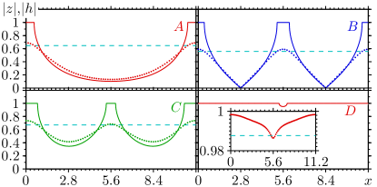
Figure 1: (Color online) Profiles of simplest chimeras (with at most two SRs) for $\alpha\!=\!1.457$, $|z|$: solid lines, $|h|$: dotted lines. $A$: the KB one-SR chimera for $\Omega\!=\!-0.648$, $B$: symmetric two-SRs chimera for $\Omega\!=\!-0.558$, $C$: asymmetric two-SRs chimera (here the widths of synchronous domains are different, and their phases differ not by $\pi$, like in case $B$) for $\Omega\!=\!-0.672$, $D$: nearly synchronous one-SR chimera for $\Omega\!=\!-0.98762$. Colors used correspond to coding of solutions in Fig. 3.

Before discussing numerical and analytical approaches, we illustrate in Fig. 1 several solutions for $\alpha=1.457$ (the value used in Kuramoto and Battogtokh (2002)) with period $L\approx 11.2$. Presented solutions (types $A$ and $B$ have been already discussed in the literature Kuramoto and Battogtokh (2002); Omel’chenko (2013); Panaggio and Abrams (2015)) are just simplest possible chimeras with at most two synchronous regions (SRs). Indeed, the system (9), (10) is a reversible (with respect to involution $r\to r$, $q\to-q$) third-order system of ODEs with a plethora of solutions, including chaotic ones. We illustrate this by constructing a two-dimensional Poincaré map in Fig. 2a. It shows typical for nearly integrable Hamiltonian systems picture of tori and periodic orbits of different periods. Not all points on the Poincaré surface lead to physically meaningful solutions: we discarded the trajectories which resulted in values $\left|r\right|\!>\!1$. The fixed point of the map Fig. 2(a) at $q=0$, $r\approx 0.84$ describes the one-hump chimera state $A$ in Fig. 1. The Poincaré map is constructed for a fixed value of $\Omega$, it provides several branches of periodic orbits having different periods. Collecting solutions at a fixed period $L$, we obtain are many coexisting chimera patterns; several three-SRs chimeras are illustrated in Fig. 2b. Our aim in this study is not to follow all possible periodic and chaotic solutions of this reversible system, below we focus on the simplest ones illustrated in Fig. 1, corresponding to fixed points and period-two orbits of the Poincaré map.

Figure 2: (Color online) (a) Poincaré map for system (9), (10) for $\alpha=1.457$ and $\Omega=-0.8$. The condition for the section: $r^{\prime}=0$, $r^{\prime\prime}<0$. (b) More complex patterns with three SRs for $L\approx 15.1$ and $\Omega=-0.796$ (solid red line), $\Omega=-0.726$ (dashed blue line) and $\Omega=-0.674$ (dotted black line).

Remarkably, it is possible to describe basic chimera profiles semi-analytically, for $\alpha\approx\pi\bigl{/}2\bigr{.}$. Let us first consider the limiting case $\alpha=\pi\bigl{/}2\bigr{.}$. Here, according to (9), (10), the derivative $q^{\prime}\!\left(x\right)$ is non-negative in the synchronous state and vanishes in the asynchronous state. Thus, a periodic solution with $q(x)=q(x+L)$ should be everywhere asynchronous, except possibly for one or two points at which $r(x)$ achieves an extremum $|r|=|\Omega|$. For this degenerate chimera Eqs. (10) reduce to $q=0$ and an integrable second-order equation

$$\begin{gathered}r^{\prime\prime}=-dU(r)\bigl{/}dr\bigr{.}\;,\\ U(r)=-r^{2}\bigl{/}2\bigr{.}-\sqrt{\Omega^{2}\!-\!r^{2}}-\Omega\ln\!\left(\sqrt{\Omega^{2}\!-\!r^{2}}\!-\!\Omega\right).\end{gathered}$$ (11)

In the potential $U\!\left(r\right)$, there are two types of trajectories, having maximum at $r_{max}=|\Omega|$, depending on the value of $\Omega$. For $-1<\Omega<\Omega_{\ast}=2\left(\ln 2-1\right)$ this is a periodic orbit with $0<r_{min}\leq|\Omega|$. It reaches the boundary of the asynchronous region at one point and corresponds to “one-point chimera”, which can be considered as the limiting case of curve $A$ in Fig. 1, where the SR shrinks to a point. For $\Omega_{\ast}<\Omega<0$ there is a symmetric periodic orbit (here it is convenient to allow $r$ to change sign, this corresponds to a jump by $\pi$ in phase $\theta$ if $r$ is considered as positive like in Fig. 1, curve $B$) with $-|\Omega|\leq r\leq|\Omega|$. This “two-point chimera” corresponds to curve $B$ in Fig. 1. These two types of solutions merge in a homoclinic orbit with infinite period at $\Omega=\Omega_{\ast}$, which can be named “chimera soliton” (one- or two-point, depending on which side of the threshold the orbit is considered). The dependencies $\Omega\!\left(L\right)$ for these solutions are shown in Fig. 3 as solid lines. Note that, additionally, there is a branch of synchronous solutions with $\Omega=-1$ which are steady states $r=1$.

The solutions above are degenerate chimeras, as the SR is restricted to one or two points. Synchronous region becomes finite for $\alpha\lesssim\pi\bigl{/}2\bigr{.}$, here one can develop a perturbation approach by introducing a small parameter $\beta=\pi\bigl{/}2\bigr{.}-\alpha\ll 1$. Now $q\neq 0$, but because $q\sim\beta$, we can neglect terms $\sim q^{2}$ in (9), (10). Then, the problem reduces to finding a periodic trajectory $r(x)$ of integrable equation, such that evolution of $q(x)$ is periodic:

$$\begin{gathered}\oint\!q^{\prime}\!\left(x\right)dx\!=\!\!\int_{x:\,\left|r\left(x\right)\right|\geq\left|\Omega\right|}\!\left(\Omega\beta\!+\!\sqrt{r(x)^{2}\!-\!\Omega^{2}}\right)dx+{}\\ {}\hskip 41.25648pt\int_{x:\,\left|r\left(x\right)\right|\geq\left|\Omega\right|}\!\beta\!\left(\Omega\!+\!\sqrt{\Omega^{2}\!-\!r^{2}\!\left(x\right)}\right)dx\!=\!0\;.\end{gathered}$$ (12)

Detailed calculations are presented in bib (b). The result is that the size $L_{syn}$ of SR becomes finite:

$$L_{syn}\approx\sqrt{\frac{8\beta}{\pi N_{SR}\sqrt{|\Omega|(1-|\Omega|)}}\oint\!\left(R^{\prime 2}+R^{2}\right)dx}\;.$$ (13)

where $R(x)$ is the solution of (11) at $\beta=0$ and $N_{SR}$ is the number of SRs.

We compare the analytical approach above with the results of direct numerical calculation, in the framework of (9), (10), of periodic orbits in Fig. 3, for several values of $\alpha$. Panel (a) shows that for small $\beta$ chimera states (of types $A$ and $B$ of Fig. 1) are close to degenerate regimes at $\beta=0$. One can see in panels (a,b) that the two analytic solutions at $\alpha=\pi\bigl{/}2\bigr{.}$ (the one-point chimera and the synchronous state) merge into one branch at $\alpha\lesssim\pi\bigl{/}2\bigr{.}$ with a nonmonotonous dependence $\Omega$ on $L$, cf. one-SR chimeras $A$ and $D$ in Fig. 1. In panel (b) one can see an additional branch corresponding to the two-SRs asymmetric chimera $C$ in Fig. 1. As a result, in (b) and (c) one has four solutions in some range of periods $L$. Only two of them survive for small $\alpha$; diagrams for $\alpha<0.9$ are qualitatively the same as panel (d) in Fig. 3.

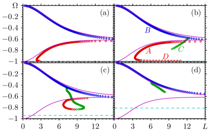
Figure 3: (Color online) Periods of chimera states $L$ vs. parameter $\Omega$ for $\alpha=1.514$ (a), $\alpha=1.457$ (b), $\alpha=1.229$ (c), and $\alpha=0.944$ (d). Chimera states for $\alpha=\pi\bigl{/}2\bigr{.}$, obtained by integration Eq. (11), are shown with violet solid lines. Different markers correspond to chimera types depicted in Fig. 1, as specified in panel (b). Cyan dashed lines show frequency of the synchronous state $\Omega=-\sin\alpha$.

Next, we discussed stability of the obtained chimera patterns. For this goal we linearize Eq. (2), (5) (see bib (b)). Contrary to the problem of finding chimera solutions, this analysis cannot be reduced to that of differential equations, rather we have to consider an integral-differential equation (2), (5) for $Z(x,t)$. After spatial discretization we get a matrix eigenvalue problem. The difficulty here is that, according to Omel’chenko (2013); Xie et al. (2014), there is an essential continuous $T$-shaped spectrum $\lambda_{c}$ consisting of eigenvalues on the imaginary and the negative real axis, but stability is determined by the point spectrum $\lambda_{p}$. Unfortunately, it is not easy to discriminate these parts of the spectrum in the eigenvalues $\lambda$ of the approximate matrix, because the eigenvalues representing essential part of spectrum lie not exactly on the imaginary axis. We adopted the following procedure to select the point spectrum $\lambda_{p}$. For a chimera state in the domain $0\leq x\leq L$, we can discretize the linearized system by using a set of points $x_{0}+j\Delta$, $j=0,1,\ldots,M-1$, where $\Delta=L/M$ and $0\leq x_{0}\leq\Delta$ is an arbitrary continuous parameter. This leads to an $2M\times 2M$ real matrix, eigenvalues $\lambda$ of which we obtained numerically. Additionally, we varied the offset of discretization $x_{0}$. In numerics we used $M=2048$ and $N=64$ or $N=128$ equidistant values of $x_{0}$. We have found that while the components of the essential spectrum vary with $x_{0}$, the point spectrum $\lambda_{p}$ components vary extremely weakly with $x_{0}$ – this allowed us to determine point spectrum $\lambda_{p}$ reliably for most values of parameters.

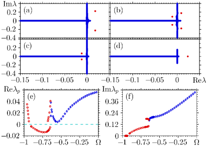
Figure 4: (Color online) (a-d): Essential (blue markers) and point (red markers) spectra for chimera states at $\alpha=1.457$ and four values of $\Omega$: (a) $\Omega=0.45$, (b) $\Omega=0.675$, (c) $\Omega=0.8$, (d) $\Omega=0.95$. In these plots all $2MN$ eigenvalues with $M=2048$ and $N=128$ are plotted. (e,f): real and imaginary parts of point spectrum $\lambda_{p}$ for solutions $A,D$ (red circles) and $B$ (blue diamonds) of Fig. 3(b).

Below we present stability analysis for $\alpha=1.457$, for branches $A,B,C,D$ (see Fig. 3(b)). Four characteristic types of spectra are shown in Fig. 4(a-d). Only case (c) with point spectrum $\lambda_{p}$ having negative real part corresponds to a stable chimera pattern, while all other patterns are unstable (oscillatory instability for cases (a,b) and monotonous instability for case (d)). Dependence of the point spectrum $\lambda_{p}$ on parameter $\Omega$ for $\alpha=1.457$, branches $A,B,D$, is shown in Fig. 4(e,f). One can see that in the region $-0.68\lesssim\Omega\lesssim-0.64$ there are four points of $\lambda_{p}$, for other values of $\Omega$ there is only one pair of eigenvalues (or one real eigenvalue for branch $D$). This property may be attributed to the fact, that close to the homoclinic orbit $\Omega\approx\Omega_{\ast}$ the length of the patterns is large so here two discrete modes are possible. The only stable chimera state is of type $A$ (we refer here to Figs. 1 and 3(b)) with $-0.91\lesssim\Omega\lesssim-0.69$. On the contrary, chimera states with two SRs (type $B$) are unstable. Most difficult was analysis of two-SRs solutions of type $C$ (Fig. 5), here the unstable branch of point spectrum $\lambda_{p}$ is real, and there is up to three stable complex pairs. In some cases only very fine discretization with $M=6144$ allowed us to reveal unstable point eigenvalues $\lambda_{p}$; we attribute this to a complex profile of this solution, requiring high resolution of perturbations.

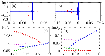
Figure 5: (Color online) All eigenvalues [(a): $\Omega=-0.645$, (b): $\Omega=-0.735$, here $M=4096$, $N=64$] and point spectra in dependence on $\Omega$ (c,d) for the asymmetric branch $C$.

Stability properties have been confirmed by direct numerical simulations of the ensemble governed by Eq. (1), (5), see Fig. 6 for space-time plots of field $|H(k,t)|=|\sum_{j}G(|k-j|/KL)\exp[i\phi_{j}]|$. One can initialize all the chimera patterns found above; in the unstable regions these patterns are destroyed, while stable chimera persists. Remarkably, for weakly unstable two-SRs chimeras for $\Omega\approx-0.58$, where the real part of the point eigenvalue $\lambda_{p}$ has a minimum (see Fig. 4(e)), the life time of prepared chimera is relatively large.

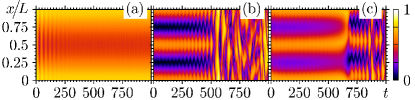
Figure 6: (Color online) Direct numerical simulations of stable and unstable chimeras for $\alpha\!=\!1.457$. (a): Chimera of type $A$ for $\Omega=-0.71377$, $L=6.03$; (b): chimera of type $B$ for $\Omega=-0.575$, $L=12.06$; (c): chimera of type C, $\Omega=-0.6$, $L\!=\!12.06$. The number of oscillators was $K\!=\!700$ per length unit.

Summarizing, in this Letter we reformulated the problem of chimera patterns in 1D medium of coupled oscillators as a system of PDEs. This allowed to find uniformly rotating chimera states as solutions of an ODE. Although a large variety of patterns with large spatial periods can be found, we restricted our attention in this Letter to the simplest ones, with at most two synchronous domains. Remarkably, these profiles can be explicitly described in the limit of neutral coupling between oscillators; for coupling close to neutral one, a perturbation analysis yields approximate solutions. Exploring stability of the found solutions appeared to be a nontrivial numerical problem. We suggested an approach to characterize the essential and the point parts of the spectrum via finite discretizations. It appears that only chimeras of the type originally studied by Kuramoto and Battogtokh are stable, while other found patterns are linearly unstable.

The approach suggested could be extended in several directions. First, one can study general bifurcations of chimera patterns. The difficulty here is that many tools for bifurcation analysis require sufficient smoothness of the equations, what is not the case for chimera solutions. Stability analysis performed in this letter have been restricted to perturbations with the same spatial period as the chimera itself, i.e. it describes stability for a medium on a circle. Other unstable modes, e.g. of modulational instability type, could appear if one formulates the stability problem for an infinite medium. Finally, the formulated PDEs have been simplified using the separation of time scales; it would be interesting to study stability of chimeras in the full Eqs. (2), (3) with $\tau\neq 0$.