Quantal rotation and its coupling to intrinsic motion in nuclei

Abstract

Symmetry breaking is an importance concept in nuclear physics and other fields of physics. Self-consistent coupling between the mean-field potential and the single-particle motion is a key ingredient in the unified model of Bohr and Mottelson, which could lead to a deformed nucleus as a consequence of spontaneous breaking of the rotational symmetry. Some remarks on the finite-size quantum effects are given. In finite nuclei, the deformation inevitably introduces the rotation as a symmetry-restoring collective motion (Anderson-Nambu-Goldstone mode), and the rotation affects the intrinsic motion. In order to investigate the interplay between the rotational and intrinsic motions in a variety of collective phenomena, we use the cranking prescription together with the quasiparticle random phase approximation. At low spin, the coupling effect can be seen in the generalized intensity relation. A feasible quantization of the cranking model is presented, which provides a microscopic approach to the higher-order intensity relation. At high spin, the semiclassical cranking prescription works well. We discuss properties of collective vibrational motions under rapid rotation and/or large deformation. The superdeformed shell structure plays a key role in emergence of a new soft mode which could lead to instability toward the $K^{\pi}=1^{-}$ octupole shape. A wobbling mode of excitation, which is a clear signature of the triaxiality, is discussed in terms of a microscopic point of view. A crucial role played by the quasiparticle alignment is presented.

• February 2014

1 Introduction

There are a variety of rotating objects in the universe. We are living on the rotating earth which is revolving around the sun. The sun is a part of our rotating galaxy. The neutron star is often observed as a “pulsar” whose rotational period can be as small as $10^{-3}$ s. However, if we look into a microscopic world, we find much faster rotating objects, such as nuclei. The nuclear rotational period in heavy nuclei is typically $\tau_{\rm rot}=10^{-19}\sim 10^{-20}$ s. This time scale is $100-1,000$ times larger than the period of the single-particle Fermi motion inside the nucleus, $\tau_{F}\sim 10^{-22}$ s. Thus, the rotational motion can be treated as “slow” motion at low-spin states. However, in high-spin states produced by the fusion reaction, it could reach $\tau=10^{-21}\sim 10^{-22}$ s which is comparable to $\tau_{F}$. Therefore, the nuclei provide a unique laboratory to study rapidly rotating quantum systems under strong Coriolis and centrifugal fields.

The nucleus is a finite quantum many-body system. Since the Hamiltonian is rotationally invariant, its energy eigenstate has a definite total angular momentum $I$. In order to realize the nuclear rotation, the nucleus needs to define its orientation. Since it is impossible to do it for spherical systems, a deformed intrinsic state, which is produced by breaking the rotational symmetry, is necessary. The word “intrinsic” means the degrees of freedom approximately independent of the rotational motion. The spontaneous breaking of symmetry (SBS) is an important concept to constitute the unified model of Bohr and Mottelson [1]. Hereafter, we denote the textbook [1] by “BM2”.

The SBS is strictly defined only in infinite systems. Therefore, in the beginning of this article (sections 2, 3, and 4), we address the following basic questions.

1. What is the origin of nuclear deformation?

2. What is the meaning of the SBS in finite systems?

3. What kind of collective motion will emerge due to the SBS?

These are important issues to understand the essence of the nuclear structure physics. We hope that these sections are useful, especially for students and non-practitioners.

The rotational motion is a collective motion emerged from the SBS, corresponding to the massless Anderson-Nambu-Goldstone (ANG) mode [2, 3, 4, 5, 6, 7] in the infinite system. It is approximately decoupled from the intrinsic motions, however, the decoupling is never exact. Moreover, as we mentioned in the beginning, we may generate a nucleus spinning extremely fast in experiments. Coupling between the rotational and intrinsic motions produces a variety of phenomena. We will discuss several related topics in sections 5, 6, and 7.

The coupling introduces the Coriolis mixing among different bands. The angular momentum dependence ($I$-dependence) of the transition matrix elements is very sensitive to this, even at low spin. The unified model predicts a form of the $I$-dependent intensity relation, however, a systematic way of calculating intrinsic moments entering in the intensity relation was missing. We present a feasible microscopic method for the calculation of the intrinsic moments using the cranking model at an infinitesimal rotational frequency (section 5).

Low-lying vibrational modes of excitation strongly reflect the underlying shell structure. Therefore, the new shell structure produced by rapid rotation and large deformation may significantly change their properties, and could lead to new soft modes and instability. Octupole vibrations at large angular momentum and in superdeformed bands are discussed. We present a possible banana-shaped superdeformation as a consequence of the superdeformed shell structure (section 6).

Nuclear wobbling motion, predicted by Bohr and Mottelson (section 4-5 in BM2), has been observed in ¹⁶³Lu and neighboring nuclei. This mode corresponds to a non-uniform three-dimensional rotation and provides a clear signature of nuclear deformation without the axial symmetry. Microscopic analysis reveals an important role played by the quasiparticle alignment. In fact, without the alignment, the wobbling motion cannot exist in ¹⁶³Lu. These issues and precession motion of the high-$K$ isomers are discussed in section 7.

For most of these studies, we use the quasiparticle-random-phase approximation (QRPA) in the rotating shell model, which we have developed for studies of rapidly rotating nuclei [8, 9, 10, 11]. Further inclusion of the quasiparticle-vibration coupling has been carried out for odd nuclei [12, 13, 14]. The method is still very useful and illuminating to obtain insights into nuclear structure in extreme conditions. In the present article, we do not present details of the theoretical models. Instead, we would like to concentrate our discussion on basic concepts and emergent phenomena.

2 Unified model and spontaneous breaking of symmetry

The atom is a finite-size quantum system, composed of electrons bound by the Coulombic attraction of the central nucleus. The nucleus is also a quantum finite-size fermionic system composed of nucleons. In both systems, the independent-particle (single-particle) motion is a prominent feature which leads to the “shell model”. In the first order approximation, the constituent particles (electrons in the atom and nucleons in the nucleus) freely move in the confining potential. However, there is an obvious but important difference between the atom and the nucleus. Namely, the nuclear potential binding the nucleons is generated by the nucleons themselves.

The electrons in the atom are bound by the attractive Coulomb potential generated by the nucleus. This potential is spherical, $-Ze^{2}/r$, in the atomic scale ($r\sim$Å). Although the repulsive interaction creates correlations among the electrons, the strong attractive potential always produces a restoring force which favors the spherical shape. In contrast, the shape of the nuclear potential is determined by the shape of the nucleus itself. It is often referred to as “nuclear self-consistency”. Therefore, we expect that the nucleus may change its shape, much easier than the atomic case. In other words, the nucleus is rather “soft” and produces low-energy “slow” shape vibrations.

2.1 Unified model Hamiltonian

Bohr and Mottelson treated these shape degrees of freedom as collective variables $\alpha$ in addition to the single-particle degrees of freedom $\xi$. In general, the shape dynamics described by $\alpha$ is considerably slower than the single-particle motion. Thus, we could adopt a picture that the nucleons move in a one-body potential $V(\xi,\alpha)$ which is specified by the nuclear shape $\alpha$. The idea ends up with the unified-model Hamiltonian,

$$H=H_{\rm coll}(\alpha)+H_{\rm sp}(\xi)+H_{\rm int}(\xi,\alpha),$$ (1)

where $H_{\rm coll}$ is the collective Hamiltonian to describe the low-energy shape vibrations. $H_{\rm sp}$ corresponds to the single-particle (shell model) Hamiltonian at the spherical shape, $H_{\rm sp}(\xi)=T_{\rm kin}(\xi)+V(\xi,\alpha=0)$. $T_{\rm kin}$ is the kinetic energy term and the nuclear self-consistency requires the potential $V(\xi,\alpha)$ to vary with respect to the shape $\alpha$. The interaction between the collective and single-particle motions, given by the third term $H_{\rm int}(\xi,\alpha)$, is indispensable to take into account this important property of nuclear potential.

2.2 Symmetry breaking mechanism

The coupling term in equation (1) could lead the nucleus to deformation. This is associated with the SBS mechanism. To elucidate the idea, let us adopt a simple adiabatic (Born-Oppenheimer) approximation. First, we solve the eigenvalue problem for the Schrödinger equation for the variables $\xi$ with a fixed value of $\alpha$,

$$H_{\rm def}(\alpha)|{\phi_{n}(\alpha)}\rangle=\epsilon_{n}(\alpha)|{\phi_{n}(\alpha)}\rangle,$$ (2)

where $H_{\rm def}(\alpha)\equiv H_{\rm sp}+H_{\rm int}(\alpha)$. This gives the adiabatic collective Hamiltonian, $H_{\rm ad}^{(n)}(\alpha)=H_{\rm coll}(\alpha)+\epsilon_{n}(\alpha)$, for each intrinsic eigenstate $\phi_{n}(\xi;\alpha)\equiv\langle\xi|\phi_{n}(\alpha)\rangle$. $H_{\rm ad}^{(n)}$ is an effective Hamiltonian for the collective variables $\alpha$. The total wave function is given by a product of the intrinsic and the collective parts [15], $\Psi_{n}(\alpha,\xi)=\psi^{(n)}(\alpha)\phi_{n}(\xi;\alpha)$.

There are two possible mechanisms of the SBS in the unified model to realize the deformed ground state with $\alpha\neq 0$. When $\epsilon_{0}(\alpha)$ strongly favors the deformation, even if $H_{\rm coll}(\alpha)$ has the potential minimum at $\alpha=0$, the adiabatic potential in $H_{\rm ad}^{(0)}(\alpha)$ may have a deformed minimum. Apparently, this mechanism requires the deformation-driving nature of $H_{\rm int}(\xi,\alpha)$, which we call “coupling-driven mechanism”. On the other hand, there is another mechanism which can deform the nucleus even if the spherical shape ($\alpha=0$) is favored by the adiabatic ground state $\epsilon_{0}(\alpha)$. This is due to the additional coupling caused by the kinetic term of $H_{\rm coll}$; $T_{\rm kin}(\alpha)=-(1/2)B\partial_{\alpha}^{2}$. We adopt units of $\hbar=1$ throughout the present article. Roughly speaking, the SBS takes place when the level spacing in $\epsilon_{n}(\alpha)$ is smaller than the additional coupling. It is analogous to the Jahn-Teller effect in the molecular physics [16], which we call “degeneracy-driven mechanism”.

2.3 Degeneracy-driven SBS; diagonal approximation

In order to understand the degeneracy-driven mechanism, we make the argument simpler, neglecting the off-diagonal elements, $\langle{\phi_{n}(\alpha)}|T_{\rm kin}(\alpha)|{\phi_{0}(\alpha)}\rangle$ ($n\neq 0$). Integrating the intrinsic (single-particle) degrees $\xi$, the effective Hamiltonian for the collective variable $\alpha$ is obtained as

$$H_{\rm eff}^{(0)}(\alpha)=\langle{\phi_{0}(\alpha)}|H|{\phi_{0}(\alpha)}\rangle=H_{\rm coll}^{(0)}(\alpha)+\epsilon_{0}(\alpha)+\Phi_{0}(\alpha),$$ (3)

where $H_{\rm coll}^{(0)}$ is identical to $H_{\rm coll}$ except that its kinetic energy is modified into $T_{\rm kin}^{(0)}(\alpha)=-(1/2)B(\partial_{\alpha}+\langle\phi_{0}|\partial_{\alpha}\phi_{0}\rangle)^{2}$. This is equivalent to introduction of a “vector” potential [17], $A(\alpha)\equiv i\langle\phi_{0}|\partial_{\alpha}\phi_{0}\rangle$. If the coordinate $\alpha$ is one-dimensional, the “vector” potential $A(\alpha)$ can be eliminated by a gauge transformation, $\exp(i\int A(\alpha)d\alpha)$. However, the following “scalar” potential remains.

$$\Phi_{0}(\alpha) = \frac{1}{2}B\langle{\partial_{\alpha}\phi_{0}}|(1-|{\phi_{0}}\rangle\langle{\phi_{0}}|)|{\partial_{\alpha}\phi_{0}}\rangle=\frac{1}{2}B\sum_{n\neq 0}\langle\partial_{\alpha}\phi_{0}|\phi_{n}\rangle\langle\phi_{n}|\partial_{\alpha}\phi_{0}\rangle$$ (4)

$$= \frac{1}{2}B\sum_{n\neq 0}\left|\frac{\langle{\phi_{n}(\alpha)}|(\partial_{\alpha}H_{\rm def}(\alpha))|{\phi_{0}(\alpha)}\rangle}{\epsilon_{0}(\alpha)-\epsilon_{n}(\alpha)}\right|^{2}.$$

From equation (4), it is apparent that $\Phi_{0}(\alpha)$ is positive and becomes large where the adiabatic ground state is approximately degenerate in energy, $\epsilon_{0}\approx\epsilon_{n}$ ($n\neq 0$). When the spherical ground state ($\alpha=0$) shows degeneracy, it could be significantly unfavored by $\Phi_{0}(\alpha)$. The system tends to avoid the degenerate ground state, which leads to the SBS with nuclear deformation.

We would like to emphasize again that the coupling between the collective (shape) degrees of freedom $\alpha$ and the intrinsic (single-particle) motion $\xi$ is essential to produce the nuclear deformation. This is apparent for the coupling-driven mechanism, and is also true for the degeneracy-driven case. If the coupling term $H_{\rm int}(\xi,\alpha)$ is absent, the adiabatic states $\phi_{n}(\xi)$ are independent of $\alpha$, thus, produce no gauge potentials, $A(\alpha)=\Phi_{0}(\alpha)=0$. We also note here that the present argument on the degeneracy-driven (Jahn-Teller) mechanism explains why the instability of a spherical state occurs, but not what kind of deformation takes place. This will be discussed in sections 3.3 and 6.2.

2.4 Field coupling

The oscillation of the variable $\alpha$ correspond to the shape vibration. Thus, it can be quantized to a boson operator. In order to describe the vibrational motion associated with $\alpha$, we introduce a boson space with the $n$-phonon state $|{n}\rangle$. When $\alpha$ is small, we may linearize the coupling term in equation (1) with respect to $\alpha$ as

$$H_{\rm int}(\xi,\alpha)=-\kappa\alpha F(\xi),$$ (5)

where $\kappa$ is a coupling constant which depends on the normalization of $\alpha$ and $F$. If the operator $F$ is given, the normalization of $\alpha$ is usually chosen as follows. The action of the one-body operator $F$ on the ground state (a Slater determinant) produces many one-particle-one-hole states; $F|{\Phi_{0}}\rangle=\sum_{ph}|{\Phi_{ph}}\rangle\langle{\Phi_{ph}}|F|{\Phi_{0}}\rangle$. This is identified with the operation of $\alpha$ in the collective (boson) space:

$$\sum_{ph}|\langle{\Phi_{ph}}|F|{\Phi_{0}}\rangle|^{2}=|\langle{n=1}|\alpha|{n=0}\rangle|^{2}.$$ (6)

The coupling constant $\kappa$ can be also determined by this self-consistency. See chapter 6 of BM2 for details of the field coupling techniques.

If the matrix elements of $F$ are identical to those of $\alpha$ as in equation (6), the field coupling (5) can be interpreted as an residual two-body interaction

$$H_{\rm res}(\xi)=-\frac{1}{2}\kappa F^{2}.$$ (7)

This kind of separable effective interactions have been extensively adopted in nuclear structure studies. Among them, the most famous one is the pairing-plus-quadrupole model [18, 19, 20], which was originally proposed by Bohr, Mottelson, and their colleague. It represents two kinds of important low-energy correlations in nuclei; One is the quadrupole correlations, $F\sim r^{2}Y_{2\mu}$, which are inspired by existence of low-lying $2^{+}$ vibrational excitations in even-even nuclei. Another correlation is the pairing, $F\sim P+P^{\dagger}$ and $F\sim P-P^{\dagger}$ where $P$ is the pair annihilation operator. This is important in heavy nuclei in which the nuclear superfluidity associated with the pair condensation is well established [21]. We also adopt this separable form as a residual interaction for the QRPA calculations in sections 5, 6, and 7.

3 Finite-size effect

Nuclei on earth are of finite size ($R<10$ fm) with finite number of nucleons ($A<300$). Strictly speaking, the SBS in the ground state is realized in the infinite system. For finite systems, the quantum fluctuation associated with the zero-point motion restores the broken symmetry. Thus, the symmetry-broken state is not stable for finite systems, in a rigorous sense. However, the SBS is ubiquitous in macroscopic objects in nature, which are made of big but finite number of particles. Thus, everybody agrees that the zero-point motion to restore the symmetry can be safely neglected in the macroscopic number, say $A\sim 10^{23}$. Then, how about the case of $A\sim 200$?

3.1 Finite correlation time

Let us consider a deformed nucleus and the single-particle states $\phi_{i}^{0}$ in the deformed Nilsson potential. The deformed ground state is simply assumed to be a Slater determinant, $|{\Phi_{0}}\rangle\equiv\det\{\phi_{1}^{0}\phi_{2}^{0}\cdots\phi_{A}^{0}\}$. If we rotate the nucleus by angle $\theta$, we have a state $|{\Phi_{\theta}}\rangle=\det\{\phi_{1}^{\theta}\phi_{2}^{\theta}\cdots\phi_{A}^{\theta}\}$. where $\phi_{i}^{\theta}=\hat{R}(\theta)\phi_{i}^{0}$ with the rotation operator $\hat{R}(\theta)$. Each single-particle state $\phi_{i}^{\theta}$ in the tilted Nilsson potential can be expanded in terms of the untilted state $\phi_{i}^{0}$, as $\phi_{i}^{\theta}=\sum_{j}^{\infty}c_{ij}^{\theta}\phi_{j}^{0}$. When the angle $\theta$ is small, we can estimate the diagonal coefficients as $|c_{ii}|\sim 1-c|\theta|$ with $c>0$, and the off-diagonal ones ($i\neq j$) as $|c_{ij}|\sim O(\theta)$. As far as the nucleon number $A$ is finite, the tilted ground state $|{\Phi_{\theta}}\rangle$ can be written in terms of the untilted Nilsson basis, $\{\phi_{i}^{0}\}$. This is due to the fact that $|{\Phi_{0}}\rangle$ and $|{\Phi_{\theta}}\rangle$ belong to the same Hilbert space.

However, in the limit of $A\rightarrow\infty$, this is no longer true. The tilted ground state is expanded in terms of the untilted Slater determinants as

$$|{\Phi_{\theta}}\rangle=\det\{\phi_{1}^{\theta}\cdots\phi_{A}^{\theta}\}=\sum_{j_{1},\cdots,j_{A}}C_{j_{1}\cdots j_{A}}\det\{\phi_{j_{1}}^{0}\cdots\phi_{j_{A}}^{0}\},$$ (8)

where $C_{j_{1}j_{2}\cdots j_{A}}=c_{1j_{1}}c_{2j_{2}}\cdots c_{Aj_{A}}$. For a small value of $\theta$, the largest coefficient among $\{|C_{j_{1}\cdots j_{A}}|\}$ is apparently $|C_{1\cdots A}|$ whose absolute magnitude is $|C_{1\cdots A}|\sim(1-c|\theta|)^{A}$. Therefore, all the coefficients $C_{j_{1}\cdots j_{A}}$ vanish exponentially as functions of $A$. This means that $|{\Phi_{0}}\rangle$ and $|{\Phi_{\theta}}\rangle$ belong to different Hilbert spaces at $A\rightarrow\infty$, thus, $|{\Phi_{\theta}}\rangle$ is no longer expandable in terms of the untilted Slater determinants. In other words, the deformed infinite nucleus never rotates.

The same issue can be examined in terms of the excitation spectra. The rotational spectra of deformed nuclei show $E_{I}=I(I+1)/2{\cal J}$, in which the moment of inertia $\mathcal{J}$ is approximately order of $A^{5/3}$. The rotational motion is quantized due to the finiteness of ${\cal J}$. In the limit of $A\rightarrow\infty$, the excitation spectra becomes gapless and the ground state ($I=0$) is degenerate with other states ($I\neq 0$). Therefore, an infinitesimally weak external field can fix its orientation by superposing states with different $I$.

Now, let us come back to the question, ”how about heavy deformed nuclei?”. As far as $A$ is finite, the “tilted” and “untilted” Hilbert spaces are equivalent. The zero-point fluctuation may connect $|{\Phi_{0}}\rangle$ and $|{\Phi_{\theta}}\rangle$, thus, the wave packet $|{\Phi_{0}}\rangle$ loses its direction in finite correlation time. If this time scale is significantly larger than that of the single-particle motion $\tau_{F}\sim 10^{-22}$ s, we can claim that the SBS takes place and the nucleus is deformed. In fact, this condition is well satisfied for heavy nuclei. Let us limit the orientation of the deformed nucleus to an angle range of unity ($\Delta\theta\sim 1$), then, the quantum fluctuation produces the angular momentum with the magnitude of $\Delta I\sim(\Delta\theta)^{-1}\sim 1$. This leads to the correlation time, $\tau_{\rm cor}\sim{\cal J}/\Delta I\sim{\cal J}$, that amounts to $10^{-19}$ s for typical deformed actinide nuclei. This argument is consistent with the vanishing behavior of the coefficients $C_{j_{1}\cdots j_{A}}$. Suppose the overlaps $|\langle\phi_{i}^{0}|\phi_{i}^{\theta}\rangle|\sim 0.9$ for $i=1,\cdots,A$, then, we have $C_{12\cdots A}\sim(0.9)^{A}\sim 7\times 10^{-10}$ for $A=200$. Therefore, the rotational fluctuation is significantly hindered for heavy deformed nuclei. These simple exercises also tell us that, the concept of SBS has a greater significance for nuclei with larger $A$ and larger deformation.

From a similar argument replacing the single-particle states $\phi_{i}^{0}$ in the Slater determinant $\det\{\phi_{j_{1}}^{0}\cdots\phi_{j_{A}}^{0}\}$ by those in a spherical potential, we may understand why the description based on the “symmetry-broken” deformed basis is important. It is apparent that, if we adopt a spherical shell model basis for such heavy well-deformed nuclei, we need to treat very small coefficients, $C_{j_{1}\cdots j_{A}}$, with enormous number of basis states. In the limit of $A\rightarrow\infty$, this treatment becomes impossible. The impossibility here is in a strict sense, not in a practical sense due to computational limitation. Thus, instead of superposing the “symmetry-preserving” (spherical) Slater determinants, the theories of restoring broken symmetry, such as the projection method, have been extensively developed in nuclear physics, to take into account effects of the zero-point fluctuation [22]. The usefulness of these symmetry restoration approaches has been recognized recently in other fields [23].

3.2 Zero-point motion and shell effect

As we have mentioned in section 3.1, the finiteness leads to the finite correlation time and the finite energy gap in the excitation spectra. In the symmetry restoration mechanism, the zero-point fluctuation associated with the ANG mode is a key element. In this subsection, we discuss effects of other zero-point motions in finite systems, which could hinder the SBS. The zero-point kinetic energy of nucleons is roughly given as $T_{\textrm{\sc zpe}}/A\sim 1/(mR^{2})\sim 10$ MeV. This is comparable to the nuclear binding energy $B/A\sim 8$ MeV and has a non-negligible effect. In fact, since the nucleons are fermions, the Fermi energy is even larger, $t_{F}\sim k_{F}^{2}/(2m)\sim 40$ MeV. The zero-point (Fermi motion) kinetic energy generally favors the “symmetry-preserving” state with a uniform and spherical density distribution. Since this competes with the SBS driving effect, the SBS which occurs in the thermodynamical limit may not occur in finite systems. The interplay between the zero-point motion and the interaction leads to interesting phenomena in nuclei.

The shell effect is a kind of finite-size effect in many fermion systems and is an indispensable factor in the low-energy nuclear structure. The prominent deformation hindrance effect can be found at the spherical magic numbers. The ground states of those magic nuclei favor spherical shape. Nevertheless, most of the spherical nuclei show the shape coexistence phenomena. For instance, the even-even spherical nuclei often have deformed excited $0^{+}$ states at very low energy. It is prevalent in many semi-magic nuclei, and even true for some doubly magic nuclei. In contrast, as far as we know, when the ground state is deformed, excited $0^{+}$ spherical states have not been clearly identified. In the Strutinsky shell correction method [24, 22], the shell effect is regarded as an origin of the nuclear deformation. It might be proper to say this in an opposite way; the heavy nuclei are “genetically” deformed, and some special nuclei become spherical because of the finite-size (spherical shell) effect to hinder the SBS.

3.3 Shell structure and soft modes

When the symmetry breaking takes place and the nucleus is deformed, what kind of shape is realized? This depends on the underlying shell structure. Let us present a simple argument based on the one given by by Bohr and Mottelson (pp. 578$-$591 in BM2). For a spin-independent spherical potential, the single-particle energy is characterized by the radial quantum number $n$ and the orbital angular momentum $l$, $\epsilon(n,l)$. When we change $n$ and $l$ from a certain value $(n_{0},l_{0})$.

$$\epsilon(n,l)=\epsilon(n_{0},l_{0})+\Delta n\left(\frac{\partial\epsilon}{\partial n}\right)_{0}+\Delta l\left(\frac{\partial\epsilon}{\partial l}\right)_{0}+\cdots,$$ (9)

where $\Delta n=n-n_{0}$ and $\Delta l=l-l_{0}$. Since $n$ and $l$ take only integer numbers, the ratio, $a:b\equiv({\partial\epsilon}/{\partial n})_{0}:({\partial\epsilon}/{\partial l})_{0}$ plays a very important role. If the ratio $a:b$ is rational, we can choose $a$ and $b$ as the integer numbers. Then, in the linear order (9), $\epsilon(n,l)$ and $\epsilon(n\pm mb,l\mp ma)$ are degenerate, where $m$ is an integer number.

Now, let us define the shell frequency as

$$\omega_{\rm sh}\equiv\frac{1}{a}\left(\frac{\partial\epsilon}{\partial n}\right)_{0}=\frac{1}{b}\left(\frac{\partial\epsilon}{\partial l}\right)_{0}.$$ (10)

There are degenerate single-particle energies at intervals of $\omega_{\rm sh}$. Larger integers $a$ and $b$ correspond to a smaller $\omega_{\rm sh}$. Therefore, the prominent shell structure with a large shell gap $\omega_{\rm sh}$ should be associated with the small integers $(a,b)$. For instance, the isotropic harmonic oscillator potential has the $a:b=2:1$ shell structure, with the constant $\omega_{\rm sh}$. The Coulomb potential has the strict $a:b=1:1$, with the energy-dependent $\omega_{\rm sh}$. In general, the degeneracy is approximate and the ratio $a:b$ may change according to the location of the Fermi level.

The derivatives, $(\partial\epsilon/\partial n,\partial\epsilon/\partial l)$, correspond to the (angular) frequencies in the classical mechanics; $\partial\epsilon/\partial n$ is the frequency of the radial motion, while $\partial\epsilon/\partial l$ is that of the angular motion. The integer ratio $(a,b)$ of the frequencies means that the classical orbit is closed (periodic). Therefore, the quantum shell structure is closely related to the classical periodic orbits.

Since the nuclear potential somewhat resembles the harmonic oscillator potential, the shell structure associated with $a:b=2:1$ is prominent. The $2:1$ periodic orbit in the harmonic oscillator potential is the elliptical orbit. When there are many valence nucleons in the degenerate levels, the short-range attractive interaction favors their maximal overlap, which eventually leads to the SBS to an ellipsoidal (quadrupole) shape. In the quantum mechanical terminology, we may say that the coupling among the degenerate single-particle levels with $\Delta l=2$ produces a soft mode. If the number of valence nucleons becomes large, this correlation may produce the quadrupole deformation.

The spin-orbit potential decreases the frequency $\partial\epsilon/\partial l$ for the single-particle levels of $j=l+1/2$. This could lead to a new shell structure of $a:b=3:1$ among the levels of the $j=l+1/2$. The $3:1$ frequency ratio corresponds to classical periodic orbits of the triangular shape, since the radial motion oscillates three times during the single circular motion. Thus, for heavy nuclei in which the high-$j$ single-particle levels ($j=l+1/2$) are located near the Fermi level, the approximate degeneracy of the $\Delta l=3$ levels may result in the octupole instability in open-shell configurations. For example, the neutron-deficient actinide nuclei show typical spectra of the alternating parity band, which are understood as a realization of the pear-shaped deformation of $Y_{30}$ type [25].

The investigation of the classical periodic orbits is useful to identify a soft mode and a favorable shape. The SBS toward the quadrupole deformation in open-shell nuclei is nicely explained in this simple argument. However, it is more difficult to explain the fact that most nuclei have the prolate shape, not the oblate shape. There have been a number of works on this issue [26, 27, 28, 29]. According to the classical periodic orbits, a recent analysis sheds new light on the prolate dominance in nuclei [30].

3.4 Fermi motion and nuclear self-consistency

In nuclei, the kinetic energy of nucleons’ Fermi motion is very large. Adopting the harmonic oscillator potential model, a simple estimate of the total kinetic energy is given by

$$T_{0}=\frac{1}{2}E_{\rm HO}=\frac{1}{2}\sum_{k=x,y,z}\omega_{k}\Sigma_{k},\quad\quad\Sigma_{k}\equiv\sum_{i=1}^{A}(n_{k}+\frac{1}{2})_{i},$$ (11)

where $n_{k}$ ($k=x,y,z$) are the oscillator quantum numbers of the single-particle states. For a spherical nucleus ($\omega_{x}=\omega_{y}=\omega_{z}=\omega_{0}$) filling the levels up to $n_{x}+n_{y}+n_{z}=N_{\rm max}$, this amounts to

$$T_{0}=(1/4)\omega_{0}(N_{\rm max}+1)(N_{\rm max}+2)^{2}(N_{\rm max}+3).$$ (12)

Taking $Z=N=40$ (⁸⁰Zr, $N_{\rm max}=3$), this gives $T_{0}=150\omega_{0}\sim 1.43$ GeV, with a standard value of $\omega_{0}\approx 41$A${}^{-1/3}\sim 9.5$ MeV. If we deform the harmonic oscillator to a prolate/oblate shape with $(\omega_{x},\omega_{y},\omega_{z})=(e^{\eta},e^{\eta},e^{-2\eta})\omega_{0}$, the kinetic energy becomes

$$T(\alpha)=\frac{2e^{\eta}+e^{-2\eta}}{3}T_{0},$$ (13)

which has the minimum value at the spherical shape $\eta=0$. According to equation (13), a moderate prolate deformation of $e^{\eta}=1.1$ will produce the increase in the kinetic energy by about 1 %. However, since $T_{0}$ is very large, this 1 % increase is significant, such as 14 MeV for $Z=N=40$. However, the deformed ground state in ⁸⁰Zr is suggested by experiments observing a ground-state rotational band [31]. How does the nucleus compensate this large increase in kinetic energy?

The solution to this problem is again attributed to the nuclear self-consistency. In the harmonic oscillator model, the self-consistency condition, that the deformation of the potential is equal to that of the density distribution, can be simply expressed by equation (4-115) in BM2,

$$\omega_{x}\Sigma_{x}=\omega_{y}\Sigma_{y}=\omega_{z}\Sigma_{z}.$$ (14)

Namely, when the nuclear potential is deformed as $(\omega_{x},\omega_{y},\omega_{z})=(e^{\eta},e^{\eta},e^{-2\eta})\omega_{0}$, the configuration of the ground state should change accordingly, $(\Sigma_{x},\Sigma_{y},\Sigma_{z})=(e^{-\eta},e^{-\eta},e^{2\eta})\Sigma_{0}$. Since the momentum distribution in the harmonic oscillator potential model can be calculated as $\langle p_{k}^{2}\rangle=m\omega_{k}\Sigma_{k}$ ($k=x,y,z$), the self-consistency condition (14) means the isotropic momentum (velocity) distribution (no deformation in the Fermi sphere). In other words, the shape of the nucleus is specified by the minimization of the kinetic energy which is equal to the isotropic velocity distribution.

This indicates the importance of configuration rearrangements in low-energy collective dynamics. When the nuclear deformation is changed as $(\omega_{x},\omega_{y},\omega_{z})\rightarrow(e^{\eta}\omega_{x},e^{\eta^{\prime}}\omega_{y},e^{-\eta-\eta^{\prime}}\omega_{z})$, the configuration should follow as $(e^{-\eta}\Sigma_{x},e^{-\eta^{\prime}}\Sigma_{y},e^{\eta+\eta^{\prime}}\Sigma_{z})$, to keep the Fermi sphere spherical. In order to change the configuration, we need two-particle-two-hole excitations, to annihilate a time-reversal pair of nucleons in a certain single-particle orbit and create a pair in another orbit. Therefore, we expect that, during the shape evolution at low energy, the pairing interaction plays a dominant role in dynamical change of the configuration. This was supported by experimental data that the spontaneous fission life times of even-even nuclei are much shorter than those of odd and odd-odd nuclei [32].

According to the nuclear self-consistency, each configuration has its optimal shape. We may think about possibilities of realizing different shapes corresponding to different configurations in the same nucleus. This phenomenon is called “shape coexistence”. For instance, in the harmonic oscillator model of ⁸⁰Zr with $N=Z=40$, in addition to the spherical configuration ($\Sigma_{x}=\Sigma_{y}=\Sigma_{z}$, $\omega_{x}=\omega_{y}=\omega_{z}$), the self-consistency condition (14) is also satisfied with the superdeformed configuration ($2\Sigma_{x}=2\Sigma_{y}=\Sigma_{z}$, $\omega_{x}=\omega_{y}=2\omega_{z}$). In fact, the shape coexistence phenomena have been observed in many areas throughout the nuclear chart [33].

3.5 Fermi sphere in the rotating frame

This idea of the isotropic velocity distribution can be extended into the one in the rotating frame (p.79 in BM2). The local velocity in the rotating frame,

$$\vec{v}\equiv\vec{p}/m-(\vec{\omega}_{\rm rot}\times\vec{r}),$$ (15)

has an isotropic distribution $\rho_{\vec{r}}(v)$ at each $\vec{r}$. The isotropic velocity distribution means no net current relative to the rotating frame, which ends up with a rigid-body value for the moment of inertia. The deformed nucleus would have a rigid-body value of moment of inertia if the pairing correlations were absent.

The transformation from the laboratory frame to the rotating frame leads to the cranking Hamiltonian

$$H^{\prime}=H-\vec{\omega}_{\rm rot}\cdot\vec{J},$$ (16)

where $\vec{J}$ is the total angular momentum. The velocity-dependent terms (kinetic energy and the centrifugal potential) in the rotating frame can be written as $p^{2}/(2m)-\vec{\omega}_{\rm rot}\cdot(\vec{r}\times\vec{p})=mv^{2}/2-m(\vec{\omega}_{\rm rot}\times\vec{r})^{2}/2$ where $\vec{v}$ is given by equation (15). This confirms the $\vec{v}$-dependence in $H^{\prime}$ is isotropic ($\propto v^{2}$). This isotropic velocity distribution is still valid in rotating nuclei [34]. The cranking model (16) plays a key role in physics of high-spin nuclear structure (sections 5, 6, and 7).

4 SBS and collective motions

A broken continuous symmetry leads to the emergence of two types of collective excitations. One is the massless ANG mode and the other is the massive Higgs mode [35]. Therefore, properties of the collective motions significantly change before and after the SBS takes place. In nuclei, we can observe them in the excitation spectra. We can even see how the ANG and Higgs modes appear and evolve from soft modes.

4.1 Rotational motion; ANG mode

The ANG mode is a gapless (massless) mode in the infinite system. For the case of nuclear deformation, the ANG mode correspond to the rotational motion of the deformed nucleus. Because of the finiteness, the spectrum is not exactly gapless, however, shows a gradual emergence of the “quasi-degenerate” rotational spectra.

In Fig. 6-31 of BM2, a typical example for even-even Sm isotopes (^144-154Sm) is presented. The ¹⁴⁴Sm nucleus has the magic neutron number $N=82$. Its ground state ($0^{+}$) is spherical and the first excited state is located at excitation energy of 1.63 MeV. Keeping the proton number the same and increasing the neutron number two by two, we clearly observe the following:

1. The first $2^{+}$, $4^{+}$, $\cdots$ ($2I$) states lower their excitation energies. Eventually, a rotational band is formed to present the excitation spectra, $E_{I}\propto I(I+1)$.

2. The second $0^{+}$ and the second $2^{+}$ states lower their energies in the beginning. However, they stop decreasing at $N=88$ (¹⁵⁰Sm).

3. Additional rotational bands are formed on top of the second $0^{+}$ and $2^{+}$ states for $N\geq 90$ (^152,154Sm).

In ¹⁵⁴Sm, the excitation energy of the first $2^{+}$ state is only 82 keV. This is 1/20 of that in ¹⁴⁴Sm and we may say that it is approximately degenerate in the ground state. Moreover, there appear five members ($0^{+},\cdots,8^{+}$) of rotational bands below 1 MeV of excitation. It should be noted that similar phenomena are observed in many region of nuclear chart, when the neutron (proton) numbers are going away from the spherical magic number.

A regular pattern of rotational spectra allows us to distinguish the intrinsic excitations and the rotational motion. A rotational band is constructed based on each intrinsic excitation from the ground state. From these observation, we may think of the Hamiltonian subtracting the rotational energy, $H^{\prime}\equiv H-{\vec{J}^{2}}/(2{\cal J})$. $H^{\prime}$ conserves the rotational symmetry, however, the member of the rotational bands ($0^{+}$, $2^{+},\cdots$) will be degenerate in energy. Then, a deformed wave-packet state which violates the rotational symmetry becomes an eigenstate of the Hamiltonian $H^{\prime}$.

The number of activated rotational degrees of freedom depends on the nuclear shape. For axially symmetric spheroidal shape, there is no collective rotation around the symmetry axis. In other words, the angular momentum component along the symmetry axis (called $K$ quantum number in the following) is purely determined by the intrinsic motion. In this case, the two rotational axes perpendicular to the symmetry ($z$) axis are possible, but they are equivalent in the sense that they have equal moment of inertia, ${\cal J}_{x}={\cal J}_{y}$. In contrast, if the nucleus has an equilibrium shape away from the axial symmetry (triaxial shape), the collective rotations about three axes are all activated, and they can have different moments of inertia, ${\cal J}_{x}$, ${\cal J}_{y}$, and ${\cal J}_{z}$. We may expect that the rotational spectra become richer and more complex. The wobbling motion is known to be a typical mode of excitation in the triaxial nuclei, that will be discussed in section 7.

4.2 Beta and gamma vibrations; amplitude (Higgs) mode

The quadrupole ($\lambda=2$) vibrations produce $2^{+}$ excitations in spherical nuclei. When the SBS takes place to produce the prolate (spheroidal) ground state, among five $\alpha_{2\mu}$ ($\mu=-2,\cdots,2$), the two shape degrees ($\beta$ and $\gamma$) remain, and rest of the degrees of freedom are absorbed in the rotational motion (Euler angle $\Theta$). For an axially symmetric ground state, the normal modes can be classified by the vibrational angular momentum along the symmetry axis, which is often denoted by the quantum number $K$. The $\beta$ and $\gamma$ vibrations correspond to $K^{\pi}=0^{+}$ and $2^{+}$, respectively. Note that the $K^{\pi}=1^{+}$ low-lying vibration does not exist, because it corresponds to the rotation of the whole nucleus.

The $\beta$ vibration around the SBS minimum is associated with a collective amplitude mode of order parameter with a finite energy gap, in contrast to the “gapless” rotational motion. This type of excitation is often referred to as the “amplitude (Higgs) mode” [35]. A number of those candidates have been observed in well-known deformed regions, such as the rare-earth and actinide regions. For instance, in the rare-earth region, the excitation energies of $\beta$ vibration candidates are found at $E_{x}\approx 1$ MeV. However, their $B(E2)$ values from the ground states to the $2^{+}$ states in the $\beta$-vibrational bands are not large in most cases, typically a few Weisskopf units. Instead, strong population by the pair transfer reaction has been observed in many $\beta$-vibration candidates. Therefore, their true nature is still mysterious and currently under debate [36]. We should note that an important role of the Coriolis coupling in the $\beta$ vibrations has recently been pointed out [37]. See also figure 2 in section 5.1.

In contrast, the $\gamma$ vibrations, whose excitation energies are also around 1 MeV, show $B(E2)$ values significantly larger than the Weisskopf units. Thus, the collective nature of the $\gamma$ vibration is well established. Effects of their coupling to the rotational motion have been also studied within the generalized intensity relation (section 5.1.2).

For nuclei with the prolate shape, a naive geometric consideration may predict that the vibrational frequency along the symmetry axis ($K=0$) is lower than that of the $K\neq 0$. This is true for high-frequency giant quadrupole resonance [38]. However, the low-lying $\beta$ and $\gamma$ vibrations do not follow this simple expectation (section 6-3b in BM2). They are much more sensitive to underlying shell structure.

4.3 Octupole vibrations; Negative-parity modes

Octupole vibrations ($\lambda=3$) with negative parity have been systematically observed in spherical and deformed nuclei. In spherical nuclei, it produces $3^{-}$ state. The most typical example is perhaps that in ²⁰⁸Pb. It is split into four different normal modes with $K^{\pi}=0^{-}\sim 3^{-}$ in deformed nuclei. Again, the geometric expectation for their ordering is not applicable to low-frequency octupole vibrations; Namely, the $K^{\pi}=0^{-}$ vibrational state is not necessarily the lowest among the multiplet. The rotational band is formed on top of the bandhead with the spin $I=K$ for $K=1\sim 3$ and $I=1$ for $K=0$.

4.4 A microscopic tool; quasiparticle-random-phase approximation (QRPA)

In normal degenerate Fermi systems, the most basic mode of excitation at low energy corresponds to the one-particle-one-hole (1p1h) excitations. When the pairing correlations produce the pair-condensed (BCS-like) ground state, the 1p1h excitations should be replaced by the two-quasiparticle (2qp) excitations. The quasiparticle, which is mixture of particle and hole states, is usually defined as an eigenstate of the Hartree-Fock-Bogoliubov (HFB) equation [22, 39]. The ground state corresponds to the quasiparticle vacuum state. The 2qp excitations include not only 1p1h states, but also two-particle and two-hole states which correspond to states in neighboring nuclei with $A\pm 2$. The odd-$A$ nuclei are expressed by one-quasiparticle states based on the quasiparticle vacuum.

The collective excitations, such as $\beta$, $\gamma$, and octupole vibrations in sections 4.2 and 4.3, are approximately given by superposition of many 2qp excitations. The most successful theory for this purpose is the QRPA [22, 39], which can describe both collective and non-collective modes of excitation. The QRPA contains backward amplitudes corresponding to 2qp annihilation on the correlated ground state, and respects the symmetry of the Hamiltonian [22, 39]. The limitation of QRPA is associated with its small-amplitude nature.

The HFB equations with the cranking Hamiltonian $H^{\prime}$ (16) is often utilized for studies of high-spin nuclear structure. The QRPA calculation with the cranking Hamiltonian $H^{\prime}$ is able to describe the rotational coupling effects, such as the alignment and stretching, on the collective and the non-collective excitations. Some examples of the QRPA calculations with $H^{\prime}$ are presented in the following sections 5, 6, and 7.

5 Coriolis coupling to intrinsic motions

The SBS of the translational symmetry produces the ANG mode of the center-of-mass motion. Since it is exactly decoupled, the intrinsic motions are not affected by the speed of the nucleus in the accelerator. On the other hand, the rotational motion is not exactly decoupled, thus, the Coriolis and centrifugal effects influences intrinsic structure.

In the unified model, as is mentioned in section 4.2, the five quadrupole variables $\alpha_{2\mu}$ ($\mu=-2,\cdots,2$) are represented by $(\beta,\gamma)$ and three Euler angles $\Theta$. Accordingly, the total wave function is given by a product of the intrinsic, the vibrational, and the rotational parts. If the shape fluctuation is neglected, one can write the total wave function as a product of the rotor and the intrinsic parts. When the nucleus has the axially symmetric shape, the intrinsic state has a good $K$-quantum number, $|K_{n})$.

$$|{\Psi_{K_{n}IM}}\rangle=|{K_{n}IM}\rangle\otimes|K_{n}),$$ (17)

where the rotor wave function is given by

$$\langle\Theta|KIM\rangle=\left(\frac{2I+1}{8\pi^{2}}\right)^{1/2}\mathcal{D}^{I}_{\lambda K}(\Theta).$$ (18)

The additional $\mathcal{R}$ invariance requires the symmetrization of equation (17) for $K_{n}\neq 0$; $\{|{\Psi_{K_{n}IM}}\rangle+(-1)^{I+K}|{\Psi_{\bar{K}_{n}IM}}\rangle\}/\sqrt{2}$. The quantum nature of the angular momentum is properly treated in this rotor wave function. The Coriolis coupling, which mixes states with different $K$ quantum numbers, can be treated in a perturbative manner. Chapter 4 of BM2 presents extensive discussion on this subject.

On the other hand, in the high-spin limit $I\rightarrow\infty$, the semiclassical approximation works well. The rotational frequency $\vec{\omega}_{\rm rot}$ is introduced, which leads to the cranking model (16). Especially, when the direction of $\vec{\omega}_{\rm rot}$ is parallel to a body-fixed principal axis $x$, we have a uniform rotation $\omega_{\rm rot}(t)=\textrm{const}$.

$$H^{\prime}=H-\omega_{\rm rot}J_{x}.$$ (19)

This one-dimensional cranking model has been extensively applied to high-spin nuclear structure problems with a tremendous success. The non-linear effects of rotation are automatically taken into account in the intrinsic structure, which reproduces a number of striking high-spin phenomena, such as back-bending, alignment, and band termination. A drawback is the missing quantum nature of rotation, particularly important at low spin.

5.1 Quantization of the cranking model at low spin

In the semiclassical approximation, the direction of $\vec{\omega}_{\rm rot}\ (\vec{I})$ is assumed to be the $x$ axis of both the intrinsic (body-fixed) and the laboratory (space-fixed) frames. The multipole operator $\tilde{Q}_{\lambda\mu}$, in which $\mu$ is defined with respect to the $x$ axis, changes the angular momentum $I$ to $I+\mu$. Thus, a transition matrix element between states with the angular momenta $I_{i}$ and $I_{f}$ is simply given by $\langle{f}|\tilde{Q}_{\lambda\mu}|{i}\rangle$, where $\mu$ should be equal to $\Delta I=I_{f}-I_{i}$. This is a good approximation at the high-spin limit ($I,\omega_{\rm rot}\rightarrow\infty$).

In contrast, at the low-spin limit ($I\sim 0$), the angular momentum is coupled to the deformation, thus, the $K$ quantum number along the symmetry ($z$) axis is a good quantum number. In this limit, the multipole operator ${Q}_{\lambda\nu}$, defined with respect to the $z$ axis, changes the $K$ quantum number by $\nu=\Delta K=K_{f}-K_{i}$. In addition, the quantum mechanical nature of rotation is important at low spin. A perturbative expansion with respect to $I$ in the unified model produces a specific $I$-dependence for the transition matrix element (generalized intensity relations in BM2). To complete the intensity relation beyond the leading order, we need to determine matrix elements of intrinsic operators which take into account the Coriolis and centrifugal effects. There is no systematic method to calculate these intrinsic matrix elements in the unified model.

The cranking model (19), on the other hand, is capable of microscopic treatment of the rotational coupling to the intrinsic structure. However, the semiclassical nature of the cranking model forbids us to obtain the correct $I$-dependent intensity relations at low spin. This is mostly due to missing kinematics of the angular momentum algebra. We present here a feasible prescription to recover the quantum mechanical effect, that enables us to calculate matrix elements of the intrinsic moments in the generalized intensity relations.

5.1.1 Generalized intensity relations

The main idea is as follows [40]. In the high-spin limit, the cranking treatment becomes accurate and the matrix elements of a multipole operator $Q^{\rm(lab)}_{\lambda\mu}$ between the highest-weight states are given by a relation [41, 42]

$$\langle{I_{f}I_{f}}|Q^{\rm(lab)}_{\lambda\Delta I}|{I_{i}I_{i}}\rangle=(I_{f}|\tilde{Q}_{\lambda\Delta I}|I_{i}),$$ (20)

where the state $|I)$ is a symmetry-broken state; for instance, a mean-field solution of the cranking Hamiltonian (19) with the constraint $(I|J_{x}|I)=I$. $\tilde{Q}_{\lambda\Delta I}$ can be expanded in terms of those defined with respect to intrinsic $z$ axis, and the coefficients are given by the $d$ functions.

$$\tilde{Q}_{\lambda\mu}=\sum_{\nu}{\cal D}^{\lambda}_{\mu\nu}\left(-\frac{\pi}{2},-\frac{\pi}{2},0\right)Q_{\lambda\nu}=i^{-\mu}\sum_{\nu}d^{\lambda}_{\mu\nu}\left(-\frac{\pi}{2}\right)Q_{\lambda\nu}.$$ (21)

Now, let us do something not entirely correct. Although the equality in equation (20) holds only at high spin, we take the opposite low-spin limit ($I,\omega_{\rm rot}\rightarrow 0$), in which the state $|I)$ becomes a “non-cranked” $K$-good intrinsic state $|K)$. Substituting equation (21) into (20), we have

$$\langle{I_{f}I_{f}}|Q^{\rm(lab)}_{\lambda\Delta I}|{I_{i}I_{i}}\rangle_{\rm LO}\leftrightarrow(K_{f}|\tilde{Q}_{\lambda\Delta I}|K_{i})=i^{-\Delta I}d^{\lambda}_{\Delta I\Delta K}(K_{f}|Q_{\lambda\Delta K}|K_{i}).$$ (22)

Here, we use the symbol $\leftrightarrow$ instead of $=$ because it is obtained by applying the high-spin formula (20) to the low-spin limit. For simplicity, we omit the argument $(-\pi/2)$ of the $d$ function. The suffix “LO” indicates the relation in the zeroth order $O(\omega_{\rm rot}^{0})$, with respect to $\omega_{\rm rot}$.

Equation (22) is, of course, not directly applicable to low spin. However, it has a proper correspondence to the leading order (LO) intensity relation in the unified model,

$$\langle{I_{f}I_{f}}|Q^{\rm(lab)}_{\lambda\Delta I}|{I_{i}I_{i}}\rangle_{\rm LO}=\langle{K_{f}I_{f}I_{f}}|\mathcal{D}^{\lambda}_{\Delta I\Delta K}|{K_{i}I_{i}I_{i}}\rangle(K_{f}|Q_{\lambda\Delta K}|K_{i}),$$ (23)

which is obtained using the $K$-good wave function (17) and the LO transformation of the multipole operator, $Q_{\lambda\mu}^{\rm(lab)}=\sum_{\nu}\mathcal{D}^{\lambda}_{\mu\nu}Q_{\lambda\nu}$. Comparing equations (22) and (23), we may think of a quantization prescription,

$$d^{\lambda}_{\Delta I\Delta K}\quad\rightarrow\quad\langle{K_{f}I_{f}I_{f}}|{\cal D}^{\lambda}_{\Delta I\Delta K}|{K_{i}I_{i}I_{i}}\rangle.$$ (24)

Then, the “non-cranked” limit of the cranking formula reproduces the LO intensity relation in the unified model. This quantization procedure is supported by the fact that the quantities in both sides of equation (24) become identical to the Clebsch-Gordan (CG) coefficients, $\langle I_{i}K_{i}\lambda\Delta K|I_{f}K_{f}\rangle$, at the high-spin limit ($I\rightarrow\infty$). Decreasing $I$, the left hand side of equation (24) is losing its validity because of its classical nature, while the right hand side stays valid keeping its quantum nature.

The present quantization of the cranking model is applicable to higher-order Coriolis coupling terms. These terms are not easily provided in the unified model. The next leading order (NLO) is given by the first order in $\omega_{\rm rot}$, which produces non-zero contributions of $Q_{\lambda\nu=\Delta K\pm 1}$. The NLO terms to equation (22) are given as

$$\langle{I_{f}I_{f}}|Q^{\rm(lab)}_{\lambda\Delta I}|{I_{i}I_{i}}\rangle_{\rm NLO} \leftrightarrow i^{-\Delta I}\omega_{\rm rot}\left(d^{\lambda}_{\Delta I\ \Delta K+1}\frac{d(K_{f}|Q_{\lambda\ \Delta K+1}|K_{i})}{d\omega_{\rm rot}}\right.$$ (25)

$$\quad\quad\quad+\left.d^{\lambda}_{\Delta I\ \Delta K-1}\frac{d(K_{f}|Q_{\lambda\ \Delta K-1}|K_{i})}{d\omega_{\rm rot}}\right),$$

where the derivatives are evaluated at $\omega_{\rm rot}=0$. A prescription of the NLO quantization is given by

$$\omega_{\rm rot}d^{\lambda}_{\Delta I\ \Delta K\pm 1}\quad\rightarrow\quad\langle{K_{f}I_{f}I_{f}}|\frac{1}{2\mathcal{J}}\left\{I_{\pm},{\cal D}^{\lambda}_{\Delta I\ \Delta K\pm 1}\right\}|{K_{i}I_{i}I_{i}}\rangle,$$ (26)

where $\{A,B\}=AB+BA$ and $I_{\pm}\equiv\mp(I_{x}\pm iI_{y})/\sqrt{2}$ in the intrinsic frame. ${\cal J}$ is the moment of inertia of the rotational band, which can be also calculated in the cranking model at $\omega_{\rm rot}\rightarrow 0$: $\mathcal{J}=(1/2)(d(K_{i}|J_{x}|K_{i})/d\omega_{\rm rot}+d(K_{f}|J_{x}|K_{f})/d\omega_{\rm rot})\approx d(K_{i}|J_{x}|K_{i})/d\omega_{\rm rot}\approx d(K_{f}|J_{x}|K_{f})/d\omega_{\rm rot}$. Again, in the high-spin limit, the left and right hand sides of equation (26) become identical, if we assume $\omega_{\rm rot}\approx I_{i}/\mathcal{J}\approx I_{f}/\mathcal{J}$.

In summary, the generalized intensity relation up to the NLO is obtained by calculating the matrix element $\langle{I_{f}I_{f}}|Q^{\rm(lab)}_{\lambda\Delta I}|{I_{i}I_{i}}\rangle=\langle{K_{f}I_{f}I_{f}}|Q^{({\rm LO+NLO})}_{\lambda\Delta I}|{K_{i}I_{i}I_{i}}\rangle$, using the operator

$$Q^{\rm(LO+NLO)}_{\lambda\Delta I}=m_{\lambda\ \Delta K}^{(0)}\mathcal{D}^{\lambda}_{\Delta I\Delta K}+\frac{m_{\lambda\ \Delta K+1}^{(+1)}}{2}\left\{I_{+},{\cal D}^{\lambda}_{\Delta I\ \Delta K+1}\right\}+\frac{m_{\lambda\ \Delta K-1}^{(-1)}}{2}\left\{I_{-},{\cal D}^{\lambda}_{\Delta I\ \Delta K-1}\right\},$$ (27)

where the intrinsic matrix elements are given by

$$m_{\lambda\ \Delta K}^{(0)}=(K_{f}|Q_{\lambda\Delta K}|K_{i}),\qquad m_{\lambda\ \Delta K\pm 1}^{(\pm 1)}=\frac{1}{\mathcal{J}}\frac{d(K_{f}|Q_{\lambda\ \Delta K\pm 1}|K_{i})}{d\omega_{\rm rot}}.$$ (28)

The right hand sides of these equations can be calculated with the cranking model (19) in the vicinity of $\omega_{\rm rot}\rightarrow 0$. Note that the $\mathcal{R}$-conjugate terms should be added in the right hand side of equation (27) when the $\mathcal{R}$ invariance is present [40].

5.1.2 Applications

The cranking model (19) has been applied to calculation of the intrinsic moments in equation (28). For low-lying quadrupole vibrational excitations, we use the QRPA to calculate the intrinsic matrix elements. For even-even nuclei, the ground state is $|0)=|K=0)$ and the vibrational state is given by the QRPA normal-mode creation operator $\hat{X}_{K}^{\dagger}$ as $|K)=\hat{X}_{K}^{\dagger}|0)$. The QRPA calculation is based on the cranked-Nilsson-BCS model with a residual multipole interaction of a separable form similar to equation (7). We reported these results for quadrupole and octupole vibrations in the even-even rare-earth nuclei in reference [40] in which the details of the model can be found.

In the left panel of figure 1, we present an example of the Mikhailov plot for the $\gamma$ vibrations in ¹⁶⁶Er. The LO+NLO electric quadrupole operator in a form of equation (27) leads to the intensity relation between the $K_{i}=2$ ($\gamma$) band and the $K_{f}=0$ (ground) band,

$$\qquad\frac{\langle{I_{f}K_{f}^{\pi}=0^{+}_{g}}||M(E2)||{I_{i}K_{i}^{\pi}=2^{+}_{\gamma}}\rangle}{\sqrt{2I_{i}+1}\langle I_{i}22-2|I_{f}0\rangle}=Q_{t}\left[1+q\left\{I_{f}(I_{f}+1)-I_{i}(I_{i}+1)\right\}\right],\quad$$ (29)

where $Q_{t}$ and $q$ are obtained from the intrinsic moments (28), though some modification is necessary because of the $\mathcal{R}$ invariance. See reference [40] for their exact formulae.

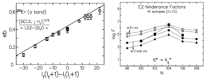
Figure 1: (Left) $E2$ transition amplitudes for the $\gamma$ vibrational band in ¹⁶⁶Er. The experimental data are taken from figure 4-30 in BM2. Adapted from reference [43]. (Right) Hindrance factors of $B(E2;6^{+}_{K=6}\rightarrow 4^{+})$ for decay of $K^{\pi}=6^{+}$ isomers in Hf isotopes. Calculated values are shown by circles, while the squares are the experimental data. See text for details. Adapted from reference [43].

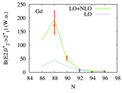
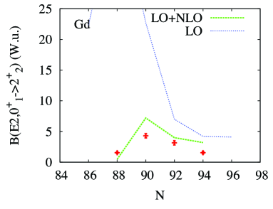
Figure 2: (Left) Calculated and experimental $B(E2;0^{+}_{\beta}\rightarrow 2^{+}_{g})$ values in Gd isotopes. Adapted from reference [37]. (Right) $B(E2;0^{+}_{g}\rightarrow 2^{+}_{\beta})$ values in Gd isotopes. Experimental data are taken from references [36, 44, 45, 46, 47, 48]. Note that the scale of the ordinate is 1/10 of that in the left panel.

A very similar figure is shown in Fig. 4-30 of BM2, however, we note here that the parameters $(Q_{t},q)$ in the left panel of figure 1 is based on the microscopic calculation, while those in BM2 are determined by fitting the experimental data. The LO relation produces the same $Q_{t}$ but $q=0$. The Coriolis coupling effect in the NLO is represented by the parameter $q$ ($m^{(\pm 1)}_{2\ \mp 1}$). For the $\gamma$ vibrations, the cranking calculation always produces $q>0$ in the rare-earth nuclei [40], which suggests the transitions $I_{\gamma}\rightarrow I_{g}$ are enhanced (hindered) for $I_{g}>I_{\gamma}$ ($I_{g}<I_{\gamma}$). This is consistent with experimental data (see reference [40] and references therein). We also obtain a reasonable agreement for the $M1$ transitions. However, the calculated sign of the $M1/E2$ mixing amplitudes changes from nucleus to nucleus, while the observed values are always negative [40].

The collectivity of the $\beta$ vibrations measured by the strengths of the interband transitions to/from the ground band is weaker than that of the $\gamma$ vibrations in most cases. However, in rare-earth nuclei in (near) the transitional region, the $\beta$ vibrations produce very low excitation energies and large $B(E2;0^{+}_{\beta}\rightarrow 2^{+}_{g})$ values. In Gd isotopes, for example, their excitation energies are 681 keV and 615 keV for ¹⁵⁴Gd ($N=90$) and ¹⁵²Gd ($N=88$), respectively. The $B(E2;0^{+}_{\beta}\rightarrow 2^{+}_{g})$ values amount to $52\pm 8$ and $178^{+53}_{-33}$ W.u. [45, 44]. We expect similar values of $B(E2;0^{+}_{g}\rightarrow 2^{+}_{\beta})$, which are predicted to be identical to $B(E2;0^{+}_{\beta}\rightarrow 2^{+}_{g})$ in the LO relation. Surprisingly, the observed $B(E2;0^{+}_{g}\rightarrow 2^{+}_{\beta})$ values are much smaller than $B(E2;0^{+}_{\beta}\rightarrow 2^{+}_{g})$ [36, 45, 44].

Figure 2 shows the calculated $B(E2)$ values using the the LO+NLO intensity relation identical to equation (29) with some trivial changes in the left hand side ($K_{i}^{\pi}=2_{\gamma}^{+}\rightarrow K_{i}^{\pi}=0_{\beta}^{+}$, $\langle I_{i}22-2|I_{f}0\rangle\rightarrow\langle I_{i}020|I_{f}0\rangle$). The LO relation cannot account at all for both large $B(E2;0^{+}_{\beta}\rightarrow 2^{+}_{g})$ and small $B(E2;0^{+}_{g}\rightarrow 2^{+}_{\beta})$ values. Owing to relatively small moments of inertia ($\mathcal{J}$) for these transitional nuclei, the inclusion of the NLO terms with large values of $q$ nicely reproduces both of them. In BM2 (pp.168–175), the band mixing between the ground and the $\beta$ bands in ¹⁷⁴Hf are presented to explain the observed intensity relations. An effect of hindrance of the shape fluctuation induced by the rotation, suggested in references [49, 50, 51], may also play an important role. The Coriolis coupling effects may be a key ingredient to understand the peculiar $B(E2)$ properties of the $\beta$-vibrational bands.

Generally speaking, the Coriolis-coupling effect for the quadrupole vibrations is relatively weak, because the low-lying $K^{\pi}=1^{+}$ collective state is missing (section 4.2). In contrast, all the members of the multiplet are present for the negative-parity octupole vibrations. Thus, we expect stronger Coriolis effects. The cranking calculation actually predict the NLO parameters of the octupole vibrations ($|q|\sim 0.1$) larger than those of $\gamma$ vibrations ($|q|\sim 0.01$) [40]. The $K$ quantum number of the lowest mode of excitation among the octupole multiplet ($K^{\pi}=0^{-}\sim 3^{-}$) changes from nucleus to nucleus. Nevertheless, the lowest mode always has $q<0$ for transitions from the octupole band ($K_{i}$) to the ground band ($K_{f}=0$), Thus, $B(E3;3^{-}\rightarrow 0^{+})$ is enhanced for the lowest mode. This Coriolis effect is clearly seen in Gd isotopes in figure 3.

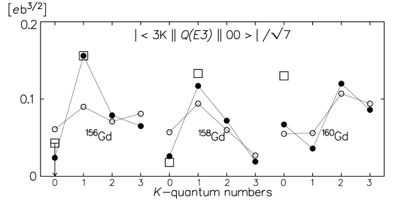
Figure 3: $E3$ transition amplitudes for the octupole vibrational states in Gd isotopes, $I_{i}^{\pi}=3^{-}\rightarrow I_{f}^{\pi}=0^{+}$. Open and filled circles correspond to calculated values in the LO and LO+NLO, respectively, compared with experimental data (open squares) [52]. The lowest mode of excitation among the octupole multiplet is $K=1$ for ^156,158Gd and $K=2$ for ¹⁶⁰Gd. From reference [53].

Another application is presented here for $K$-forbidden transitions in decays of the high-$K$ isomers. For $K$-forbidden transitions with $|\Delta K|>\lambda$, we should extend the LO+NLO relation of equation (27) because the LO term vanishes. The order of $K$ forbiddenness is defined by $n=|\Delta K|-\lambda$. The NⁿLO+Nⁿ⁺¹LO intensity relation for $\Delta K>0$ is given by [40]

$$\qquad Q^{{\rm(N}^{n}+{\rm N}^{n+1}{\rm LO)}}_{\lambda\Delta I}=m_{\lambda\ \lambda}^{(-n)}\mathcal{D}^{\lambda}_{\Delta I\lambda}(I_{-})^{n}+\frac{m_{\lambda\ \lambda-1}^{(-n-1)}}{2}\left\{(I_{-})^{n+1},{\cal D}^{\lambda}_{\Delta I\ \lambda-1}\right\}+\mathcal{R}{\rm-conj.},\quad$$ (30)

where the intrinsic moments are

$$\eqalign{m_{\lambda\ \pm\lambda}^{(\mp n)}=\frac{1}{n!\mathcal{J}^{n}}\frac{d^{n}(K_{f}|Q_{\lambda\ \pm\lambda}|K_{i})}{d\omega_{\rm rot}^{n}},\cr m_{\lambda\ \pm(\lambda-1)}^{(\mp(n+1))}=\frac{1}{(n+1)!\mathcal{J}^{n+1}}\frac{d^{n+1}(K_{f}|Q_{\lambda\ \pm(\lambda-1)}|K_{i})}{d\omega_{\rm rot}^{n+1}}.}$$ (31)

These formulae are applied to the two-quasiparticle (2qp) $K^{\pi}=6^{+}$ isomers in Hf isotopes. The configuration of the initial state $|K_{i}=6)$ is assumed to be the proton 2qp $[402\ 5/2]\otimes[404\ 7/2]$. The hindrance factors are shown in the right panel of figure 1. This is defined by

$$F\equiv\frac{B(E2;6^{+}\rightarrow 4^{+})_{W}}{B(E2;6^{+}_{K=6}\rightarrow 4^{+}_{g})},$$ (32)

where $B(E2)_{W}$ is the Weisskopf estimate of the reduced transition probability. A large hindrance factor means a long life time of the high-$K$ isomer state.

The calculated values are shown in the right panel of figure 1 by filled symbols (circles and triangles), which are compared with experiment (filled squares). The calculation qualitatively reproduces the experimental trends. However, these values turn out to be quite sensitive to the details of the quasiparticle spectra. For instance, the triangles are obtained with slightly larger values of the proton chemical potentials (by 70 keV) than those of circles. The calculated hindrance factors differ by about one order of magnitude. The effect of the residual interaction is very significant too. The open symbols in figure 1 (right) show results including the spin-spin interaction, $V_{0}\vec{\sigma}\cdot\vec{\sigma}$, with $V_{0}=100$ keV, which roughly accounts for the Gallagher-Moszkowski splitting. This could change $F$ by two order of magnitude. Nonetheless, the neutron number dependence is rather universal, that indicates the largest hindrance at $N=104$.

5.2 Cranking model at high spin: QRPA in the rotating frame

Rotating the nucleus very fast, the perturbative treatment in section 5.1 becomes no longer valid. Instead, the semiclassical treatment in the cranking model is better justifiable, and the direct application of the cranking model (19) has been extensively performed for a variety of high-spin phenomena. For instance, the famous back-bending phenomena have been studied and understood as the crossing between the ground band and an aligned 2qp band. This can be also interpreted as breaking a Cooper pair condensed in the ground band by the Coriolis anti-pairing effect.

In order to investigate properties of elementary modes of excitation at high spin, it is useful to use the “routhian” $E^{\prime}(\omega_{\rm rot})$ as a function of the rotational frequency $\omega_{\rm rot}$. The routhian here is defined as the eigenenergies of the cranking Hamiltonian (19), which can be interpreted as the energy in the rotating frame with the rotational frequency $\omega_{\rm rot}$. To make a comparison, we often convert the experimental excitation energy as a function of $I$, $E(I)$, into the “routhian” $E^{\prime}(\omega_{\rm rot})$. This is done as follows. First, from experimental rotational spectra $E_{b}(I)$, we calculate the frequency, $\omega_{\rm rot}(I)=dE_{b}(I)/dI$. Here, $b$ is the index of the rotational band. According to the cranking Hamiltonian (19), the routhian is defined as $E^{\prime}_{b}(\omega_{\rm rot})=E_{b}(I)-\omega_{\rm rot}I_{x}(I)$ with $I_{x}(I)=\sqrt{(I+1/2)^{2}-K^{2}}$, at discrete values of $\omega_{\rm rot}(I)$. The reference routhian $E^{\prime}_{\rm ref}(\omega_{\rm rot})$ is defined, for instance, by fitting that of the ground-state band (“b”=“g.s.”). Then, the excitation routhian relative to the reference band as a function of $\omega_{\rm rot}$ is obtained as $E^{\prime}_{\rm ex}(\omega_{\rm rot})=E^{\prime}_{b}(\omega_{\rm rot})-E^{\prime}_{\rm ref}(\omega_{\rm rot})$ for each band “$b$”. In Ref. [54], the experimental routhians in odd nuclei, which were obtained by adopting the reference band fitting the ground-state band in neighboring even-even nuclei, show nice agreement with the calculated quasiparticle routhians.

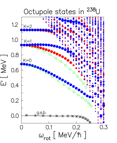
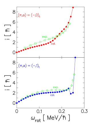
Figure 4: (Left) Excitation routhian plot as functions of rotational frequency $\omega_{\rm rot}$ for negative-parity states in ²³⁸U. Large, medium, and small circles indicate the QRPA solutions with $E3$ transition amplitudes larger than 300 $e$fm³, larger than 150 $e$fm³, and less than 150 $e$fm³, respectively. The red (blue) ones correspond to the signature even (odd) states with even (odd) $I$. Experimental routhians are plotted by open squares. (Right) Aligned angular momentum as a function of $\omega_{\rm rot}$ for the lowest ($K^{\pi}=0^{-}$) and the second lowest ($K^{\pi}=1^{-}$) octupole bands in the lower and upper panels, respectively. Open squares indicate experimental data [55]. Adapted from reference [56].

The routhian plot for the octupole vibrational bands in ²³⁸U are presented in figure 4. See references [10, 56] for details of the calculation. In the right panels, the alignment, defined by $i\equiv-dE^{\prime}/d\omega_{\rm rot}$, is shown. The alignment indicates the aligned component of the angular momentum carried by the vibrational excitation. For the lowest octupole band with $K^{\pi}=0^{-}$, the alignment quickly increases up to $i\sim 3$, which suggests that the angular momentum of the octupole phonon is almost fully aligned along the rotational axis. Then, at high spin around $\omega=0.25$ MeV, it suddenly jumps up, which suggests the breakdown of the collective vibration by a strong Coriolis force. At $\omega_{\rm rot}\gtrsim 0.25$ MeV, it becomes an aligned 2qp state. This is seen in the left panel too. The octupole collectivity (size of the circles) suddenly decreases around $\omega_{\rm rot}=0.25$ MeV. In contrast to the lowest band, the second lowest $K^{\pi}=1^{-}$ band with even $I$ shows a gradual increase in the alignment, which may suggest the gradual change of the octupole phonon into the aligned 2qp structure. The present calculation nicely agrees with the experimental data.

The argument here suggests that the vibrational excitations based on the yrast (ground-state) band tend to lose their collective character at high spin, due to the intrusion of the aligned 2qp states at low energy. In this respect, the nucleus with larger deformation may be better suited for the observation of the rapidly rotating vibrational bands. This is because the large deformation tends to hinder the alignment of the quasiparticles. Next, let us discuss such a case, the high-spin superdeformed (SD) bands.

6 Elementary excitations in superdeformed rotational bands

The SD state is characterized by a large prolate deformation of approximate two-to-one axis ratio. The shell structure at the SD shape is very different from that near the spherical shape. Since the low-lying modes of excitation strongly depend on the underlying shell structure, we may expect some new features in their properties.

6.1 Octupole vibrations with $K^{\pi}=0^{-}$ and $2^{-}$

One of the most striking features in the SD shell structure is that the single-particle levels with opposite parity ($\pi=\pm$) coexist in a single shell. Adopting a simple harmonic oscillator potential, one can easily understand this fact: Namely, for $\omega_{x}=\omega_{y}=2\omega_{z}$, an orbital with the oscillator quanta $(n_{x},n_{y},n_{z})$ is degenerate in energy with those of $(n_{x}\mp 1,n_{y},n_{z}\pm 2)$ and $(n_{x},n_{y}\mp 1,n_{z}\pm 2)$. Since the parity is determined by the total quanta $N=n_{x}+n_{y}+n_{z}$, they have different parity. Another feature is that the observed SD bands are located around the closed shell configurations corresponding to the SD magic numbers (See figure 6-50 in BM2). In contrast, the normally deformed nucleus is a consequence of the SBS and has an open-shell configuration away from the spherical magic numbers. From these simple analysis, we may expect that the collective negative-parity modes of excitation appear at low energy.

The QRPA based on the cranked Nilsson-BCS model is applied to SD bands in the $A=190$ region. The calculation predicts that the $K^{\pi}=2^{-}$ octupole states are particularly low in energy, around $E^{\prime}_{x}\lesssim 1$ MeV. Especially, in ¹⁹⁴Hg and ¹⁹⁶Pb with $N=114$, very collective $K^{\pi}=2^{-}$ octupole vibrations appear well below 1 MeV and their excitation routhians are roughly constant with very little signature splitting [10]. See the right panel of figure 5. Later, the interband $E1$ transitions between the octupole and ground SD bands have been measured for ¹⁹⁴Hg [57] and for ¹⁹⁶Pb [58], which confirms nice agreement with calculated routhians and the strong octupole collectivity. For $N=110$, the calculation predicts an aligned octupole phonon, shown in the left panel of figure 5, similar to the lowest octupole band in ²³⁸U in figure 4. This also nicely reproduces the experimental routhians in an excited SD band in ¹⁹⁰Hg [59]. Later, the linear polarization measurement confirms the aligned octupole vibrations [60].

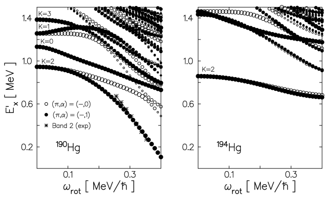
Figure 5: Excitation routhian plot for negative-parity excitations in SD ¹⁹⁰Hg (left) and ¹⁹⁴Hg (right). Open and filled circles correspond to the states with even and odd signatures, respectively. The size of circles represent the $E3$ transition amplitudes ($>200$ $e$fm³, $>100$ $e$fm³, and $<100$ $e$fm³) Experimental excitation routhians in ¹⁹⁰Hg are shown by stars ($*$). From reference [56].

In the $A=150$ region, we theoretically predicted a possible candidate of $K^{\pi}=0^{-}$ octupole band in SD ¹⁵²Dy [61]. It shows a rather constant excitation routhians in a wide range of $\omega_{\rm rot}=0\sim 0.7$ MeV. Later in 2002, its octupole character has been confirmed by the measurement of the interband transitions and the spin identification [62, 63]. The $\omega_{\rm rot}$-dependence of the routhian well agrees with the theoretical prediction.

6.2 Soft mode with $K^{\pi}=1^{-}$

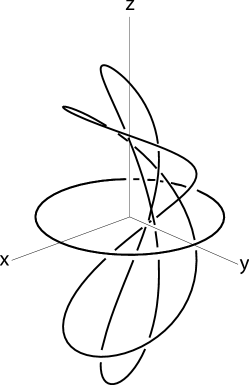
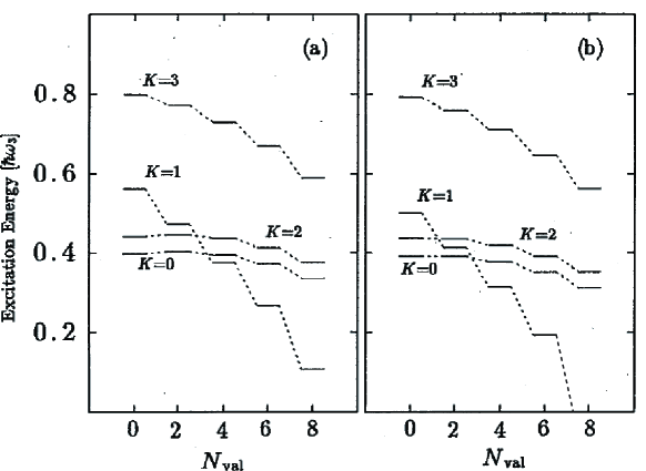
Figure 6: (Left) Typical classical periodic orbits in a potential with the $a:b:c=2:2:1$ shell structure. From reference [64]. (Right) Calculated excitation energies for octupole vibrations in the SD harmonic oscillator potential, with stronger pairing (a) and weak pairing interactions (b). From reference [65].

So far, the octupole vibrational excitations in SD rotational bands have been observed (confirmed) only for the $K^{\pi}=0^{-}$ and $2^{-}$ modes. Theoretically, these modes are predicted to appear lower than other modes ($K^{\pi}=1^{-}$ and $3^{-}$), near the SD magic numbers. However, moving away from the magic closed configurations, the $K^{\pi}=1^{-}$ modes become a soft mode.

In order to investigate the soft mode in the SD shape, we again follow the discussion in BM2 (pp. 591$-$598), extending the argument for spherical potentials in section 3.3 to a deformed one. This is possible if the motion is separable in the three coordinates, such as the harmonic oscillator potential. In a deformed harmonic oscillator potential, the single-particle energy is specified by there numbers of the oscillator quanta, $(n_{x},n_{y},n_{z})$. Thus, the shell structure is characterized by the ratio of three integers, $a:b:c$, and the shell frequency given by

$$\qquad\omega_{\rm sh}\equiv\frac{1}{a}\left(\frac{\partial\epsilon}{\partial n_{x}}\right)_{0}=\frac{1}{b}\left(\frac{\partial\epsilon}{\partial n_{y}}\right)_{0}=\frac{1}{c}\left(\frac{\partial\epsilon}{\partial n_{z}}\right)_{0}.$$ (33)

Since $a:b:c=1:1:1$ correspond to the spherical harmonic oscillator, the simplest integer ratio next to $1:1:1$ is $a:b:c=1:1:2$ and $2:2:1$. The SD shape we are discussing here corresponds to the latter one, which has the prolate shape.

The frequency ratio of $a:b:c=2:2:1$ ($\omega_{x}=\omega_{y}=2\omega_{z}=2\omega_{\rm sh}$) creates periodic orbits shown in the left panel of figure 6. These are orbits of “bending figure of eight”. Since the shape of the classical periodic orbits is related to the soft mode, the SD state, with many nucleons outside the closed shell, may be unstable against the banana-shaped bending mode.

In figure 6, we show the result of the QRPA calculation with the separable octupole interaction, based on the SD harmonic oscillator potential [65]. The $K^{\pi}=0^{-}$ and $2^{-}$ modes are the lowest near the SD magic numbers. These modes are rather insensitive to the number of nucleons outside the closed shell. However, the $K^{\pi}=1^{-}$ octupole mode dramatically decreases its energy as increasing the number of valence nucleons. With enough number of valence nucleons, the bending $K^{\pi}=1^{-}$ mode leads to the instability.

According to the qualitative discussion on the SD shell structure, Bohr and Mottelson have already pointed out the possibility of this instability toward the bending shape, in the context of fission path (p.598 in BM2). As far as we know, this effect on the fission dynamics has not been fully studied so far.

7 Nuclear wobbling motion and precession

Most of the existing experimental data are known to be consistent with the interpretation based on the axially symmetric deformation. Even the octupole deformation (section 3.3) observed in heavy nuclei is associated with the axially symmetric one ($Y_{30}$). In section 6.2, we have presented a possible exotic nuclear shape in SD nuclei away from the closed shell configuration, that breaks both the axial and the parity symmetry. However, it has not been observed in experiments.

Bohr and Mottelson gave extensive discussion on the spectra of triaxial nuclei in BM2. In the beginning of section 4-5, they said “Although, at present (1975), there are no well-established examples of nuclear spectra corresponding to asymmetric equilibrium shapes, it appears likely that such spectra will be encountered in the exploration of nuclei under new conditions (large deformations, angular momentum, isospin, etc.).” They were absolutely right.

The identification of the static triaxial deformation has been a longstanding issue in the nuclear structure physics. One of the difficulties is to confirm its “static” nature clearly distinguished from the “dynamic” one. The observation of a wobbling band was a breakthrough that provided a clear indication of the non-uniform three-dimensional rotation of a triaxial nucleus. We have really encountered this new phenomenon at large deformation and angular momentum.

The first observation of the wobbling band was in ¹⁶³Lu [66, 67]. At high spin ($I\gtrsim 20$), several regular rotational bands with large moments of inertia come down to the yrast region. The deformation of these bands have been speculated to be large ($\epsilon\sim 0.4$) and triaxial ($\gamma\sim 20^{\circ}$), according to calculations of the total routhian surface (TRS) with the Nilsson potential [68]. They are called the triaxial superdeformed (TSD) bands and labeled as TSD1, TSD2, etc. In addition to the stretched intraband transitions ($\Delta I=2$), the linking transitions ($\Delta I=1$) between TSD2 and TSD1 (yrast), between TSD3 and TSD2, and between TSD3 and TSD1, have been observed. The $E2$ character of these interband transitions is experimentally confirmed [68] and their large strengths nicely correspond to the estimate by a simple triaxial rotor model. The measured $B(E2)$ values for the interband transitions are order of 100 W.u. which is considerably larger than those of the most collective $\gamma$ vibrations.

7.1 Rotor model analysis of the wobbling in the high-spin limit

The prediction based on the rotor model given by Bohr and Mottelson (section 4-5e in BM2) is recapitulated here. The rotor Hamiltonian contains three different moments of inertia, $\mathcal{J}_{x}>\mathcal{J}_{y}>\mathcal{J}_{z}$, with respect to the principal axes in the body-fixed frame.

$$\qquad H_{\rm rot}=\frac{J_{x}^{2}}{2\mathcal{J}_{x}}+\frac{J_{y}^{2}}{2\mathcal{J}_{y}}+\frac{J_{z}^{2}}{2\mathcal{J}_{z}}=\frac{\vec{J}^{2}}{2\mathcal{J}_{x}}+\left(\frac{1}{2\mathcal{J}_{y}}-\frac{1}{2\mathcal{J}_{x}}\right)J_{y}^{2}+\left(\frac{1}{2\mathcal{J}_{z}}-\frac{1}{2\mathcal{J}_{x}}\right)J_{z}^{2}.$$ (34)

For the lowest energy (yrast) state at a given $I$, the term proportional to $\vec{J}^{2}$ in this Hamiltonian is dominant at high spin ($I\rightarrow\infty$). This corresponds to a uniform rotation around the $x$ axis: $E_{I}\approx I(I+1)/(2\mathcal{J}_{x})$. In this high-spin limit, we assume $J_{x}\approx I$ which can be treated as a $c$-number. The remaining terms of the Hamiltonian (34) can be diagonalized, $[H_{\rm rot},X_{\rm wob}^{\dagger}]=\omega_{\rm wob}X_{\rm wob}^{\dagger}$, by a linear transformation. The normal-mode (wobbling phonon) creation operator

$$X_{\rm wob}^{\dagger}\equiv a\frac{iJ_{y}}{\sqrt{2I}}-b\frac{J_{z}}{\sqrt{2I}},$$ (35)

with the normalization $\left[X_{\rm wob},X_{\rm wob}^{\dagger}\right]=1$ leads to the following relations:

$$\frac{a}{b} = \sqrt{\left(\frac{1}{\mathcal{J}_{y}}-\frac{1}{\mathcal{J}_{x}}\right)\left(\frac{1}{\mathcal{J}_{z}}-\frac{1}{\mathcal{J}_{x}}\right)^{-1}},\quad\quad ab=1,$$ (36)

$$\omega_{\rm wob} = I\sqrt{\left(\frac{1}{\mathcal{J}_{y}}-\frac{1}{\mathcal{J}_{x}}\right)\left(\frac{1}{\mathcal{J}_{z}}-\frac{1}{\mathcal{J}_{x}}\right)}.$$ (37)

The operator for the wobbling phonon number is given by $n\equiv X_{\rm wob}^{\dagger}X_{\rm wob}$. In this way, the rotor Hamiltonian can be written as a sum of the rotation around the $x$ axis and the wobbling phonon excitation: $E_{In}\approx I(I+1)/(2\mathcal{J}_{x})+\omega_{\rm wob}(n+1/2)$. A schematic figure for these spectra is shown in figure 7. In order to realize this kind of multiple band structure from one intrinsic configuration, the nucleus should be able to rotate about all three principal axes. Therefore, the nuclear shape must be triaxial. In addition, among the three moments of inertia, the one along the major rotational axis $\mathcal{J}_{x}$ must be the largest.

       

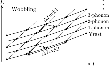
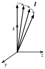
Figure 7: A schematic illustration of the wobbling motion. (Left) Excitation spectra with $\Delta I=2$ and $\Delta I=1$ sequences. (Right) A wobbling phonon excitation tilts the direction of the angular momentum from the $x$-axis. From reference [69].

According to the LO high-spin formula (20), the intraband $B(E2;\Delta I=2)$ strengths are proportional to the quadrupole deformation $(\tilde{Q}_{22})^{2}$. The $\Delta I=1$ transitions, which are associated with the wobbling transitions, appear in the NLO with respect to $1/I$; $B(E2;\Delta I=1)/B(E2;\Delta I=2)\sim 1/I$. These $E2$ transition strengths were explicitly given in chapter 4-5e in BM2. The TRS calculation predicts the “positive” $\gamma$ shape ($\gamma\sim 20^{\circ}$) for the TSD bands in ¹⁶³Lu. Here we use the so-called Lund convention for the triaxiality parameter $\gamma$ in relation to the main rotation axis [70], where for the positive $\gamma$ shape, $0<\gamma<60^{\circ}$, the rotation ($x$) axis is the shortest principal axis, while for the negative $\gamma$ shape, $-60^{\circ}<\gamma<0$, it is the intermediate principal axis. Then the out-of-band $E2$ transitions for the positive $\gamma$ shape satisfy a relation, $B(E2;I\rightarrow I-1)>B(E2;I\rightarrow I+1)$. This is consistent with the experiments, in which only the $I\rightarrow I-1$ transitions have been observed.

The simple rotor model picture, however, disagrees with the observed data with respect to the following points:

• At $\gamma=20^{\circ}$ which is supported by the TRS calculation, the $\gamma$-dependence of the irrotational moments of inertia, which are commonly assumed in the rotor model, produce $\mathcal{J}_{y}>\mathcal{J}_{x}>\mathcal{J}_{z}$. This contradicts the basic assumption of $\mathcal{J}_{x}>\mathcal{J}_{y}>\mathcal{J}_{z}$ and the formula (37).

• According to equation (37), the wobbling frequency $\omega_{\rm wob}$ increases as a function of $I$. Conversely, the observed frequency decreases.

Solutions to these problems will be provided by microscopic treatments in section 7.2.

7.2 Microscopic QRPA analysis for the wobbling motion

A microscopic theory to treat the nuclear wobbling motion in the small amplitude limit is naturally provided by the QRPA in the rotating frame, or the self-consistent cranking plus QRPA [71]. Among the quadrupole tensors, $Q_{ij}\propto x_{i}x_{j}-\delta_{ij}r^{2}/3$ ($i,j=x,y,z$), the negative signature operators of $Q_{y}\equiv-Q_{zx}$ and $Q_{z}=iQ_{xy}$ are responsible for the wobbling motion. Adopting the separable quadrupole interaction of the form (7), the mean-field approximation simply replaces one of the operators $QQ$ into its expectation value $\mathcal{Q}(t)$, leading to the time-dependent mean field

$$h_{\rm UR}(t)=h_{\rm def}-\omega_{\rm rot}J_{x}-\kappa_{y}\mathcal{Q}_{y}(t)Q_{y}-\kappa_{z}\mathcal{Q}_{z}(t)Q_{z},$$ (38)

where $h_{\rm def}$ is a deformed single-particle Hamiltonian that contains the fields associated with diagonal tensors, $-\kappa_{ii}\mathcal{Q}_{ii}Q_{ii}$. Although, in general, $h_{\rm def}$ is time-dependent, we hereafter focus our discussion on the wobbling motion, and assume $h_{\rm def}$ is time-independent. In this treatment of equation (38), the rotational axis stays along the $x$ axis and the wobbling motion is represented by a fluctuation in the orientation of deformed density distribution induced by $\mathcal{Q}_{y}(t)$ and $\mathcal{Q}_{z}(t)$. This picture corresponds to the uniformly rotating (UR) frame.

The small shape fluctuation induced by the off-diagonal quadrupole tensors, $\mathcal{Q}_{y}$ and $\mathcal{Q}_{z}$, is not associated with the real shape change from the equilibrium. The same effect can be realized by rotating the reference frame to the principal axis (PA) frame where the non-diagonal elements, $Q_{y}$ and $Q_{z}$, of the quadrupole tensors vanish. If we adopt this body-fixed frame, the direction of the angular momentum fluctuates. In the PA frame, since the rotation is no longer uniform, the cranking model should be extended to a time-dependent one.

$$h_{\rm PA}(t)=h_{\rm def}-\vec{\omega}_{\rm rot}(t)\cdot\vec{J}.$$ (39)

The rotor-model analysis of Bohr and Mottelson in section 7.1 has a direct connection to the PA picture. In this picture, the frequency $\vec{\omega}_{\rm rot}$ should be treated as dynamical variables (operators). In the small amplitude limit, Marshalek proved the equivalence between the UR and the PA frames and obtained the same expression (37) for the wobbling frequency, with the moments of inertia calculated in the QRPA [71]. It is generalized to arbitrary mean-field potentials and residual interactions [11]. The two pictures are schematically illustrated in figure 8.

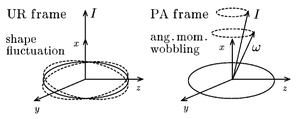
Figure 8: Two equivalent pictures of the wobbling motion: one in the uniformly rotating (UR) frame (left) and the other in the principal axis (PA) frame (right). From reference [69].

The microscopic QRPA calculations were first performed with the Nilsson potential and the separable quadrupole interactions [72, 73, 74, 75, 76]. Later, it has been done with the Woods-Saxon potential and an separable interaction which is determined by the symmetry restoration condition [11]. In general, it is difficult to perform the QRPA calculation for an odd-$A$ nucleus, however, this is not a problem at a finite $\omega_{\rm rot}$ because the Kramers degeneracy is lifted and the RPA vacuum is uniquely identified. The calculated QRPA moments of inertia indicate a proper ordering of moments of inertia, $\mathcal{J}_{x}>\mathcal{J}_{y}>\mathcal{J}_{z}$, for the wobbling mode in ¹⁶³Lu. Why is this ordering different from a naive expectation based on the irrotational flow?

To answer the question, it is important to distinguish the dynamic and the kinematic moments of inertia [77]. The dynamic moment of inertia is defined by the second derivative of the rotational energy, $1/\mathcal{J}^{(2)}=d^{2}E_{I}/dI^{2}$, which is considered to be the one in the rotor model in equation (34). In contrast, the kinematic moment of inertia is defined by the first derivative, $1/\mathcal{J}^{(1)}=I^{-1}dE_{I}/dI=\omega_{\rm rot}/I$. The largest moment of inertia, $\mathcal{J}_{x}$, in the QRPA wobbling formalism of reference [71] is the kinematic one, more precisely, $\mathcal{J}_{x}=\mathcal{J}^{(1)}_{x}\equiv\langle J_{x}\rangle/\omega_{\rm rot}$, which is strongly influenced by the alignment of the intrinsic angular momentum along the rotational ($x$) axis. Generally the kinematic moment of inertia is larger than the dynamic one because of the effect of alignment. In ¹⁶³Lu, the odd-proton quasiparticle mainly produces the alignment. When the alignment is large enough, we could have a rigid-body-like ordering, $\mathcal{J}_{x}^{(1)}>\mathcal{J}_{y}>\mathcal{J}_{z}$, for the positive $\gamma$ shape, even if the dynamic moments of inertia are irrotational-like, $\mathcal{J}_{y}>\mathcal{J}_{x}>\mathcal{J}_{z}$. The QRPA moments of inertia automatically take into account this effect. Thus, the alignment effect is crucial for the appearance of the wobbling mode, which was first pointed out in references [74, 75].

The fact that the largest moment of inertia is the kinematic one can be justified by the simple particle-rotor model as in reference [78]: When the quasiparticle alignment $j$ is present, $J_{x}$ is replaced by $J_{x}-j$ in equation (34). Using $J_{x}=[{\vec{J}^{2}-(J_{y}^{2}+J_{z}^{2})}]^{1/2}\approx(I+\frac{1}{2})-(J_{y}^{2}+J_{z}^{2})/(2I+1)$ which is valid for in high-spin limit $I\gg 1$, we obtain

$$H_{\scriptsize\mbox{p-rot}}=\frac{(J_{x}-j)^{2}}{2\mathcal{J}_{x}}+\frac{J_{y}^{2}}{2\mathcal{J}_{y}}+\frac{J_{z}^{2}}{2\mathcal{J}_{z}}\approx\frac{(I-j)(I-j+1)}{2\mathcal{J}_{x}}$$ (40)

$$+\left(\frac{1}{2\mathcal{J}_{y}}-\frac{1}{2\mathcal{J}_{x}}+\frac{1}{2\mathcal{J}_{x}}\frac{j}{I+\frac{1}{2}}\right)J_{y}^{2}+\left(\frac{1}{2\mathcal{J}_{z}}-\frac{1}{2\mathcal{J}_{x}}+\frac{1}{2\mathcal{J}_{x}}\frac{j}{I+\frac{1}{2}}\right)J_{z}^{2}.$$ (41)

Namely the inverse of the kinematic moment of inertia,

$$\frac{1}{\mathcal{J}_{x}^{(1)}}=\frac{\omega_{\rm rot}}{\langle J_{x}\rangle}\approx\frac{1}{\mathcal{J}_{x}}\left(1-\frac{j}{I+\frac{1}{2}}\right),$$ (42)

appears in equation (41) in place of $1/\mathcal{J}_{x}$ in equation (34).

The wobbling frequency (37) with $1/\mathcal{J}_{x}$ replaced by $1/\mathcal{J}_{x}^{(1)}$ of equation (42) first increases as spin increases and then turns to decrease. Thus the quasiparticle alignment also explains why the observed wobbling frequency decreases as a function of $I$. From equations (41) there is a critical angular momentum, $I_{c}\equiv j(1-\mathcal{J}_{x}/\mathcal{J}_{y})^{-1}-\frac{1}{2}$, at which the wobbling frequency vanishes, $\omega_{\rm wob}=0$ (remember $\mathcal{J}_{y}>\mathcal{J}_{x}>\mathcal{J}_{z}$). Beyond $I_{c}$, the wobbling mode ceases to exist, because of the irrotational-like ordering, $\mathcal{J}_{y}>\left.\mathcal{J}_{x}^{(1)}\right|_{I>I_{c}}>\mathcal{J}_{z}$. In this way, for the case where the alignment takes place along the axis of the intermediate dynamic moment of inertia, the $I$-dependence of the original wobbling frequency in section 7.1 drastically changes. Such a novel wobbling scheme was first pointed out in reference [79], although the terms proportional to $j$ in equation (41), i.e. the effect of alignment, are interpreted as decreasing $\mathcal{J}_{y}$ and $\mathcal{J}_{z}$ instead of increasing $\mathcal{J}_{x}$. The observed decreasing tendency of $\omega_{\rm wob}$ in the Lu isotopes clearly suggests such a character. In reference [78] it is called “transverse wobbler” in order to distinguish it from “longitudinal wobbler” where the quasiparticle aligns along the axis of the largest inertia, $\mathcal{J}_{x}>\mathcal{J}_{y}>\mathcal{J}_{z}$. In the longitudinal wobbler, the frequency $\omega_{\rm wob}$ monotonically increases with $I$. In fact, the microscopic QRPA calculations also predicted the wobbling motion of increasing $\omega_{\rm wob}$ as a function of $I$ in nuclei of negative $\gamma$ shapes [72, 73], in which the irrotational-type moments of inertia satisfy the longitudinal condition, $\mathcal{J}_{x}>\mathcal{J}_{y}>\mathcal{J}_{z}$. A similar argument of the effect of alignment for the possible decrease of $\omega_{\rm wob}$ has been discussed also in reference [80].

It should be noticed that the three moments of inertia are assumed to be independent of spin $I$ in the rotor model or the particle-rotor model. In reality, however, the microscopically calculated QRPA moments of inertia change as functions of $I$, although their dependencies on $I$ are not so strong in most cases [72, 73, 74, 75, 11]. One should take this into account in order to study precisely how the wobbling frequency changes as a function of spin. In reference [81], introducing a rather strong spin-dependence common to all three moments of inertia, the decreasing tendency of $\omega_{\rm wob}$ is realized in the particle-rotor coupling model with the inertia of the rigid-body-like ordering, $\mathcal{J}_{x}>\mathcal{J}_{y}>\mathcal{J}_{z}$.

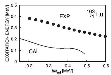
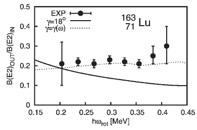
Figure 9: (Left) Calculated and experimental wobbling frequencies as functions of the rotational frequency. (Right) Calculated and experimental inter- to intraband $B(E2)$ ratio as functions of the rotational frequency. See text for details. Adapted from reference [11].

In figure 9, we show results of the QRPA calculation based on the deformed Woods-Saxon potential [11]. Note that there are no adjustable parameters in the calculation because the minimal symmetry restoring interaction is employed, which is uniquely fixed once the deformed mean-field is given. The deformation parameters are determined by minimizing the TRS. The calculated wobbling frequency has a proper trend, though the absolute magnitude is underestimated by a few hundred keV. The large interband $B(E2)$ values are rather well reproduced in the calculation. However, the observed ratio, $B(E2;I\rightarrow I-1)_{\rm out}/B(E2;I\rightarrow I-2)_{\rm in}$, seems to increase as a function of $I$, while the calculated ratio decreases because of the $1/I$ dependence of the interband transition. The dotted line in the right panel of figure 9 indicates the result obtained by artificially increasing the triaxiality ($\gamma$) at higher spins. In fact, in order to explain the experimental $B(E2)$ ratios, the triaxial parameters $\gamma({\rm den})\approx 20^{\circ}$ are necessary. The $\gamma({\rm den})$ is defined with respect to the intrinsic quadrupole moments calculated from the density distribution. Here, it should be noted that the triaxial parameter $\gamma$ for the potential shape is significantly different from $\gamma({\rm den})$ [76] (See A for details). As far as we know, at present, none of the microscopic calculations are able to reproduce the triaxiality of $\gamma({\rm den})\approx 20^{\circ}$. Another unsolved problem is that the observed $B(M1)$ values are significantly overestimated. In reference [82], the inclusion of the isovector separable orbital angular momentum interaction is suggested to improve the agreement. The nuclear wobbling motion has not been fully understood yet.

7.3 Precession: Rotational band built on a high-$K$ isomer

In section 7.2, we show that the alignment of quasiparticle is crucial for the wobbling motion to appear in the Lu isotopes with the positive $\gamma$ shape. An interesting extreme case of the alignments is that the nuclear shape is axially symmetric about the alignment ($x$) axis; i.e. $\gamma=60^{\circ}$ (oblate) or $\gamma=-120^{\circ}$ (prolate) in the Lund convention and the angular momentum is supplied only by the alignments of quasiparticles. It is expected that the optimal configurations of aligned quasiparticles in the states of such shapes make the high-spin isomers, or the “yrast traps”, along the yrast line, see e.g. reference [83]. Although the rotational bands built on the oblate isomers are not yet observed, those on the prolate isomers have been well known [1]. They are nothing but the high-$K$ rotational bands widely observed in the Hf and W region, where many high-$j$ and high-$\Omega$ Nilsson orbits are concentrated near the Fermi surface. Here, $\Omega$ is the component of single-particle angular momentum along the symmetry axis.

       

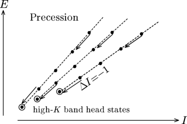
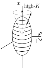
Figure 10: A schematic illustration of the precession motions. (Left) Excitation spectra from reference [84]. There are no ${\Delta I}=2$ horizontal sequences leaving only one ${\Delta I}=1$ vertical band for each high-$K$ state; compare with figure 7. (Right) Superposition of the collective rotation about the perpendicular axis makes the high-$K$ aligned angular momentum vector to precess around the symmetry axis.

We call this rotational motion “precession” because the aligned angular momentum vector tilts like in the case of the wobbling motion by superimposing the collective rotation about the perpendicular axis; it is illustrated schematically in figure 10. Since the high-$K$ isomers have been known for many years, they have been investigated by various methods; e.g., by the cranked mean-field method [85], by the RPA method based on the sloping Fermi surface [86, 87, 88, 89], or by the tiled axis cranking method [90]. In reference [84] it was considered as the axially symmetric limit of the RPA wobbling formalism [71] discussed in section 7.2. In fact, the wobbling frequency in equation (37) becomes $\omega_{\rm wob}=I/{\cal J}_{\bot}-\omega_{\rm rot}$, where the perpendicular moment of inertia is denoted as ${\cal J}_{\bot}\equiv{\cal J}_{y}={\cal J}_{z}$ in the axially symmetric limit and the rotational frequency about the main rotation axis is $\omega_{\rm rot}=I/{\cal J}^{(1)}_{x}$. Here, the dynamic moment of inertia (${\cal J}_{x}\rightarrow 0$) is replaced by the kinematic inertia ${\cal J}^{(1)}_{x}$ with the aligned angular momentum $I_{x}=K$ (we here use $K$ in place of $j$). On the other hand the rotor Hamiltonian (34) in this case reduces to $H_{\rm rot}=(I_{y}^{2}+I_{z}^{2})/(2{\cal J}_{\bot})$ so that the energy spectrum is given simply by $E_{{\scriptsize\mbox{high-}}K}=[I(I+1)-K^{2}]/(2{\cal J}_{\bot})$, which can be rewritten as

$$E_{{\scriptsize\mbox{high-}}K}=\omega_{\rm prec}\Bigl{(}n+\frac{1}{2}+\frac{n(n+1)}{2K}\Bigr{)},$$ (43)

introducing the precession phonon number $n\equiv I-K$. Here the precession frequency is given by $\omega_{\rm prec}\equiv K/{\cal J}_{\bot}=[\omega_{\rm wob}+\omega_{\rm rot}]_{I=K}$. Thus the precession motion can be described by the harmonic excitation of $n$-phonons as long as $n\ll K$. The difference of frequencies $\omega_{\rm prec}$ from $\omega_{\rm wob}$ is due to the fact that the wobbling motion is treated in the body-fixed frame while the precession motion in the laboratory-frame. Remember the transformation of the energy into the routhian in the rotating frame in section 5.2, $E^{\prime}=E-\omega_{\rm rot}I_{x}$, and that the precession mode transfer the angular momentum by one unit $\Delta I_{x}=1$. Since there is no collective rotation about $x$ axis, the rotational frequency $\omega_{\rm rot}$ is a redundant variable and any observable quantities do not depend on it; $\omega_{\rm wob}$ does depend while $\omega_{\rm prec}$ does not. As it is discussed in reference [84] not only the energy but also the electromagnetic transitions, like $E2$ and $M1$, can be treated with the multi-phonon picture as long as the phonon number $n$ is much smaller than $K$.

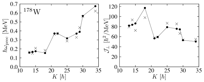
Figure 11: (Left) Calculated (filled circles) and experimental (crosses) precession frequencies $\omega_{\rm prec}$ for various high-$K$ isomers in ¹⁷⁸W, where the experimental data is denoted by crosses. (Right) Calculated (filled circles) and experimental (crosses) moments of inertia perpendicular to the symmetry axis, estimated by ${\cal J}_{\bot}=K/\omega_{\rm prec}$. Based on the result of reference [91].

We show in figure 11 the result of precession frequencies for a number of $K$ isomers in ¹⁷⁸W calculated by using the axially symmetric limit of the Woods-Saxon QRPA wobbling formalism [11]. Compared with the corresponding calculation of reference [84], in which the Nilsson mean-field potential is employed, considerable improvement can be seen and a good agreement with experimental data is obtained. In the right panel of figure 11, the estimated moments of inertia ${\cal J}_{\bot}=K/\omega_{\rm prec}$ are also shown. The agreement is much better than the simple mean-field calculation, e.g. [85], because the effect of residual interaction is taken into account in the QRPA. It can be seen that the moments of inertia take various values depending on the isomer configurations. They are considerably larger than the moment of inertia of the ground state rotational band estimated from the first $2^{+}$ state, $\mathcal{J}_{\rm gr}\approx 28$ [$\hbar^{2}$/MeV]. They do not show a simple correlation with the $K$ quantum number, and do not approach to the rigid-body value (with $\epsilon_{2}=0.240$). ${\cal J}_{\rm rig}\approx 88$ [$\hbar^{2}$/MeV], even at considerably high spin. Their properties strongly depend on what kind of quasiparticles contribute to those high-$K$ isomers in which the numbers of quasiparticles are from four to ten. See reference [84] for precise configuration assignments. At an extreme high spin, we can even imagine possible existence of torus-shape isomers and their precession motions [92].

8 Summary

Bohr and Mottelson have explored a variety of fields in the nuclear structure physics. Among them, we have discussed selected topics related to the nuclear deformation and rotation. First, we presented the concept of the symmetry breaking in the unified model. The symmetry broken state is not stable in finite systems, such as nuclei. The correlation time induced by the quantum fluctuation is a key to understand the interplay between the symmetry breaking and restoration. The finite-size effect associated with the zero-point motion may hinder the symmetry breaking.

The coupling between intrinsic and rotational motions is well described by the cranking model. Since the model assumes a semiclassical treatment of the nuclear rotation (angular momentum), the model requires the quantization in the low-spin limit. We show a possible quantization of the cranking model, which is applicable to calculation of transition matrix elements at low spin. This can be regarded as a kind of hybrid model of the unified model and the cranking model. It is applied to electromagnetic decay properties of vibrational bands and high-$K$ isomers.

In the high-spin region, the cranking model is a golden tool to study the nuclear structure under a strong Coriolis and centrifugal field. We discussed effects of the rapid rotation on the octupole vibrations, which are nicely treated with the QRPA in the uniformly rotating frame (one-dimensional cranking). The calculation reproduces the experimental data, showing the phonon alignment and loss of collectivity (phonon breakdown).

The closed shell configurations of the superdeformed (SD) states are characterized by the $2:2:1$ shell structure. This shell structure has the $K^{\pi}=1^{-}$ octupole mode as a soft mode. Away from the SD magic numbers with many valence nucleons, the prolate SD nucleus could show instability toward a bending banana shape.

The triaxial deformation produces the three dimensional non-uniform rotation, which is called wobbling motion. The QRPA in the uniformly rotating frame provides a microscopic tool to calculate the wobbling and precession modes of excitation. The experimental data are qualitatively reproduced. This microscopic study clearly indicates the importance of the quasiparticle alignment for the existence of the wobbling mode. The self-consistently calculated triaxial deformation seems to be smaller than what experimental data indicate, which is an important open problem.

The nucleus provides a wonderful opportunity to study a finite system going through many kinds of symmetry breaking, under a variety of extreme circumstances, such as large angular momentum, deformation, and isospin. The topics we have discussed in this paper were pioneered by Bohr and Mottelson who gave us a deep insight into nuclear structure and quantum many-body physics. There are still many open issues in these fields which are waiting for future studies.

Appendix A Remarks on the triaxial deformation

The values of the triaxiality parameter $\gamma$ can be significantly different depending on their definitions. This was first pointed out in the Appendix B of reference [34] and more recently discussed again in relation to the wobbling motion in reference [76]. The most basic definition is $\gamma(\mbox{den})\equiv-\tan^{-1}(\langle Q_{22}\rangle/\langle Q_{20}\rangle)$ by using the intrinsic quadrupole moments, which is directly related to the $E2$ transition probability. In phenomenological potential models, such as the Nilsson and the Woods-Saxon potentials, the triaxial deformation $\gamma\equiv\gamma(\mbox{pot})$ is introduced to define the shape of the potential. For example, it is defined based on the stretched coordinate in the Nilsson model, $\gamma(\mbox{pot:Nils})$, and on the radius parametrization $R(\theta,\phi)\propto(1+\sum a_{\lambda\mu}Y_{\lambda\mu})$ in the Woods-Saxon model, $\gamma(\mbox{pot:WS})$.

With the uniform density assumption, the triaxiality parameter $\gamma(\mbox{geo})$ can be calculated in the same way as $\gamma(\mbox{den})$ for a given $\gamma(\mbox{pot})$. Then, $\gamma(\mbox{den})\approx\gamma(\mbox{geo})$ holds in a good approximation near the self-consistent point [76], reflecting the short-range nature of the nucleon-nucleon interaction. However, it should be noted that $\gamma(\mbox{geo})$ is different from $\gamma(\mbox{pot})$, see e.g. reference [93]. These different definitions are sometimes confused.

Here we would like to take another well-known example for the harmonic oscillator model with the quadrupole deformed potential, $-(\omega/b^{2})\beta[\cos\gamma\,Q_{20}-\sin\gamma(Q_{22}+Q_{2-2})/\sqrt{2}]$, where $b$ is the oscillator length parameter for the frequency $\omega$, and we call these $\beta$ and $\gamma$ as the (pot:HO)-parametrization. Then the deformed shape of potential is the ellipsoid with the anisotropic frequencies $\omega_{k}^{2}=\omega^{2}[1-\sqrt{\frac{5}{4\pi}}\beta\cos(\gamma+\frac{2\pi}{3}k)]$ ($k=1,2,3=x,y,z$). As is discussed in section 3.4, the isotropic velocity distribution condition in equation (14) leads to $\langle x^{2}_{k}\rangle\propto\omega_{k}^{-2}$ and then $\gamma(\mbox{den})=\gamma(\mbox{geo})=\tan^{-1}[\sqrt{3}(\omega_{y}^{-2}-\omega_{x}^{-2})/(2\omega_{z}^{-2}-\omega_{x}^{-2}-\omega_{y}^{-2})]\approx(1-3\sqrt{\frac{5}{4\pi}}\beta)\gamma$ for $\beta,|\gamma|\ll 1$, which shows that the $\gamma(\mbox{geo})$ can be very different from $\gamma\equiv\gamma(\mbox{pot:HO})$ for larger $\beta\equiv\beta(\mbox{pot:HO})$ values. Similar differences are pointed out for the Nilsson and the Woods-Saxon potentials in reference [76]. Introducing $\epsilon=\sqrt{\frac{45}{16\pi}}\beta$ in place of $\beta$, we have

$$\gamma(\mbox{geo})\approx(1-2\epsilon)\gamma(\mbox{pot:HO})\approx(1-\frac{3}{2}\epsilon)\gamma(\mbox{pot:Nils})\approx(1-\frac{8}{7}\epsilon)\gamma(\mbox{pot:WS}).$$ (44)

Strictly speaking, the $\epsilon$ is also different in each definition, but that is neglected here. The difference between $\gamma(\mbox{geo})$ and $\gamma(\mbox{pot})$ is largest for the (pot:HO)-parametrization among these three examples.

The deformed shape for the wobbling motion in the Lu isotopes is predicted to be $\epsilon\sim 0.4$ and $\gamma\sim 20^{\circ}$ [68] in the (pot:Nils)-parametrization. Assuming purely ellipsoidal shape it leads to $\gamma(\mbox{geo})\approx 11^{\circ}$ [76], which is significantly smaller than the value $20^{\circ}$. The experimentally measured $B(E2)$ values seem to indicate $\gamma(\mbox{den})\approx 20^{\circ}$ or even larger values at higher spins [11]. In order to obtain $\gamma(\mbox{geo})\approx\gamma(\mbox{den})\approx 20^{\circ}$, $\gamma(\mbox{pot:Nils})\approx 31^{\circ}$ and $\gamma(\mbox{pot:HO})\approx 36^{\circ}$ are necessary with keeping $\epsilon(\mbox{pot:Nils})\approx 0.4$. In the same way, assuming only the quadrupole deformation, $\gamma(\mbox{pot:WS})\approx 28^{\circ}$ is necessary with $\beta(\mbox{pot:WS})\approx 0.4\times\sqrt{\frac{16\pi}{45}}$. Thus the required values of the potential triaxiality parameters are considerably larger, which are not obtained in any TRS calculations. The situation is the same for the self-consistent mean-field calculation. For example, we obtain $\gamma(\mbox{den})\approx 11^{\circ}$ for ¹⁶³Lu by the cranked HFB calculation with the Gogny D1S force [94], which is consistent with the Nilsson TRS calculations. None of the microscopic calculations are able to reproduce the triaxiality of $\gamma(\mbox{den})\approx 20^{\circ}$, see also reference [82].

References

References

- [1] Bohr A and Mottelson B R 1975 Nuclear Structure, Vol. II (New York: W. A. Benjamin)
- [2] Anderson P W 1952 Phys. Rev. 86(5) 694–701
- [3] Anderson P W 1958 Phys. Rev. 110(4) 827–835
- [4] Anderson P W 1958 Phys. Rev. 112(6) 1900–1916
- [5] Nambu Y 1960 Phys. Rev. 117(3) 648–663
- [6] Nambu Y and Jona-Lasinio G 1961 Phys. Rev. 122(1) 345–358
- [7] Goldstone J 1961 Il Nuovo Cimento (1955-1965) 19 154–164
- [8] Shimizu Y R and Matsuyanagi K 1982 Prog. Theor. Phys. 67 1637–1640
- [9] Mizutori S, Shimizu Y R and Matsuyanagi K 1990 Prog. Theor. Phys. 83 666–670
- [10] Nakatsukasa T, Matsuyanagi K, Mizutori S and Shimizu Y R 1996 Phys. Rev. C 53 2213–2226
- [11] Shoji T and Shimizu Y R 2009 Prog. Theor. Phys. 121 319–355
- [12] Matsuzaki M, Shimizu Y R and Matsuyanagi K 1988 Prog. Theor. Phys. 79 836–862
- [13] Nakatsukasa T, Mizutori S and Matsuyanagi K 1993 Prog. Theor. Phys. 89 847–854
- [14] Matsuzaki M 2014 Phys. Rev. C 90(4) 044313
- [15] Villars F M 1984 Nucl. Phys. A 420 61 – 82
- [16] Jahn H A and Teller E 1937 Proc. R. Soc. London A 161 220–235
- [17] Berry M V 1984 Proc. R. Soc. London A 392 45–57
- [18] Baranger M and Kumar K 1965 Nucl. Phys. 62 113 – 132
- [19] Kumar K and Baranger M 1968 Nucl. Phys. A 110 529 – 554
- [20] Bes D and Sorensen R A 1969 The pairing-plus-quadrupole model Advances in Nuclear Physics (Adv. Phys. Part. Nucl. vol 2) ed Negele J and Vogt E (Plenum Press) p 129
- [21] Brink D and Broglia R A 2005 Nuclear Superfluidity, Pairing in Finite Systems (Cambridge: Cambridge University Press)
- [22] Ring P and Schuck P 1980 The nuclear many-body problems Texts and monographs in physics (New York: Springer-Verlag)
- [23] Yannouleas C and Landman U 2007 Rep. Prog. Phys. 70 2067
- [24] Brack M, Damgaard J, Jensen A S, Pauli H C, Strutinsky V M and Wong C Y 1972 Rev. Mod. Phys. 44 320–405
- [25] Butler P A and Nazarewicz W 1996 Rev. Mod. Phys. 68(2) 349–421
- [26] Frisk H 1990 Nucl. Phys. A 511 309 – 323
- [27] Tajima N and Suzuki N 2001 Phys. Rev. C 64(3) 037301
- [28] Hamamoto I and Mottelson B R 2009 Phys. Rev. C 79(3) 034317
- [29] Takahara S, Onishi N, Shimizu Y R and Tajima N 2011 Phys. Lett. B 702 429 – 432
- [30] Arita K i 2012 Phys. Rev. C 86(3) 034317
- [31] Lister C J, Campbell M, Chishti A A, Gelletly W, Goettig L, Moscrop R, Varley B J, James A N, Morrison T, Price H G, Simpson J, Connel K and Skeppstedt O 1987 Phys. Rev. Lett. 59(12) 1270–1273
- [32] Swiatecki W 1982 Nucl. Phys. A 376 275 – 291
- [33] Heyde K and Wood J L 2011 Rev. Mod. Phys. 83(4) 1467–1521
- [34] Shimizu Y R and Matsuyanagi K 1984 Prog. Theor. Phys. 71 960–972
- [35] Pekker D and Varma C 2015 Ann. Rev. Cond. Matt. Phys. 6 269–297
- [36] Garrett P E 2001 J. Phys. G 27 R1
- [37] Matsuzaki M and Ueno T 2016 Prog. Theor. Exp. Phys. 2016 043D03
- [38] Harakeh M N and van der Woude A 2001 Giant resonances Oxford Studies in Nuclear Physics 24 (Oxford: Oxford University Press)
- [39] Blaizot J P and Ripka G 1986 Quantum Theory of Finite Systems (Cambridge: MIT Press)
- [40] Shimizu Y R and Nakatsukasa T 1996 Nucl. Phys. A 611 22–46
- [41] Marshalek E 1976 Nucl. Phys. A 266 317 – 336
- [42] Marshalek E 1977 Nucl. Phys. A 275 416 – 444
- [43] Nakatsukasa T and Shimizu Y R 1999 J. Phys. G 25 795–797
- [44] Martin M J 2013 Nucl. Data Sheets 114 1497 – 1847
- [45] Reich C W 2009 Nucl. Data Sheets 110 2257 – 2532
- [46] Reich C W 2012 Nucl. Data Sheets 113 2537 – 2840
- [47] Helmer R G 2004 Nucl. Data Sheets 101 325 – 519
- [48] Reich C W 2005 Nucl. Data Sheets 105 557 – 774
- [49] Hinohara N, Nakatsukasa T, Matsuo M and Matsuyanagi K 2009 Phys. Rev. C 80 014305
- [50] Hinohara N, Sato K, Nakatsukasa T, Matsuo M and Matsuyanagi K 2010 Phys. Rev. C 82 064313
- [51] Hinohara N, Sato K, Yoshida K, Nakatsukasa T, Matsuo M and Matsuyanagi K 2011 Phys. Rev. C 84(6) 061302
- [52] McGowan F K and Milner W T 1981 Phys. Rev. C 23(5) 1926–1937
- [53] Nakatsukasa T and Shimizu Y R 1997 Prog. Part. Nucl. Phys. 38 247–248
- [54] Bengtsson R and Frauendorf S 1979 Nucl. Phys. A 327 139 – 171
- [55] Ward D, Andrews H, Ball G, Janzen V, Nakatsukasa T, Radford D, Galindo-Uribarri A, Drake T, deGraaf J, Pilotte S and Shimizu Y R 1996 Nucl. Phys. A 600 88–110
- [56] Nakatsukasa T 1996 Acta Phys. Pol. B 27 59–70
- [57] Hackman G, Khoo T, Carpenter M, Lauritsen T, Lopez-Martens A, Calderin I, Janssens R, Ackermann D, Ahmad I, Agarwala S, Blumenthal D, Fischer S, Nisius D, Reiter P, Young J, Amro H, Moore E, Hannachi F, Korichi A, Lee I, Macchiavelli A, Dössing T and Nakatsukasa T 1997 Phys. Rev. Lett. 79 4100–4103
- [58] Roßbach D, Görgen A, Hübel H, Mergel E, Schönwaßer G, Wilson A, Azaiez F, Astier A, Bazzacco D, Bergström M, Bourgeois C, Buforn N, Hannachi F, Hauschild K, Korichi A, Korten W, Kröll T, Lopez-Martens A, Lucas R, Maier H, Redon N, Reiter P, Rossi-Alvarez C, Stezowski O and Thirolf P 2001 Phys. Lett. B 513 9 – 14
- [59] Wilson A, Timár J, Sharpey-Schafer J, Crowell B, Carpenter M, Janssens R, Blumenthal D, Astier A, Azaiez F, Bergström M, Ducroux L, Gall B, Hannachi F, Korichi A, Lopez-Martens A, Meyer M, Paul E, Porquet M, Redon N, Wilson J and Nakatsukasa T 1996 Phys. Rev. C 54 559–567
- [60] Korichi A, Wilson A N, Hannachi F, Lopez-Martens A, Rejmund M, Schück C, Vieu C, Chmel G, Görgen A, Hübel H, Rossbach D, Schönwasser S, Bergström M, Nyakó B M, Timár J, Bazzacco D, Lunardi S, Rossi-Alvarez C, Bednarczyk P, Kintz N, Naguleswaran S, Astier A, Cullen D M, Sharpey-Schafer J F, Lauritsen T and Wadsworth R 2001 Phys. Rev. Lett. 86(13) 2746–2749
- [61] Nakatsukasa T, Matsuyanagi K, Mizutori S and Nazarewicz W 1995 Phys. Lett. B 343 19–24
- [62] Lauritsen T, Carpenter M P, Døssing T, Fallon P, Herskind B, Janssens R V F, Jenkins D G, Khoo T L, Kondev F G, Lopez-Martens A, Macchiavelli A O, Ward D, Abu Saleem K S, Ahmad I, Clark R, Cromaz M, Greene J P, Hannachi F, Heinz A M, Korichi A, Lane G, Lister C J, Reiter P, Seweryniak D, Siem S, Vondrasek R C and Wiedenhöver I 2002 Phys. Rev. Lett. 88(4) 042501
- [63] Lauritsen T, Janssens R V F, Carpenter M P, Fallon P, Herskind B, Jenkins D G, Khoo T L, Kondev F G, Lopez-Martens A, Macchiavelli A O, Ward D, Saleem K A, Ahmad I, Clark R M, Cromaz M, Døssing T, Heinz A M, Korichi A, Lane G, Lister C J and Seweryniak D 2002 Phys. Rev. Lett. 89(28) 282501
- [64] Mizutori S, Nakatsukasa T, Arita K, Shimizu Y R and Matsuyanagi K 1993 Nucl. Phys. A 557 125c–144c
- [65] Nakatsukasa T, Mizutori S and Matsuyanagi K 1992 Prog. Theor. Phys. 87 607–626
- [66] Ødegård S W, Hagemann G B, Jensen D R, Bergström M, Herskind B, Sletten G, Törmänen S, Wilson J N, Tjøm P O, Hamamoto I, Spohr K, Hübel H, Görgen A, Schönwasser G, Bracco A, Leoni S, Maj A, Petrache C M, Bednarczyk P and Curien D 2001 Phys. Rev. Lett. 86(26) 5866–5869
- [67] Jensen D R, Hagemann G B, Hamamoto I, Ødegård S W, Herskind B, Sletten G, Wilson J N, Spohr K, Hübel H, Bringel P, Neußer A, Schönwaßer G, Singh A K, Ma W C, Amro H, Bracco A, Leoni S, Benzoni G, Maj A, Petrache C M, Bianco G L, Bednarczyk P and Curien D 2002 Phys. Rev. Lett. 89(14) 142503
- [68] Görgen A, Clark R M, Cromaz M, Fallon P, Hagemann G B, Hübel H, Lee I Y, Macchiavelli A O, Sletten G, Ward D and Bengtsson R 2004 Phys. Rev. C 69(3) 031301
- [69] Shoji T and Shimizu Y R 2006 Int. J. Mod. Phys. E 15 1407–1416
- [70] Andersson G, Larsson S, Leander G, Möller P, Nilsson S, Ragnarsson I, Åberg S, Bengtsson R, Dudek J, Nerlo-Pomorska B, Pomorski K and Szymański Z 1976 Nucl. Phys. A 268 205 – 256
- [71] Marshalek E 1979 Nucl. Phys. A 331 429 – 463
- [72] Matsuzaki M 1990 Nucl. Phys. A 509 269 – 286
- [73] Shimizu Y R and Matsuzaki M 1995 Nucl. Phys. A 588 559 – 596
- [74] Matsuzaki M, Shimizu Y R and Matsuyanagi K 2002 Phys. Rev. C 65(4) 041303
- [75] Matsuzaki M, Shimizu Y R and Matsuyanagi K 2004 Phys. Rev. C 69(3) 034325
- [76] Shimizu Y R, Shoji T and Matsuzaki M 2008 Phys. Rev. C 77(2) 024319
- [77] Bohr A and Mottelson B R 1981 Phys. Scr. 24 71
- [78] Frauendorf S and Dönau F 2014 Phys. Rev. C 89(1) 014322
- [79] Shimizu Y R, Matsuzaki M and Matsuyanagi K 2004 Microscopic study of wobbling motions in hf and lu nuclei Proceedings of The Fifth Japan-China Joint Nuclear Physics Symposium (Fukuoka, Japan) pp 317–326 nucl-th/0404063
- [80] Hamamoto I and Hagemann G B 2003 Phys. Rev. C 67(1) 014319
- [81] Sugawara-Tanabe K and Tanabe K 2010 Phys. Rev. C 82(5) 051303
- [82] Frauendorf S and Dönau F 2015 Phys. Rev. C 92(6) 064306
- [83] de Voigt M J A, Dudek J and Szymański Z 1983 Rev. Mod. Phys. 55(4) 949–1046
- [84] Shimizu Y R, Matsuzaki M and Matsuyanagi K 2005 Phys. Rev. C 72(1) 014306
- [85] Faessler A and Ploszajczak M 1977 Phys. Rev. C 16(5) 2032–2038
- [86] Kurasawa H 1980 Prog. Theor. Phys. 64 2055–2075
- [87] Kurasawa H 1982 Prog. Theor. Phys. 68 1594–1607
- [88] Andersson C, Krumlinde J, Leander G and Szymański Z 1981 Nucl. Phys. A 361 147 – 178
- [89] Skalski J 1987 Nucl. Phys. A 473 40 – 60
- [90] Frauendorf S, Neergård K, Sheikh J A and Walker P M 2000 Phys. Rev. C 61(6) 064324
- [91] Shoji T 2009 Ph.D. thesis Department of Physics, Kyushu University
- [92] Ichikawa T, Matsuyanagi K, Maruhn J A and Itagaki N 2014 Phys. Rev. C 90(3) 034314
- [93] Hasse R W and Myers W D 1988 Geometrical Relationships of Macroscopic Nuclear Physics (Berlin Heidelberg: Springer-Verlag)
- [94] Shimada M 2016 Ph.D. thesis Department of Physics, Kyushu University