Gravitoturbulence in magnetised protostellar discs

Abstract

Gravitational instability (GI) features in several aspects of protostellar disk evolution, most notably in angular momentum transport, fragmentation, and the outbursts exemplified by FU Ori and EX Lupi systems. The outer regions of protostellar discs may also be coupled to magnetic fields, which could then modify the development of GI. To understand the basic elements of their interaction, we perform local 2D ideal and resistive MHD simulations with an imposed toroidal field. In the regime of moderate plasma beta, we find that the system supports a hot gravito-turbulent state, characterised by considerable magnetic energy and stress and a surprisingly large Toomre parameter $Q\gtrsim 10$. This result has potential implications for disk structure, vertical thickness, ionisation, etc. Our simulations also reveal the existence of long-lived and dense ‘magnetic islands’ or plasmoids. Lastly, we find that the presence of a magnetic field has little impact on the fragmentation criterion of the disk. Though our focus is on protostellar disks, some of our results may be relevant for the outer radii of AGN.

1 Introduction

In the early stages of star formation, protoplanetary discs may be subject to gravitational instability (GI) owing to their large densities and low temperatures. The parameter that best quantifies a disk’s susceptibility to GI is the Toomre $Q$, defined via

$$Q=\dfrac{c_{s}\kappa}{\pi G\Sigma_{0}}<1$$ (1)

(Toomre, 1964), where $c_{s}$ is the sound speed, $\kappa$ the epicyclic frequency, and $\Sigma_{0}$ the background surface density. In a razor thin disk, the linear instability criterion for axisymmetric disturbances is simply $Q<1$, though non-axisymmetric nonlinear instability occurs for slightly larger $Q$. When radiative cooling is inefficient, the system saturates in a gravitoturbulent state that can transport significant angular momentum (Gammie, 2001; Rice et al., 2014), while more efficient cooling causes the system to fragment into dense clumps that may serve as the precursors of gas giant planets (Cameron, 1978; Boss, 1997). Note that the critical cooling time that separates the two outcomes is vulnerable to the numerical details of its calculation and still the subject of some debate (Paardekooper, 2012; Rice et al., 2014).

A key but undeveloped area of research is the interaction between the GI and magnetic fields, and in particular the magnetorotational instability (MRI), an alternative mechanism of angular momentum transport in sufficiently ionized gas (Balbus & Hawley, 1991; Hawley et al., 1995). In the massive early stage of a protostellar disk’s life, GI may lead to gravitoturbulence and fragmentation at large radii, but these regions could also be ionised to a dynamically relevant degree by cosmic rays or stellar X-rays (e.g. Armitage, 2011). Obvious questions are whether the GI and MRI coexist and a quasi-steady state accommodating both is possible, what the properties of this state might be, and if fragmentation is enhanced (or mitigated) by the MRI. Even if the MRI is quenched or greatly impeded by non-ideal MHD effects, the gas may still couple to large-scale magnetic fields (possibly generated by Hall currents Simon et al., 2015), which could then significantly modify the gravitoturbulence. On the other hand, GI might act as a dynamo, creating small-scale field from a low-amplitude seed.

The interaction between GI and magnetic fields may also be important later in a disk’s lifetime, during FU Ori and EX-Lupi outbursts, when the accretion rate undergoes violent jumps on timescales of 100-1000 years (Evans et al., 2009; Sicilia-Aguilar et al., 2012). It is theorised that this quasi-periodic behaviour conforms to a ‘gravo-magneto’ limit cycle, according to which (a) mass accumulates in the dead zone, via more efficient accretion at larger radii, until (b) the high surface density initiates GI, which heats the gas to the point that (c) collisional ionisation permits the onset of MRI, and (d) the excess mass is swept onto the protostar in a dramatic accretion event (Armitage et al., 2001; Zhu et al., 2010; Martin & Lubow, 2011). One issue here is the strong heating required: can GI adequately thermalise its turbulent motions so as to trigger the MRI? Another issue is whether the MRI can emerge unproblematically from the pre-existing gravitoturbulent state.

Global and local simulations of self-gravitating discs have been extensively used over the last decade but very few have coupled GI with MHD. Kim & Ostriker (2001) studied the fragmentation criterion in magnetized galactic discs, but their local simulations do not reproduce a fully saturated gravitoturbulent state. The coexistence between GI and MRI was investigated by Fromang et al. (2004a, 2004b) and Fromang (2005) who showed that the turbulence induced by MRI modes tends to reduce the strength of the gravitational instability and prevent local clumps of gas from collapsing. That being said, these global simulations (however pioneering) suffered from a lack of resolution and probably did not adequately capture the characteristic lengthscales of either instability. On the other hand, numerical studies of outbursts involving both MRI and GI model one or both process as a diffusion with an effective alpha parameter (e.g., Armitage et al. 2001, Zhu et al. 2010). Though limit cycles can be obtained this way, there is yet no direct evidence that this is the case when the different turbulent flows are simulated directly.

One obvious response to these issues is to perform 3D vertically stratified shearing box simulations in which the intrinsic scales of both instabilities are resolved. This is a computationally demanding task, as the MRI inhabits lengthscales less than the scale height $H$, while the GI saturates on scales much greater than $H$. A preliminary (and almost unavoidable) approach is to conduct 2D MHD simulations. Though this simpler setup precludes the MRI, it allows us to identify important MHD processes that should be shared by 3D simulations. It also provides a fair description of places in the disk that are magnetically active and yet MRI-stable, such as at certain outer radii in massive young disks and the dead zones of older disks at the onset of an outburst. In this paper we present a suite of such 2D simulations combining MHD and GI. Our computational domains are, for the most part, threaded by a mean toroidal field of varying strengths and the gas is endowed with a simple linear cooling law. Both ideal and resistive MHD are tested. Though ambipolar diffusion and the Hall effect are important (often dominant) players in the weakly ionised plasma, they are omitted here for simplicity. In our simulations, Ohmic (or grid) diffusion may be interpreted as a very crude proxy for whatever process is diffusing and destroying magnetic field.

The main result of our exploratory work is that the presence of an imposed magnetic field can dramatically change the thermodynamic properties of the gravito-turbulent state. The turbulent motions stretch, distort, and amplify the magnetic field to strengths of order, or even exceeding, the kinetic energy. Dissipation of this energy leads the system to a quasi-steady state that is markedly hotter than in hydrodynamical simulations, with a mean Toomre $Q$ sometimes over 10. The mean $Q$ correlates with the strength of the imposed magnetic field. Adding resistivity weakens this phenomena but does not qualitatively change the picture. The details of the dissipation are striking, with energy thermalised primarily in current sheets and in the slow shocks generated by reconnection events. Reconnection also gives rise to ‘magnetic islands’, or plasmoids, that persist for hundreds of orbits. Finally, we investigate the propensity of the system to fragment as we change the cooling time. In summary, no great qualitative change in the critical cooling time is observed.

The structure of the paper is as follows. In the following section we present the model, its governing equations, and the numerical methods that we deploy in their solution. Our main ideal MHD results appear in section 3, the principal control parameter being the strength of the imposed field. Effects induced by resistivity are investigated in section 4. In section 5, we go into more detail exploring the nature of reconnection in the simulations. Finally, in section 6, we discuss the astrophysical implications of this work and how it prepares for future simulations in 3D.

2 Model and numerical framework

2.1 Model and equations

The physical set-up, governing equations, and numerical approach is similar to that described by Paardekooper (2012). We use a local Cartesian model of an accretion disk (the shearing sheet; Goldreich & Lynden-Bell, 1965), whereby the axisymmetric differential rotation is approximated locally by a linear shear flow $\mathbf{u}_{0}=-Sx\,\mathbf{e}_{y}$ and a uniform rotation rate $\boldsymbol{\Omega}=\Omega\,\mathbf{e}_{z}$, with $S=(3/2)\,\Omega$ for a Keplerian equilibrium. We denote $(x,y,z)$ respectively as the shearwise, streamwise and spanwise directions, corresponding to the radial, azimuthal and vertical directions. We also refer to the $y$ projection of a vector field as its toroidal component. We neglect the vertical structure of the disc and consider it infinitely thin, so that the gas is allowed to move only in a two-dimensional frame $(z=0)$. For simplicity, we assume that the gas is ideal, its pressure $P$ and surface density $\Sigma$ related by $\gamma P=\Sigma c_{s}^{2}$, where $c_{s}$ is the sound speed and $\gamma$ the ratio of specific heats. The pressure is related to internal energy $U$ by $P=(\gamma-1)U$. The evolution of surface density $\mathbf{\Sigma}$, velocity field perturbations $\mathbf{u}$, magnetic field $\mathbf{B}$ and internal energy $U$ is then governed by the 2D compressible dissipative MHD equations:

$$\dfrac{\partial\Sigma}{\partial t}+\nabla\cdot\left(\Sigma\mathbf{u}\right)=0,$$ (2)

$$\frac{\partial{\mathbf{u}}}{\partial{t}}-Sx\frac{\partial{\mathbf{u}}}{\partial{y}}+\mathbf{u}\cdot\mathbf{\nabla u}-Su_{x}\mathbf{e}_{y}+2\boldsymbol{\Omega}\times\mathbf{u}=-\nabla\Phi\\ +\frac{1}{\Sigma}(-\mathbf{\nabla}\mathcal{P}+\mathbf{B}\cdot\mathbf{\nabla B}+\nabla\cdot\boldsymbol{\Pi}),$$ (3)

$$\frac{\partial{\mathbf{B}}}{\partial{t}}-Sx\frac{\partial{\mathbf{B}}}{\partial{y}}=-SB_{x}\mathbf{e}_{y}+\nabla\times(\mathbf{u}\times\mathbf{B})+\eta\mathbf{\Delta B},$$ (4)

$$\dfrac{\partial U}{\partial t}-Sx\dfrac{\partial U}{\partial y}+\nabla\cdot(U\mathbf{u})=-P\nabla\cdot\mathbf{u}-\dfrac{U}{\tau_{c}}+Q_{D}+\kappa_{th}{\Delta T}.$$ (5)

To this set we must add the solenoidal condition $\nabla\cdot\mathbf{B}=0$. In the Navier Stokes equation (3), $\mathcal{P}$ is the sum of gas pressure $P$ plus magnetic pressure $B^{2}/2$ and $\Phi$ is the gravitational potential induced by the disc, obeying the Poisson equation. The (molecular) viscous stress tensor is $\sf{\Pi}$ and is defined by

$$\boldsymbol{\Pi}=\Sigma\nu\left[\nabla\mathbf{u}+\left(\nabla\mathbf{u}\right)^{T}-\tfrac{2}{3}(\nabla\cdot\mathbf{u})\boldsymbol{I}\right].$$ (6)

The constant kinematic viscosity and magnetic diffusivity are denoted by $\nu$ and $\eta$. In the energy equation, we use a cooling law that is linear in $U$ and whose typical timescale is $\tau_{c}$ (also called the cooling time). The viscous and Ohmic heating is $Q_{D}=\boldsymbol{\Pi}:\mathbf{\nabla v}+\eta|\nabla\times\mathbf{B}|^{2}$. The last term on the right hand side of the energy equation describes thermal conduction, which involves the temperature $T=P/(R\Sigma)$, with $R$ the gas constant, and the thermal conductivity $\kappa_{th}$. We define $\Omega^{-1}$ as our unit of time and $H_{0}=c_{s_{0}}/\Omega$ our unit of length where $c_{s_{0}}$ is the uniform sound speed of the background laminar state at $t=0$.

Lastly, $\Phi$ is computed from the Poisson equation

$$\nabla^{2}\Phi=4\pi G\rho,$$ (7)

where $\rho$ is the three-dimensional density distribution of the gas which may be related to the surface density via

$$\rho(x,y,z)=\Sigma(x,y)\delta(z),$$ (8)

with $\delta$ the Dirac delta function. Note that we omit a smoothing length, thus the self-gravitational potential can have scales comparable to the grid size of the simulations. The effect of a smoothing length is discussed in Paardekooper (2012).

2.2 Diagnostics

First let us define $\left<.\right>=\frac{1}{L_{x}L_{y}}\int\int\left(\int_{-\infty}^{\infty}\,.\,\,dz\right)dxdy$ as the volume average of a quantity over a Cartesian portion of size $L_{x}$ and $L_{y}$. A quantity that will be widely used in this paper is the coefficient $\alpha$ which measures the angular momentum transport. This quantity is related to the average Reynolds stress $H_{xy}$, Maxwell stress $M_{xy}$, gravitational stress $G_{xy}$ and molecular viscous stress $\Pi_{xy}$ by:

$$\alpha=\dfrac{2}{3\gamma\left\langle P\right\rangle}\left\langle H_{xy}+M_{xy}+G_{xy}+\Pi_{xy}\right\rangle,$$ (9)

where

$$H_{xy}=\Sigma u_{x}u_{y}\quad M_{xy}=-B_{x}B_{y}\quad\text{and}\quad G_{xy}=\dfrac{1}{4\pi G}\dfrac{\partial\Phi}{\partial x}\dfrac{\partial\Phi}{\partial y}.$$

It is straightforward to show that the radial flux of angular momentum gives rise to the only source of energy in the system that can balance the cooling. This energy, initially in the form of kinetic energy, can be stored in magnetic fields but is irremediably converted into heat by turbulent motions.

In order to study the energy budget of the flow, we introduce the average kinetic, magnetic, gravitational and internal energy denoted by

$$E_{c}=\frac{1}{2}\langle\Sigma\mathbf{u}^{2}\rangle,\quad E_{m}=\frac{1}{2}\langle\mathbf{B}^{2}\rangle,\quad E_{G}=~{}\langle\Sigma\Phi+\frac{1}{8\pi G}|\mathbf{\nabla\Phi}|^{2}\rangle,$$

and $U=(\gamma-1)\langle P\rangle$ respectively. Although the temperature and thermodynamic balance can be very different from one cell to another, we define an average Toomre parameter in the domain

$$Q=\dfrac{\left\langle c_{s}\right\rangle\Omega}{\pi G\left\langle\Sigma\right\rangle}$$ (10)

2.3 Numerical methods

We employ the 2D shearing box to simulate locally the motion of the fluid. Because the fluid in a gravito-turbulent disc is compressible and is mostly heated by shocks, we use the PLUTO code (Mignone et al., 2007) to perform direct numerical simulations of Eqs. (2)-(8). This code uses a Godunov scheme, a conservative finite-volume method that solves the approximate Riemann problem at each inter-cell boundary. This scheme is known to successfully reproduce the behaviour of conserved quantities like mass, momentum and energy through discontinuities. The Riemann problem is handled by the HLL solver which has the advantage of being robust and preserving positivity. Usually HLLD solvers are more suitable for MHD problems but we checked that our results are not strongly modified when the HLL solver is used. In the shearing box framework, simulations are performed in a finite domain of size $(L_{x},L_{y})$, discretised on a mesh of $(N_{X},N_{Y})$ grid points. The boundary conditions are periodic in $y$, while shear-periodicity is imposed in $x$.

To compute the gravitational potential, we take advantage of the shear-periodic boundary conditions, following Gammie (2001). At each time step, we first shift back the density in $y$ to the time it was last periodic $(t=t_{p})$. For this, we perform a 1D forward Fourier transform in $y$ for each $x$, multiply by a complex phase $\exp{(-\text{i}Sk_{y}x(t-t_{p}))}$, and take the inverse 1D Fourier transform. As the resulting surface density and gravitational potential are periodic in $x$ and $y$, they can be expressed as a discrete sum of Fourier modes ($\Sigma_{k}$, $\Phi_{k}$) with wavevectors $\mathbf{k}=(k_{x},k_{y})$. The Fourier decomposition is done with a 2D FFT algorithm. We then solve the Poisson equation in Fourier space where a solution for a single mode is

$$\Phi_{k}=-\dfrac{2\pi G\Sigma_{k}}{|\mathbf{k}|}$$ (11)

By multiplying $\Phi_{k}$ by $\text{i}k_{x}$ and $\text{i}k_{y}$, we obtain the self-gravity force in the Fourier space. An inverse FFT delivers the force in the real domain. The linear stability of an infinitely thin layer has been tested to ensure that our implementation is correct (see Appendix A). Note that gravitational energy and stresses are computed directly in Fourier space in the same way as Gammie (2001).

Finally, we use the orbital advection algorithm of PLUTO, based on splitting the equation of motion into two parts, the first containing the linear advection operator due to the background Keplerian shear and the second the standard MHD fluxes and source terms. This operation allows larger time steps and eliminates numerical artifacts at the boundaries where the Mach number associated with the background shear flow can be very large.

2.4 Simulation setup

2.4.1 Box size and resolution

The axisymmetric linear theory for thin discs shows that the flow is unstable for $Q\leq 1$, with the fastest growing mode possessing a radial lengthscale of order $2\pi H\,Q$. Although our simulations are focused on the regime $Q\gtrsim 1$, we expect typical lengthscales to be also $\gtrsim H$. In order to obtain a good statistical average of the fluctuating properties, it is then necessary that $L_{x}\sim L_{y}\gg H$. Our fixed reference lengthscale is the initial scale height of the gas $H_{0}$. As the gas heats up (or cools down) the temperature, and hence the the scale height $H$, varies. Previous hydrodynamic simulations show that steady turbulent flows are able to sustain an average $Q$ around $2-3$, which translates to an average $H\sim 1-2\,H_{0}$. We hence choose $L_{x}=L_{y}=40\,H_{0}$ to make sure that the structures that develop in the box are much smaller than the box size. For comparison Gammie (2001) and Paardekooper (2012) used a box of size 100 $H_{0}$.

An appropriate resolution is not easy to guess. The work of Gammie (2001) suggests that a resolution of 5 grid cells per $H_{0}$ is the minimum required. This ensures that the energy lost by the numerical scheme remain small compared to the energy radiated away by the cooling law. However, Paardekooper (2012) showed that the fragmentation criterion is still dependant on resolution when the latter exceeds 40 points per $H_{0}$. In particular, increasing resolution leads to easier fragmentation at higher values of $\tau_{c}$. In fact, fragmentation appears to be a stochastic process whose probability of occurrence decreases with increasing $\tau_{c}$. The reasons for this resolution dependence remain unclear and might depend on the algorithm or code implementation. Paardekooper (2012) argued that the numerical scheme and resolution needs to be sufficiently accurate so as to maintain a coherent clump of size $H$ over many dynamical timescales. In this paper, we used a resolution of 51 points per height scale $H_{0}$ which translates to $N_{X}=N_{Y}=2048$ for the entire box so that we are slightly better resolved than the most accurate run of Paardekooper (2012).

Because of the prevalence of shocks in the compressible gravitoturbulence, it is practically impossible to viscously resolve the shortest scales. However, we checked that average turbulent quantities (such as mean $Q$, the mean energies, etc) remain relatively unchanged when using a resolution of $N_{X}=N_{Y}=1024$, suggesting that our simulations are resolved in this respect. Small-scale magnetic features, on the other hand, are possible to resolve physically if Rm is sufficiently low.

2.4.2 Initial conditions

Initial conditions require particular attention as they determine if the flow reaches a steady turbulent state or not. We start our simulations with a uniform density distribution $\Sigma_{0}=1$. The total mass in the box is conserved so that $\left<\Sigma\right>$ at any time is equal to $\Sigma_{0}$. The initial Toomre parameter $Q$ cannot be smaller than 1 since linear axisymetric fluctuations automatically lead to fragmentation. To make sure that such fluctuations cannot grow, we choose $Q_{0}=1.6$ at $t=0$ which corresponds to a fixed gravitational constant $G=0.2$ in all simulations. We generate a random seed in the initial density and velocity perturbations by injecting a small amount of energy in all $k_{x}$ and $k_{y}$ Fourier components. We find that the noise amplitude has to be sufficiently high to excite a turbulent flow, which confirms that the transition to such flow is subcritical. Starting with a sufficiently large fluctuation, the development of the turbulence is not immediate but takes a finite time $t_{\text{trans}}$. For cooling times smaller than $t_{\text{trans}}$, the fluid can cool down to $Q<1$ before any heating through turbulent motions. This leads to premature fragmentation. To avoid that, we switch on the cooling term after a turbulent state has been reached.

For MHD simulations, initial velocity and density fields are taken from a pre-existing gravito-turbulent state obtained by a hydrodynamic run. A large scale uniform toroidal magnetic field $B_{y_{0}}$ is then introduced into the box at $t=0$. We define the initial beta via

$$\beta_{0}=\frac{2\Sigma_{0}c_{s_{0}}^{2}}{B_{y_{0}}^{2}},$$ (12)

the ratio of gas to magnetic pressure of the background laminar state. The main results of this study are restricted to the case $\beta_{0}>1$. Zeldovich’s theorem suggests that no dynamo action is possible in a 2D model, and so a zero-net flux field will decay over time. However, the average toroidal magnetic flux is conserved during our simulations, which allows rms-magnetic fluctuations to be maintained indefinitely.

2.4.3 Cooling and diffusion parameters

In our model the total energy is removed via the term $-U/\tau_{c}$ which mimics radiative cooling with an adjustable timescale $\tau_{c}$. The validity of this simple cooling law, and realistic values of $\tau_{c}$, are important issues. The cooling time in a protostellar disk varies by orders of magnitude between different radial locations and at different stages of a disk’s evolution. In the later T-Tauri or class-II stages, $\tau_{c}$ can be $<1/\Omega$, but in younger class-0 disks the cooling time can be considerably longer. Kratter & Lodato (2016) compute representative values of $\tau_{c}$ for various sources, and deduce that (generally) $\Omega\tau_{c}>10$ in massive non-fragmenting disks (their exemplar is IRAS 16293-2422b). Following on from this work, we adopt a range $\Omega\tau_{c}=1-50$.

Although PLUTO conserves total energy, the shearing boundaries do work on the fluid and provide a source of energy. Depending on how these source terms are computed, numerical errors can be much larger than roundoff errors and produce a numerical loss of energy. We checked, however, that the numerical loss intrinsic to the code is small compared to physical dissipation. By analysing each term individually in the global energy budget, we were able to quantify the ratio between the numerical loss and the total energy content. We found that for a moderate cooling time this ratio remains smaller than $10^{-4}$ per dynamical time, which means that on average less than 10% of the energy is lost after 1000 $\Omega^{-1}$. In comparison, Gammie (2001) has a relative numerical loss of the order $10^{-3}$ per dynamical time, estimated from the difference between their numerical and predicted $\alpha$.

Internal exchange of energies are possible, at least in part, through the action of dissipative processes such as viscous friction or Ohmic diffusion, which convert kinetic and magnetic energy into heat irreversibly. In addition, internal energy $U$ is redistributed through the fluid by thermal diffusivity. In our simulations, we introduced a uniform tiny viscosity, such that the Reynolds number $\text{Re}=\Omega H^{2}/\nu=1000$, and a moderate thermal conductivity $\kappa_{th}=0.06$. These coefficients are probably not representative of any astrophysical disc but avoid large velocity or temperature gradients. A test has been done with $\kappa_{th}=0$ for which the average turbulent quantities remain quite similar to those with $\kappa_{th}=0.06$.

Ohmic resistivity is known to play a significant role in the turbulent dynamics of accretion discs. Its influence on self-gravitating MHD turbulence will be first neglected in the simulations of section 3.2 (so that magnetic energy is dissipated on the grid) but taken into account in section 4. The magnetic Reynolds number $\text{Rm}=\Omega H^{2}/\eta$, defined as the typical ratio between the advective term and the resistive term, will be varied from 10 to 5000. For comparison, a very crude estimate of the numerical grid’s magnetic Reynolds number is $=(H_{0}/L)^{2}N_{X}^{2}\approx 2500$, though grid diffusion will not operate like a Laplacian nor be isotropic. Lastly, we recognise that ambipolar diffusion and the Hall effect play a significant and usually dominant role in the external regions of protoplanetary discs. However, given that our work is exploratory, we omit more complicated non-ideal MHD for simplicity. We hence regard Ohmic diffusion in our model as a (very) coarse proxy for whatever diffusive process is dominating locally (which could also include small-scale magnetic turbulence driven by the MRI). This is discussed in more detail in section 4.

3 Gravito-turbulence with and without a magnetic field

In this section, we present several pure hydrodynamical simulations that test our code and provide a point of comparison with later magnetized simulations. We then study the coupling between the gravito-turbulence and a magnetic field, focussing especially on global properties and the fragmentation criterion in different magnetic regimes, from weakly magnetized ($\beta_{0}\gg 1$) to rather strongly magnetized ($\beta_{0}\sim 1$).

3.1 Hydrodynamical simulations

In hydrodynamic shearing box simulations with $\tau_{c}\gg\Omega^{-1}$, the system settles on a strongly turbulent state that maintains $Q$ around unity. The heat generated by turbulent motions acts as a feedback loop that regulates the thermodynamic state. For example, if $Q$ takes values too low, the instability becomes more active and enhances the gas temperature so that the system returns to equilibrium. This idea was first proposed by Paczynski (1978) and numerically demonstrated by Gammie (2001) in the shearing box. The latter also showed that gravito-turbulence transports a significant amount of angular momentum and predicted that this transport is inversely proportional to the cooling time $\tau_{c}$. When $\tau_{c}\sim\Omega^{-1}$, the behaviour is radically different and the disc fragments into massive clumps. For $\gamma=2$ and a numerical resolution of $10$ points per scale height, Gammie (2001) found that the critical $\tau_{c}$ for which fragmentation occurs is $\simeq 3\Omega^{-1}$. In actual fact, there is no clear transition between sustained gravitoturbulence and fragmentation, as explained by Paardekooper (2012). Note also that localized fragments can form stochastically without disrupting the whole disc.

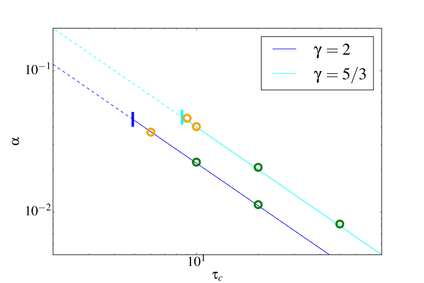
Figure 1: The angular momentum transport coefficient $\alpha$ as a function of $\tau_{c}$ in purely hydrodynamic gravitoturbulent simulations. Green circles represent simulations with no fragments while orange circles represent simulations where one or several transient fragments are observed. The straight lines are the theoretical predictions of Gammie (2001) and the end bars correspond to the critical cooling time below which the disc is fragmenting as a whole.

In order to check our code and compare our results with these previous studies, we performed several simulations without magnetic field ($B_{y_{0}}=0$) and a varying $\tau_{c}$. We used the procedure described in section 2.4.2 to generate suitable initial conditions. Two different adiabatic indices were considered, $\gamma=5/3$ and $\gamma=2$. Simulations that did not fragment into one or few massive clumps were run for at least $600\,\Omega^{-1}$ in order to obtain well-defined saturated states. Fig. 1 shows the average angular momentum transport coefficient $\alpha$ of these turbulent states, defined in section 2.2, as a function of $\tau_{c}$. We show that for both $\gamma=5/3$ and $\gamma=2$, the $\alpha$ coefficient follows the theoretical prediction of Gammie (2001) (indicated by straight lines). As this prediction is derived from an energy conservation principle, this result is just saying that numerical energy losses are small in our simulations. Fig. 1 also shows that these turbulent states collapse into clumps when $\tau_{c}$ is decreased, though the transition is not necessarily well defined, as in Paardekooper (2012). For $\gamma=2$, local and transient fragments appear first for $\tau_{c}=6\,\Omega^{-1}$ while the entire computational domain fragments when $\tau_{c}\lesssim 5\,\Omega^{-1}$. For $\gamma=5/3$, the first fragments appear at $\tau_{c}\lesssim 10\,\Omega^{-1}$ while massive unstable clumps are formed below $\tau_{c}\lesssim 8-9\,\Omega^{-1}$. In both cases, the critical $\alpha_{c}$ for which the disc fragments is comparable and around $\alpha_{c}\simeq 0.04-0.05$.

We found that the average Toomre parameter $Q$ in steady turbulent simulations does not depend strongly on $\gamma$. However it seems to slightly decrease as $\tau_{c}$ is reduced, going from $Q=3$ when $\tau_{c}=50\,\Omega^{-1}$ to $Q=2$ when $\tau_{c}=10\,\Omega^{-1}$. This behaviour is not very surprising: when $\tau_{c}$ is decreased, cooling is enhanced requiring a commensurate increase in turbulent heating by GI, only possible by decreasing $Q$.

3.2 MHD simulations: dependence of the gravito-turbulent state on $B_{y_{0}}$

We first study the ‘ideal case’ in which we do not include any explicit resistivity. We performed a series of simulations by fixing the cooling time $\tau_{c}=20\,\Omega^{-1}$ and the adiabatic index $\gamma=2$, but varying the background toroidal field $B_{y_{0}}$ (or equivalently $\beta_{0}$). We found that for this particular cooling time, all simulations with $\beta_{0}\gg 1$ reach a steady turbulent state without developing massive clumps. Although we started with a pure uniform toroidal field, the geometry of the magnetic field in the nonlinear turbulent regime becomes very intricate and tangled. In some cases, it is amplified and the average gas to magnetic pressure ratio measured in the saturated turbulent regime

$$\beta_{t}=\dfrac{2\left<\Sigma c_{s}^{2}\right>}{\left<B^{2}\right>},$$ (13)

can differ greatly from the initial plasma parameter $\beta_{0}$. In the turbulent state, three different forces emerge in the leading order balance, namely the Lorentz, pressure gradient, and gravitational forces. By varying $\beta_{0}$, we found three different regimes characterised by the relative importance of the Lorentz force with respect to other forces.

3.2.1 First regime: $\beta_{0},\,\beta_{t}\gg 1,\,\,E_{G}\gg E_{m}$

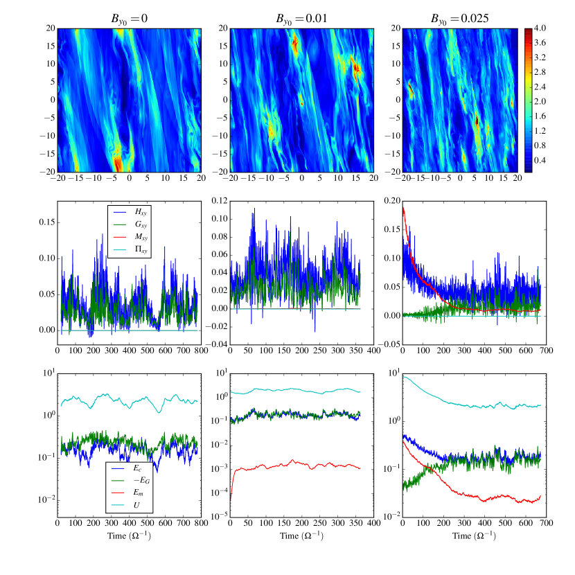
Figure 2: Simulations of gravitoturbulence in the regime $\beta_{0}\gg 1,\,\,E_{G}\gg E_{m}$, computed for fixed $\tau_{c}=20\Omega^{-1}$ and $\gamma=2$. From left to right, $B_{y_{0}}=0$, $B_{y_{0}}=0.01$ and $B_{y_{0}}=0.025$. Top panels: snapshots of the surface density $\Sigma$ in the disc plane ($x$,$y$). Centre panels: the time evolution of the Reynolds ($H_{xy}$), gravitational ($G_{xy}$), Maxwell ($M_{xy}$) and viscous ($\Pi_{xy}$) stresses. Bottom panels: the time evolution of kinetic $E_{c}$, gravitational $-E_{G}$, magnetic $E_{m}$ and internal energy $U$ in a logscale. The simulation in the second column with $B_{y_{0}}=0.01$ was started from a hydrodynamic run. The third simulation, with $B_{y_{0}}=0.025$, was initiated from a MHD run with $B_{y_{0}}=0.05$, which explains why the magnetic energy and Maxwell stress first decrease before reaching a steady state.

The first regime corresponds to the case of a small Lorentz force compared to the gravitational and pressure forces. The magnetic field is completely slaved to the gravito-turbulence and its back-reaction on the fluid motion is insignificant or weak. The field can be stretched or compressed so that it grows until reconnection processes take place and destroy it. Figure 2 shows three different simulations obtained respectively for $B_{y_{0}}=0$, $B_{y_{0}}=0.01$ and $B_{y_{0}}=0.025$ ($\beta_{0}=\infty$, $\beta_{0}=20000$ and $\beta_{0}=3000$). In the case of a weak but non-zero magnetic field, the flow undergoes a transient phase, before it reaches a steady turbulent state. The final state looks much like the hydrodynamic one although turbulent structures appear on slightly smaller scales. The center panels of Fig. 2 indicate that the Maxwell stress is small compared to the Reynolds and gravitational stresses. The time evolution of the energy budget is shown in the bottom panels. It is clear that magnetic energy remains at least an order of magnitude smaller than the other sources and is dynamically insignificant to a first approximation.

Figure 4 shows some key dimensionless quantities averaged in space and time. The Toomre parameter $Q$ remains close to the hydrodynamic value, although it slightly increases from $B_{y_{0}}=0$ to $B_{y_{0}}=0.05$. This result suggests that the temperature regulation and energy balance are only marginally affected by magnetic fields in this regime. We note that $\beta_{t}$, which is directly related to $E_{m}/U$, increases very rapidly as a function of $B_{y_{0}}$, even if it remains much smaller than the other energy ratios.

3.2.2 Second regime: $\beta_{0},\,\beta_{t}>1,\,\,E_{m}>E_{G}$

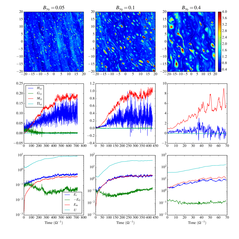
Figure 3: Simulations of gravitoturbulence in the regime $\beta_{0}\gg 1,\,\,E_{m}>E_{G}$, computed for fixed $\tau_{c}=20\Omega^{-1}$ and $\gamma=2$. From left to right, $B_{y_{0}}=0.05$, $B_{y_{0}}=0.1$ and $B_{y_{0}}=0.4$. Top panels: snapshots of the surface density $\Sigma$ in the disc plane ($x$,$y$). Centre panels: the time evolution of the Reynolds ($H_{xy}$), gravitational ($G_{xy}$), Maxwell ($M_{xy}$) and viscous ($\Pi_{xy}$) stresses. Bottom panels: the time evolution of kinetic $E_{c}$, gravitational $-E_{G}$, magnetic $E_{m}$ and internal energy $U$ in a logscale. The simulations shown in the first and second columns were started from the hydrodynamic state while the third was initiated from the MHD steady state obtained for the stronger field run $B_{y_{0}}=0.1$.

For stronger imposed fields we enter a second regime corresponding to when the Lorentz force is comparable to or larger than the gravitational force, but still smaller than pressure gradients. Unlike the first regime, the back reaction of the magnetic field on the fluid motion is no longer negligible. Figure 3 shows three simulations obtained respectively for $B_{y_{0}}=0.05$, $B_{y_{0}}=0.1$ and $B_{y_{0}}=0.4$ ($\beta_{0}=800$, $\beta_{0}=200$ and $\beta_{0}=12.5$). The plots in the center row indicate that the Maxwell stress $M_{xy}$ is now the largest contributor to the total stress and therefore to the angular momentum transport. Although the total stress increases with $B_{y_{0}}$ owing to the new term $M_{xy}$, $\alpha$ remains constant ($\alpha=0.022$) as it only depends on the cooling time (see Gammie (2001)). The magnetic energy is strongly enhanced in this regime and becomes much larger than the background. Figure 4 shows that the ratio between magnetic energy and internal energy increases with $B_{y_{0}}$ and saturates at larger $B_{y_{0}}$. The plasma is close to equipartition between magnetic energy and kinetic energy, as $E_{c}/U$ and $E_{m}/U$ tend to a similar value.

Figure 4 tells us that the internal energy increases significantly with $B_{y_{0}}$ because the average $Q$ and sound speed increase by an order of magnitude between $B_{y_{0}}=0.05$ and $B_{y_{0}}=0.4$. For $B_{y_{0}}=0.1$, the average temperature in the box is multiplied by a factor ten compared to the temperature in hydrodynamic simulations. This surprising result shows that a gravitoturbulent state can exist at values of $Q$ much larger than in hydrodynamics. The greater temperatures are associated with the formation of elongated current sheets and consequent heating at those locations through magnetic reconnection (and associated shocks). The substantial amplification of the background field by the turbulence and its subsequent dissipation provides a powerful and additional source of heat. This is analysed in more detail in section 5.1.

A consequence of this rise in temperature is that the gravitational instability becomes weaker, as indicated by the gravitational stress which clearly decreases by one or two orders of magnitude. Figure 4 shows that most of the gravitational energy present in the small $B_{y_{0}}$ regime has been replaced by magnetic energy. It is then reasonable to ask whether self-gravity is important at all in this state. To check that, we ran a simulation starting from developed gravitoturbulence and then switched off the gravitational term. We found that as soon as self gravity is suppressed, the turbulent kinetic and magnetic energy decay to negligible levels by $t\sim 100\,\Omega^{-1}$. This indicates that self-gravity, however weak it is, still plays a crucial role in sustaining the turbulence.

The fact that graviturbulent activity persists for such large $Q$ may have something to do with the relaxation of angular momentum conservation by the magnetic stresses. It is likely that transport via a tangle of magnetic fields weakens the stabilising effect of rotation, permitting GI to operate for larger $Q$. A similar effect is witnessed when explicit viscosity is included in the linear theory (e.g. Schmit & Tcharnuter 1995) and probably in the nonlinear onset of GI. It should be acknowledged that in pure hydrodynamics it is not yet understood what sets the level of the saturated $Q$; adding a magnetic field must further complicate the problem.

The top panels in Fig.  3 show that the plasma is characterized by dense clumps whose size are comparable to or smaller than $H_{0}$. These ‘plasmoids’ are associated with magnetic island structures and evolve in a turbulent background that resembles the hydrodynamic state (non-axisymmetric waves amplified transiently and dissipated into shocks). These plasmoids appear to resist the shear and the shocks that propagate through them. A detailed analysis of these structures is provided in section 5.2. Note that the magnetic islands are reminiscent of compressible turbulent 2D MHD simulations in which a forcing term is included (Lee et al., 2003).

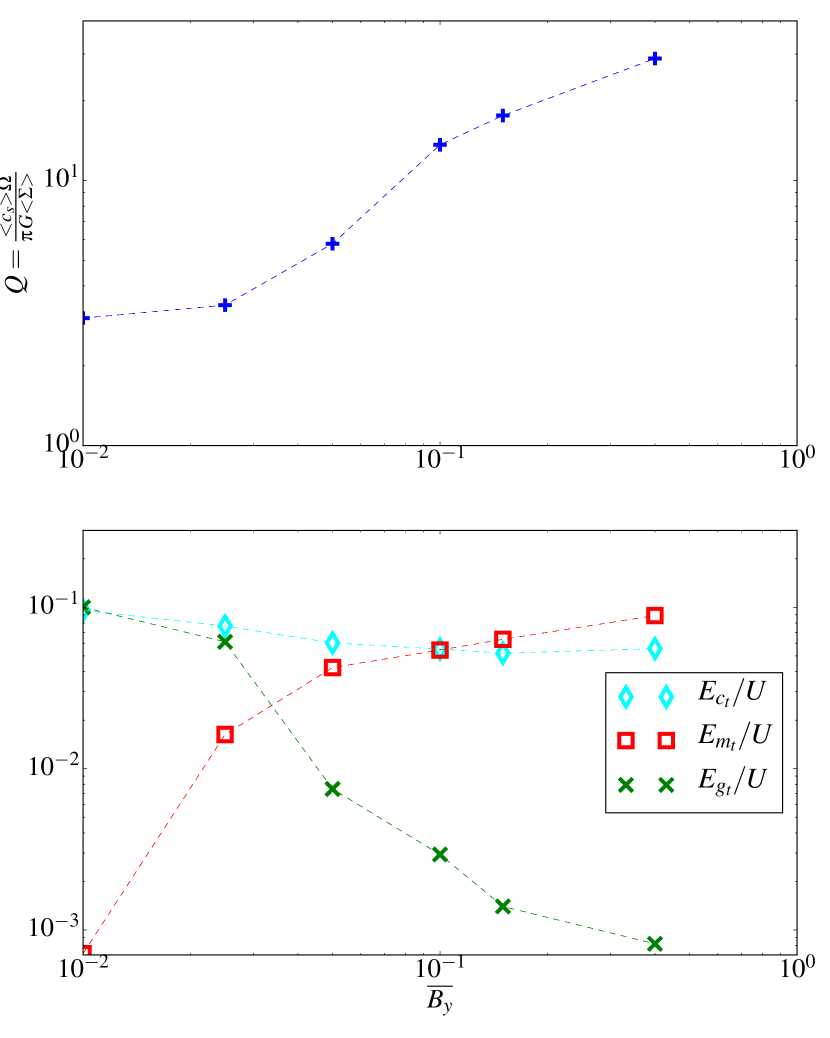
Figure 4: Top panel: the average Toomre parameter $Q$ as a function of $B_{y_{0}}$. Bottom panel: ratios of kinetic, magnetic and gravitational perturbation energy to the total internal energy for different $B_{y_{0}}$. The yellow dashed line is the turbulent angular momentum transport coefficient $\alpha$. All these simulations have been computed for a fixed $\tau_{c}=20\,\Omega^{-1}$ and a fixed adiabatic index $\gamma=2$.

3.2.3 Third regime: $\beta_{0},\,\beta_{t}\leq 1,\,\,E_{m}\gg E_{c}$

As we approach $\beta_{0}=1$, the fluid becomes magnetically dominated and the gravitational term is reduced. For $\beta_{0}=1$ and $\beta_{0}=0.5$, which correspond probably to an unrealistic regime for astrophysical discs, our simulations show that the fluid motion is completely frozen into the magnetic field lines and unable to move due to strong magnetic tension. The toroidal field acts like a ‘straightjacket’, and steady turbulent states cannot be achieved. Flux tubes with a coherent radial length larger than the non-axisymmetric gravitational structures develop and sometimes form regions of high density that collapse rapidly after a few orbits. These structures are very similar to those obtained by Lee et al. (2003). We note that this regime is extremely challenging numerically, especially with our fine resolution, since the time step becomes very small.

3.3 Fragmentation criterion

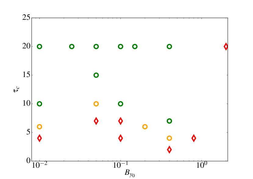
Figure 5: Fragmentation criterion as a function of the cooling time and $B_{y_{0}}$. Green circles indicate simulations that do not fragment at all. Orange circles indicate simulations that remain turbulent but for which one or several transient fragments are observed. Red diamonds correspond to simulations where the disk collapses into one or a few massive clumps.

In this section we vary the cooling time $\tau_{c}$ in order to study the onset of fragmentation. Each simulation is run for $100\Omega^{-1}$. For all values of the background field $B_{y_{0}}$, there is a critical $\tau_{c}$ below which the disc collapses into massive clumps (within the simulation time). Figure 5 shows how this critical $\tau_{c}$ varies with $B_{y_{0}}$. In the first regime, $E_{G}\gg E_{m}$, the critical cooling time is multiplied by a factor $\sim 2$ between $B_{y_{0}}=0$ and $B_{y_{0}}=0.05$. Weak magnetic tension helps fragmentation by extracting extra angular momentum from within a potentially collapsing region, thus thwarting the Coriolis force.

In contrast, the plasmoid-dominated regime, $E_{m}\gtrsim E_{G}$, witnesses an unexpected decrease in the critical cooling time with $B_{y_{0}}$. This is probably due to the enhanced heating generated in the presence of a stronger imposed field. An increased magnetic field causes the gas to be signifcantly hotter, as explored in the previous subsection. The associated pressure prevents fragmentation and overwhelms the direct destabilising effect of the magnetic field in collapsing a plasmoid, via magnetic tension and pressure.

Overall, the relative variation of the critical cooling time with $B_{y_{0}}$ remains small, which suggests that magnetic fields, despite their strong influence on the turbulent properties, do not dramatically change the fragmentation criterion. Note that, similarly to the hydrodynamical case, the average $Q$ decreases when $\tau_{c}$ is decreased ($Q\sim 30$ for $\tau_{c}=20$ and $Q\sim 18$ for $\tau_{c}=7\,\Omega^{-1}$ in the case of $B_{y_{0}}=0.4$). No criterion for fragmentation depending on $\alpha$ or $Q$ can be obtained simply in that case.

4 Effects of resistivity

Up to now we have explored only ‘ideal’ MHD — the particulars of the grid have been taking care of the reconnection, diffusion, and thermalisation of magnetic field. In this section we include magnetic resistivity explicitly to better control this process and also to push our models to regimes relevant to the more resistive radii in protoplanetary disks. We find that increasing diffusion, unsurprisingly, impedes the build up of the strong fields witnessed in section 3.2; the field slips through the turbulent gas and is no longer wound up, stretched, and amplified as efficiently.

In protoplanetary discs, the magnetic Reynolds number Rm is directly proportional to the gas’s ionisation fraction, which is determined by interparticle collisions, cosmic rays and X-rays, radioisotopes, molecular recombination, and dust grain physics (Armitage, 2011). In a minimum mass solar nebula (MMSN) model, estimates for the midplane Rm vary from $\sim 0.1$ at 5 AU to $10^{3}$ at 10 AU, to greater than $10^{4}$ at larger radii (Simon et al., 2015). In fact, both ambipolar diffusion and the Hall effect are more important than Ohmic diffusion at the latter two radii. The equivalent ambipolar magnetic Reynolds number is defined as $R_{A}=\Omega H^{2}\nu_{in}\rho^{2}x_{e}/B^{2}$ where $\nu_{in}$ is the ion-neutral collision rate and $x_{e}$ is the ionisation fraction. This number varies roughly between 0.1 to 10 times $\beta$ between 5 and 100 AU (e.g. Simon et al., 2015). If we are permitted to crudely model ambipolar diffusion by Ohmic diffusion in our simulations, then our effective Rm should take values between 1 and $10^{4}$.

The reader should be aware, however, that the above estimates for non-ideal MHD were derived with the MMSN model, which best describes an older type-II disk, which is insufficiently massive to suffer GI. The relative strengths of Ohmic and ambipolar diffusion will differ in a GI-unstable type-0 system, which will be denser (hence the ions and neutrals better coupled) but also less well-ionised because optically thicker. The above estimates hence only serve as a rough guide, to fix ideas.

An additional complicating factor is that the ionisation fraction (and hence Rm and $R_{A}$) depends on height, and so the gas at different vertical levels is not coupled to the magnetic field in the same way. These issues make it less than straightforward to assign a simple Ohmic diffusivity to 2D simulations, and in fact to interpret the role of diffusion in two dimensions generally.

One other extremely important ingredient, neglected in our work, is the MRI. Though absent in the heart of dead zones $\sim 5$ AU, it may appear in the more favourable ionisation conditions at larger radii, though the details of its prevalence are exceptionally complicated and the subject of intensive research. The outcome depends not only on the (poorly constrained) ionisation profile, but on the orientation, strength, and existence of a net magnetic field, with simulations showing that the midplane can be completely laminar, undergo bursts of turbulence, or sustain a sluggish form of the MRI. The surface regions, on the other hand, may launch a magnetocentrifugal wind or suffer vigorous turbulence (Simon et al., 2013, 2015). We cannot hope to adequately model this physics in our 2D simulations, but hope that its diffusive aspects can be roughly described by a constant resistivity.

$B_{y_{0}}=0.05$ i.e $\beta_{0}=800$ Rm $Q$ $E_{m}$ $E_{m}/U$ Plasmoids 0 (hydro) 3.02 x x x 10 3.16 0.0011 0.002 NO 100 3.2 0.005 0.0026 NO 500 3.4 0.025 0.012 NO 1000 4.9 0.16 0.031 YES (very few) 5000 5.7 0.27 0.037 YES ideal approx. 5.8 0.36 0.042 YES

$B_{y_{0}}=0.1$ i.e $\beta_{0}=200$ Rm $Q$ $E_{m}$ $E_{m}/U$ Plasmoids 0 (hydro) 3.02 x x x 100 3.1 0.024 0.012 NO 250 7.6 0.28 0.026 YES (very few) 500 10.9 0.84 0.035 YES 1000 12.5 1.35 0.045 YES 5000 (hlld) 13.6 1.78 0.05 YES ideal approx. 13.7 1.88 0.053 YES

Table 1: Average $Q$, magnetic energy, and the ratio of magnetic to internal energies for different Rm. The first table corresponds to simulations with $B_{y_{0}}=0.05$, and the second to $B_{y_{0}}=0.1$. The last column indicates whether plasmoids appear. All simulations were conducted with the hll solver except for $\text{Rm}=5000$ and $B_{y_{0}}=0.1$ which was undertaken with the hlld solver.

4.1 Resistive turbulent simulations

To determine the effect of Ohmic diffusion on MHD gravito-turbulent states, we performed a series of simulations with explicit resistivity by taking a fixed $B_{y_{0}}$ and varying the magnetic Reynolds number. We scanned a large range of Rm, straddling midplane values typical of dead zones and larger radii. Our simulations were initiated from a saturated state computed in the ideal limit and run until a new steady state was found.

Table 1a) sums up the different results obtained for $B_{y_{0}}=0.05$ (equivalently $\beta_{0}=800$). As expected, when $\text{Rm}=5000$ the turbulent state differs little from the ‘ideal case’ because the numerical and physical Rm are of the same order. For such values of Rm, Ohmic diffusion is probably unresolved. However, the statistical properties of the turbulence change quite drastically when $\text{Rm}\lesssim 1000$. For this transitional Rm, the magnetic energy is roughly halved while $Q$ drops to 4.9 (from 5.8). Another change is that the number of plasmoids in the box is considerably reduced while their typical density decreases by a factor 4. Below $\text{Rm}=500-1000$, plasmoids structures disappear and $Q$ approaches its hydrodynamical value. At these Rm, diffusion impedes the build up of large magnetic energies (that may be subsequently thermalised) and the disk is hence cooler. Results for a stronger imposed field $B_{y_{0}}=0.1$ ($\beta_{0}=200$) are presented in Table 1b). Now the magnetic energy and $Q$ decrease sharply around a lower critical $\text{Rm}\sim 100-250$, and plasmoid structures disappear for $\text{Rm}\lesssim 250$.

To conclude, the main effect of resistivity is to reduce the average turbulent magnetic energy stored in the fluid. As a consequence, there is less free energy to be dissipated into heat and the mean temperature decreases. Below some critical $\text{Rm}_{c}$ that seems to scale as $\beta_{0}$, the turbulence becomes decoupled from the magnetic field. This result suggests that a key quantity to study the transition between ‘quasi-hydrodynamical’ and plasmoid-dominated MHD turbulence might be the Elssaser number $\Lambda\sim\text{Rm}\,\beta_{0}^{-1}$.

4.2 Zero net flux simulations and decay rate

As mentioned in section 2.4.2, a 2D turbulent flow cannot sustain a dynamo field, which means that if we start with a zero net toroidal flux, the magnetic field is expected to decay within a finite time. However, the decay time can be exceptionally long, due to compressibility, the geometry of the initial field, and a large Rm (see also Ivers & James 1984). It may even be possible to sustain a magneto-turbulent state throughout a great fraction of a disk’s life. To give an estimate of the decay timescale, we performed two different simulations with zero net flux. In the first one, labelled ‘Zs’, we started from a state computed with $B_{y_{0}}=0.1$, removed the mean component of the toroidal field and then let the flow evolve in time. In the second one, labelled ‘Zl’, we started from the same state but we added at $t=0$ a sinusoidal $B_{y_{0}}\propto\sin(2\pi/L_{y})$ with an energy equivalent to the one with uniform background field. Both simulations were performed with explicit resistivity and $\text{Rm}=5000$. In the Zs case, the magnetic energy $E_{m}$ decays to negligible values by 150 $\Omega^{-1}$, which corresponds roughly to the decay time expected. Indeed if the turbulent magnetic structures are of scale $\sim H_{0}$, then the resistive decay time is given by $H_{0}\,\text{Rm}/4\pi^{2}\sim 126\,\Omega^{-1}$. In the Zl case, we found however that the initial magnetic field is retained over at least $1000\,\Omega^{-1}$ while magnetic energy stays virtually constant throughout the simulation. This is expected because the estimated decay time for the large-scale $B_{y_{0}}$ is of the order $2\times 10^{5}\,\Omega^{-1}$, comparable or longer than the disc viscous timescale.

5 Current sheets and plasmoids

5.1 Heat sources and currents sheets

We showed in section 3.2 that for intermediate $B_{y_{0}}$, the Maxwell stress produces a large contribution to the total stress and provides an additional source of thermal energy. The build up of magnetic energy is another source, once it is dissipated via current sheets or related structures (Parker, 1972; Cowley et al., 1997). As the heat generated by magnetic fields drastically alters the thermodynamic state of the turbulence, and in particular the average $Q$, it is crucial to better understand it.

5.1.1 Mean features

To identify the main source of heat in our MHD simulations, we investigated the relative importance of each term in the averaged equation for internal energy:

$$\dfrac{d\langle U\rangle}{dt}=\langle-P\nabla\cdot\mathbf{u}\rangle+\langle D_{\nu}+D_{\eta}\rangle-\langle U\rangle/\tau_{c}.$$ (14)

Physically, the heat can be generated through two different processes: reversible compression or expansion of the gas which is associated with the term

$$W_{PV}=-P\nabla\cdot\mathbf{u},$$ (15)

and irreversible dissipation like viscous and Ohmic friction, whose dissipation rates are respectively:

$$D_{\nu}=\boldsymbol{\Pi}:\mathbf{\nabla v}\quad\text{and}\quad D_{\eta}=\eta\left(\nabla\times\mathbf{B}\right)^{2}.$$ (16)

The main difference between these sources is that pressure work $W_{PV}$ (also called ‘pressure-dilatation’) can have either a positive or negative sign, meaning that the energy transfer between kinetic and thermal modes can be in either direction. In contrast, irreversible processes transfer energy from the kinetic to thermal channels only.

We analysed the net heat budget for $B_{y_{0}}=0.1$ and Rm $=500$ by averaging eq. (14) in time over $150\Omega^{-1}$. We found that almost 45% of the budget is represented by pressure work $W_{PV}$, 20% by the Ohmic term $D_{\eta}$ and 6% by the viscous term $D_{\nu}$. The leftover is taken up by numerical dissipation. Note that when a HLLD solver is used, the viscous term becomes 11% but the average $Q$ and temperature are unchanged. The rather significant amount of numerical dissipation is not surprising and arises because of the presence of thin shocks layers which are difficult to resolve viscously. However, as discussed in section 2, only a tiny fraction of energy is lost, the numerical dissipation is mostly recycled as heat in a way approximating real microscopic dissipation inside a shock.

A notable result is that a large fraction of the heat comes from the reversible expansion of the gas through the pressure dilatation term $W_{PV}$, which oscillates between positive and negative values, with a frequency $\approx\Omega$ but which is positive on average. In most studies, this reversible heating is considered irrelevant because a fluid parcel in the disc is thought to relax adiabatically and return to its unperturbed state shortly after the passage of a spiral wave or a shock (e.g., Rafikov, 2016). On average, the heat generated through an expansion is removed by a subsequent relaxation because there is a similar degree of compression and expansion in the gas ($\langle\nabla\cdot\mathbf{u}\rangle=0$). This is true when the gas can relax adiabatically on a timescale much shorter than the cooling time, and when a gas parcel encounters waves or shocks on a timescale longer than the adiabatic relaxation time. In our simulations neither need be the case. The fluid endures a turbulent forcing so strong that it has no time to relax between each compression or shock crossing. A similar net reversible compressible energy transfer, due to pressure dilatation, has been observed in 2D and 3D hypersonic compressible turbulence, with no radiative cooling, in a separate non-disk context (Zeman, 1991; Sarkar, 1992). In particular, for shear flows, this transfer can be comparable to the compressible viscous dissipation term and contributes to a reduced growth of turbulent kinetic energy when the flow is integrated over a long time (the missing part being transferred to internal energy).

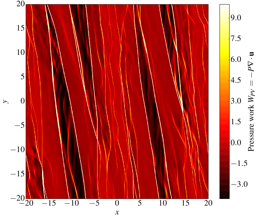
Figure 6: A snapshot of the distribution of pressure dilatation $W_{PV}$ in hydrodynamic gravitoturbulence ($B_{y_{0}}=0$). Bright and white colors indicates heating by compression, dark and black indicates region where the gas expands and relaxes. The intensity has been intentionally saturated at $W_{PV}=10$ but the real maximum is $W_{{PV}_{max}}\sim 150$.

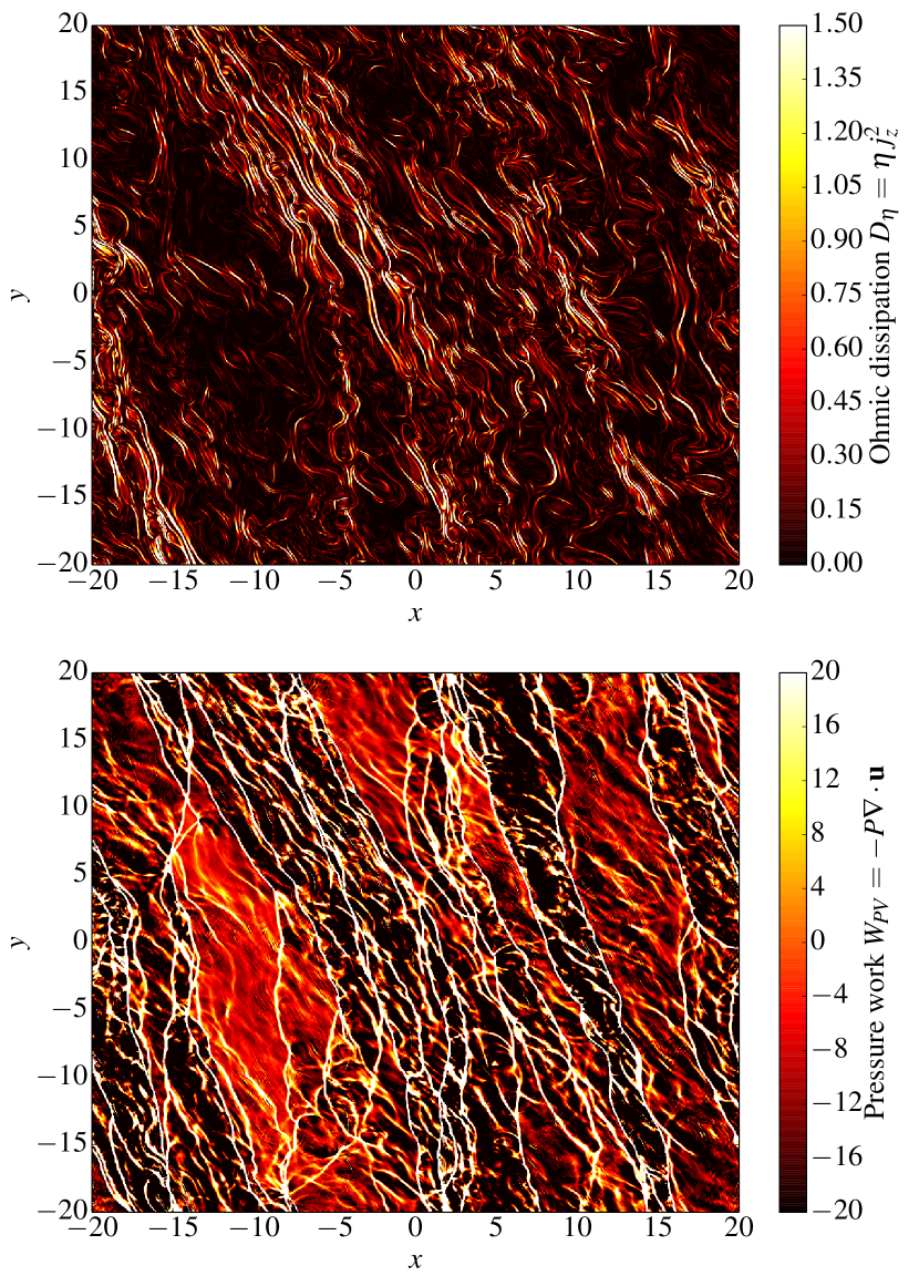
Figure 7: Heat sources in a quasi-steady turbulent state obtained for $B_{y_{0}}=0.1$ and $\text{Rm}=500$. The top panel represents the Ohmic dissipation $D_{\eta}$ whereas the bottom panel represents the pressure dilatation $W_{PV}$. The intensity has been intentionally saturated at $W_{PV}=20$ but the real maximum is $W_{{PV}_{max}}\sim 5000$, much greater than in hydrodynamical runs.

5.1.2 Dissipative structures

In addition to the average budget for the internal energy, we analysed the spatial distribution of the heat sources in the hydrodynamic case and in a magnetized gravito-turbulent flow with $B_{y_{0}}=0.1$. Figure 6 shows that when $B_{y_{0}}=0$, the main sources (here the reversible part) are located in very thin azimuthally elongated structures. These thin layers correspond to shock waves that propagate within the fluid and are associated with the nonlinear evolution of large-scale gravitational wakes. The black/dark regions correspond to expanding gas ($\nabla\cdot\mathbf{u}>0$) where the pressure is found to be maximum.

Figure 7 presents a snapshot from a magnetic simulation. The second panel shows again that the pressure work is concentrated into very thin filaments, which reveal the location of shocks, but their geometry is tremendously more complicated and their number clearly increased. In comparison with the hydrodynanical case, the surface covered by these heat sources is multiplied by a factor $\sim 10$, for $B_{y_{0}}=0.1$ (this is estimated by computing the surfaces where $W_{PV}>10$). These intricate patterns reveal also that the heat transfer is concentrated in smaller scale structures, with a typical length that seems correlated to the size of the magnetic field bundles.

Although we showed that Ohmic dissipation is not the dominant source of heat directly, its associated current sheets might play a crucial indirect role by generating shocks. Figure  7a) shows the regions where magnetic energy is dissipated into heat via Ohmic dissipation. These regions clearly take the form of filamentary structures with a small azimuthal extent (compared to $L_{y}$). There appears to be a correlation between the number of such sheets and the number of shocks for which $W_{PV}$ is positive. In addition, the location of these structures seems to be found in regions of high pressure, where $\nabla\cdot\mathbf{u}$ is actually a minimum. These regions correspond to the self-gravity wakes that take the form of large scale non-axisymmetric bands.

Magnetic reconnection in current sheets is known to accelerate the gas, producing sometimes a pair of slow-mode shocks extending outwards from the central sheet (Petschek, 1964; Priest & Forbes, 1986; Birn & Priest, 2007; Hillier et al., 2016). These shocks are known to be highly effective at heating the surrounding medium. In fact, some numerical studies indicate that the slow mode shocks are the primary heating mechanism in the solar corona (Bareford & Hood, 2015). In some circumstances the energy released from these shocks can be more important than Ohmic dissipation, as seems to be the case here. Though we do not go into a detailed analysis in this paper, it seems plausible that the enhanced heating witnessed by magnetic gravitoturbulence is caused by Ohmic reconnection in current sheets and in the shocks generated by such reconnections.

5.2 Plasmoids

As pointed out in section 3.2.2, when magnetic fields have a moderate amplitude and Rm is not too small, the turbulent flow displays coherent plasmoid structures and magnetic islands. These patterns have been studied exhaustively in the literature of magnetic reconnection (Park et al., 1984; Ugai, 1995; Loureiro et al., 2005; Huang & Bhattacharjee, 2013; Loureiro & Uzdensky, 2016) and 2D compressible MHD turbulence (Lee et al., 2003) but have not featured especially in simulations of accretion disc dynamics. In this context they deserve further attention as it is tempting to associate them with planet formation, possibly as sites in which dust may accumulate. Separately, an examination of their intrinsic balances and structure may help unveil the role of the Lorentz force in magnetized shear flows generally.

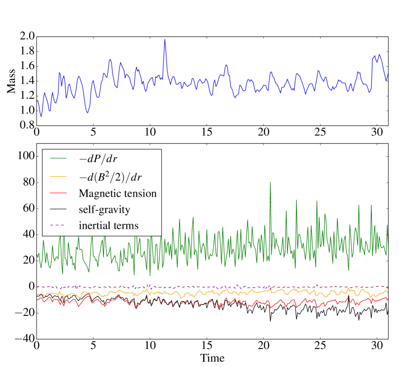
Figure 8: Top panel: evolution of the total mass in a plasmoid computed from a simulation with $B_{y_{0}}=0.05$ and no explicit resistivity. Bottom panel: radial forces integrated over the interior of the plasmoid in a frame of reference centered at the pressure maximum. The typical radius of the plasmoid (taken as our integral bound for averaging) is $r_{p}=0.4H$.

5.2.1 Are they fragments?

The first question is what relationship these magnetic islands have with respect to the gravitationally bound fragments that appear in hydro simulations of GI. Figure 8 (top) shows that, for $B_{y_{0}}=0.05$ and $\tau_{c}=20/\Omega$, the total mass integrated inside one of the plasmoids does not increase with time and keeps a fixed value during more than 30 $\Omega^{-1}$. Actually, we checked visually that they stay stable over a much longer time. Although they form dense structures with $\Sigma$ that can exceed 50 times the background $\Sigma_{0}$, they do not seem to be regions where the gas is collapsing, at least for sufficiently large $\tau_{c}$. We conclude that they are resolved quasi-steady objects quite different to the fragments seen in hydrodynamical simulations of gravitational collapse.

5.2.2 Origins

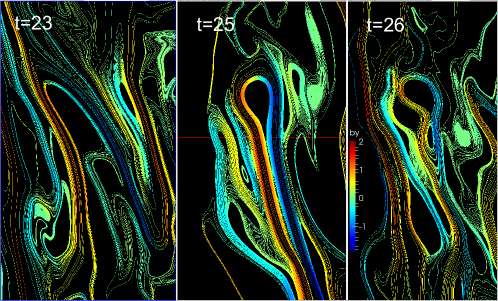
Figure 9: Three snapshots showing the evolution of the magnetic field line topology in a small patch centred around a region of plasmoid formation over a period of $3\,\Omega^{-1}$. Blue represents negative field polarity, while represents positive $B_{y}$. The intensity of the colour quantifies the magnitude of the field. The $x$-extent of the patch is $3H_{0}$, while the $y$-extent is $5H_{0}$.

In order to understand how plasmoids form, we investigated the early stages of a simulation in which magnetic islands appear. We found that this stage occurs just after the onset of the turbulence. Figure 9 shows the field line configuration near a plasmoid forming region between $t=23\,\Omega^{-1}$ and $t=26\,\Omega^{-1}$ for $B_{y_{0}}=0.1$. Initially straight azimuthal field lines are stretched, folded and amplified by the turbulent eddies. Strong positive (red) and negative (blue) toroidal magnetic fields are then brought together. At $t=25\,\Omega^{-1}$, a current sheet is forming as soon as the magnetic loop is closed. At $t=26\,\Omega^{-1}$, the field lines become possibly unstable to the tearing instability (Biskamp, 1986; Loureiro et al., 2005) and reconnect, forming two magnetic islands. These snapshots (and many others like them) suggest that plasmoids are generated through a common physical mechanism and are not produced artificially by the code.

5.2.3 Equilibrium and structure

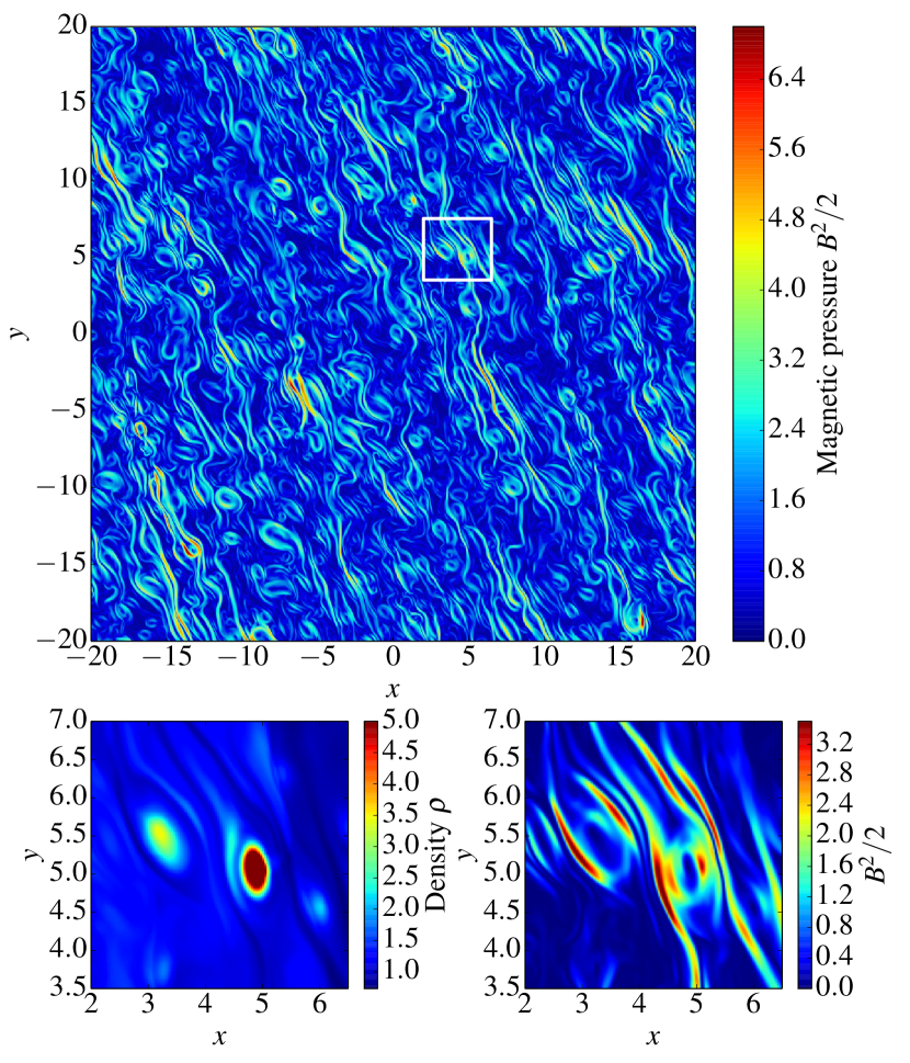
Figure 10: Top panel: total magnetic pressure in a quasi-steady turbulent state obtained for $B_{y_{0}}=0.05$ and no explicit resistivity. The bottom left and right panels are respectively the density and magnetic pressure in the white rectangle appearing in the top panel.

Figure 10 shows a snapshot of a simulation computed for $B_{y_{0}}=0.05$ with no explicit resistivity, containing a number of plasmoids. Magnetic pressure forms strong ring-shape structures surrounding each of these plasmoids that prevent the external gas from penetrating within. To a first approximation they behave as steady rigid bodies in a sheared turbulent background. Some of them are spinning with a net negative vorticity (in the same direction as the shear) but their velocity profile can be quite intricate inside.

Gas pressure and density are always maximum at their centres and decay quasi-exponentially with distance to this axis. Plasmoids are cold and their temperature is minimum at their centres. In order to better understand their internal structure, we computed their force balance. We chose one of our simulation with $B_{y_{0}}=0.05$ and tracked a number of plasmoids by calculating their position and velocity at each output time. Forces are then computed in a particular frame of reference, centred upon a given plasmoid (where the density is maximum). We used polar coordinates around this origin so that $r$ denotes the distance to the center of a plasmoid and $\theta$ the angle with the $x$ axis. Each force is averaged inside the plasmoid by integrating in $r$ and $\theta$. We defined the radial extent of a plasmoid as the radius at which the density has dropped by a factor 2 from its center.

We identified one big plasmoid where the density contrast between the background turbulent flow and the center is $\Delta=0.13$. Fig. 8 shows the radial force balance in the frame of this structure. Inside the plasmoid, the fluid is in equilibrium between the pressure gradient (which is positive and resisting the collapse) and all other forces (that are negative and tend to make the gas collapse). The latter are all of the same order of magnitude although magnetic pressure is roughly half the magnetic tension and self-gravity. Note that inertial forces (Coriolis and nonlinear advection) affect the equilibrium only weakly, indicating that the pressure maxima is not maintained by vortical motions. The plasmoids hence should not be regarded as vortices. (We did not plot the viscous force as it is completely negligible.) Finally, we checked that this force balance is similar for several other plasmoids.

Figure 3 indicates that the plasmoids sizes increases with $B_{y_{0}}$. On one hand, this behaviour might be surprising as we explained that magnetic forces seem to push the gas inward and force the structure to contract. But on the other hand, for the same reason as explained in Section 3.3, the pressure increases very rapidly with $B_{y_{0}}$, due to the heat generated by magnetic fields in this regime. In addition, the gravitational force becomes less important in comparison with pressure forces as $Q$ is increased. Therefore, a balance is still possible and the size of the structures can even grow with $B_{y_{0}}$.

6 Discussion and Conclusion

In summary, we performed 2D shearing sheet simulations of gravitoturbulence in magnetised accretion disks penetrated by a net toroidal field. For moderate plasma beta and magnetic Reynolds number, this field was twisted, warped, and greatly amplified by the turbulent velocity fluctuations. Once a quasi-steady state was achieved the final magnetic energy could, in fact, be equal to the turbulent kinetic energy. Once thermalised, this additional reservoir of energy leads to a dramatic heating of the gas, and enhanced quasi-equilibrium temperatures (and thus Toomre $Q$’s). For example, when $\beta_{0}\sim 100$ and Rm$>1000$, the mean $Q$ is amplified over the hydrodynamic value by a factor 4. For the same $\beta_{0}$ but a larger Ohmic resistivity, Rm$=250$, the amplification is a factor 2. The system can thus achieve a marginal gravitoturbulent state in which $Q\sim 20$, and the gravitational potential energy subdominant (though absolutely necessary for the subsistence of the steady state). For lower Rm or weaker imposed fields these striking effects subside and the system begins to resemble the hydrodynamical regime. We tentatively attribute the persistence of GI activity at such high $Q$ to the breaking of angular momentum conservation by the tangled magnetic field. The suppression of this stabilising effect exacerbates the GI and extends the range of gravitoturbulent activity to hot states where it would ordinarily be stable.

The thermalisation of the magnetic energy is undertaken through the action of small-scale current sheets, and especially the slow shocks generated by reconnection in the sheets. The resulting heating is highly inhomogeneous and localised in an intricate network of shock layers. The temperature fluctuations in this network may greatly exceed the mean temperature of the disk, and may have some consequences for chemistry and the processing of solids (see for example, Godard et al. (2009) or McNally et al. (2014)). For sufficiently large Rm, reconnection also generates plasmoids, long-lived magnetic islands distinct from both vortices and gravitationally collapsing blobs. If shown to be prevalent and robust, these structures could be of interest to planet formation theories.

Finally, we checked to see if magnetic fields had any impact on the fragmentation criterion. By varying the cooling time, for different imposed fields, we obtain critical $\tau_{c}$ below which the gas fragments. In general, these critical values are not very different to the hydrodynamical ones. Given the numerically dependent and stochastic nature of fragmentation, it is difficult to set much store on these results — though the basic idea (that magnetic fields are not so important) may be robust.

Our 2D ideal and resistive simulations are potentially relevant for protostellar disk regions that are magnetically active but MRI stable. As shown in vertically stratified simulations with the full panoply of non-ideal MHD, such regions may span a significant range of outer radii. Strong horizontal fields may be generated by the Hall effect, and winds launched at the disk surfaces. Our numerical set-up does not correctly capture these non-ideal effects, but nonetheless some of the behaviour we witnessed might cross over. An additional uncertainty, in any case, is the correct non-ideal regime for the outer radii of gravitationally unstable class-0 disks. Previous work, and our estimates, have been based on the less massive MMSN model.

Our simulations may also be relevant for massive deadzones in older disks, at the onset of GI-instigated outbursts. The newly GI active region, if supplied by sufficiently strong magnetic fields (by advection from larger radii or locally by Hall currents) could more effectively heat the gas, as described above and thus more easily kickstart the classical MRI, as required by certain outburst models. That said, this enhanced heating requires somewhat larger Rm than typically supported by dead zones, and may only be effective at the outer edge of the zone.

A final application of these results may be to the outer part of AGN discs which are likely to be gravitationally unstable (Paczynski, 1978), and susceptible to fragmentation (Goodman 2003, Levin 2007). Gravitational collapse of the disk may be especially important in star formation bursts close to the Galactic centre. Meanwhile, the AGN gas can be relatively well ionised and able to couple to any latent magnetic field; indeed the MRI and GI may overlap at certain radii in especially luminous systems (Menou & Quataert 2001).

These exploratory 2D results point to a number of future research directions. For a start, Ohmic diffusion could be replaced by ambipolar diffusion to test how magnetic fields behave in the regimes more relevant for the outer radii of protostellar disks. However, the most interesting avenues involve 3D vertically stratified boxes, which could include the $z$-dependent diffusivities and the various interesting non-ideal MHD behaviours recently discovered (Lesur et al., 2014; Bai, 2014; Simon et al., 2015). The latter would then provide magnetic fields self-consistently. Such simulations would let us probe how the gravitoturbulence works in the presence of MHD winds, surface turbulence, and its action on the magnetic field. And though numerically intensive, they would also provide a way to simulate both the MRI and GI together and determine if the two instabilities coexist or attempt to switch each other off.

Appendix A Test of the linearised problem

A.1 Axisymmetric case (isothermal)

We present in this appendix several tests to check that our self-gravity module in PLUTO is correctly implemented. A first test concerns the linear axisymmetric modes. By linearising the system of equations (2)-(5) and assuming that perturbations are of the form $\exp(\text{i}k_{x}x+\text{i}k_{y}y-\text{i}\omega t)$, one can derive a dispersion relation which writes, in the isothermal, inviscid and unmagnetized case

$$\gamma^{2}\equiv-\omega^{2}=-(k_{x}^{2}c_{s}^{2}+\kappa^{2}-2k_{x}\kappa c_{s}/Q).$$ (17)

If the Toomre parameter $Q={\kappa c_{s}}/{\pi G\Sigma_{0}}<1$, then there exists a range of wavenumbers for which the motion is unstable.

$$\dfrac{\kappa}{c_{s}}\left(\dfrac{1}{Q}-\sqrt{\dfrac{1}{Q^{2}}-1}\right)\leq k_{x}\leq\dfrac{\kappa}{c_{s}}\left(\dfrac{1}{Q}+\sqrt{\dfrac{1}{Q^{2}}-1}\right)$$ (18)

To check this relation numerically, we considered a wave in a sheet of size $L_{x}=L_{y}=2\pi$ with a background density $\Sigma_{0}=1$. We assume an isothermal gas ($c_{s_{0}}=1$) and introduce at $t=0$ a perturbation with wavenumbers $k_{x}=2\pi/L_{x}$ and $k_{y}=0$ so that it is marginally unstable for $Q=1$. We perturbed the background along the dominant eigenvector of the linearised problem, ensuring that the evolution of the wave is strictly exponential when the motion is unstable. The initial amplitude is $10^{-5}S\,H$. We have simulated the evolution of these perturbations for different values of $Q$. Figure 11 shows the numerical growth rates $\gamma$ as a function of $Q$, obtained for $Q<1$ and the frequencies $\omega$ obtained for $Q>1$ (red stars). The blue and green lines represent these quantities obtained analytically from equation 17. The relative error between the theoretical and numerical growth rates remains smaller than 0.008 and on average equal to 0.005.

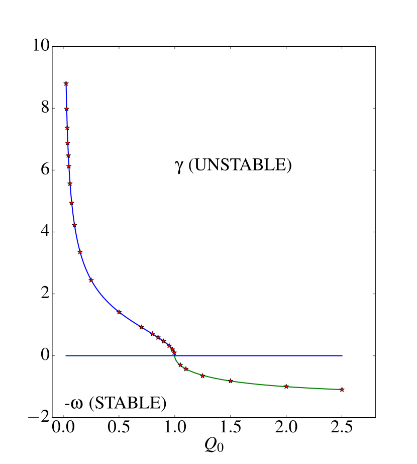
Figure 11: Stability of axisymmetric modes in the local Cartesian thin disc. Solid lines are the theoretical growth rates (positive ordinates) and frequencies (negative ordinates). Red stars are the values obtained with our self-gravity module (working with PLUTO). The resolution is 512 points per azimuthal wavelength.

A.2 Non-axisymmetric case

We performed similar tests for non-axisymmetric waves ($k_{y}\neq 0$). Because these waves have a wavenumber $k_{x}=k_{x_{0}}+Sk_{y}t$ that increases linearly in time, analytical solutions are not straightforward to obtain. They are rapidly sheared out and their evolution on long time scale cannot be described by exponentials. However, it is still possible to solve numerically the linearised problem with a simple Runge Kutta time-stepping algorithm and compare the results with the solutions obtained numerically with PLUTO.

We considered a leading wave with $k_{x}=-4\pi/L_{x}$ and $k_{y}=2\pi/L_{y}$ in a box of size $L_{x}=L_{y}=2\pi$. We tested 3 different configurations by fixing $Q=1.1358$, $\Sigma_{0}=1$, $c_{s_{0}}=1$ and the random initial amplitudes of the velocity and density perturbations. In the first case, the equation of state is isothermal and the gas is unmagnetized. In the second case, $\mathbf{B}=0$ but the energy equation is taken into account. The last configuration accounts for an ideal and magnetized gas, in which a constant magnetic background $B_{x}=0.15$ and $B_{y}=0.3$ is introduced.

The results are shown in Fig. 12, where blue curves represent the evolution of shearing waves simulated with PLUTO and the green one with the linearized solver. Our code reproduces quite well the desired solution during the first shearing times but the waves diffuse at longer times ($t>10\,\Omega^{-1}$) as they are strongly sheared out and damped by numerical diffusion. The resolution used here is $512\times 512$ and we checked that doubling the resolution clearly improves the results. Including an explicit viscosity with Re $=1000$ reduces the numerical diffusion. The diffusion of shearing waves by a Godunov scheme has been already pointed out by Paardekooper (2012). Note that in his case, for the best resolution used ($128$ points per wavelength), the amplitude of the linear waves has been reduced by $\sim 10-15\%$ after $t=8\Omega^{-1}$. In our test simulations, waves are damped by $\sim 5-7\%$ after the same time for the three different configurations.

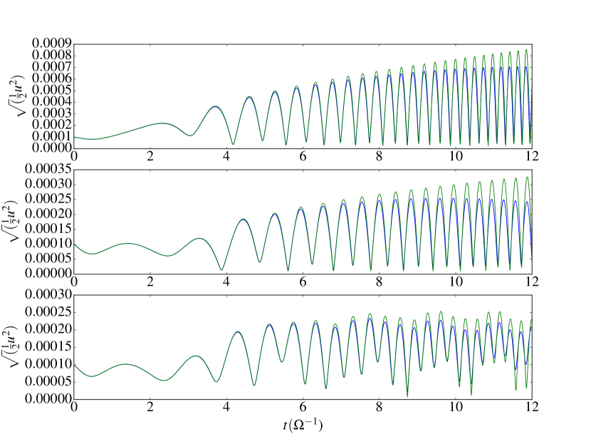
Figure 12: Rms velocity fluctuations of a shearing wave for a non-magnetized isothermal gas (top panel), ideal gas (center panel) and ideal+magnetized gas (bottom panel). The parameters are $Q=1.1368$, $\Sigma_{0}=1.0$, $\nu=0$, and $\eta=0$. Green curves represent the theoretical results while blue curves are those obtained with our self-gravity module. The resolution is 512 points per azimuthal wavelength.

We performed the same test for an initial $Q<1$, but complications arise in this configuration. Indeed, the code produces artificially very small leading perturbations at $t\simeq 0$ that are amplified exponentially when they move from leading to trailing (the ‘aliasing’ problem). As a result, the initial wave is mixed with artifical waves which can potentially grow faster. After a given time, the code fails to reproduce the theoretical solution. Note that filtering these leading modes gives the desired result.

References

- Armitage (2011) Armitage P. J., 2011, ARAA, 49, 195
- Armitage et al. (2001) Armitage P. J., Livio M., Pringle J. E., 2001, MNRAS, 324, 705
- Bai (2014) Bai X.-N., 2014, ApJ, 791, 137
- Balbus & Hawley (1991) Balbus S. A., Hawley J. F., 1991, ApJ, 376, 214
- Bareford & Hood (2015) Bareford M. R., Hood A. W., 2015, Philosophical Transactions of the Royal Society of London Series A, 373, 20140266
- Birn & Priest (2007) Birn J., Priest E. R., 2007, Reconnection of magnetic fields : magnetohydrodynamics and collisionless theory and observations
- Biskamp (1986) Biskamp D., 1986, Physics of Fluids, 29, 1520
- Boss (1997) Boss A. P., 1997, Science, 276, 1836
- Cameron (1978) Cameron A. G. W., 1978, Moon and Planets, 18, 5
- Cowley et al. (1997) Cowley S. C., Longcope D. W., Sudan R. N., 1997, Phys. Rep., 283, 227
- Evans et al. (2009) Evans II N. J., et al., 2009, ApJS, 181, 321
- Gammie (2001) Gammie C. F., 2001, ApJ, 553, 174
- Godard et al. (2009) Godard B., Falgarone E., Pineau Des Forêts G., 2009, AAp, 495, 847
- Goldreich & Lynden-Bell (1965) Goldreich P., Lynden-Bell D., 1965, MNRAS, 130, 125
- Hawley et al. (1995) Hawley J. F., Gammie C. F., Balbus S. A., 1995, ApJ, 440, 742
- Hillier et al. (2016) Hillier A., Takasao S., Nakamura N., 2016, preprint, (arXiv:1602.01112)
- Huang & Bhattacharjee (2013) Huang Y.-M., Bhattacharjee A., 2013, Physics of Plasmas, 20, 055702
- Kim & Ostriker (2001) Kim W.-T., Ostriker E. C., 2001, ApJ, 559, 70
- Kratter & Lodato (2016) Kratter K. M., Lodato G., 2016, preprint, (arXiv:1603.01280)
- Lee et al. (2003) Lee H., Ryu D., Kim J., Jones T. W., Balsara D., 2003, ApJ, 594, 627
- Lesur et al. (2014) Lesur G., Kunz M. W., Fromang S., 2014, AAp, 566, A56
- Loureiro & Uzdensky (2016) Loureiro N. F., Uzdensky D. A., 2016, Plasma Physics and Controlled Fusion, 58, 014021
- Loureiro et al. (2005) Loureiro N. F., Cowley S. C., Dorland W. D., Haines M. G., Schekochihin A. A., 2005, Physical Review Letters, 95, 235003
- Martin & Lubow (2011) Martin R. G., Lubow S. H., 2011, ApJ, 740, L6
- McNally et al. (2014) McNally C. P., Hubbard A., Yang C.-C., Mac Low M.-M., 2014, ApJ, 791, 62
- Mignone et al. (2007) Mignone A., Bodo G., Massaglia S., Matsakos T., Tesileanu O., Zanni C., Ferrari A., 2007, ApJs, 170, 228
- Paardekooper (2012) Paardekooper S.-J., 2012, MNRAS, 421, 3286
- Paczynski (1978) Paczynski B., 1978, ACTAA, 28, 91
- Park et al. (1984) Park W., Monticello D. A., White R. B., 1984, Physics of Fluids, 27, 137
- Parker (1972) Parker E. N., 1972, ApJ, 174, 499
- Petschek (1964) Petschek H. E., 1964, NASA Special Publication, 50, 425
- Priest & Forbes (1986) Priest E. R., Forbes T. G., 1986, JGR, 91, 5579
- Rafikov (2016) Rafikov R. R., 2016, preprint, (arXiv:1601.03009)
- Rice et al. (2014) Rice W. K. M., Paardekooper S.-J., Forgan D. H., Armitage P. J., 2014, MNRAS, 438, 1593
- Sarkar (1992) Sarkar S., 1992, Physics of Fluids, 4, 2674
- Sicilia-Aguilar et al. (2012) Sicilia-Aguilar A., et al., 2012, AAp, 544, A93
- Simon et al. (2013) Simon J. B., Bai X.-N., Armitage P. J., Stone J. M., Beckwith K., 2013, ApJ, 775, 73
- Simon et al. (2015) Simon J. B., Lesur G., Kunz M. W., Armitage P. J., 2015, MNRAS, 454, 1117
- Toomre (1964) Toomre A., 1964, ApJ, 139, 1217
- Ugai (1995) Ugai M., 1995, Physics of Plasmas, 2, 3320
- Zeman (1991) Zeman O., 1991, Physics of Fluids, 3, 951
- Zhu et al. (2010) Zhu Z., Hartmann L., Gammie C., 2010, ApJ, 713, 1143