Exercising Control When Confronted by a (Brownian) Spider

Abstract

We consider the Brownian “spider,” a construct introduced in Barlow et al. (1989) and in Dubins & Schwarz (1988). In this note, the author proves the “spider” bounds by using the dynamic programming strategy of guessing the optimal reward function and subsequently establishing its optimality by proving its excessiveness.

In memory of my mentor, Professor Larry Shepp (1936-2013)

1 Introduction

In this note, we consider the Brownian “spider,” a process also known as the “Walsh” Brownian motion, due to Barlow et al. (1989) and Dubins & Schwarz (1988). The Brownian spider is constructed as a set of $n\geq 1$ half-lines, or “ribs,” meeting at a common point, $O$. A Brownian motion on a spider starting at zero may be constructed from a standard reflecting Brownian motion ($|W_{t}|,t\geq 0$) by assigning an integer $i\in\{1,\ldots,n\}$ uniformly and independently to each excursion which is then transferred to an excursion on rib $i$ (here, $i$ should be interpreted as the index of the rib on which the next excursion occurs). It is helpful to think about the Brownian spider as a bivariate process; the first coordinate of the process is reflecting Brownian motion and the second coordinate of the process is the rib index. Formally, we define the Brownian spider process $Z_{t}$ as

$$Z_{t}=\left(|W_{t}|,R_{t}\right),t\geq 0$$ (1)

where $|W_{t}|$ is reflected Brownian motion and $R_{t}$ is the rib on which the process is located at time $t$. $|W_{t}|$ can be decomposed into excursions away from 0 with endpoints $t_{k}$ s.t. $|W_{t_{k}}|=0$. $R_{t}$ is constant between $t_{k}$ and $t_{k+1}$ for all $i$, and $R_{t}=i$ means the excursion occurs on the rib $i$. We define the supremum of reflected Brownian motion on each rib as

$$S_{i}(t)=\sup_{\{t:\,\,R_{t}=i\}}|W_{t}|,\,\,t\geq 0,\,i=1,...,n.$$

Below is a sample path realization of the Brownian spider for $n=3$. We use $W_{i}(t)$ to denote the process on the rib $i$:

$$W_{i}(t)=\left\{\begin{array}[]{cc}|W_{t}|&\text{ if }R_{t}=i\\ 0&\text{ if }R_{t}\neq i.\end{array}\right.$$ (2)

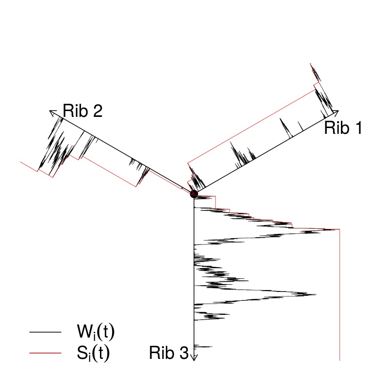
Figure 1: A sample path realization of the Brownian spider for $n=3$.

In an attempt to understand the unboundedness of Brownian motion on the spider up to time $t$, a natural question to ask is: what is $\mathbb{E}\left[\sum_{i=1}^{n}S_{i}(t)\right]$? However, Lester Dubins (personal communication with Larry Shepp) asked a different question. Dubins wished to design a stopping time to maximize the coverage of Brownian motion on the spider for a given expected time. That is, he wished to find

$$C_{n}:=\sup_{\{\tau:\,\,\mathbb{E}\left[\tau\right]=1\}}\mathbb{E}\left[S_{1}(\tau)+\ldots+S_{n}(\tau)\right],$$ (3)

where the supremum is calculated over all stopping times of mean one. Equivalently, Dubins wished to calculate the smallest $C=C_{n}$ such that for every stopping time $\tau$ the following inequality holds

$$\mathbb{E}\left[S_{1}(\tau)+S_{2}(\tau)+\ldots+S_{n}(\tau)\right]\leq C_{n}\sqrt{\mathbb{E}\left[\tau\right]}.$$ (4)

(note that for any stopping time $\tau$, $\mathbb{E}\left[S_{i}(\tau)\right]$ scales with with $\sqrt{\tau}$). The left side of equation (4) is the mean total measure of space visited on the spider up to time $\tau$.

For $n=0$, we, somewhat inconsistently, define $C_{0}$ in a similar way for ordinary Brownian motion without a reflecting barrier at zero. We seek the smallest constant $C_{0}$ for which the one-sided maximum satisfies

$$\mathbb{E}\left[\max_{\{0\leq t\leq\tau\}}W(\tau)\right]\leq C_{0}\sqrt{\mathbb{E}\left[\tau\right]}.$$ (5)

In this note, we will prove that the optimal bounds $C_{n}=\sqrt{n+1}$, for $n=0,1,2$. Without further delay, the author notes that the solution of the optimal bounds for $n=0,1,2$ is not new. The cases $n=0,1$ were solved by Dubins & Schwarz (1988), and the case $n=1$ was also independently solved by Gilat (1988) by a different method. The $n=2$ case was recently resolved by Dubins et al. (2009). What is new, however, is the dynamic programming strategy the author employs to find the bounds $C_{n}$ for $n=0,1,2$, which he believes to be the most tractable approach for solving for $C_{n}$ for all $n$ (despite much effort by many researchers, this problem remains open). The behavior of $C_{n}$ for large $n$ is interesting because when $n=\infty$, the total measure of space visited on the spider up to time $t>0$ is also infinite. This is because it is the total variation of a Brownian motion on $[0,t]$ because at each return to the node, a fresh rib is chosen.

Larry Shepp saw dynamic programming to be the root of all optimal control problems. In general, there are two strategies that can be used to solve a dynamic programming problem.

(A) Guess a candidate for an optimal strategy, calculate the reward function for the strategy, then prove its excessiveness.

(B) Guess the optimal reward function and establish its optimality by proving its excessiveness.

Unlike Dubins et al. (2009), which employs strategy (A), our approach is that of (B), and to the best of our knowledge, we are the first to do so. In stochastic optimization, strategy (B) reduces to “guessing” the right optimal control function. If one can guess the right function, the supermartingale becomes a martingale, and Itô calculus takes care of the rest. This approach appears prominently throughout Shepp’s most seminal works, specifically on p.634 of Shepp & Shiryaev (1993), on p.207 of Grigorescu et al. (2007), p.1528 of Shepp & Shiryaev (1996), on p.335 of Ernst et al. (2014), and most recently, on p.422 of Ernst & Shepp (2015).

The organization of this note is as follows: In Section 2, we formalize our guess for the optimal reward function. In Section 3, we establish the optimality of this function by proving its excessiveness, albeit only in the cases $n=0,1,2$. We conclude by arguing the viability of our strategy towards a solution of the general problem.

2 Our guess of the optimal reward function

Let $r=R_{0}$ be the index of the starting rib, $x$ be a fixed distance along the rib $r$, and $C$ and $M$ finite constants. In order to obtain the least upper bound $C_{n}$, we must solve a more general optimal stopping problem. Let $s_{1},s_{2},...,s_{n}\geq 0$ be the distances that have already been covered on each of the respective ribs at time $0$. For every value of $C>0$, and every choice of $r$ and $x$ such that $x\leq s_{r}$, and $s_{1},\ldots,s_{n}$, we must find the value of

$$V(x,r;s_{1},\ldots,s_{n};C):=\sup_{\{\tau:\,\,\mathbb{E}\left[\tau\right]\leq M\}}\mathbb{E}_{\{x,r,s_{1},\ldots,s_{n}\}}\left[S_{1}(\tau)+\ldots+S_{n}(\tau)-C\tau\right].$$ (6)

The subscript of the expectation, ${\{x,r,s_{1},\ldots,s_{n}\}}$, denotes that the process is currently at a distance $x$ on rib $r$ at time $0$. By abuse of notation, $S_{i}(\tau)$ denotes the furthest point covered on rib $i$ up to time $\tau$. Note that we must find $V(x,r;s_{1},\ldots,s_{n};C)$ not only for $x=0$ and $s_{1}=\ldots=s_{n}=0$, but for every point of the spider at $x$ on every rib $r$ as initial point, and every starting position for $s_{i},i=1,\ldots,n$.

In (6), the supremum is taken over bounded stopping times $\tau$. Even though we only need the case when the initial point is $O$ and when $s_{i}=0,\,\,i=1,\ldots,n$, standard martingale methods of solving optimal stopping problems do not work unless we can find the formula $V$ for every starting position (see, for example:  Brumelle (1971), Dynkin & Yushkevich (1979),  Dubins et al. (1994),  Rhee & Talagrand (1987), and  Walrand & Varaiya (1981)).

We “guess” that ${\hat{V}}(x,r,s_{1},\ldots,s_{n},C)$ should have the following properties:

(a) ${\hat{V}}(0,r,s_{1},\ldots,s_{n},C)$ does not depend on $r$ (if $x_{i}=0,r$ becomes irrelevant).

(b) $\frac{d}{dx}{\hat{V}}(x,r,s_{1},\ldots,s_{n},C)=0$ at $x=0$ $\forall r$.

(c) $\frac{d}{ds_{r}}{\hat{V}}(x,r,s_{1},\ldots,s_{n},C)=0$ at $x=s_{r}\,\,\forall\,r$.

(d) $\frac{1}{2}\frac{d^{2}}{dx^{2}}{\hat{V}}(x,r,s_{1},\ldots,s_{n},C)\leq C,\,0\leq x\leq s_{r},\,r=1,\ldots,n$.

(e) ${\hat{V}}(x,r,s_{1},\ldots,s_{n},C)\geq s_{1}+\ldots+s_{n}$, for all $0\leq x\leq s_{r}$ and $r=1,\ldots,n$.

(f) If strict inequality holds in property (e), $\frac{1}{2}\frac{d^{2}}{dx^{2}}{\hat{V}}(x,r,s_{1},\ldots,s_{n},C)=-C$, $0\leq x\leq s_{r}$.

Intuitively, at a stopping place, we are far from any boundary point where an $s$ would increase and thus we are willing to accept the reward ${\hat{V}}(x,r,s_{1},\ldots,s_{n},C)=s_{1}+\ldots+s_{n}$.

3 Establishing the optimality of the reward function

Theorem 3.1.

If we have a function ${\hat{V}}$ satisfying properties (a)-(f) in Section 2, then

$$V(x,r,s_{1},\dots,s_{n};C)\equiv{\hat{V}}(x,r,s_{1},\dots,s_{n},C).$$ (7)

Proof.

Consider the process

$$Y(t)={\hat{V}}\left(Z_{t},{\bf S}(t),C\right)-Ct,\,\,\,t\geq 0$$ (8)

where $\mathbf{S}(t)=\left(S_{1}(t),...,S_{n}(t)\right)$. $Y(t)$ is a continuous local supermartingale at $x=0$ by properties (a) and (b), at $x=s_{r}$ by property (c), and at any $x$ by property (d). For any bounded stopping time $\tau$, it follows from the optional sampling theorem that $\mathbb{E}\left[Y(\tau)\right]\leq Y(0)$. Property (e) gives us that for any bounded $\tau$,

$$\mathbb{E}_{\{x,r,s_{1},\ldots,s_{n}\}}\left[S_{1}(\tau)+\ldots+S_{n}(\tau)-C\tau\right]\leq{\hat{V}}\left(x,r,s_{1},\ldots,s_{n},C\right).$$ (9)

From the definition of $V$ in (6), we must have $V\leq\hat{V}$.

We now consider the reverse inequality $V\geq{\hat{V}}$. By property (f), equality holds in the last argument for the “right $\tau$.” Although this “right $\tau$” does not always exist in such problems, it does for our problem; the “right $\tau$” is the first entry time of the underlying Markov process $(Z,S)$ in the set where equality holds in (e). Further, this “right $\tau$” is a particular stopping time that is “approximable by uniformly bounded ones.” Larry Shepp used the phrase “approximable by uniformly bounded ones” to denote that we can take the “right $\tau$” at which the equality is attained, approximate this “right $\tau$” with “right $\tau$” $\wedge\,\,n$ for $n\geq 1$, and then proceed to pass to the limit for $n$. This is valid in our setting since the “right $\tau$” has finite expectation. When property (f) holds, and when equality holds in (d), $Y$ will be a local martingale up to the first entry of the underlying Markov process $(Z,S)$ into the the set where equality holds in (e). Since the “right $\tau$” has a finite expectation, we may invoke the standard form of Doob’s stopping theorem for bounded stopping times, as in Shiryaev (1978). Thus,

$$\mathbb{E}_{\{x,r,s_{1},\ldots,s_{n}\}}\left[S_{1}(\tau)+\ldots+S_{n}(\tau)-C\tau\right]\geq{\hat{V}}\left(x,r,s_{1},\ldots,s_{n},C\right).$$ (10)

and one can optimize over $\tau$ on both sides. The reverse inequality $V\geq{\hat{V}}$ thus holds and thus $V\equiv{\hat{V}}$, completing the proof.

∎

If we can find the right ${\hat{V}}$ satisfying properties (a)-(f), we then know that

$$A_{n}(C):=V\left(O,r,0,\ldots,0;C\right)=\frac{\theta_{n}}{C},$$ (11)

where $\theta_{n}$ is a number independent of $C$. $V$ must be of the form $\frac{\theta_{n}}{C}$ because a scaling argument allows us to reduce the problem to any one value of $C$. This is because we will show that

$$V\left(x,r,s_{1},\ldots,s_{n};C\right)=\frac{1}{C}V\left(Cx,r,Cs_{1},\ldots,Cs_{n};1\right).$$ (12)

Note that if we start at $x=O$ and $s_{1}=\ldots=0$ then above form for $A_{n}(C)$ is obtained. Let

$$S(\tau)\triangleq S_{1}(\tau)+...+S_{n}(\tau).$$

For any $C$ and any $\tau$, $\mathbb{E}\left[S(\tau)\right]\leq A_{n}(C)+C\mathbb{E}\left[\tau\right]$. If we specify $m=\mathbb{E}\left[\tau\right]$ for any fixed stopping time $\tau$, then we will obtain the best upper bound by minimizing over $C$, which is

$$\mathbb{E}\left[S(\tau)\right]\leq\inf\left(\frac{\theta}{C}+Cm\right).$$

The infimum is attained at $C=\sqrt{\frac{\theta_{n}}{m}}$ and gives the bound $C_{n}=2\sqrt{\theta_{n}}$ for any $n$. Thus we need only find $V(O;C)$ for any one value of $C$.

3.1 Solution for n=0,1,2

Corollary 3.2.

$C_{0}=1$.

Proof.

For $n=0$, consider the function

$${\hat{V}}\left(x,s,C\right)=C\left(\left(x-s+\frac{1}{2C}\right)^{+}\right)^{2}+s.$$

We note that properties (a)-(f) hold, and so for $x=s=0$, and for any $C>0$

$$\mathbb{E}\left[S_{\tau}\right]\leq C\mathbb{E}\left[\tau\right]+\frac{1}{4C}.$$ (13)

Minimizing over $C$, i.e., taking $C=\frac{1}{2\sqrt{\mathbb{E}\left[\tau\right]}}$, as above for any $\tau$, we obtain the inequality

$$\mathbb{E}\left[S(\tau)\right]\leq\sqrt{\mathbb{E}\left[\tau\right]}$$ (14)

for all $\tau$, i.e., $C_{0}=1$. ∎

Corollary 3.3.

$C_{1}=\sqrt{2}$.

Proof.

For $n=1$, the right ${\hat{V}}$ is given by:

$${\hat{V}}\left(x,s,C\right)=Cx^{2}+\frac{1}{2C},\quad 0\leq x\leq s\leq\frac{1}{2C};$$ (15)

$${\hat{V}}\left(x,s,C\right)=C\left(\left(x-s+\frac{1}{2C}\right)^{+}\right)^{2}+s,\quad 0\leq x\leq s,\,\,s>\frac{1}{2C}.$$

We use the above argument to see that $A_{2}(C)=\frac{1}{2C}$ and $\theta_{1}=\frac{1}{2}$ and so $C_{1}=\sqrt{2}$. ∎

Corollary 3.4.

$C_{2}=\sqrt{3}$.

Proof.

For $n=2$, ${\hat{V}}$ is, for $i\neq j$ and $s_{1}+s_{2}\leq\frac{1}{C}$,

$${\hat{V}}(x,r,s_{1},s_{2},C)=Cx^{2}-Cx(s_{i}-s_{j})+\frac{C(s_{1}^{2}+s_{2}^{2})}{2}+\frac{3}{4C},\quad 0\leq x\leq s_{i}.$$ (16)

We further simplify equation (16) as follows:

$${\hat{V}}(x,r,s_{1},s_{2},C)=C\left(\left(x-\left(s_{i}-\frac{1}{2C}\right)\right)^{+}\right)^{2}+C\left(\left(-x-\left(s_{j}-\frac{1}{2C}\right)\right)^{+}\right)^{2}+s_{1}+s_{2},$$ (17)

where $0\leq x\leq s_{i},s_{1}+s_{2}\geq\frac{1}{C}$. We can use the above argument to see that with $V(O;C)=\frac{3}{4C}$ we arrive at $C_{2}=\sqrt{3}$. ∎

4 $n=3$ and beyond

At present, we possess a non-trivial but ultimately incomplete strategy for addressing the case $n=3$. Our strategy is to develop the “correct” nonlinear Fredholm equation in order that we may reduce the problem to that of a nonlinear integral recurrence. Based on simulation approaches, we conjecture the following about the constant:

Conjecture 4.1.

The $\sqrt{n+1}$ pattern for the spider constant does not hold for $n=3$.

Further, it is likely that the spider constant for $n=3$ is not an elementary number.

5 Final Remarks

We are hopeful of a solution to the general $n$ case for the Dubins spider and maintain that our proposed dynamic programming approach constitutes the most tractable direction for solving the problem, for the following reasons: 1) The use of linear programming would be infeasible because the approximate linear programming would be large and unwieldy, making accurate numerics impossible. 2) Bellman’s dynamic programming method seems intractable for the same reason as that of using linear programming. 3) The more standard method of dynamic programming, namely that of guessing a candidate for an optimal strategy, calculating the reward function of the strategy, and proving its excessiveness (as most recently done by Dubins et al. (2009)) was unsuccessful in obtaining the general solution.

References

- Barlow et al. [1989] Barlow, M., Pitman, J., & Yor, M. (1989). On Walsh’s Brownian motions. In Séminaire de probabilités de Strasbourg (pp. 275–293). volume 1372.
- Brumelle [1971] Brumelle, S. (1971). Some inequalities for parallel-server queues. Operations Research, 19, 402–413.
- Dubins et al. [2009] Dubins, L., Gilat, D., & Meilijson, I. (2009). On the expected diameter of an bounded martingale. The Annals of Probability, 37, 393–402.
- Dubins & Schwarz [1988] Dubins, L., & Schwarz, G. (1988). A sharp inequality for submartingales and stopping times. Astérisque, 157, 129–145.
- Dubins et al. [1994] Dubins, L., Shepp, L., & Shiryaev, A. (1994). On optimal stopping rules and maximal inequalities for Bessel processes. Theory of Probability and Applications, 38, 226–261.
- Dynkin & Yushkevich [1979] Dynkin, E., & Yushkevich, A. (1979). Controlled Markov Processes. Springer.
- Ernst et al. [2014] Ernst, P., Foster, D., & Shepp, L. (2014). On optimal retirement. Journal of Applied Probability, 51, 333–345.
- Ernst & Shepp [2015] Ernst, P., & Shepp, L. (2015). Revisiting a theorem of L.A. Shepp on optimal stopping. Communications on Stochastic Analysis, 9, 419–423.
- Gilat [1988] Gilat, D. (1988). On the ratio of the expected maximum of a martingale and the norm of its last term. Israel Journal of Mathematics, 63, 270–280.
- Grigorescu et al. [2007] Grigorescu, I., Chen, R., & Shepp, L. (2007). Optimal strategy for the Vardi casino with interest payments. Journal of Applied Probability, 44, 199–211.
- Rhee & Talagrand [1987] Rhee, W., & Talagrand, M. (1987). Martingale inequalities and NP-complete problems. Mathematics of Operations Research, 12, 177–181.
- Shepp & Shiryaev [1993] Shepp, L., & Shiryaev, A. (1993). The Russian option: reduced regret. Annals of Applied Probability, 3, 631–640.
- Shepp & Shiryaev [1996] Shepp, L., & Shiryaev, A. (1996). Hiring and firing optimally in a large corporation. Journal of Economic Dynamics and Control, 20, 1523–1539.
- Shiryaev [1978] Shiryaev, A. (1978). Optimal Stopping Rules. Springer-Verlag.
- Walrand & Varaiya [1981] Walrand, J., & Varaiya, P. (1981). Flows in queueing networks: a martingale approach. Mathematics of Operations Research, 6, 387–404.