Scaling solutions for Dilaton Quantum Gravity

Abstract

Scaling solutions for the effective action in dilaton quantum gravity are investigated within the functional renormalization group approach. We find numerical solutions that connect ultraviolet and infrared fixed points as the ratio between scalar field and renormalization scale $k$ is varied. In the Einstein frame the quantum effective action corresponding to the scaling solutions becomes independent of $k$.

The field equations derived from this effective action can be used directly for cosmology. Scale symmetry is spontaneously broken by a non-vanishing cosmological value of the scalar field. For the cosmology corresponding to our scaling solutions, inflation arises naturally. The effective cosmological constant becomes dynamical and vanishes asymptotically as time goes to infinity.

I Introduction

There is accumulating evidence that quantum gravity may be non-perturbatively renormalizable due to the existence of an ultraviolet fixed point. This scenario of asymptotic safety weinberg1979ultraviolet has been found in four-dimensional renormalization group investigations Reuter:1996cp , based on functional renormalization for the effective average action Wetterich:1992yh ; Reuter:1993kw . Many extensions of the truncation beyond the simplest Einstein-Hilbert truncation have confirmed the presence of the ultraviolet fixed point Dou:1997fg ; Souma:1999at ; Reuter:2001ag ; Litim:2003vp ; Codello:2006in ; Machado:2007ea ; Codello:2008vh ; Fischer:2006fz ; Benedetti:2009rx ; Eichhorn:2010tb ; Manrique:2010am ; Donkin:2012ud ; Christiansen:2012rx ; Rechenberger:2012dt ; Dietz:2012ic ; Codello:2013fpa ; Falls:2013bv ; Benedetti:2013jk ; Christiansen:2014raa ; Christiansen:2015rva ; Dietz:2015owa ; Demmel:2015oqa ; Falls:2015qga ; Gies:2015tca ; Gies:2016con , for reviews see Niedermaier:2006wt ; Percacci:2007sz ; Litim:2011cp ; Reuter:2012id ; Nagy:2012ef . Similar ideas have been explored in other quantum field theories, see, e.g., Gies:2009hq ; Braun:2010tt ; Litim:2014uca . Interactions with matter have been included Dou:1997fg ; Folkerts:2011jz ; Harst:2011zx ; Dona:2013qba ; Oda:2015sma ; Meibohm:2015twa ; Eichhorn:2016esv , with emphasis on scalar matter in refs. Narain:2009fy ; Narain:2009gb ; Percacci:2015wwa ; Dona:2015tnf ; Labus:2015ska . Additional arguments in favor of asymptotic safety arise from different approaches to quantum gravity Hamber:2009mt ; Ambjorn:2009ts .

In the presence of an ultraviolet fixed point the flow of couplings can be extended to the limit where the renormalization scale $k$ goes to infinity. Within functional renormalization, observable quantities are obtained in the opposite limit $k\to 0$. Furthermore, the gravitational quantum field equations relevant for cosmology arise for $k\to 0$. It is therefore important to find smooth trajectories from the ultraviolet to the infrared limit as $k$ decreases to zero Donkin:2012ud ; Christiansen:2012rx ; Nagy:2012rn .

Gravity coupled to a scalar field offers the interesting perspective that a realistic scale-symmetric theory of gravity and particle physics can be formulated if the Planck mass is given by a scalar field $\chi$ Fujii:1982ms ; Wetterich:1987fm ; Shaposhnikov:2008xi . In the absence of explicit mass scales the scale $k$ can only be compared to $\chi$, with IR-limit $k/\chi\to 0$. If cosmological solutions for $\chi$ approach an infrared fixed point with exact scale symmetry the “dilatation anomaly” close to the fixed point can give rise to dynamical dark energy or quintessence Wetterich:1987fm . The crossover between an ultraviolet and infrared fixed point can connect inflation and present dynamical dark energy, both described by the same cosmon field Wetterich:2014gaa . Realistic cosmology is found in a picture where the universe is not expanding during radiation and matter domination Wetterich:2013aca and the big bang singularity is absent Wetterich:2014zta .

In the functional renormalization group approach to quantum gravity the system of a scalar field coupled to gravity was first studied in ref. Narain:2009gb ; Narain:2009fy . The existence of a “global scaling solution” for all $k$ and $\chi$, with general scalar potential and scalar-field dependent coefficient of the curvature scalar, was investigated in ref. Henz:2013oxa . Recent advances towards a global scaling solution have been made in Percacci:2015wwa ; Borchardt:2015rxa .

In the present work we derive for the first time candidates for global scaling solutions in dilaton gravity. These solutions are obtained from a qualitatively improved approximation to the effective action in comparison to those used in previous works: Firstly, we include a $\chi$-dependent coefficient of the scalar kinetic term, called the kinetial. This closes a systematic derivative expansion in the second order of derivatives. The second necessary improvement concerns the computation of dynamical correlation functions on the basis of the expansion scheme put forward in refs. Christiansen:2012rx ; Christiansen:2014raa ; Christiansen:2015rva , for gravity-matter systems see refs. Meibohm:2015twa ; Meibohm:2016mkp ; Eichhorn:2016esv . This goes beyond the standard background field approximation. With its relation to the constraints of diffeomorphism symmetry in a gauge-fixed setting it is at the root of background independence, for discussions see e.g. ref. Litim:2002ce ; Folkerts:2011jz ; Christiansen:2015rva ; Meibohm:2015twa . The expansion around a flat background as well as a vertex construction allow us to compute the running of the kinetial as well as to disentangle fluctuating and background fields.

II Setup

We aim at finding global fixed point solutions for the effective action of dilaton gravity

$$\Gamma=\int_{x}\sqrt{g}\left(V(\chi^{2})-\frac{1}{2}F(\chi^{2})\,R+\frac{1}{2}K(\chi^{2})g^{\mu\nu}\partial_{\mu}\chi\partial_{\nu}\chi\right)\,,$$ (1)

where $\int_{x}=\int d^{4}x$. The three functions $V$, $F$ and $K$ depend on a scalar field $\chi$ and the renormalization scale $k$. For a scaling solution, the dimensionless functions $V/k^{4}$, $F/k^{2}$ and $K$ only depend on the dimensionless ratio $y=\chi^{2}/k^{2}$. For fixed $k=\mu$ the effective action (1) constitutes a model of variable gravity, for which the cosmology is discussed in detail in Wetterich:2013jsa . In this work we extract the scale dependence of the functions $V$, $F$ and $K$ from the functional renormalization group. This translates directly to the $\chi$-dependence of these functions and therefore to the field equations relevant for cosmology. We work with dimensionless functions and fields.

To derive the flow equations, we consider $\Gamma[\bar{g},\bar{\chi};g,\chi]$. Here, $\bar{g}$, $\bar{\chi}$ are background fields and $h=g-\bar{g}$, $\delta\chi=\chi-\bar{\chi}$ are the dynamical fluctuation fields. While the occurrence of the background metric is inherent to any gauge-fixed approach to quantum gravity, the dependence on the dilaton background field is only introduced via the regulator term, see refs. Litim:2002hj ; Dietz:2015owa . The identification $\bar{g}=g$, $\bar{\chi}=\chi$ eliminates generalized gauge fixing terms and results in the gauge invariant effective action $\Gamma[g,\chi]$. We are interested in the scaling solution for $\Gamma[g,\chi]$. The flows of $V$, $F$ and $K$ are extracted from the flow of the two point functions for the fluctuating fields $h$ and $\delta\chi$ Christiansen:2014raa ; Christiansen:2015rva . We work in deDonder gauge and neglect the ghost contributions, as they do not couple directly to the dilaton field, as well as some subleading terms in the $k$-dependence of the regulator. We perform a systematic expansion in powers of $h$ to disentangle contributions from background and fluctuating fields. Accordingly, we compute the flow equations for $V$ and $F$ via the momentum independent and dependent part of the flow of the transverse-traceless graviton $2$-point function, respectively. Moreover, we use the momentum-dependent part of the scalar $2$-point function for the flow of $K$, expanding around flat space Christiansen:2014raa . The full equations are too long to be displayed here.

III Large field limit

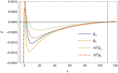
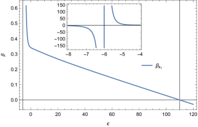
Figure 1: Flowing couplings. The $\beta$-functions $v_{0},f_{0},v_{1},f_{1},k_{1}$ are shown as functions of $\epsilon$, with other couplings kept fixed at values given by eq. (9). The simultaneous zero at $\epsilon=\epsilon_{0}=109.97$, as well as the pole at $\epsilon=-6$ are clearly visible.

We first consider large $y$, which for finite field $\chi$ is equivalent to sending the renormalization scale $k\to 0$ and thus constitutes the infrared limit of dilaton gravity. For fixed $k$ this is the limit $\chi\to\infty$. One possible IR-limit implies weak gravity with $F\sim y$. For $\chi\to\infty$ the effective gravitational constant goes to zero and the gravitational degrees of freedom decouple. Furthermore, if $K$ and $V/k^{4}$ approach constants the asymptotic behavior in the scalar sector is a free theory. This type of IR fixed point has a very simple physical content: a free massless scalar and a free graviton, with vanishing gravitational coupling. We investigate the scaling solutions connected to this fixed point.

For finite $y$ we expand $V$, $F$ and $K$ in inverse powers of $y$. For a free scalar field with $F=\xi y$ and $K=K_{0}$, a rescaling of $\chi$ multiplies $\xi$ and $K_{0}$ with the same factor. In consequence, only the ratio $\epsilon=K_{0}/\xi$ appears in the flow equations. More explicitly, for large $y$ we make the ansatz

$$V =\sum_{j=0}^{a}\frac{v_{j}y^{-j}}{j!\xi^{j}}\,,\qquad F=\xi y+\sum_{j=0}^{b}\frac{f_{j}y^{-j}}{j!\xi^{j}},\,$$

$$K =\xi\epsilon+\sum_{j=1}^{c}\frac{k_{j}y^{-j}}{j!\xi^{j-1}}\,.$$ (2)

Switching to $x=1/(\xi y)$ and evaluating the flow at fixed $x$, one finds to first order in powers of $x$ the set of flow equations

$$\partial_{t}V =-4V-2x\frac{\partial V}{\partial x}+\frac{A_{V}}{B^{3}}+\frac{C_{V}}{B^{4}}x\,,$$

$$\partial_{t}F =-2F-2x\frac{\partial F}{\partial x}+\frac{A_{F}}{B^{3}}+\frac{C_{F}}{B^{4}}x\,,$$

$$\partial_{t}K =-2x\frac{\partial K}{\partial x}+\frac{C_{K}}{B^{4}}x\,,$$ (3)

with $\partial_{t}=k\partial_{k}$ and

$$B=\epsilon+6=\frac{K_{0}}{\xi}+6.$$ (4)

The terms $-4V$ and $-2F$ reflect the dimensionality of $V$ and $F$, while the terms $-2x\partial V/\partial x$, $-2x\partial F/\partial x$ and $-2x\partial K/\partial x$ result from translating the flow to fixed $x$. The coefficients $A_{i}$ and $C_{i}$ are computed from the one loop form of the flow equation for the effective action. They read

$$A_{V}= \frac{1}{192\pi^{2}}\left(9\epsilon^{3}+82\epsilon^{2}+612\epsilon+2760\right)\,,$$ (5)

$$C_{V}= \frac{1}{2592\pi^{2}}\left(1080f_{0}\epsilon^{3}-3240f_{0}\epsilon^{2}-62208f_{0}\epsilon\right.$$

$$\left.+1080k_{1}\epsilon^{2}-3240k_{1}\epsilon-62208k_{1}+383v_{0}\epsilon^{4}\right.$$

$$\left.+5004v_{0}\epsilon^{3}+51120v_{0}\epsilon^{2}+278208v_{0}\epsilon+382320v_{0}\right),$$

$$A_{F}= \frac{1}{3456\pi^{2}}\left(-253\epsilon^{3}-6094\epsilon^{2}-36240\epsilon-51840\right),$$

$$C_{F}= \frac{1}{5184\pi^{2}}\left(2148f_{0}\epsilon^{3}-2916f_{0}\epsilon^{2}-98712f_{0}\epsilon+\right.$$

$$\left.2310k_{1}\epsilon^{2}-972k_{1}\epsilon-92880k_{1}-345v_{0}\epsilon^{4}\right.$$

$$\left.-23498v_{0}\epsilon^{3}-213492v_{0}\epsilon^{2}-546552v_{0}\epsilon\right.$$

$$\left.-263520v_{0}\right)\,,$$

$$C_{K}= \frac{1}{36\pi^{2}}\left(-\epsilon^{4}+90\epsilon^{3}+2079\epsilon^{2}+12636\epsilon+26244\right)\,.$$

The fluctuation contributions do not enter the flow of the leading terms $F=\xi/x$ and $K=K_{0}$ such that $\xi$ and $K_{0}$, and therefore also $\epsilon$, are arbitrary couplings or “integration constants”. The appearance of a free parameter $\epsilon$ corresponds to the undetermined $\xi$ in an earlier calculation Henz:2013oxa with field independent $K=K_{0}=1$.

We are interested in fixed point solutions where the left hand side of (3) vanishes. The resulting system of differential equations for the $x$-dependence is closed in every order in the expansion in $x$. The fixed points for the $x$-independent terms depend on $\epsilon$ and are given by

$$v_{0}=\frac{A_{V}}{4B^{3}}\,,\qquad\ f_{0}=\frac{A_{F}}{2B^{3}}\,.$$ (6)

Similarly, one has $k_{1}=C_{K}/(2B^{4})$. Inserting these values in $C_{V}$ and $C_{F}$ yields $v_{1}$ and $f_{1}$.

An interesting particular solution arises when one chooses integration constants such that $C_{K}=0$. This resembles the system investigated in Henz:2013oxa . The condition $C_{k}=0$ fixes $\epsilon$ to a certain $\epsilon_{0}$. For this value the fixed point solution is given by

$$\begin{array}[]{l@{\quad}l@{\quad}l}v_{0}=1.10\cdot 10^{-3},&f_{0}=-3.89\cdot 10^{-3},&\epsilon_{0}=109.97,\\[8.61108pt] v_{1}=2.32\cdot 10^{-6},&f_{1}=-2.81\cdot 10^{-6},&k_{1}=0.\end{array}$$ (9)

It is the only real solution of this type which obeys the stability condition $\epsilon\geq-6$.

The $\beta$-functions for the couplings $v_{0},v_{1},f_{0},f_{1},k_{1}$ correspond to the coefficients in the expansion of the r.h.s. of eq. (3) in powers of $x$, with eq. (2) inserted. The $\beta$-functions depend on the couplings. We plot them in figure 1 for $v_{0},f_{0},v_{1},f_{1}$and $k_{1}$ given by eq. (9), as a function of $\epsilon$ which is left free. They show a simultaneous zero at $\epsilon_{0}=109.97$ as well as the pole at $\epsilon=-6.$ We point out that our approximation is no longer valid for $B\to 0$.

IV Global solution

The expansion (2) can be extended to rather high powers of $x$, and one may perform Padé approximations similar to ref. Henz:2013oxa . It is clear that such expansions will become unreliable for small $\chi/k$ or large $x$, which we identify with the ultraviolet limit. In order to connect with the region of large $x$ or small $y$ we need the full flow equations for the dimensionless functions $V/k^{4}$, $F/k^{2}$ and $K$. For simplicity, we keep the notation $\{V,F,K\}$ for the dimensionless quantities. The system of flow equations has been computed using algebraic algorithms. We have been able to solve numerically the fixed point equations $\partial_{t}V=\partial_{t}F=\partial_{t}K=0$ for the full functions $V(y),\ F(y)$ and $K(y)$, except for a range of very small $y$. Initial conditions for the numerical solution are chosen at large $y$, where the expansion (2) is valid and can be solved analytically. More precisely, we have taken the expansion (2) for $a=b=c=5$ and $y_{\text{in}}=10^{5}$. In figure 2 we display the numerical solutions for $\epsilon=\epsilon_{0}$ given by eq. (9). Note that there is no point at which $\frac{1}{2}F-V\approx 0$, meaning that the previously bothersome singularity discussed in ref. Percacci:2015wwa is not approached by the global scaling solution.

We have also investigated solutions with values of $\epsilon$ different from $\epsilon_{0}$. We were only able to obtain global solutions in the vicinity of $\epsilon_{0}$, and only for a finite set of values for $\epsilon$. While $V$ and $F$ are largely independent of $\epsilon$, $K$ is rescaled by $\epsilon$ for large $y$, while $\epsilon$ becomes less and less important for $y\to 0$.

For an estimate of the numerical error we compute the values of the $\beta$-functions for our numerical solution, which should be zero. They are normalized to the internal accuracy of the implicit numerical differential equation solver employed, which was set to $8$ decimal digits. As long as this relative error is smaller than $1$, we can assume the error to be negligible. This is the case for most parts of the interval under consideration, with only small, local deviations due to interpolation errors between the grid points of the numerical solution. These are inevitable when taking derivatives to compute the $\beta$-functions from the numerical solutions.

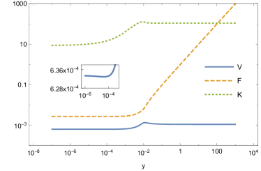
Figure 2: Global numerical solution for the functions $V(y)$, $F(y)$ and $K(y)$ in a double-log plot. The matching with the Taylor expansion was carried out at $y=10^{5}$.

V small field limit

For an investigation of the UV-behavior for $\chi/k\to 0$ we first consider the truncation where $V$, $F$ and $K$ are $\chi$-independent. A scaling solution with these properties closely resembles pure gravity in the Einstein-Hilbert truncation Reuter:1996cp , except for the presence of a massless scalar field. In this approximation the coupling between the scalar and the metric arises purely from the kinetic term. We include the possibility of a $k$-dependent wave function renormalization $Z$, or anomalous dimension $\eta=-\partial\log Z/\partial\log k$. The wave function renormalization is defined by $Z=K(y=0)$. At fixed $y_{R}=Zy$ only the anomalous dimension $\eta$ (and not $Z$) appears in the flow equations. Here, $\eta$ is determined by requiring that the $\eta$-dependent $\beta$-functions maintain for $K(y_{R}=0)$ an arbitrary $k$-independent value. The solution

$$V=0.0006460\,,\quad F=0.002757\,,\quad\eta=1.6669\,,$$ (10)

can be interpreted as the Einstein-Hilbert approximation to our system. It provides further evidence for the validity of the Asymptotic Safety Scenario in a truncation extended by a running kinetial.

In figure 2 we have only plotted the range $y>10^{-7}$ for our numerical solution. For very small $y$ the numerics become unstable. This is due to non-analytic behavior which leads to diverging derivatives and therefore numerical instabilities. Investigating the first derivative of the numerical solutions, we find that they diverge as $y^{-\alpha}$ with $\alpha=\frac{1}{2}$ for $y\to 0$. This explains why previous attempts Narain:2009fy , Percacci:2015wwa , Henz:2013oxa to expand in integer powers of $y$ were not well suited. A best fit for the three functions in the limit $y\to 0$, based on data generated from the numerical solutions for $10^{-7}\leq y\leq 10^{-5}$, is given by

$$V(y)= 6.3350\cdot 10^{-4}-1.7137\cdot 10^{-4}\,y^{1/2}$$

$$+8.3172\cdot 10^{-3}\,y+0.5626\,y^{3/2}\,,$$

$$F(y)= 2.7077\cdot 10^{-3}-3.7688\cdot 10^{-4}\,y^{1/2}$$

$$+3.6550\cdot 10^{-3}\,y+2.4944\,y^{3/2}\,,$$

$$K(y)= 8.7018+455.269\,y^{1/2}$$

$$+12940.3\,y+223285\,y^{3/2}\,.$$ (11)

We observe that the constants approached by $V$ and $F$ in the limit $y\to 0$ are very close to the Einstein-Hilbert truncation (10). This is no coincidence: For small $y$ our system approaches the UV fixed point of asymptotically safe quantum gravity. The slight numerical differences for $V(0)$ and $F(0)$ may arise from the small $y$-dependence of $V$, $F$ and $K$ in equation (11), which has been neglected in the truncation leading to the values (10). This may have a stronger influence on the correct behavior of $K(y\to 0)$ and on the value of the anomalous dimension. Extrapolating eq. (11) to $y\to 0$ would imply $\eta=0$. On the other hand, it is not excluded that the correct matching of the proposed scaling solution with the behavior for $y\to 0$ leads to constraints on the allowed values of $\epsilon$. We are mainly interested here in the generic IR-behavior which does not depend on the precise details of the extreme limit $y\to 0$.

VI Conformal invariants

Conformal or Weyl transformations of the metric, $g_{\mu\nu}=\omega^{2}(\chi)\tilde{g}_{\mu\nu}$, map the set of functions $\{V,F,K\}$ to a new set $\{\tilde{V},\tilde{F},\tilde{K}\}$. By virtue of field relativity the physical content of a model is specified by the two invariants under this rescaling, namely Wetterich:2015ccd

$$\hat{V}=\frac{V}{F^{2}},\qquad\hat{K}=\frac{K}{F}+\frac{6y}{F^{2}}\left(\frac{\partial F}{\partial y}\right)^{2}\,.$$ (12)

In figure 3 we show these invariants for the numerical solutions with different values of $\epsilon$. While $\hat{V}$ shows very little $\epsilon$ dependency, the scaling $\hat{K}\sim\epsilon$ is realized only for large $y$. The solutions with different $\epsilon$ seem not to be equivalent.

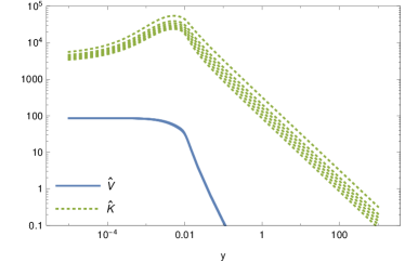
Figure 3: Invariants $\hat{V}$ and $\hat{K}$ for the fixed point solution for different values of $\epsilon$ in the vicinity of $\epsilon_{0}$.

The invariants obey

$$\lim_{y\to\infty}\hat{V}=0\,,\qquad\qquad\lim_{y\to\infty}\hat{K}=0.$$ (13)

As both $V$ and $K$ go to a constant for $y\to\infty$, while $F$ grows with $\xi y$, we can immediately understand that the ratios $V/F^{2}$ and $K/F$ vanish in this limit. Furthermore, we have $y(\partial F/\partial y)^{2}/F^{2}=1/y$. The potential $\hat{V}$ exhibits a maximum located at

$$y_{\text{max}}=0.02\,,\qquad\qquad\hat{V}(y_{\text{max}})=87\,.$$ (14)

The vanishing of $\hat{V}$ for $y\to\infty$ implies that the effective cosmological constant goes to zero asymptotically for cosmological solutions where $\chi(t\to\infty)\to\infty$ Wetterich:1987fm .

VII Effective action in the Einstein frame

Physical features of our system are most readily visible in the Einstein frame, which is reached by a Weyl scaling leading to $\tilde{F}=M^{2}/k^{2}$. Further using a rescaling of the scalar field to bring the kinetic term to standard form yields in the Einstein frame the effective action

$$\Gamma=\int_{x}\sqrt{g}\left(M^{4}\hat{V}(\phi)-\frac{1}{2}M^{2}\,R+\frac{1}{2}g^{\mu\nu}\partial_{\mu}\phi\partial_{\nu}\phi\right)\,.$$ (15)

From the kinetic term

$$\frac{M^{2}\hat{K}}{2k^{2}}\partial^{\mu}\chi\partial_{\mu}\chi=\frac{1}{2}\partial^{\mu}\phi\partial_{\mu}\phi\,,\quad\quad\hat{K}=\frac{16}{\alpha^{2}y}\,,$$ (16)

one infers for constant $\alpha$

$$\frac{1}{y^{2}}=\exp\left(-\frac{\alpha\phi}{M}\right),\quad V=M^{4}\hat{V}=\frac{v_{0}M^{4}}{\xi^{2}}\exp\left(-\frac{\alpha\phi}{M}\right),$$ (17)

with modifications if $\alpha$ depends on $y$. We observe that $y$ is a function of $\phi/M$, not involving $k$. All memory of $k$ has disappeared in the Einstein frame. In figure 4 we plot the dimensionless potential in the Einstein frame $V/M^{4}=\hat{V}$ as a function of $\tilde{\phi}=\phi/M$. For the values of $\epsilon$ for which numerical solutions could be established the potential has a maximum for small values of $\tilde{\phi}$, as shown in the inset.

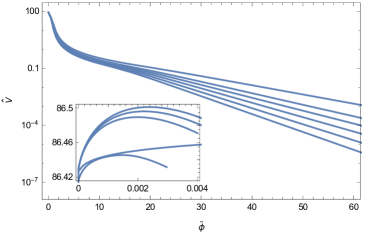
Figure 4: Scalar potential $V/M^{4}$ in the Einstein frame for a standard normalization of the scalar field. We show $\hat{V}$ as a function of $\tilde{\phi}=\phi/M$ for different values of $\epsilon$ around $\epsilon_{0}$. Note the maximum for small $\tilde{\phi}$ as well as the exponential tail for large $\tilde{\phi}$.

VIII Discussion

In this note we present for the first time candidates for a global scaling solution for dilaton quantum gravity. We find several striking features:

(i) For the scaling solution the effective action in the Einstein frame shows no dependence on $k$. A realistic form of gravity results directly for the scaling solution, without the need to deviate from the fixed point. Variation of the effective action (15) yields the quantum field equations and one may discuss cosmological solutions. For fixed $\chi$ the limit $k\to 0$ corresponds to $\phi\to\infty$, but for arbitrarily small $k$ we can always find values of $\chi$ such that $\phi$ is finite. We may also consider the possibility that a separate physical cutoff sale $\mu$ effectively stops the flow for $k\ll\mu$, leading to a deviation from the scaling solution. A first approximation to the limit $k\to 0$ for this situation effectively replaces $k$ by $\mu$. There could be additional terms realizing the physical cutoff, such as a mass term in the potential (1), $\Delta V=\mu^{2}\chi^{2}$.

(ii) The scaling solution is invariant under a simultaneous scaling of fields and $k$. For any non-zero $k$ the effective action (1) is not scale invariant if only the fields are rescaled. Standard dilatation or scale symmetry can be recovered for $k\to 0$. This is realized for our solution where $K$ and $F/y$ go to constants for $y\to\infty$, while $V/y^{2}$ goes to zero. Scale symmetry is spontaneously broken for cosmological solutions with non-zero $\chi$. Therefore, one will find a massless Goldstone boson, the dilaton, in the limit $y\to\infty$, $\phi\to\infty$. For finite large $y$ this corresponds to the cosmon Wetterich:1987fm with a tiny field-dependent mass. Coupling matter fields in a scale invariant way, e.g. with masses $\sim k\chi$, will lead to a massive particle spectrum, with constant ratio particle mass / Planck mass.

(iii) For the scaling solutions that we have found the potential asymptotically goes to a constant, $V(y\to\infty)=v_{0}$. With $F\sim y$ this results in $\hat{V}\sim y^{-2}$. The potential in the Einstein frame decreases exponentially for $\phi\to\infty$, according to equation (17). For cosmological solutions where $\phi\to\infty$ for $t\to\infty$, as realized if one starts on the right side of the maximum in figure 4, the effective cosmological constant goes to zero asymptotically. This is precisely the mechanism proposed in the first paper on quintessence Wetterich:1987fm . If nature is characterized by a scaling solution for which $\hat{V}$ vanishes for $y\to\infty$, the cosmological constant problem is solved, at least for asymptotic time. Our numerical solution for $\epsilon=\epsilon_{0}$ yields $\alpha\approx 0.4$. This is too small for a realistic cosmological scaling solution for late cosmology, which requires $\alpha\gtrsim 10$ Wetterich:2014gaa .

(iv) The maximum of the potential for small $\tilde{y}$ shown in figure 4 offers, in principle, the possibility of an inflationary stage. The end of inflation typically occurs Wetterich:2014gaa ; Wetterich:2013jsa once $\hat{K}y$ drops below a constant of order one. A glance at figures 3 and 4 yields typical values $\hat{K}y\gtrsim 10$ for $\tilde{y}>\tilde{y}_{\text{max}}$ (the position of the maximum), with $\hat{K}y\approx 10^{2}$ for $y\gtrsim 10^{-2}$. Inflation presumably does not end for cosmologies resulting from the scaling solutions.

We conclude that the cosmology for the solutions found so far is not yet realistic. Nevertheless, we emphasize that for a first time we can directly connect cosmology to scaling solutions in quantum gravity, without invoking any ad hoc association of $k$ with geometric quantities. The reason is that no deviation from the scaling solution is necessary in dilaton quantum gravity. The effective action in the Einstein frame is independent of $k$, such that the limit $k\to 0$, which is difficult in other settings, does not need to be performed explicitly.

It is well possible that other scaling solutions exist beyond those found in this work. The fact that we have not found numerical solutions for small $\epsilon$ may be related to numerical instabilities rather than generic absence of such scaling solutions. In the limit $B\to 0$ the limiting behavior for $y\to\infty$ is expected to differ from the one discussed here – the limits $y\to\infty$ and $B\to 0$ do not commute. A possible scaling behavior for $y\to\infty$ could be power-like, $V\sim y^{\delta_{V}},\ F\sim y^{\delta_{F}},\ K\sim y^{\delta_{K}}$. This results in $K+6\delta_{F}^{2}F/y=\hat{K}F\sim y^{\hat{\delta}_{K}}$, where $\hat{\delta}_{K}=\max\left(\delta_{K},\delta_{F}-1\right)$, a natural situation arising for $\delta_{K}=\delta_{F}-1$. The asymptotic vanishing of the cosmological constant occurs whenever $\delta_{V}<2\delta_{F}$. Such a scaling behavior will be much closer to the properties of the infrared fixed point discussed in ref. Wetterich:2014gaa .

The type of scaling solution discussed here is special since we have required that all three functions $V$, $F$ and $K$ depend only on $y$. Scaling can also be realized if $y$ is replaced by a renormalized variable $y_{R}=Zy$, see the discussion of the small field limit. Furthermore, in view of possible field transformations we may require only the invariants $\hat{V}$ and $y\hat{K}$ to be functions of $y_{R}$. A possible explicit $k$-dependence of the individual functions $V$, $F$, $K$ then merely reflects the $k$-dependence in the choice of generalized renormalized fields. By an appropriate choice of a renormalized metric we may always achieve standard forms as $F=1$ or $F=y$. Furthermore, by a non-linear dependence of a renormalized scalar field $\chi_{R}$ or $\chi$ we can realize standard forms either of $K$ or of $V$ Wetterich:2013jsa . Scaling solutions would then merely require that the only remaining free function depends only on the dimensionless ration $\chi_{R}/k$. Obviously, this condition is much weaker than the simultaneous scaling of three functions $V$, $F$ and $K$. It will be an interesting question to find out if already a simple truncation of dilaton quantum gravity admits scaling solutions that lead to an acceptable cosmology.

Acknowledgments. We thank Andreas Rodigast for collaboration on early stages of this project, as well as Aaron Held for discussions. The authors acknowledge funding by the European Research Council Advanced Grant (AdG), PE2, ERC-2011-ADG as well as the German Academic Scholarship Foundation (Studienstiftung des deutschen Volkes).

References

- (1) S. Weinberg, Ultraviolet divergences in quantum theories of gravitation., in General relativity: an Einstein centenary survey, edited by S. W. Hawking and W. Israel, pp. 790–831, 1979.
- (2) M. Reuter, Phys. Rev. D57, 971 (1998), hep-th/9605030.
- (3) C. Wetterich, Phys.Lett. B301, 90 (1993).
- (4) M. Reuter and C. Wetterich, Nucl. Phys. B417, 181 (1994).
- (5) D. Dou and R. Percacci, Class. Quant. Grav. 15, 3449 (1998), hep-th/9707239.
- (6) W. Souma, Prog.Theor.Phys. 102, 181 (1999), hep-th/9907027.
- (7) M. Reuter and F. Saueressig, Phys. Rev. D65, 065016 (2002), hep-th/0110054.
- (8) D. F. Litim, Phys.Rev.Lett. 92, 201301 (2004), hep-th/0312114.
- (9) A. Codello and R. Percacci, Phys. Rev. Lett. 97, 221301 (2006), hep-th/0607128.
- (10) P. F. Machado and F. Saueressig, Phys. Rev. D77, 124045 (2008), 0712.0445.
- (11) A. Codello, R. Percacci, and C. Rahmede, Annals Phys. 324, 414 (2009), 0805.2909.
- (12) P. Fischer and D. F. Litim, Phys.Lett. B638, 497 (2006), hep-th/0602203.
- (13) D. Benedetti, P. F. Machado, and F. Saueressig, Mod. Phys. Lett. A24, 2233 (2009), 0901.2984.
- (14) A. Eichhorn and H. Gies, Phys. Rev. D81, 104010 (2010), 1001.5033.
- (15) E. Manrique, M. Reuter, and F. Saueressig, Annals Phys. 326, 463 (2011), 1006.0099.
- (16) I. Donkin and J. M. Pawlowski, (2012), 1203.4207.
- (17) N. Christiansen, D. F. Litim, J. M. Pawlowski, and A. Rodigast, Phys.Lett. B728, 114 (2014), 1209.4038.
- (18) S. Rechenberger and F. Saueressig, JHEP 03, 010 (2013), 1212.5114.
- (19) J. A. Dietz and T. R. Morris, JHEP 01, 108 (2013), 1211.0955.
- (20) A. Codello, G. D’Odorico, and C. Pagani, Phys. Rev. D89, 081701 (2014), 1304.4777.
- (21) K. Falls, D. Litim, K. Nikolakopoulos, and C. Rahmede, (2013), 1301.4191.
- (22) D. Benedetti, Europhys. Lett. 102, 20007 (2013), 1301.4422.
- (23) N. Christiansen, B. Knorr, J. M. Pawlowski, and A. Rodigast, Phys. Rev. D93, 044036 (2016), 1403.1232.
- (24) N. Christiansen, B. Knorr, J. Meibohm, J. M. Pawlowski, and M. Reichert, Phys. Rev. D92, 121501 (2015), 1506.07016.
- (25) J. A. Dietz and T. R. Morris, JHEP 04, 118 (2015), 1502.07396.
- (26) M. Demmel, F. Saueressig, and O. Zanusso, JHEP 08, 113 (2015), 1504.07656.
- (27) K. Falls, Phys. Rev. D92, 124057 (2015), 1501.05331.
- (28) H. Gies, B. Knorr, and S. Lippoldt, Phys. Rev. D92, 084020 (2015), 1507.08859.
- (29) H. Gies, B. Knorr, S. Lippoldt, and F. Saueressig, (2016), 1601.01800.
- (30) M. Niedermaier and M. Reuter, Living Rev. Rel. 9, 5 (2006).
- (31) R. Percacci, (2007), 0709.3851.
- (32) D. F. Litim, Phil. Trans. Roy. Soc. Lond. A369, 2759 (2011), 1102.4624.
- (33) M. Reuter and F. Saueressig, New J. Phys. 14, 055022 (2012), 1202.2274.
- (34) S. Nagy, Annals Phys. 350, 310 (2014), 1211.4151.
- (35) H. Gies and M. M. Scherer, Eur. Phys. J. C66, 387 (2010), 0901.2459.
- (36) J. Braun, H. Gies, and D. D. Scherer, Phys. Rev. D83, 085012 (2011), 1011.1456.
- (37) D. F. Litim and F. Sannino, JHEP 12, 178 (2014), 1406.2337.
- (38) S. Folkerts, D. F. Litim, and J. M. Pawlowski, Phys.Lett. B709, 234 (2012), 1101.5552.
- (39) U. Harst and M. Reuter, JHEP 05, 119 (2011), 1101.6007.
- (40) P. Donà, A. Eichhorn, and R. Percacci, Phys.Rev. D89, 084035 (2014), 1311.2898.
- (41) K.-y. Oda and M. Yamada, (2015), 1510.03734.
- (42) J. Meibohm, J. M. Pawlowski, and M. Reichert, (2015), 1510.07018.
- (43) A. Eichhorn, A. Held, and J. M. Pawlowski, (2016), 1604.02041.
- (44) G. Narain and R. Percacci, Class. Quant. Grav. 27, 075001 (2010), 0911.0386.
- (45) G. Narain and C. Rahmede, Class. Quant. Grav. 27, 075002 (2010), 0911.0394.
- (46) R. Percacci and G. P. Vacca, Eur. Phys. J. C75, 188 (2015), 1501.00888.
- (47) P. Donà, A. Eichhorn, P. Labus, and R. Percacci, (2015), 1512.01589.
- (48) P. Labus, R. Percacci, and G. P. Vacca, Phys. Lett. B753, 274 (2016), 1505.05393.
- (49) H. W. Hamber, Gen.Rel.Grav. 41, 817 (2009), 0901.0964.
- (50) J. Ambjorn, J. Jurkiewicz, and R. Loll, Lect.Notes Phys. 807, 59 (2010), 0906.3947.
- (51) S. Nagy, J. Krizsan, and K. Sailer, JHEP 1207, 102 (2012), 1203.6564.
- (52) Y. Fujii, Phys. Rev. D26, 2580 (1982).
- (53) C. Wetterich, Nucl. Phys. B302, 668 (1988).
- (54) M. Shaposhnikov and D. Zenhausern, Phys. Lett. B671, 162 (2009), 0809.3406.
- (55) C. Wetterich, Nucl. Phys. B897, 111 (2015), 1408.0156.
- (56) C. Wetterich, Phys. Dark Univ. 2, 184 (2013), 1303.6878.
- (57) C. Wetterich, Phys. Rev. D90, 043520 (2014), 1404.0535.
- (58) T. Henz, J. M. Pawlowski, A. Rodigast, and C. Wetterich, Phys. Lett. B727, 298 (2013), 1304.7743.
- (59) J. Borchardt and B. Knorr, Phys. Rev. D91, 105011 (2015), 1502.07511.
- (60) J. Meibohm and J. M. Pawlowski, (2016), 1601.04597.
- (61) D. F. Litim and J. M. Pawlowski, JHEP 0209, 049 (2002), hep-th/0203005.
- (62) C. Wetterich, Phys. Rev. D89, 024005 (2014), 1308.1019.
- (63) D. F. Litim and J. M. Pawlowski, Phys.Lett. B546, 279 (2002), hep-th/0208216.
- (64) C. Wetterich, (2015), 1511.03530.