Automated detection of extended sources in radio maps: progress from the SCORPIO survey

Abstract

Automated source extraction and parameterization represents a crucial challenge for the next-generation radio interferometer surveys, such as those performed with the Square Kilometre Array (SKA) and its precursors. In this paper we present a new algorithm, dubbed CAESAR (Compact And Extended Source Automated Recognition), to detect and parametrize extended sources in radio interferometric maps. It is based on a pre-filtering stage, allowing image denoising, compact source suppression and enhancement of diffuse emission, followed by an adaptive superpixel clustering stage for final source segmentation. A parameterization stage provides source flux information and a wide range of morphology estimators for post-processing analysis. We developed CAESAR in a modular software library, including also different methods for local background estimation and image filtering, along with alternative algorithms for both compact and diffuse source extraction. The method was applied to real radio continuum data collected at the Australian Telescope Compact Array (ATCA) within the SCORPIO project, a pathfinder of the ASKAP-EMU survey. The source reconstruction capabilities were studied over different test fields in the presence of compact sources, imaging artefacts and diffuse emission from the Galactic plane and compared with existing algorithms. When compared to a human-driven analysis, the designed algorithm was found capable of detecting known target sources and regions of diffuse emission, outperforming alternative approaches over the considered fields.

1 Introduction

A new era in radio astronomy is approaching with the upcoming continuum surveys (Norris et al., 2013) planned at the SKA precursors telescopes, such as the Westerbork Observations of the Deep APERTIF Northern-Sky (WODAN) (Röttgering et al., 2010) at the Westerbork Synthesis Radio Telescope (WSRT), the Evolutionary Map of the Universe (EMU) survey (Norris et al., 2011) at the ASKAP array and the MeerKAT International GigaHertz Tiered Extragalactic Exploration (MIGHTEE) survey (Van der Heyden & Jarvis, 2010) at the Meerkat observatory. A considerable improvement is expected in sensitivity, resolution and instantaneous field of view compared to previous surveys. For instance, WODAN and EMU will jointly provide full sky coverage at 1.3 GHz with an unprecedented sensitivity down to 10-15 $\mu$Jy/beam and resolution around 10-15 arcsec. Phased Array Feed (PAF) technology will allow instantaneous field of view of 8 and 30 deg² for WODAN-APERTIF and ASKAP respectively and a corresponding increase in survey speed of a factor $\sim$20 with respect to VLA. MIGHTEE will allow even better sensitivities (0.1-1 $\mu$Jy/beam rms) although with a reduced field of view (1 deg²). A dramatic gain in sensitivity (a factor 100) and field of view will be achieved with the future operations of the SKA.

New challenges are expected to be brought by these significant advances. One is related to the data product throughput (e.g. spectral-imaging data cubes) expected to be generated by the SKA precursor telescopes, ranging from tens of gigabytes to several petabytes, and by the future SKA observatory, of the order of hundreds of terabytes per data cube in SKA1 and one order of magnitude higher in SKA Phase II (Kitaeff et al., 2015). For instance, up to 3 exabytes of fully processed data are expected in one year of full SKA1 operation (Alexander et al., 2009). Such amount of data cannot be processed nor stored and visualized on local computing resources, at least using conventional data formats so far used in astronomy.

Furthermore, with the increase in sensitivity and surveyed sky area, a population of millions of sources will be potentially detectable making human-driven source extraction unfeasible. For example, the EMU survey is expected to generate a catalogue of $\sim$70 millions of sources detected at the 5$\sigma$ level of 50 $\mu$Jy/beam (Norris et al., 2011).

For these reasons considerable efforts are currently focused on the development of algorithms to process imaging data and extract sources in a fast and mostly automated way and, at the same time, on the search for new data standards and image compression formats (e.g. see Kitaeff et al. 2014).

While extensive studies have been performed on compact source search with several algorithms developed (Hancock et al., 2012; Whiting, 2009; Whiting & Humphreys, 2012; Hopkins et al., 2002; Bertin & Arnouts, 1996; Hales et al., 2012; Peracaula et al., 2015; Hopkins et al., 2015), particularly in the context of the ASKAP telescope, detection of extended sources in a completely unsupervised way (e.g. without requiring any a priori information or source templates) is still a partially explored field, at least for the radio domain. This motivates investing resources on exploring completely new methods or re-adapting known algorithms to the radio imaging case.

Different approaches have been recently proposed in such direction. Some of them make use of conventional thresholding methods in the image wavelet or curvelet domain (e.g. see Peracaula et al. 2011), others employ compressive sampling techniques (e.g. Dabbech et al. 2015). Other studies employ the Circle Hough transform to detect circular-like objects, such as supernova remnants or bent-tail radio galaxies (Hollitt & Johnston-Hollitt, 2012). In Norris et al. (2011) several methods from the Computer Vision domain have been reviewed. Waterfalling segmentation, circular or elliptical Hough transform and region growing were indicated as the most suited to the problem of extended source search.

In the context of the SCORPIO project (Umana et al., 2015) (hereafter denoted as "Paper I", see Section 2), a pathfinder of the ASKAP EMU survey, and in view of the next-generation SKA surveys, we started to develop algorithms for automated source detection and classification. The designed method exploits some of the techniques and algorithms already in use in other source finders, aiming to combine their best features, but also introduces new features, particularly on the background estimation, detection of extended sources and source parameterization. We will therefore focus on these novel aspects throughout the paper. A description of the method, based on a superpixel segmentation and hierarchical merging, is presented in Section 3. The algorithm has been tested on SCORPIO real radio data observed at the ATCA array down to a sensitivity of 30 $\mu$Jy/beam. Typical results achieved on sample field scenarios are presented and discussed in Section 4, along with tests performed on the same fields observed at different wavelengths.

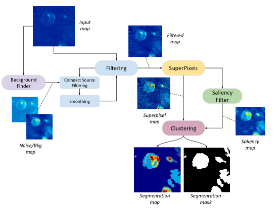
Figure 1: Schematic pipeline of the designed source finder algorithm.

2 The SCORPIO project

The SCORPIO project is a blind deep radio survey of a $2\times 2$ deg² sky patch toward the Galactic plane, using the ATCA array in several configurations. The survey has been conducted at 2.1 GHz between 2011 and 2015 and achieved an average resolution around 10 arcsec. Further observations are already scheduled in 2016. The major scientific goals of the SCORPIO project is to search for different populations of Galactic radio point sources and the study of circumstellar envelopes (related to young or evolved massive stars, planetary nebulae and supernova remnants) which is extremely important for understanding the Galaxy evolution (e.g. ISM chemical enrichment, star formation triggering, etc.). Besides these scientific outputs, SCORPIO will be used as a test-bed for the EMU survey, guiding its design strategy for the Galactic plane sections. In particular, this includes exploring suitable strategies for effectively imaging and extracting sources embedded in the diffuse emission expected at low Galactic latitudes and investigating to what extent they can be employed in the EMU survey.

The SCORPIO observations have produced a radio mosaic map of 133 single pointings with an rms down to 30 $\mu$Jy/beam. A pixel size of 1.5" is chosen for the final map. This sensitivity and a good $uv$-plane coverage have allowed the discovery of about 1000 new faint radio point sources and to satisfactorily map tens of extended sources. Preliminary results on a smaller pilot region of the SCORPIO field have already been published in Paper I, while the complete data reduction and analysis is still in progress.

3 A segmentation method for extended source detection

Detection of extended sources represents a hard task for source finder algorithms. The main difficulties are due to the intrinsic emission pattern, which is usually fainter compared to compact sources (e.g. below the conventional 5$\sigma$ significance level) and spread over disjointed areas (e.g. unlike the adjacency assumption taken in compact source finders). In addition, object borders are usually soft thus the standard edge detector algorithms are not fully sensitive to them. Spatial filters are therefore often employed to enhance the emission at some given scale.

Another issue is related to the estimation of reliable significance levels for detection. In fact, the widely used method for local noise and background estimation is typically biased around extended source regions, namely higher significance levels are artificially imposed for detection with respect to other image regions, free of diffuse emission. Under these conditions the source is likely to be undetected particularly if it has a large extension.

Ideally, the source extraction task should provide a two-level hierarchical information: a segmentation of the input map into background and foreground regions associated with a source object, and, for each of the them, a collection of nested regions representing source features (e.g. clumps, shells, blobs) also at different scales.

To this goal, we designed a multi-stage method based on image superpixel generation and hierarchical clustering. A schematic pipeline of the algorithm stages is shown in Fig. 1 and summarized below:

1. Filtering: To enhance extended structures, bright compact sources need to be filtered out from the map and a residual image generated and used as input for the following stages. Compact source extraction, discussed with more details in Section 3.2, requires the computation of the background and noise maps to threshold the image at a suitable significance level.

   Furthermore, a smoothing stage is introduced on the residual image to suppress texture-like features due to imaging artefacts around the brightest sources and to source residuals left after the previous dilation stage. An edge-preserving guided filter (He et al., 2013) was found to provide optimal performances among the tested filters.

2. Extended source extraction: The smoothed residual image is used as input for the segmentation algorithm described in Section 3.3. It consists of three main stages: firstly, an over-segmentation of the image into a collection of superpixels or regions is generated and a set of appearance parameters (both intensity- and spatial-based) computed for each region; then, a saliency map is computed in the second stage from region dissimilarities and used to drive region merging at the third stage, which is a sequence of clustering steps producing a collection of segmented regions or a binary mask as the final output.

3. Source parametrization: A set of morphological parameters is calculated over the segmented regions and delivered to the user.

Additional details concerning each algorithm step are given in the following sections.

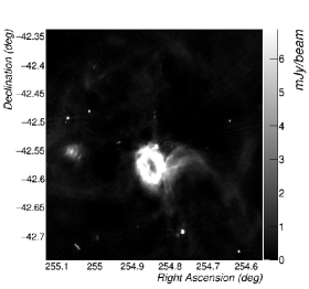
(a) Field A

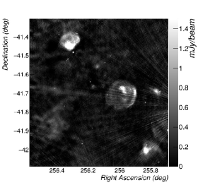
(b) Field B

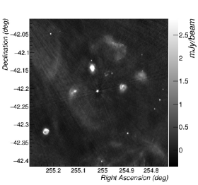
(c) Field C

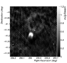
(d) Field D

Figure 2: Sample SCORPIO fields (A-D) selected for algorithm testing. Flux units are reported in the z axis.

3.1 Background and noise estimation

As noted in Paper I, both background and noise levels are subjected to variations throughout the image, due for example to diffuse emission around the Galactic plane or to the accuracy of the image reconstruction. Background and noise information are therefore estimated on a local basis using two alternative methods. The first conventional method assumes a rectangular grid of sample pixels and computes the local background and noise levels over a sampling box, centered around each grid center. Robust background/noise estimators are generally considered to reduce the bias caused by the possible presence of sources falling in the sampling box. For instance Selavy (Whiting, 2009; Whiting & Humphreys, 2012) uses the median and mean absolute deviation from the median (MAD), while the inter-quartile range is adopted in Aegean (Hancock et al., 2012). Other methods use the previous estimators iteratively clipped up to reach a pre-specified tolerance, as in SExtractor (Bertin & Arnouts, 1996) or in Paper I. Several estimators are available in our program: median/MAD, biweight or $\sigma$-clipped estimators. Finally, a bicubic interpolation stage is carried out to derive local estimates on a pixel-by-pixel basis, e.g. the background and noise maps.

The second method exploits the pixel spatial information, neglected by the conventional approach, along with the pixel intensity distribution to produce less biased noise/background estimates. Two different approaches were implemented. In the first, a superpixel partition of the image is generated (see Section 3.3 for more details) with region size assumed comparable to the synthesised beam size. An outlier analysis, based on a robust estimate of the Mahalanobis distance (Rousseeuw & Van Zomeren, 1990) on region median-MAD parameter space, is then performed to detect significative regions (both positive or negative excesses), typically associated with sources or artefacts. Pixels belonging to that regions are marked and excluded from the background evaluation. The background and noise maps are finally computed as above by interpolating a robust estimator computed over background-tagged pixels in sampling boxes sliding through the entire image.

A second approach uses a flood-filling algorithm to detect and iteratively clip blobs at some predefined significance level (e.g. 5$\sigma$) with respect to the first level estimate of the background and noise maps. Background and noise maps are re-computed at each iteration stage as described above. One or two iterations are typically sufficient.

In practice, the first method can be safely used for bright compact source filtering, in which the background estimation is not requested to be highly accurate. The second method should be instead preferred in the search of faint compact sources or when thresholding extended bright sources.

The size of the sampling grid is conventionally chosen to achieve sufficient interpolation accuracy at moderate computational cost. Instead, the choice of the box size is often given in terms of the beam size (e.g. 10 or 20 larger than the synthesised beam) and may have a considerable impact in the source extraction step: estimates computed on a small box could be severely biased by the presence of a source filling the box, while, on the other hand, a too large box could completely smooth out the local background/noise variations. In Huynh et al. (2012) the authors compared maps obtained by popular source finders, such as SFind (Hopkins et al., 2002), SExtractor (Bertin & Arnouts, 1996) and Selavy (Whiting, 2009; Whiting & Humphreys, 2012), and investigated the optimal parameter settings both for real and simulated data sets. However, they note that a completely automated procedure for background estimation, possibly independent on the distribution of sources, is still of crucial importance for future surveys.

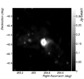
(a)

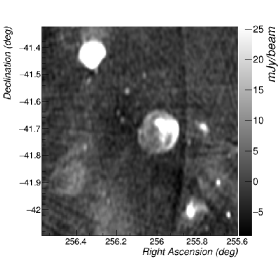
(b)

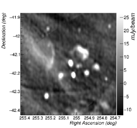
(c)

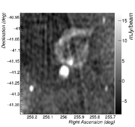
(d)

Figure 3: Sample fields (A-D) selected for algorithm testing as observed in the Molonglo Galactic Plane Survey. Flux units are reported in the z axis.

3.2 Filtering compact sources

The presence of bright sources in the image significantly hardens the extended source detection task. We therefore implemented a filtering stage to remove them, based on the following steps. Blobs of connected pixels are first extracted from the image assuming a flood-filling procedure similar to that carried out in Aegean (Hancock et al., 2012) and Blobcat (Hales et al., 2012) source finders. A high seed threshold above the computed background is assumed, e.g. 10$\sigma$, and pixels are aggregated down to a merge threshold, e.g. 2.6$\sigma$. Each detected blob is subjected to a further search to identify nested blobs. These are extracted by thresholding the image curvature map $\kappa$, obtained by convolving the image with a Logarithm-of-gaussian (LoG) kernel, at some pre-specified threshold level (e.g. $\kappa>$0) or adaptively. A 2-level hierarchy of blobs is finally obtained.

A set of morphological parameters (e.g. contour parameters, moments, shape descriptors, etc), is computed over the detected blobs and selection cuts are applied to identify point-like candidate sources. For example, blobs with a number of pixels that is too large or with an anomalous elongated shape typically fail to pass the point-like cut.

Blobs tagged as "point-like" are removed from the input image using a morphological dilation operator with configurable kernel shape (e.g. elliptic or squared) and size, as suggested in Peracaula et al. (2015), and replaced with a random background realization. A kernel size larger than 5 pixels was assumed to prevent the source halo pixels to further affect the residual image.

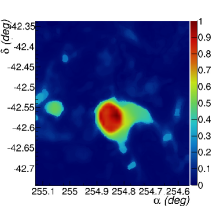
(a) Field A

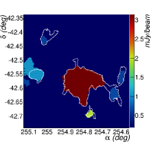
(b) Field A

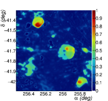
(c) Field B

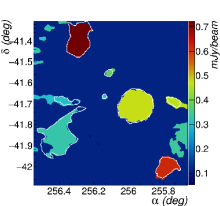
(d) Field B

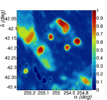
(e) Field C

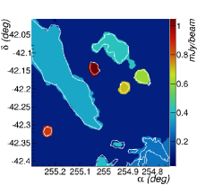
(f) Field C

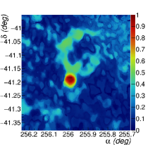
(g) Field D

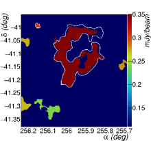
(h) Field D

Figure 4: Segmentation results obtained for the test fields A-D (from top to bottom) assuming $l$=20 and $\beta$=1 (see text). Left: Saliency maps normalized to range [0,1]; Right: Segmentation maps. Each segmented region is colored in the plot according to the mean of its pixel fluxes in mJy/beam units. The white contour lines correspond to a manual segmentation generated by an expert astronomer.

3.3 Segmentation algorithm

We developed a segmentation algorithm for extraction of extended sources, based on a superpixel segmentation algorithm followed by a hierarchical clustering stage to aggregate similar segments into final candidate source regions. The algorithm steps are described below and a summary of the relevant algorithm parameters is reported in Table 1:

1. Initialization: Compute a set of filtered images to be used during the clustering stage, namely the image curvature $\kappa$ and an edge-sensitive map $\psi$. The latter can be alternatively obtained by convoluting the input image with a set of Kirsch filters oriented along different directions or as the result of the Chan-Vese contour finding algorithm (Chan & Vese, 2012).

   

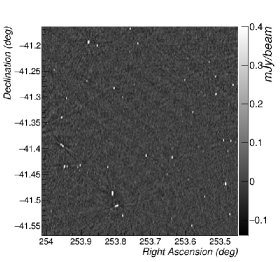
   (a) Field E

   

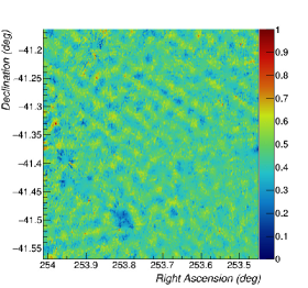
   (b) Field E - Residual

   Figure 5: Left: Sample SCORPIO field E selected for algorithm testing. Flux units are reported in the z axis; Right: Residual map, normalized to range [0,1], obtained after applying point-like source and smoothing filtering stages to the input map.

2. Superpixel segmentation: In this stage the image is over-segmented into $N_{\texttt{R}}$ connected regions or superpixels using flux and spatial information as input observables. To this aim we made use of the Simple linear iterative clustering (SLIC) algorithm developed by Achanta et al. (2012), which uses the k-mean algorithm to cluster pixels according to an intensity and spatial proximity measure. Segmentation is controlled by a set of input parameters, such as the desired superpixel size $l$, typically fixed to the smallest detail to be distinguished (e.g. close to the beam size to detect compact sources or larger to search for extended sources), the minimum number of pixels in a region ($N_{\texttt{min}}$) and a regularization parameter $\beta$ balancing spatial and intensity clustering in the distance measure $D_{ij}$ between a pixel $i$ and a superpixel center $j$:

   $$D_{ij}=\sqrt{D_{ij,c}^{2}+\left(\frac{\beta}{l\times l}\right)^{2}D_{ij,s}^{2}}$$ (1)

   $D_{ij,c}$ and $D_{ij,s}$ being the intensity and spatial Euclidean distances between pixel $i$ and superpixel $j$. Higher $\beta$ enhances the spatial proximity and favors more compact superpixels in the initial partition. In turn, lower $\beta$ favors clustering in intensity and superpixels with less regular shapes but adhering more tightly to the object contours.

   For each region $i$ an appearance parameter vector $\mathbf{x}_{i}=(\mu_{i},\sigma_{i},\mu_{i,\kappa},\sigma_{i,\kappa})$ is computed, with $\mu_{i}$ and $\mu_{i,\kappa}$ denoting respectively the mean of flux and curvature of pixels belonging to region $i$, while $\sigma_{i}$ and $\sigma_{i,\kappa}$ are their standard deviations. With this parameter choice, the computation and update of the region parameters after a merging can be done iteratively in a very fast way, namely without partially sorting the region pixel vector as in the case of median and MAD estimators.

3. Saliency map estimation: A saliency map is estimated in this step to enhance significant objects in the input image with respect to the background. Following Zhang & Ni (2013), a saliency estimator $S_{i}$ is computed for each region as:

   $$S_{i}=1-\exp\left(-\frac{1}{K}\sum_{j=1}^{K}\delta_{ij}\right)\;\;\;\;\;\;\;\;\;\;\;\delta_{ij}=\frac{d_{ij,c}}{1+d_{ij,s}}$$ (2)

   where $d_{ij,c}$ is the Euclidean distance between appearance vectors $\mathbf{x}_{i}$ and $\mathbf{x}_{j}$ of region $i$ and $j$, $d_{ij,s}$ the distance between their centroids. The sum is computed over the $K$ nearest neighbors of region $i$, typically 10% or 20% out of the total number of regions. Salient objects are likely to have similar pixels more confined in space compared to similar pixels belonging to the background which are more spatially spread in the image. To detect salient features at different scales, we combined saliency maps computed at different resolutions, e.g. corresponding to initial partitions with different superpixel sizes. Finally, multi-resolution saliency maps are combined with the computed local noise and background maps, which are found to be also sensitive to the diffuse emission. A saliency map with almost full pixel resolution is finally determined.

4. Superpixel tagging: Each pixel $i$ is tagged as background/object/untagged candidate if its saliency $S_{i}$ is within some adaptive threshold levels:

   $$S_{i}=\left\{\begin{array}[]{ll}\texttt{background}&S_{i}<S_{\texttt{thr}}^{\texttt{bkg}}\vspace{0.2cm}\\ \texttt{object}&S_{i}>S_{\texttt{thr}}^{\texttt{sig}}\vspace{0.2cm}\\ \texttt{untagged}&\text{otherwise}\end{array}\right.$$ (3)

   Different saliency thresholding approaches are possible. One of the most used in saliency studies (Achanta et al., 2009; Perazzi et al., 2012; Kim et al., 2014; Zhang & Ni, 2013) assumes a global adaptive threshold of the kind $S_{\texttt{thr}}^{\texttt{bkg,sig}}=f_{\texttt{thr}}^{\texttt{bkg,sig}}\times\langle S\rangle$, where $\langle S\rangle$ is the average (or median) saliency of the map and $f$ is a numerical factor (e.g. $f$=1 for the background and $f$=2 for the signal; Achanta et al. (2009); Zhang & Ni (2013)). After several tests performed on different maps we obtained optimal results by combining different global threshold measures:

   $$S_{\texttt{thr}}^{\texttt{sig}}=\texttt{max}\{f_{\texttt{thr}}^{\texttt{sig}}\times\langle S\rangle,\texttt{min}\{S_{\texttt{thr}}^{\texttt{Otsu}},S_{\texttt{thr}}^{\texttt{valley}}\}\}$$ (4)

   where $S_{\texttt{thr}}^{\texttt{Otsu}}$ is the threshold level computed through the Otsu method (e.g. see Sezgin & Sankur 2004 for a review of thresholding methods) and $S_{\texttt{thr}}^{\texttt{valley}}$ is the threshold corresponding to the first valley detected in the pixel saliency histogram. The threshold level factor $f_{\texttt{thr}}^{\texttt{sig}}$ is chosen as a trade-off between false detection rate and object detection efficiency. The alternative approach, more computationally expensive, is employing the local adaptive thresholding method used also for compact source extraction with or without outlier rejection.

   Superpixels are finally tagged as background, object or untagged candidates according to the majority of their pixel tags.

5. Superpixel graph: Identify 1st- and 2nd-order neighbors to each region $i$=1,…,$N_{\texttt{R}}$ and build a corresponding link graph as described in Bonev & Yuille (2014). By 1st-order neighbors, we denote the regions surrounding and sharing a border with region $i$. For each region link $i-j$ in the graph, compute an edgeness $E_{ij}$ parameter related to the amount of edge present on the shared border between region $i$ and $j$. For 1st-order neighbors, this is estimated by taking the average of $\psi$ over the pixels located on the shared boundary, while for 2nd-order neighbors, it assumes the largest value present in the $\psi$ map.

   Let us consider an asymmetric dissimilarity measure $\Delta_{ij}$ between neighbor regions $i$ and $j$ given by:

   $$\Delta_{ij}=(1-\lambda)d(\mathbf{x}_{i},\mathbf{x}_{i\cup j})+\lambda E_{ij}$$ (5)

   where $d(\cdot,\cdot)$ is the Euclidean distance between feature vectors, $E_{ij}$ the edgeness parameter and $\lambda$ a regularization parameters balancing distance and edgeness weights in $\Delta_{ij}$.

   The above measure expresses the change of feature vector $\mathbf{x}_{i}$ caused by a potential merging with region $j$, which is favored when the distance between feature vectors is small and penalized when there is a border in between the two regions. Note that $\Delta_{ij}\neq\Delta_{ji}$.

   Compute the adjacency matrix $\mathbf{A}$ of the graph with elements $a_{ij}$:

   $$a_{ij}=\frac{\Delta_{ij}^{-1}}{\sum_{j}\Delta_{ij}^{-1}}$$ (6)

   properly normalized to express a transition probability from node $i$ to $j$.

6. Superpixel merging: Following Ning et al. (2010) and Zhang & Ni (2013), merge superpixels on the basis of a maximum similarity criterion by iterating the following steps until no more merging is possible:

   1. Merge untagged regions to candidate background regions if their similarity is maximal among neighbor similarities.

   2. Adaptively merge untagged regions if their similarity is maximal among neighbors similarities.

   Untagged regions shrink during the previous stage, while background regions grow. Signal-tagged regions are not affected in the previous stages. Superpixel parameter vector and graph (neighbor links, dissimilarity/adjacency matrix) are updated after each iterated merging stage. When no more merging is favored, all the remaining untagged regions are labeled as signal candidates. This stage always converges to assign all regions to either background or signal.

   A suitable superpixel merging order for each of the steps described above is determined as in Bonev & Yuille (2014) using the Google PageRank algorithm (Brin & Page, 1998) on the transition matrix $A$, that is solving the following equation:

   $$\mathbf{p}=(1-d)\mathbf{e}+d\mathbf{A}^{T}\mathbf{p}$$ (7)

   in which $\mathbf{p}=(p_{1},p_{2},\dots,p_{N_{\texttt{R}}})$ is the desired vector with rank values (the principal eigenvector of $\mathbf{A}$), $d$ is the damping factor which can be set to a value between 0 and 1 (e.g. $d$=0.85 as in Brin & Page (1998); Page et al. (1999)) and $\mathbf{e}$ is a column vector of all 1’s. The equation is solved by using the power iteration method (Golub & Van Loan, 1983). $\mathbf{p}$ is sorted and allows to select nodes with higher ranks for merging.

7. Source selection: In this step sources are identified from the collection of signal candidate regions selected in the previous stage. Following Bonev & Yuille (2014) the most similar signal regions are hierarchically clustered if their mutual dissimilarities ($\Delta_{ij}$, $\Delta_{ji}$) are within a pre-specified tolerance. Only a percentage (e.g. 30%) of top ranked merging are allowed at each clustering iteration.

   A practical criterion for the merging is allowing first neighbors to always merge (e.g. a sort of flood-fill approach over superpixels) and assuming a tolerance for 2nd-order neighbors. Region parameter vectors and the dissimilarity/adjacency matrix are updated at each iteration stage and stop conditions are checked. If no regions are merged at the current hierarchy level or the remaining number of regions is below a specified threshold the algorithm stops and the final segmentation is returned to the user, otherwise a new iteration is started.

8. Post-processing: Some post-processing stages can be performed on the detected sources. A first step uses the hierarchical clustering approach described above to identify similar regions within each source and generate a list of nested sources one level down in the source hierarchy. Further, following Yang et al. (2008), a number of statistical and morphology-descriptor parameters are computed over the source contour and/or its pixel distribution to be eventually employed in a source classification stage. Standard parameters include bounding box/ellipse, image/contour moments and roundness/rectangularity estimators. More complex parameters, such as Fourier Descriptors (FDs) (Zhang & Lu, 2003), Hu (Hu, 1962) and Zernike moments (Singh & Walia, 2011), can be computed and supplied to the user.

Table 1: Main parameters used in the source finder algorithm.

Stage	Parameter	Description
Background	bkgModel	Model to be used for computing the background and noise maps (1=global, 2=local, 3=local robust).
	boxSize	Size of the box used to compute local background/noise estimators.
	gridSize	Size of the grid used when interpolating the local background/noise estimators.
Filtering	$\sigma_{\texttt{seed}}$ $\sigma_{\texttt{merge}}$	Seed and merge threshold used to detect compact bright blobs in the image, e.g. $\sigma_{\texttt{seed}}$=10, $\sigma_{\texttt{merge}}$=2.5.
	$K_{\texttt{dilate}}$	Kernel size to be used when dilating bright sources.
	$\sigma_{\texttt{smooth}}$ $K_{\texttt{smooth}}$	Kernel and radius parameter to be used in image residual smoothing.
Superpixel Generation	$l$	Superpixel size used to generate the initial superpixel partition.
	$\beta$	Regularization parameter controlling starting superpixel segmentation and balancing clustering spatial and color distance. Low $\beta$ values favors spatial clustering, high $\beta$ favors color clustering
Saliency Filter	$l_{\texttt{min/max/step}}$	Superpixel sizes to be used in multi-resolution saliency computation, e.g. $l$=20-60, step 10.
	knn	Fraction of nearest neighbors superpixel used in saliency estimation, e.g. knn=10%/20%
	$f_{\texttt{sal}}^{\texttt{scales}}$	Fraction of salient scales required to contribute to final saliency estimation, e.g. knn=70%
	useCurvMap	Flag to include (multi-scale) curvature maps in saliency estimation
	useBkgMap	Flag to include (multi-scale) background map in saliency estimation
	useNoiseMap	Flag to include (multi-scale) noise map in saliency estimation
	salThrModel	Method to be used for thresholding final saliency map (1=global, 2=local, 3=local robust)
	$f_{\texttt{thr}}^{\texttt{bkg}}$	Global threshold parameter to tag background pixel candidates in saliency map, e.g. $f_{\texttt{thr}}^{\texttt{bkg}}$=1.
	$f_{\texttt{thr}}^{\texttt{sig}}$	Global threshold parameter to tag signal pixel candidates in saliency map, e.g. $f_{\texttt{thr}}^{\texttt{bkg}}$=2.
Superpixel Merging	$\lambda$	Regularization parameter used in superpixel merging stage balancing appearance and edge terms when computing superpixel dissimilarities. Low $\lambda$ values (close to zero) favors intensity similarity, high $\lambda$ values (close to 1) favors edge penalization.
	Edge Model	Model to be used to compute superpixel edgeness (1=Kirsch, 2=Chan-Vese).
	$f_{\texttt{merge}}$	Fraction of top ranked superpixels selected for merging at each hierarchy level, e.g. $f_{\texttt{merge}}$=30%.
	$\varepsilon_{\texttt{merge}}^{\texttt{1st,2nd}}$	Maximum mutual dissimilarity tolerance used for accept a selected superpixel merging for 1st or 2nd neighbor superpixels, e.g. 5-15%.
	$\Delta_{\texttt{thr}}$	Absolute dissimilarity threshold, when applied, to select/reject selected superpixel merging ($\Delta_{ij}\leq\Delta_{thr}$). Low $\Delta_{thr}$ values (close to zero) imply strict superpixel similarity for merging. High $\Delta_{thr}$ values relax the merging.

3.4 Algorithm implementation

The described algorithms have been implemented in a C++ software library, dubbed CAESAR (Compact And Extended Source Automated Recognition), allowing image filtering, background estimation, source finding, image segmentation starting from images in FITS or ROOT format. The library is mainly based on the ROOT (Brun & Rademakers, 1997) and R (R Core Team, 2014) frameworks for statistical objects and methods and on the OpenCV library (Bradski, 2000) for some of the image filtering algorithms. The source finding and segmentation algorithms have been developed from scratch along with some of the employed filtering stages. Future developments include the algorithm fine-tuning and optimization and further design activities for ease of deployment in a distributed computing infrastructure and integration within the pipeline frameworks of next-generation telescopes. Public distribution is planned once optimization steps are carried out.

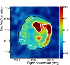
(a) Field B

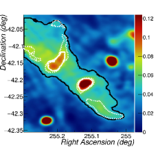
(b) Field C

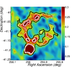
(c) Field D

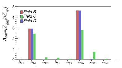
(d)

Figure 6: Top panels: Sample segmented source images, normalized to range [0,1], in field B, C and D (solid black contours). White contours represent nested regions selected with a multi-resolution saliency-based method (solid lines) and with a multi-scale blob detector (dashed lines); Bottom panels: Zernike moments up to order $n$=4 computed over the segmented sources shown in the upper panels (black contoured area).

4 Application to SCORPIO project data

4.1 Sample fields

To test the designed algorithm we considered four selected fields from the SCORPIO map in which several extended structures are present along with compact sources. The map is built as described in Paper I using data observed with the ATCA 0.75A array configuration in combination with data observed with the ATCA EW367 configuration, in which shorter baselines are present. The effective frequency range of the radio data used is 1.4-3.1 GHz. The sample fields, hereafter denoted as field A-D are shown in Fig. 2, and some details are reported below:

• Field A (Fig. 2a): Field A (1000$\times$1000 pixels) is centered on the [DBS2003] 176 galactic stellar cluster (l=343.4830^∘, b=-00.0380^∘, angular size=1.45 arcmin). Two bubble objects, S16 and S17 (Churchwell et al., 2006), are associated with the cluster but only S17 is observed in the radio domain. Two bright point-like radio sources (SCORPIO1_320 and SCORPIO1_300), already known objects in radio, were identified in Paper I. SCORPIO1_300 is located within the S17 bubble and has peak flux around 0.04 Jy/beam. The brighter SCORPIO1_320 (peak flux$\sim$0.14 Jy/beam) has been tentatively classified as a Massive Young Stellar Object (MYSO) candidate (Urquhart et al., 2007).

• Field B (Fig. 2b): Field B (1600$\times$1850 pixels) is centered on the Supernova Remnant (SNR) G344.7-0.1, located in the adjacency of the high energy $\gamma$-ray source HESSJ1702-420 (see Giacani et al. 2011). Close to the SNR, in the north-east region of the image, another extended emission is present and most probably associated with the MSC 345.1-0.2 supernova remnant candidate ($l$=345.062, $b$=-0.218 according to the MOST MSC survey at 843 MHz (Whiteoak & Green, 1996)).

• Field C (Fig. 2c): Field C (1000$\times$1000 pixels) was analyzed in detail in Paper I. Some of the extended regions of emission present were associated with the following IRAS sources: IRAS 16566-4204, IRAS 16573-4214, IRAS 16561-4207. The first is recognized as a massive star formation region, while classification is uncertain for the others.

• Field D (Fig. 2d): Field D (1000$\times$1000 pixels) is centered on the faint SNR Candidate MSC G345.1+0.2. Below this a more intense emission is present, associated with the G345.097+00.136 HII region.

An additional control field, free of extended sources and denoted as field E, is considered to study the algorithm response in the absence of any expected signal and tune the detection thresholds. Field E is reported in Fig. 5 (left panel). This map is built using data observed with the ATCA 0.75A array configuration alone. Due to the larger minimum baseline available extended and diffuse sources are strongly filtered out.

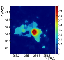
(a) Field A

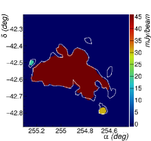
(b) Field A

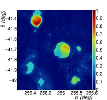
(c) Field B

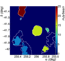
(d) Field B

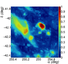
(e) Field C

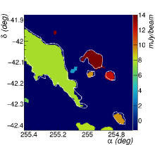
(f) Field C

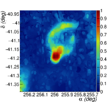
(g) Field D

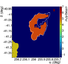
(h) Field D

Figure 7: Segmentation results obtained for the Molonglo sample fields A-D (from top to bottom) assuming $l$=5 and $\beta$=1. Left: Saliency maps normalized to range [0,1]; Right: Segmentation maps. Each segmented region is colored in the plot according to the mean of its pixel fluxes in mJy/beam units. The contours shown with solid white lines correspond to a manual segmentation generated by an expert astronomer.

As discussed in Paper I the regions of extended emission present in the test fields A-D are in a few cases firmly associated with real source objects or candidates. In most cases, however, no association with known sources has been established and an artefact nature cannot be excluded a priori without a further insight and comparison to other surveys carried out with different telescopes or wavelength domains. As a result, no ground truth information at pixel level is available to quantify the algorithm performances in terms of widely used measures, such as the identification efficiency and false detection rate. The quality of the reconstruction will be therefore compared to a human-driven segmentation generated for each sample image by an expert astronomer. To enhance the source/artefact discrimination capabilities, we considered the same sample scenarios as observed in the Molonglo Galactic Plane Survey (MGPS) at 843 MHz, reported in Fig. 3. The rms sensitivity over the survey is around 1-2 mJy/beam and the positional accuracy is 1-2". The lower resolution appears evident, particularly in Field B and C in which some of the extended regions present in SCORPIO are not fully resolved and are detected as compact sources in the source finding stage. On the other hand, due to the lower observing frequency, regions of extended emission are brighter and can be detected at higher significance levels. Furthermore, it is unlikely that the same imaging artefacts appear in both surveys which are conducted with different telescopes. Thus, common emission features can be therefore considered as real with a high degree of confidence.

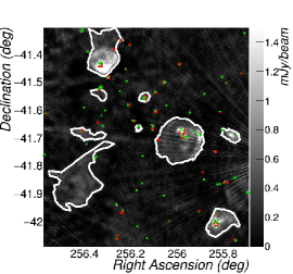
(a) Field B - Aegean, Blobcat

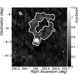
(b) Field D - Aegean, Blobcat

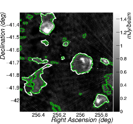
(c) Field B - Chan-Vese

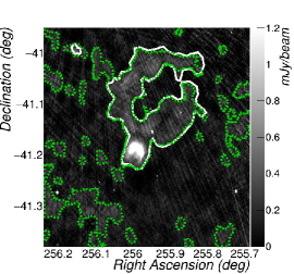
(d) Field D - Chan-Vese

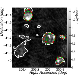
(e) Field B - SWT

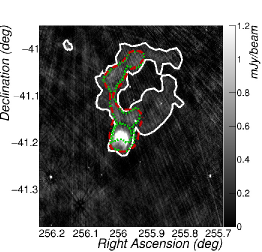
(f) Field D - SWT

Figure 8: Source finding results obtained with three different algorithms over field B (left panels) and field D (right panels) compared to the human segmentation (solid white contours); Top: Results obtained with the Aegean (dotted green contours) and Blobcat source finders (dashed red contours); Center: Results obtained with the Chan-Vese algorithm (dotted green contours); Right: Results obtained with the Stationary Wavelet Transform (SWT) method at scale $J$=5 (dotted green contours) and $J$=6 (dashed red contours).

4.2 Results

We applied the designed segmentation algorithm to the selected test fields described in Section 4.1. Multiple runs were performed under different choices of the algorithm parameters. The quality of the segmentation was visually inspected against the human segmentation and a suitable choice of the algorithm parameters selected on the basis of the maximum number of expected objects detected in all test fields at the corresponding minimum false detection rate.

A minimum region size $l$ for the initial segmentation equal to $l\sim 4\times$beam (equivalent to $l$=20 pixels) was considered. Smaller values (e.g. $l$=10 pixels), comparable to the beam size, were found to be too sensitive to small-scale structures (residual compact emission, artefacts) in the image and thus provide noisy segmentation results. Larger values, e.g. $l$=30-60 pixels, were investigated as well. As $l$ increases, small-scale details of the extended sources may be smoothed out. This does not represent an issue for field A and B in which the extended emission scale is larger by a factor of 4-5 compared to the minimum region size. Furthermore a larger value of $l$ favors the merging of artefacts in the background region, e.g. in Field B.

The regularization parameter $\beta$, controlling initial over-segmentation, was studied. Different values were considered ($\beta$=0.01, 1, 10, 100) in correspondence to all other scanned parameters. Results were found comparable for $\beta$=0.01-1 while for values above $\beta$=10 the superpixels start to assume very compact shapes and does not fit well to object boundaries.

The saliency maps computed for the SCORPIO sample fields using a multi-resolution range of $l$=20-60 pixels (step 10 pixels), in combination with background and noise maps, are shown in the left panels of Fig. 4. It can be noted how the faint diffuse emission, previously hardly detectable without manually adjusting the map contrast, is significantly enhanced over the background after the saliency filter. The filter mostly preserves the expected object contours and slightly smooth out small scale details. A thresholding procedure on these saliency maps provides the initial signal and background markers for the following algorithm stages. Suitable values of the global signal threshold factor $f_{\texttt{thr}}^{\texttt{sig}}$ were searched over all test samples. The choice of the threshold level was mainly driven by Field D and control Field E and optimal values were found in the range 2.5-2.8. Higher values (up to 3.0) can be given to other fields at the cost of missing parts of the faint SNR source in Field D and of the large diffuse emission in Field C. Overall, we have found that the thresholded saliency map alone already provides a reasonable source detection. It is also worth to observe that saliency maps may constitute a valid input for different algorithms.

Different choices of the similarity regularization parameter $\lambda$ were investigated: $\lambda$= 0, 0.1, 0.5. Results obtained with $\lambda$=0.1, 0.5 are overall comparable, with slightly better results obtained with $\lambda$=0.5, while worse results are obtained with $\lambda$=0. This analysis demonstrates that incorporating an edge information in the algorithm improves the segmentation quality, even though edges of radio objects are considerably softer than in natural images.

The results of the segmentation stage are reported in the right panels of Fig. 4 for the four tested fields assuming $l$=20 pixels, $\beta$=1 and $\lambda$=0.5. Each segmented region is colored according to the mean of its pixel fluxes. The human segmentation is superimposed and shown with solid white contours. As it can be seen known objects and regions of diffuse emission are all identified and kept for later post-processing. The algorithm, at least with this choice of parameters, is also sensitive to other faint diffuse emission which were not identified in the human segmentation. After a deeper inspection, some of these were clearly attributed to imaging artefacts present in the input map, particularly in the field B in which a poorly cleaned bright object outside the studied field pollutes the entire map. For the remaining objects the nature remains unclear even after a visual inspection. This kind of artefacts represents a limitation in current SCORPIO map release. They can be removed in our analysis by increasing the threshold levels in the saliency map, at the cost of affecting source detection especially in fields C and D.

In Fig. 5 (right panel) we report the results obtained over test field E using the same algorithm parameters selected for fields A-D. The left panel shows the input map while the right panel the map given to the segmentation algorithm after the compact source filtering and smoothing stage. As desired, no signal markers are found in the saliency map and thus no extended source detection is reported.

An example of post-processing analysis, carried out for some relevant sources present in the test fields, is reported in Fig. 6. Top panels shows the identified sources (solid black line contours) with nested components detected using two different methods. Solid white line contours are obtained by thresholding a multi-resolution saliency map computed over source pixels. Dashed white line contours are produced by a multi-scale blob detector approach, combining Laplacian of Gaussian (LoG) image filters at different scales. Other analysis are possible with the designed algorithm, e.g. running the hierarchical clustering over the source region to identify the most similar areas, thus not shown here.

As discussed in Section 3.3 a set of parameters can be computed for each detected source, even the nested ones. As an example we report in the bottom panel of Fig. 6 the set of Zernike moments computed for the three sources up to the 4-th order. Note how the moments are sensitive to the source morphology and can be in principle considered for classification studies in combination with the other computed parameters (not in this paper purposes). A study of the suitable set of parameters and their robustness to noise is planned to be performed using simulated data.

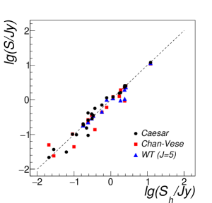
Figure 9: Integrated fluxes $S$ of extended sources in the test fields A-D, reconstructed with three different algorithms (black dots: CAESAR, red squares: Chan-Vese, blue triangles: Wavelet Transform J=5), as a function of the human-driven segmentation flux $S_{h}$.

4.3 Application to data at different wavelengths

To evaluate the results obtained on radio data collected at different wavelengths and detector resolutions/sensitivities we considered the same test scenarios as observed in the Molonglo Galactic Plane Survey (MGPS) at 843 MHz, shown in Fig. 3. We applied our method to the sample Molonglo fields using the same parameters considered in the analysis of the SCORPIO fields, with the following exceptions related to the lower resolution and size of the Molonglo maps. Smaller values of the superpixel sizes ($l$=5-10 pixels) can be assumed with respect to the SCORPIO maps, in which we have considered a minimum value of $l$=20 pixels. Saliency maps have been therefore computed starting from the chosen minimum superpixel size up to a smaller maximum scale value compared to that assumed in SCORPIO maps. A less aggressive initial smoothing filter is also assumed in this case. All the other algorithm parameters are left unchanged. The results are reported in Fig. 7. Some of the extended sources present in the field are not resolved and are detected as compact sources in the pre-filtering stage. The white contours shown in the plots are therefore relative to the detectable extended sources. As it can be seen, all the known sources are detected with high fidelity when comparing to the superimposed human segmentation. Additional regions of diffuse emission are detected as well. It is unclear at the present status whether they are real or most probably reconstruction artefacts. Overall, the results demonstrate that the method is flexible to be used also with different data under a minor tuning of parameters driven by the data itself, mainly sensitivity and resolution.

4.4 Results with different algorithms

It is valuable to consider what can be achieved on SCORPIO observed fields with other existing algorithms. Such a test is indeed useful to be carried out as many of the available algorithms were tested with less-sensitive radio data or benchmarked against simulated data neglecting the real background behavior and the Galactic Plane diffuse emission.

Four different methods were considered and tested. The first two, Aegean (Hancock et al., 2012) and Blobcat (Hales et al., 2012) use a flood-fill algorithm to detect blobs in the image, starting from pixels above a seed threshold $\sigma_{\texttt{seed}}$ ($\sigma_{\texttt{seed}}$=5) with respect to the background and aggregating adjacent pixels above a second lower threshold $\sigma_{\texttt{merge}}$ ($\sigma_{\texttt{merge}}$=2.6). Blobs are finally deblended using curvature information. Background and noise maps were computed using the BANE tool distributed within the Aegean source finder. A third method, adopted by Peracaula et al. (2011), searches for blobs on the Stationary Wavelet Transform (SWT) of a residual image, obtained from the input map by replacing bright compact sources with a random background estimate. We implemented this method from scratch. Finally an implementation of the Chan-Vese active contour algorithm (Chan & Vese, 2012) was considered and tested over the sample data. The method iteratively evolves an initial contour till convergence on the boundaries of the foreground region. Contour evolution is done by seeking a level set function that minimizes a fitting energy functional depending on a set of input parameters.

In Fig. 8 we report the sources detected by the four methods (from top to bottom) in fields B (left panels) and D (right panels) in comparison with the human segmentation shown with solid white contours. Aegean and Blobcat results are comparable. As expected, both algorithms were found to perform very well to detect bright and faint compact sources, including blended sources, but they are biased, by design, against extended sources. A 5$\sigma$ threshold was considered for source detection with the Wavelet method on two different scales $J$=5, 6. In these conditions, most of the extended bright sources present in the fields can be detected. Fainter features, such as parts of the supernova remnants or diffuse regions cannot be well detected, at least at the specified significance level.

The Chan-Vese algorithm was tested over the residual image under different choices of parameters and using a simple circular level-set as initial contour. A pre-smoothing stage is applied to the input residual image. Contours surrounding areas of negative excesses with respect to the background level were removed from the set of final detected contours. As it can be seen, the extended source features missed by the other algorithms can be extracted with high accuracy compared to the human segmentation. Some imaging artefacts are also detected along with real sources even with the optimal choice of the Chan-Vese parameters. Overall, the Chan-Vese method was found to outperforms the other three tested algorithms in fully detecting extended objects.

In Fig. 9 we compare the integrated flux of the extended sources present in the four fields A-D estimated with three different methods (CAESAR: black dots, Chan-Vese: red squares, Wavelet method at scale $J$=5: blue triangles) as a function of the flux estimated using the human-driven segmentation. A total of 30 source candidates were identified, hereafter denoted as the "reference set". Data are reported in the plot for each algorithm in case of source identification and cross-match found with the reference set. As it can be seen, the estimated fluxes closely follow the reference, the observed spread in flux being regarded as a measure of the source reconstruction accuracy contribution to the total flux uncertainty. Overall, better results are obtained with the CAESAR and Chan-Vese algorithm, which are able to detect fainter sources with respect to the Wavelet method and achieve a better accuracy in flux estimation.

We are aware that we have not exhausted the list of all possible algorithms for extended source extraction and that a deeper tuning is needed for the three tested algorithms before drawing firm conclusions on their suitability for our goals. For instance, a more refined initialization strategy is desired in the Chan-Vese method together with a finer exploration of the parameter space. Moreover, it is known that the two-level assumption (foreground/background) at the basis of the standard Chan-Vese algorithm may not be accurate to scenarios in which a large variation of intensity levels is present. New active contours algorithms (Vese & Chan, 2002; Yang et al., 2013), overcoming some of the standard Chan-Vese limitations, appeared recently in the literature and could be worthy of consideration. However, we expect that none of the methods will perform accurately over all the presented images and that a combination of different techniques is probably required at the very end. That motivated the development of a completely different approach reported in this paper.

5 Summary

We described in this paper a new algorithm for the detection of extended sources in radio maps, designed for the SCORPIO project and for next-generation radio surveys. The algorithm was tested with real radio data observed in the SCORPIO and Molonglo surveys and compared with existing algorithms. The achieved performances are found comparable or even superior to other approaches followed in the literature. The novel points introduced are:

• a new procedure for computing the background in presence of extended emission;

• an efficient filter to enhance diffuse emission, based on compact bright source removal, smoothing and saliency estimation;

• a flexible framework providing rich information for post-processing analysis and relaxing some of the limiting requirements used for compact source detection (e.g. pixel adjacency)

The results obtained with real data are promising and motivate further work both on the data side and on the algorithm side.

For this purpose, a new release of the SCORPIO map, with improved cleaning procedure and data flagging applied, is in progress. Preliminary results on the studied fields show that many of the artefacts present in the first data release are now properly removed. Further, a campaign of single-dish measurement in the SCORPIO field is already scheduled to improve the map response to extended objects beyond the limits of the ATCA telescope. Source finding will therefore largely benefit from these improved maps.

At the same time, simulation activities were started with the aim of generating extended source mock scenarios with ground truth available at pixel level to study the achieved source detection efficiency and contamination rate with realistic noise conditions.

We are currently working on possible significant improvements also on the algorithm side, both at code and method level. Among these, improving saliency estimation and resolution has become an active field of development in recent works, see Perazzi et al. (2012); Cheng et al. (2014); Borji et al. (2014); Shi et al. (2015). A proper combination of different algorithms could be a viable solution to decrease the spurious detection rate. Suitable criteria for combining nearby candidate sources is another aspect to be investigated in detail.

The current algorithm implementation is not optimized for large maps, e.g. the full SCORPIO or expected ASKAP fields, as it still requires large computation time, e.g. from few to $\sim$15-20 minutes depending on image size, and memory requirements even on a single field, mainly related to the superpixel similarity matrixes. A new optimized version, also designed for parallel and/or distributed processing is therefore planned to be realized, possibly compliant with ASKAP EMU software pipeline requirements in terms of input/output products to be supported, employed technologies and processing strategies (Cornwell et al., 2011; Chapman et al., 2014).

References

- Achanta et al. (2009) Achanta R. et al., 2009, Proc. of the IEEE Conference on Computer Vision and Pattern Recognition (CVPR), Miami, FL, p. 1597
- Achanta et al. (2012) Achanta R. et al., 2012, IEEE Trans. Pattern Anal. Mach. Intell., 34, 2274
- Alexander et al. (2009) Alexander P. et al., 2009, in Torchinsky S.A., van Ardenne A., van den Brink-Havinga T., van Es A.J.J., Faulkner A.J., eds, Proc. of the Wide Field Science and Technology for the SKA Conference, Chateau de Limelette, Belgium, p. 119
- Bertin & Arnouts (1996) Bertin E., Arnouts S., 1996, A&AS, 117, 393
- Bonev & Yuille (2014) Bonev B., Yuille A. L., 2014, in Lecture Notes in Computer Science Ser. Vol. 8691, Proc. of the European Conference on Computer Vision (ECCV), Zürich, Switzerland, p. 535
- Borji et al. (2014) Borji A. et al., 2014, preprint (arXiv:1411.5878)
- Bradski (2000) Bradski G., 2000, Dr. Dobb’s Journal of Software Tools, record: citeulike:2236121. See also http://opencv.org/
- Brin & Page (1998) Brin S., Page L., 1998, Computer Networks, 30, 107
- Brun & Rademakers (1997) Brun R., Rademakers F., 1997, in Nucl. Inst. and Meth. in Phys. Res. A 389, Proc. of the AIHENP’96 Workshop, Lausanne, Switzerland, p. 81. See also http://root.cern.ch/
- Chan & Vese (2012) Chan T. F., Vese L., 2001, IEEE Trans. Image Process. 10, 266-277
- Chapman et al. (2014) Chapman J. at al., 2014, CSIRO ASKAP Science Data Archive: Overview, Requirements and Use Cases, ASKAP-SW-0017
- Cheng et al. (2014) Cheng M. M. et al., 2014, IEEE Trans. Pattern Anal. Mach. Intell., 37, 3
- Churchwell et al. (2006) Churchwell E. et al., 2006, ApJ, 649, 759
- Cornwell et al. (2011) Cornwell T. et al., 2011, ASKAP Science Processing, ASKAP-SW-0020
- Dabbech et al. (2015) Dabbech A. et al., 2015, A&A, 576, A7
- Giacani et al. (2011) Giacani E. et al., 2011, A&A, 531, A138
- Golub & Van Loan (1983) Golub G. H., Van Loan C. F., 1983, Matrix Computations, The Johns Hopkins University Press, Baltimore, MD
- Hales et al. (2012) Hales C. A. et al., 2012, MNRAS, 425, 979
- Hancock et al. (2012) Hancock P. J. et al., 2012, MNRAS, 422, 1812
- He et al. (2013) He K. et al., 2013, IEEE Trans. Pattern Anal. Mach. Intell., 35, 6
- Hollitt & Johnston-Hollitt (2012) Hollitt C., Johnston-Hollitt M., 2012, Publ. Astron. Soc. Australia, 29, 309
- Hopkins et al. (2002) Hopkins A. M. et al., 2002, AJ, 123, 1086
- Hopkins et al. (2015) Hopkins A. M., Whiting M. T., Seymour N. et al., 2015, Publ. Astron. Soc. Australia, 32, e037
- Hu (1962) Hu M., 1962, IRE Trans. Inf. Theory 8, 179
- Huynh et al. (2012) Huynh M. T. et al., 2012, Publ. Astron. Soc. Australia, 29, 229
- Kim et al. (2014) Kim J. et al., 2014, Proc. of the IEEE Conference on Computer Vision and Pattern Recognition (CVPR), Columbus, OH, p. 883
- Kitaeff et al. (2014) Kitaeff V. V. et al., 2014, A&C, 6, 41
- Kitaeff et al. (2015) Kitaeff V. V. et al., 2015, A&C, 12, 229
- Ning et al. (2010) Ning J. et al., 2010, Pattern Recognition, 43, 445
- Norris et al. (2011) Norris R. et al., 2011, Publ. Astron. Soc. Australia, 28, 215
- Norris et al. (2013) Norris R. et al, 2013, Publ. Astron. Soc. Australia, 30, 20
- Page et al. (1999) Page L. et al., 1999, Technical Report 1999-0120, Computer Science Department, Stanford University
- Peracaula et al. (2011) Peracaula M. et al., 2011, Proc. of the 18th IEEE International Conference on Image Processing (ICIP), Brussels, Belgium, p. 2805
- Peracaula et al. (2015) Peracaula M. et al., 2015, New Astronomy, 36, 86
- Perazzi et al. (2012) Perazzi F. et al., 2012, Proc. of the IEEE Conference on Computer Vision and Pattern Recognition (CVPR), Providence, RI, p. 733
- R Core Team (2014) R Core Team, 2015, R: A language and environment for statistical computing. R Foundation for Statistical Computing, Vienna, Austria. See also http://www.R-project.org/
- Röttgering et al. (2010) Röttgering H. et al., 2010, http://www.astron.nl/radio-observatory/apertif-eoi-abstracts-and-contact-information
- Rousseeuw & Van Zomeren (1990) Rousseeuw P. J., Van Zomeren B. C., 1990, Journal of the American Statistical Association, 85, 633
- Sezgin & Sankur (2004) Sezgin M., Sankur B., 2004, Journal of Electronic Imaging, 13, 146
- Shi et al. (2015) Shi J. et al., 2015, preprint (arXiv:1408.5418)
- Singh & Walia (2011) Singh C., Walia E., 2011, Image and Vision Computing, 29, 251
- Umana et al. (2015) Umana G. et al., 2015, MNRAS, 454, 902
- Urquhart et al. (2007) Urquhart J. S. et al., 2007, A&A, 461, 11
- Van der Heyden & Jarvis (2010) Van der Heyden K., Jarvis M. J., 2010, MIGHTEE proposal to Meerkat
- Vese & Chan (2002) Vese L., Chan T. F., 2002, International Journal of Computer Vision, 50, 271
- Whiteoak & Green (1996) Whiteoak J. B. Z., Green A. J., 1996, A&AS, 118, 329
- Whiting (2009) Whiting M. T., 2009, MNRAS, 421, 3242
- Whiting & Humphreys (2012) Whiting M. T., Humphreys B., 2012, Publ. Astron. Soc. Australia, 29, 371
- Yang et al. (2008) Yang M. et al., 2008, Pattern Recognition, IN-TECH, 43
- Yang et al. (2013) Yang Y. et al., 2013, Proc. of the 7th International Conference on Image and Graphics (ICIG), Qingdao, China, p. 201
- Zhang & Lu (2003) Zhang D., Lu G., 2003, J. Vis. Commun. Image R., 14, 41
- Zhang & Ni (2013) Zhang Y., Ni S., 2013, Journal of Computational Information Systems, 9, 3603