Asymmetric Rényi Problem and PATRICIA Tries

Abstract

Abstract:

In 1960 Rényi asked for the number of random queries necessary to recover a hidden bijective labeling of $n$ distinct objects. In each query one selects a random subset of labels and asks, what is the set of objects that have these labels? We consider here an asymmetric version of the problem in which in every query an object is chosen with probability $p>1/2$ and we ignore “inconclusive” queries. We study the number of queries needed to recover the labeling in its entirety (the height), to recover at least one single element (the fillup level), and to recover a randomly chosen element (the typical depth). This problem exhibits several remarkable behaviors: the depth $D_{n}$ converges in probability but not almost surely and while it satisfies the central limit theorem its local limit theorem doesn’t hold; the height $H_{n}$ and the fillup level $F_{n}$ exhibit phase transitions with respect to $p$ in the second term. To obtain these results, we take a unified approach via the analysis of the external profile defined at level $k$ as the number of elements recovered by the $k$th query. We first establish new precise asymptotic results for the average and variance, and a central limit law, for the external profile in the regime where it grows polynomially with $n$. We then extend the external profile results to the boundaries of the central region, leading to the solution of our problem for the height and fillup level. As a bonus, our analysis implies novel results for random PATRICIA tries, as it turns out that the problem is probabilistically equivalent to the analysis of the height, fillup level, typical depth, and external profile of a PATRICIA trie built from $n$ independent binary sequences generated by a biased($p$) memoryless source.

1 Introduction

In his lectures in the summer of 1960 at Michigan State University, Alfred Rényi discussed several problems related to random sets [21]. Among them there was a problem regarding recovering a labeling of a set $X$ of $n$ distinct objects by asking random subset questions of the form “which objects correspond to the labels in the (random) set $B$?” For a given method of randomly selecting queries, Rényi’s original problem asks for the typical behavior of the number of queries necessary to recover the hidden labeling.

Formally, the unknown labeling of the set $X$ is a bijection $\phi$ from $X$ to a set $A$ of labels (necessarily with equal cardinality $n$), and a query takes the form of a subset $B\subseteq A$. The response to a query $B$ is $\phi^{-1}(B)\subseteq X$.

Our contribution in this paper is a precise analysis of several parameters of Rényi’s problem for a particular natural probabilistic model on the query sequence. In order to formulate this model precisely, it is convenient to first state a view of the process that elucidates its tree-like structure. In particular, a sequence of queries corresponds to a refinement of partitions of the set of objects, where two objects are in different partition elements if they have been distinguished by some sequence of queries. More precisely, the refinement works as follows: before any questions are asked, we have a trivial partition ${\mathfrak{P}}_{0}=X$ consisting of a single class (all objects). Inductively, if ${\mathfrak{P}}_{j-1}$ corresponds to the partition induced by the first $j-1$ queries, then ${\mathfrak{P}}_{j}$ is constructed from ${\mathfrak{P}}_{j-1}$ by splitting each element of ${\mathfrak{P}}_{j-1}$ into at most two disjoint subsets: those objects that are contained in the preimage of the $j$th query set $B_{j}$ and those that are not. The hidden labeling is recovered precisely when the partition of $X$ consists only of singleton elements. An instance of this process may be viewed as a rooted binary tree (which we call the partition refinement tree) in which the $j$th level, for $j\geq 0$, corresponds to the partition resulting from $j$ queries; a node in a level corresponds to an element of that partition. A right child corresponds to a subset of a parent partition element that is included in the subsequent query, and a left child corresponds to a subset that is not included. See Example 1 for an illustration.

Example 1 (Demonstration of partition refinement).

Consider an instance of the problem where $X=[5]=\{1,...,5\}$, with labels $(d,e,a,c,b)$ respectively (so $A=\{a,b,c,d,e\}$). Consider the following sequence of queries:

1. $B_{1}=\{b,d\}\mapsto\{1,5\}$

2. $B_{2}=\{a,b,d\}\mapsto\{1,3,5\}$,

3. $B_{3}=\{a,c,d\}\mapsto\{1,3,4\}$,

Each level $j\geq 0$ of the tree depicts the partition ${\mathfrak{P}}_{j}$, where a right child node corresponds to the subset of objects in the parent set which are contained in the response to the $j$th query. Singletons are only explicitly depicted in the first level in which they appear. ∎

In this work we consider a version of the problem in which, in every query, each label is included independently with probability $p>1/2$ (the asymmetric case) and we ignore inconclusive queries. In particular, if a candidate query fails to nontrivially split some element of the previous partition, we modify the query by deciding again independently whether or not to include each label of that partition element with probability $p$. We perform this modification until the resulting query splits every element of the previous partition nontrivially. See Example 2.

Example 2 (Ignoring inconclusive queries).

Continuing Example 1, the query $B_{2}$ fails to split the partition element $\{1,5\}$, so it is an example of an inconclusive query and would be modified in our model to, say, $B_{2}^{\prime}=\phi(\{1,3\})$. The resulting refinement of partitions is depicted as a tree here. Note that the tree now does not contain non-branching paths and that $B_{2}$ is ignored in the final query sequence. 1. $B_{1}=\{b,d\}\mapsto\{1,5\}$ 2. $B_{2}^{\prime}=\{a,d\}\mapsto\{1,3\}$ 3. $B_{3}=\{a,c,d\}\mapsto\{1,3,4\}$. ∎

We study three parameters of this random process: $H_{n}$, the number of such queries needed to recover the entire labeling; $F_{n}$, the number needed before at least one element is recovered; and $D_{n}$, the number needed to recover an element selected uniformly at random. Our objective is to present precise probabilistic estimates of these parameters and to study the distributional behavior of $D_{n}$.

The symmetric version (i.e., $p=1/2$) of the problem (with a variation) was discussed by Pittel and Rubin in [19], where they analyzed the typical value of $H_{n}$. In their model, a query is constructed by deciding whether or not to include each label from $A$ independently with probability $p=1/2$. To make the problem interesting, they added a constraint similar to ours: namely, a query is, as in our model, admissible if and only if it splits every nontrivial element of the current partition. In contrast with our model, however, Pittel and Rubin completely discard inconclusive queries (rather than modifying their inconclusive subsets as we do). Despite this difference, the model considered in [19] is probabilistically equivalent to ours for the symmetric case. Our primary contribution is the analysis of the problem in the asymmetric case ($p>1/2$), but our methods of proof allow us to recover the results of Pittel and Rubin.

The question asked by Rényi brings some surprises. For the symmetric model ($p=1/2$) Pittel and Rubin [19] were able to prove that the number of necessary queries is with high probability (whp) (see Theorem 1)

$$H_{n}=\log_{2}n+\sqrt{2\log_{2}n}+o(\sqrt{\log n}).$$ (1)

In this paper, we re-establish this result using a different approach and prove that for $p>1/2$ the number of queries grows whp as

$$H_{n}=\log_{1/p}n+\frac{1}{2}\log_{p/q}\log n+o(\log\log n),$$ (2)

where $q:=1-p$. Note a phase transition in the second term. We show that a similar phase transition occurs in the asymptotics for $F_{n}$ (see Theorem 1):

$$F_{n}=\begin{cases}\log_{1/q}n-\log_{1/q}\log\log n+o(\log\log\log n)&p>q\\ \log_{2}n-\log_{2}\log n+o(\log\log n)&p=q=1/2.\end{cases}$$ (3)

We then prove in Theorem 2 some interesting probabilistic behaviors of $D_{n}$. We have $D_{n}/\log n\to 1/h(p)$ (in probability) where $h(p):=-p\log p-q\log q$, but we do not have almost sure convergence. Moreover, $D_{n}$ appropriately normalized satisfies a central limit result, but not a local limit theorem due to some oscillations discussed below.

We establish these results in a novel way by considering first the external profile $B_{n,k}$, whose analysis was, until recently, an open problem of its own (the second and third authors gave a precise analysis of the external profile in an important range of parameters in [13, 15], but the present paper requires nontrivial extensions). The external profile at level $k$ is the number of bijection elements revealed by the $k$th query (one may also define the internal profile at level $k$ as the number of non-singleton elements of the partition immediately after the $k$th query). Its study is motivated by the fact that many other parameters, including all of those that we mention here, can be written in terms of it. Indeed, $\Pr[D_{n}=k]={\mathbb{E}}[B_{n,k}]/n$, $H_{n}=\max\{k:~{}B_{n,k}>0\}$, and $F_{n}=\min\{k:~{}B_{n,k}>0\}-1$.

We now discuss our new results concerning the probabilistic behavior of the external profile. We establish in [15, 13] precise asymptotic expressions for the expected value and variance of $B_{n,k}$ in the central range, that is, with $k\sim\alpha\log n$, where, for any fixed $\epsilon>0$, $\alpha\in(1/\log(1/q)+\epsilon,1/\log(1/p)-\epsilon)$ (the left and right endpoints of this interval are associated with $F_{n}$ and $H_{n}$, respectively). Specifically, we show that both the mean and the variance are of the same (explicit) polynomial order of growth (with respect to $n$) (see Theorem 3). More precisely, we show that both expected value and variance grow for $k\sim\alpha\log n$ as

$$H(\rho(\alpha),\log_{p/q}(p^{k}n))~{}\frac{n^{\beta(\alpha)}}{\sqrt{C\log n}}$$

where $\beta(\alpha)\leq 1$ and $\rho(\alpha)$ are complicated functions of $\alpha$, $C$ is an explicit constant, and $H(\rho,x)$ is a function that is periodic in $x$. The oscillations come from infinitely many regularly spaced saddle points that we observe when inverting the Mellin transform of the Poisson generating function of ${\mathbb{E}}[B_{n,k}]$. Finally, we prove a central limit theorem; that is, ${(B_{n,k}-{\mathbb{E}}[B_{n,k}])}/{\sqrt{{\mathrm{Var}}[B_{n,k}]}}\to{\mathcal{N}}(0,1)$ where ${\mathcal{N}}(0,1)$ represents the standard normal distribution.

In the present paper, we exploit the expected value analysis of $B_{n,k}$ in the central range to give precise distributional information about $D_{n}$ via the identity $\Pr[D_{n}=k]={\mathbb{E}}[B_{n,k}]/n$. Note that the oscillations in ${\mathbb{E}}[B_{n,k}]$ are the source of the peculiar behavior of $D_{n}$.

In order to establish the most interesting results claimed in the present paper for $H_{n}$ and $F_{n}$, the analysis sketched above does not suffice: we need to estimate the mean and the variance of the external profile beyond the range $\alpha\in(1/\log(1/q)+\epsilon,1/\log(1/p)-\epsilon)$; in particular, for $F_{n}$ and $H_{n}$ we need expansions at the left and right side, respectively, of this range. This, it turns out, requires a novel approach and analysis, as discussed in detail in our forthcoming journal paper [5], leading to the announced results on the Rényi problem in (2) and (3).

Having described most of our main results, we mention an important equivalence pointed out by Pittel and Rubin [19]. They observed that their version of the Rényi process resembles the construction of a digital tree known as a PATRICIA trie [12, 23]. In fact, the authors of [19] show that $H_{n}$ is probabilistically equivalent to the height (longest path) of a PATRICIA trie built from $n$ binary sequences generated independently by a memoryless source with bias $p=1/2$ (that is, with a “1” generated with probability $p$; this is often called the Bernoulli model with bias $p$); the equivalence is true more generally, for $p\geq 1/2$. It is easy to see that $F_{n}$ is equivalent to the fillup level (depth of the deepest full level), $D_{n}$ to the typical depth (depth of a randomly chosen leaf), and $B_{n,k}$ to the external profile of the tree (the number of leaves at level $k$; the internal profile at level $k$ is similarly defined as the number of non-leaf nodes at that level). We spell out this equivalence in the following simple claim.

Lemma 1 (Equivalence of parameters of the Rényi problem with those of PATRICIA tries).

Any parameter (in particular, $H_{n},F_{n},D_{n}$, and $B_{n,k}$) of the Rényi process with bias $p$ that is a function of the partition refinement tree is equal in distribution to the same function of a random PATRICIA trie generated by $n$ independent infinite binary strings from a memoryless source with bias $p\geq 1/2$.

Proof.

In a nutshell, we couple a random PATRICIA trie and the sequence of queries from the Rényi process by constructing both from the same sequence of binary strings from a memoryless source. We do this in such a way that the resulting PATRICIA trie and the partition refinement tree are isomorphic with probability $1$, so that parameters defined in terms of either tree structure are equal in distribution.

More precisely, we start with $n$ independent infinite binary strings $S_{1},...,S_{n}$ generated according to a memoryless source with bias $p$, where each string corresponds to a unique element of the set of labels (for simplicity, we assume that $A=[n]$, and $S_{j}$ corresponds to $j$, for $j\in[n]$). These induce a PATRICIA trie $T$, and our goal is to show that we can simulate a Rényi process using these strings, such that the corresponding tree $T_{R}$ is isomorphic to $T$ as a rooted plane– oriented tree (see Example 2). The basic idea is as follows: we maintain for each string $S_{j}$ an index $k_{j}$, initially set to $1$. Whenever the Rényi process demands that we make a decision about whether or not to include label $j$ in a query, we include it if and only if $S_{j,k_{j}}=1$, and then increment $k_{j}$ by $1$.

Clearly, this scheme induces the correct distribution on queries. Furthermore, the resulting partition refinement tree (ignoring inconclusive queries) is easily seen to be isomorphic to $T$. Since the trees are isomorphic, the parameters of interest are equal in each case. ∎

Thus, our results on these parameters for the Rényi problem directly lead to novel results on PATRICIA tries, and vice versa. In addition to their use as data structures, PATRICIA tries also arise as combinatorial structures which capture the behavior of various processes of interest in computer science and information theory (e.g., in leader election processes without trivial splits [9] and in the solution to Rényi’s problem which we study here [19, 2]).

Similarly, the version of the Rényi problem that allows inconclusive queries corresponds to results on tries built on $n$ binary strings from a memoryless source. We thus discuss them in the literature survey below.

Now we briefly review known facts about PATRICIA tries and other digital trees when built over $n$ independent strings generated by a memoryless source. Profiles of tries in both the asymmetric and symmetric cases were studied extensively in [16]. The expected profiles of digital search trees in both cases were analyzed in [6], and the variance for the asymmetric case was treated in [10]. Some aspects of trie and PATRICIA trie profiles (in particular, the concentration of their distributions) were studied using probabilistic methods in [4, 3]. The depth in PATRICIA for the symmetric model was analyzed in [2, 12] while for the asymmetric model in [22]. The leading asymptotics for the PATRICIA height for the symmetric Bernoulli model was first analyzed by Pittel [17] (see also [23] for suffix trees). The two-term expression for the height of PATRICIA for the symmetric model was first presented in [19] as discussed above (see also [2]). Finally, in [13, 15], the second two authors of the present paper presented a precise analysis of the external profile (including its mean, variance, and limiting distribution) in the asymmetric case, for the range in which the profile grows polynomially. The present work relies on this previous analysis, but the analyses for $H_{n}$ and $F_{n}$ involve a significant extension, since they rely on precise asymptotics for the external profile outside this central range.

Regarding methodology, the basic framework (which we use here) for analysis of digital tree recurrences by applying the Poisson transform to derive a functional equation, converting this to an algebraic equation using the Mellin transform, and then inverting using the saddle point method/singularity analysis followed by depoissonization, was worked out in [6] and followed in [16]. While this basic chain is common, the challenges of applying it vary dramatically between the different digital trees, and this is the case here. As we discuss later (see (7) and the surrounding text), this variation starts with the quite different forms of the Poisson functional equations, which lead to unique analytic challenges.

The plan for the paper is as follows. In the next section we formulate more precisely our problem and present our main results regarding the external profile, height, fillup level, and depth. Sketches of proofs are provided in the last section (the full proofs are provided in the journal version of this paper).

2 Main Results

In this section, we formulate precisely Rényi’s problem and present our main results. Our goal is to provide precise asymptotics for three natural parameters of the Rényi problem on $n$ objects with each label in a given query being included with probability $p\geq 1/2$: the number $F_{n}$ of queries needed to identify at least one single element of the bijection, the number $H_{n}$ needed to recover the bijection in its entirety, and the number $D_{n}$ needed to recover an element of the bijection chosen uniformly at random from the $n$ objects. If one wishes to determine the label for a particular object, these quantities correspond to the best, worst, and average case performance, respectively, of the random subset strategy proposed by Rényi. We call these parameters, the fillup level $F_{n}$, the height $H_{n}$, and the depth $D_{n}$, respectively (these names come from the corresponding quantities in random digital trees). One more parameter is relevant: we can present a unified analysis of our main three parameters $F_{n},H_{n},$ and $D_{n}$ via the external profile $B_{n,k}$, which is the number of elements of the bijection on $n$ items identified by the $k$th query.

Our analysis reveals several remarkable behaviors: the depth $D_{n}$ converges in probability but not almost surely and while it satisfies the central limit theorem its local limit theorem doesn’t hold. Perhaps most interestingly, the height $H_{n}$ and the fillup level $F_{n}$ exhibit phase transitions with respect to $p$ in the second term.

To begin, we recall the relations of $F_{n}$, $H_{n}$, and $D_{n}$ to $B_{n,k}$:

$$F_{n}=\min\{k:~{}B_{n,k}>0\}-1 H_{n}=\max\{k:~{}B_{n,k}>0\} \Pr[D_{n}=k]={\mathbb{E}}[B_{n,k}]/n.$$

Using the first and second moment methods, we can then obtain upper and lower bounds on $H_{n}$ and $F_{n}$ in terms of the moments of $B_{n,k}$:

$$\Pr[H_{n}>k]\leq\sum_{j>k}{\mathbb{E}}[B_{n,j}],\ \ \ \ \ \Pr[H_{n}<k]\leq\frac{{\mathrm{Var}}[B_{n,k}]}{{\mathbb{E}}[B_{n,k}]^{2}},$$

and

$$\Pr[F_{n}>k]\leq\frac{{\mathrm{Var}}[B_{n,k}]}{{\mathbb{E}}[B_{n,k}]^{2}}, \Pr[F_{n}<k]\leq{\mathbb{E}}[B_{n,k}].$$

The analysis of the distribution of $D_{n}$ reduces simply to that of ${\mathbb{E}}[B_{n,k}]$.

In the next section, we show that the fillup level $F_{n}$ and the height $H_{n}$ have the following precise asymptotic expansions. Both exhibit a phase transition with respect to $p$ in the second term. A complete proof can be found in our journal version of this paper [5].

Theorem 1 (Asymptotics for $F_{n}$ and $H_{n}$).

With high probability,

$$H_{n}=\begin{cases}\log_{1/p}n+\frac{1}{2}\log_{p/q}\log n+o(\log\log n)&p>q\\ \log_{2}n+\sqrt{2\log_{2}n}+o(\sqrt{\log n})&p=q\end{cases}$$ (4)

and

$$F_{n}=\begin{cases}\log_{1/q}n-\log_{1/q}\log\log n+o(\log\log\log n)&p>q\\ \log_{2}n-\log_{2}\log n+o(\log\log n)&p=q\end{cases}$$ (5)

for large $n$.

While the behavior of the fillup level $F_{n}$ could be anticipated [18] (by comparing it to the corresponding result in the version of Rényi’s problem allowing inconclusive queries), the behavior of the height $H_{n}$ is rather more unusual. It is difficult to compare the height result to the analogous quantity for tries or digital search trees, because only the first term is given for $p>1/2$ in the literature: for tries, it is $\frac{2}{\log(1/(p^{2}+q^{2}))}\log n$, while for digital search trees it is $\log_{1/p}n$, as in PATRICIA tries.

Focusing on the second term of each expression given in the theorem, this result says that the deviation of the typical height from $\log_{1/p}n$ is asymptotically larger when $p=1/2$ than when $p>1/2$. That is, the height of the tallest fringe subtree (i.e., a subtree rooted near $\log_{1/p}n$) is asymptotically larger in the symmetric case. A complete explanation of this phenomenon would likely require consideration of the number of such subtrees (i.e., the internal profile at level $\log_{1/p}n$) and the number of strings participating in each of them. In the language of the Rényi problem, this latter parameter is the number of objects that remain unidentified after approximately $\log_{1/p}n$ queries.

Moving to the number of questions $D_{n}$ needed to identify a random element of the bijection, we have the following theorem (note that due to the evolution process of the random PATRICIA trie, all random variables can be defined on the same probability space).

Theorem 2 (Asymptotics and distributional behavior of $D_{n}$).

For $p>1/2$, the normalized depth $D_{n}/\log n$ converges in probability to $1/h(p)$, where $h(p):=-p\log p-q\log q$ is the Bernoulli entropy function, but not almost surely. In fact,

$$\liminf_{n\to\infty}D_{n}/\log n=1/\log(1/q)\ \ \ \ \ \mbox{(a.s)}\ \ \ \ \limsup_{n\to\infty}D_{n}/\log n=1/\log(1/p).$$

Furthermore, $D_{n}$ satisfies a central limit theorem; that is, $(D_{n}-{\mathbb{E}}[D_{n}])/\sqrt{{\mathrm{Var}}[D_{n}]}\to{\mathcal{N}}(0,1)$, where ${\mathbb{E}}[D_{n}]\sim\frac{1}{h(p)}\log n$ and ${\mathrm{Var}}[D_{n}]\sim c\log n$ where $c$ is an explicit constant. A local limit theorem does not hold: for $x=O(1)$ and $k=\frac{1}{h}(\log n+x\sqrt{\kappa_{*}(-1)\log n/h})$, where $\kappa_{*}(-1)$ is some explicit constant and $h=h(p)$, we obtain

$$\Pr\left[D_{n}=k\right]\sim H\left(-1;\log_{p/q}p^{k}n\right)\frac{e^{-x^{2}/2}}{\sqrt{2\pi C\log n}}$$

for an oscillating function $H(-1;\log_{p/q}p^{k}n)$ (see Figure 1) defined in Theorem 3 below and an explicitly known constant $C$.

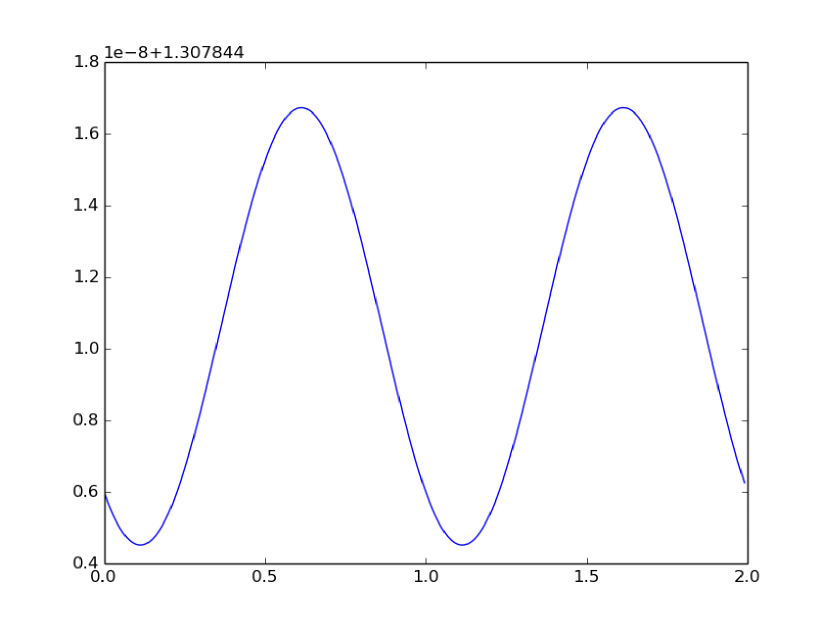
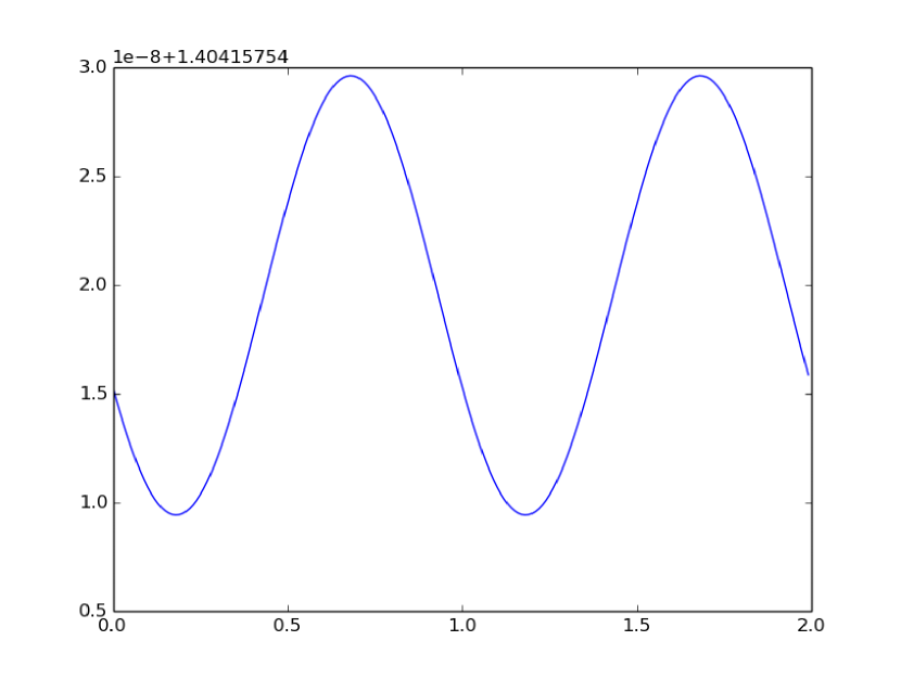
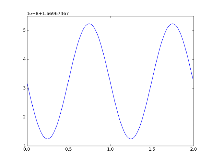
Figure 1: Plots of $H(\rho,x)$ for $\rho=-0.5,0,0.5$.

Again, the depth exhibits a phase transition: for $p=1/2$ we have $D_{n}/\log n\to 1/\log 2$ almost surely, which doesn’t hold for $p>1/2$. We note that some of the results on the depth (namely, the convergence in probability and the central limit theorem) are already known (see [20]), but our contribution is a novel derivation of these facts via the profile analysis. Qualitatively, the oscillatory behavior of the external profile that is responsible for the lack of local limit theorem for the depth occurs also in both tries and digital search trees.

We now explain our approach to the analysis of the moments of $B_{n,k}$ in appropriate ranges (we follow [13, 15]). For this, we take an analytic approach [8, 23]. We first explain it for the analysis relevant to $D_{n}$, and then show how to extend it for $H_{n}$ and $F_{n}$. More details can be found in the next section.

We start by deriving a recurrence for the average profile, which we denote by $\mu_{n,k}:={\mathbb{E}}[B_{n,k}]$. It satisfies

$$\mu_{n,k}=(p^{n}+q^{n})\mu_{n,k}+\sum_{j=1}^{n-1}{n\choose j}p^{j}q^{n-j}(\mu_{j,k-1}+\mu_{n-j,k-1})$$ (6)

for $n\geq 2$ and $k\geq 1$, with some initial/boundary conditions; most importantly, $\mu_{n,k}=0$ for $k\geq n$ and any $n$. Moreover, $\mu_{n,k}\leq n$ for all $n$ and $k$ owing to the elimination of inconclusive queries. This recurrence arises from conditioning on the number $j$ of objects that are included in the first query. If $1\leq j\leq n-1$ objects are included, then the conditional expectation is a sum of contributions from those objects that are included and those that aren’t. If, on the other hand, all objects are included or all are excluded from the first potential query (which happens with probability $p^{n}+q^{n}$), then the partition element splitting constraint on the queries applies, the potential query is ignored as inconclusive, and the contribution is $\mu_{n,k}$.

The tools that we use to solve this recurrence (for details see [13, 15]) are similar to those of the analyses for digital trees [23] such as tries and digital search trees (though the analytical details differ significantly). We first derive a functional equation for the Poisson transform $\tilde{G}_{k}(z)=\sum_{m\geq 0}\mu_{m,k}\frac{z^{m}}{m!}e^{-z}$ of $\mu_{n,k}$, which gives

$$\tilde{G}_{k}(z)=\tilde{G}_{k-1}(pz)+\tilde{G}_{k-1}(qz)+e^{-pz}(\tilde{G}_{k}-\tilde{G}_{k-1})(qz)+e^{-qz}(\tilde{G}_{k}-\tilde{G}_{k-1})(pz).$$

This we write as

$$\tilde{G}_{k}(z)=\tilde{G}_{k-1}(pz)+\tilde{G}_{k-1}(qz)+\tilde{W}_{k,G}(z),$$ (7)

We contrast this functional equation with those for tries [16] and for digital search trees [6]: in tries, the expression $\tilde{W}_{k,G}(z)$ does not appear, which significantly simplifies the analysis in that case. In digital search trees, the functional equation is a differential equation, and the analysis is consequently quite different.

At this point the goal is to determine asymptotics for $\tilde{G}_{k}(z)$ as $z\to\infty$ in a cone around the positive real axis. When solving (7), $\tilde{W}_{k,G}(z)$ complicates the analysis because it has no closed-form Mellin transform (see below); we handle it via its Taylor series. Finally, depoissonization [23] will allow us to transfer the asymptotic expansion for $\tilde{G}_{k}(z)$ back to one for $\mu_{n,k}$:

$$\mu_{n,k}=\tilde{G}_{k}(n)-\frac{n}{2}\tilde{G}^{\prime\prime}_{k}(n)+O(n^{\epsilon-1}).$$

To convert (7) to an algebraic equation, we use the Mellin transform [7], which, for a function $f:{\mathbb{R}}\to{\mathbb{R}}$ is given by

$${f^{*}}(s)=\int_{0}^{\infty}z^{s-1}f(z){\;\mathrm{d}z}.$$

Using the Mellin transform identities and defining $T(s)=p^{-s}+q^{-s}$, we end up with an expression for the Mellin transform ${G_{k}^{*}}(s)$ of $\tilde{G}_{k}(z)$ of the form

$${G_{k}^{*}}(s)=\Gamma(s+1)A_{k}(s)(p^{-s}+q^{-s})^{k}=\Gamma(s+1)A_{k}(s)T(s)^{k},$$

where $A_{k}(s)$ (see (14) below) is an infinite series arising from the contributions coming from the function $\tilde{W}_{k,G}(z)$:

$$A_{k}(s)=\sum_{j=0}^{k}T(s)^{-j}\sum_{m=j}^{\infty}T(-m)(\mu_{m,j}-\mu_{m,j-1})\frac{\Gamma(m+s)}{\Gamma(m+1)\Gamma(s+1)},$$ (8)

where we define $\mu_{m,-1}=0$ for all $m$. Note that it involves $\mu_{m,j}-\mu_{m,j-1}$ for various $m$ and $j$ (see [13, 14]). Locating and characterizing the singularities of ${G_{k}^{*}}(s)$ then becomes important. We find that, for any $k$, $A_{k}(s)$ is entire, with zeros at $s\in{\mathbb{Z}}\cap[-k,-1]$, so that ${G_{k}^{*}}(s)$ is meromorphic, with possible simple poles at the negative integers less than $-k$. The fundamental strip of $\tilde{G}_{k}(z)$ then contains $(-k-1,\infty)$. It turns out that the main asymptotic contribution comes from an infinite number of saddle points (see (10) below) defined by the kernel $T(s)=p^{-s}+q^{-s}$.

We then must asymptotically invert the Mellin transform to recover $\tilde{G}_{k}(z)$. The Mellin inversion formula for ${G_{k}^{*}}(s)$ is given by

$$\tilde{G}_{k}(z)=\frac{1}{2\pi i}\int_{\rho-i\infty}^{\rho+i\infty}z^{-s}{G_{k}^{*}}(s){\;\mathrm{d}s}=\frac{1}{2\pi i}\int_{\rho-i\infty}^{\rho+i\infty}z^{-s}\Gamma(s+1)A_{k}(s)T(s)^{k}{\;\mathrm{d}s},$$ (9)

where $\rho$ is any real number inside the fundamental strip associated with $\tilde{G}_{k}(z)$. For $k$ in the range in which the profile grows polynomially (that coincides with the range of interest in our analysis of $D_{n}$), we evaluate this integral via the saddle point method [8]. Examining $z^{-s}T(s)^{k}$ and solving the associated saddle point equation

$$\frac{{\;\mathrm{d}}}{{\;\mathrm{d}s}}[k\log T(s)-s\log z]=0,$$

we find an explicit formula (12) below for $\rho(\alpha)$, the real-valued saddle point of our integrand. The multivaluedness of the complex logarithm then implies that there are infinitely many regularly spaced saddle points $s_{j}$, $j\in{\mathbb{Z}}$, on this vertical line:

$$s_{j}=\rho(\alpha)+i\frac{2\pi j}{\log(p/q)}.$$ (10)

These lead directly to oscillations in the $\Theta(1)$ factor in the final asymptotics for $\mu_{n,k}$). The main challenge in completing the saddle point analysis is then to elucidate the behavior of $\Gamma(s+1)A_{k}(s)$ for $s\to\infty$ along vertical lines: it turns out that this function inherits the exponential decay of $\Gamma(s+1)$ along vertical lines, and we prove it by splitting the sum defining $A_{k}(s)$ into two pieces, which decay exponentially for different reasons (the first sum decays as a result of the superexponential decay of $\mu_{m,j}$ for $m=\Theta(j)$, which is outside the main range of interest). We end up with an asymptotic expansion for $\tilde{G}_{k}(z)$ as $z\to\infty$ in terms of $A_{k}(s)$.

Finally, we must analyze the convergence properties of $A_{k}(s)$ as $k\to\infty$. We find that it converges uniformly on compact sets to a function $A(s)$ (see (14)) which is, because of the uniformity, entire. We then apply Lebesgue’s dominated convergence theorem to conclude that we can replace $A_{k}(s)$ with $A(s)$ in the final asymptotic expansion of $\tilde{G}_{k}(z)$. All of this yields the following theorem which is proved in [13, 15].

Theorem 3 (Moments and limiting distribution for $B_{n,k}$ for $k$ in the central region).

Let $\epsilon>0$ be independent of $n$ and $k$, and fix $\alpha\in\left(\frac{1}{\log(1/q)}+\epsilon,\frac{1}{\log(1/p)}-\epsilon\right)$. Then for $k=k_{\alpha,n}\sim\alpha\log n$:

(i) The expected external profile becomes

$${\mathbb{E}}[B_{n,k}] =H(\rho(\alpha),\log_{p/q}(p^{k}n))\cdot\frac{n^{\beta(\alpha)}}{\sqrt{2\pi\kappa_{*}(\rho(\alpha))\alpha\log n}}\left(1+O(\sqrt{\log n})\right),$$ (11)

where

$$\rho(\alpha)=-\frac{1}{\log(p/q)}\log\left(\frac{\alpha\log(1/q)-1}{1-\alpha\log(1/p)}\right), \beta(\alpha)=\alpha\log(T(\rho(\alpha)))-\rho(\alpha),$$ (12)

and $\kappa_{*}(\rho)$ is an explicitly known function of $\rho$. Furthermore, $H(\rho,x)$ (see Figure 1) is a non-zero periodic function with period $1$ in $x$ given by

$$H(\rho,x)=\sum_{j\in{\mathbb{Z}}}A(\rho+it_{j})\Gamma(\rho+1+it_{j})e^{-2j\pi ix},$$ (13)

where $t_{j}=2\pi j/\log(p/q)$, and

$$A(s)=\sum_{j=0}^{\infty}T(s)^{-j}\sum_{n=j}^{\infty}T(-n)(\mu_{n,j}-\mu_{n,j-1})\frac{\phi_{n}(s)}{n!},$$ (14)

where $\phi_{n}(s)=\prod_{j=1}^{n-1}(s+j)$ for $n>1$ and $\phi_{n}(s)=1$ for $n\leq 1$. We recall that $T(s)=p^{-s}+q^{-s}$. Here, $A(s)$ is an entire function which is zero at the negative integers.

(ii) The variance of the profile is ${\mathrm{Var}}[B_{n,k}]=\Theta({\mathbb{E}}[B_{n,k}]).$

(iii) The limiting distribution of the normalized profile is Gaussian; that is,

$$\frac{B_{n,k}-\mu_{n,k}}{\sqrt{{\mathrm{Var}}[B_{n,k}]}}\xrightarrow{D}{\mathcal{N}}(0,1)$$

where ${\mathcal{N}}(0,1)$ is the standard normal distribution.

We should point out that the unusual behavior of $D_{n}$ in Rényi’s problem is a direct consequence of the oscillatory behavior of the profile, which disappears for the symmetric case. Furthermore, for the height and fillup level analyses we need to extend Theorem 3 beyond its original central range for $\alpha$, as discussed in the next section.

3 Proof sketches

Now we give sketches of the proofs of Theorems 1 and 2 with more details regarding the proof of Theorem 1 in the forthcoming journal version [5]. In particular, in this conference version, we only sketch derivations for $H_{n}$ and for $F_{n}$ by upper and lower bounding, respectively. As stated earlier, the proof of Theorem 3 can be found in [13, 15].

3.1 Sketch of the proof of Theorem 1

To prove our results for $H_{n}$ and $F_{n}$, we extend the analysis of $B_{n,k}$ to the boundaries of the central region (i.e., $k\sim\log_{1/p}n$ and $k\sim\log_{1/q}n$).

Derivation of $H_{n}$. Fixing any $\epsilon>0$, we write, for the lower bound on the height,

$$k_{L}=\log_{1/p}n+(1-\epsilon)\psi(n)$$

and, for the upper bound,

$$k_{U}=\log_{1/p}n+(1+\epsilon)\psi(n),$$

for a function $\psi(n)=o(\log n)$ which we are to determine. In order for the first and second moment methods to work, we require $\mu_{n,k_{L}}\xrightarrow{n\to\infty}\infty$ and $\mu_{n,k_{U}}\xrightarrow{n\to\infty}0.$ (We additionally need that ${\mathrm{Var}}[B_{n,k_{L}}]=o(\mu_{n,k_{L}}^{2})$, but this is not too hard to show by induction using the recurrence for $\tilde{V}_{k}(z)$, the Poisson variance of $B_{n,k}$.) In order to identify the $\psi(n)$ at which this transition occurs, we define $k=\log_{1/p}n+\psi(n)$, and the plan is to estimate ${\mathbb{E}}[B_{n,k}]$ via the integral representation (9) for its Poisson transform. Specifically, we consider the inverse Mellin integrand for some $s=\rho\in{\mathbb{Z}}^{-}+1/2$ to be set later. This is sufficient for the upper bound, since, by the exponential decay of the $\Gamma$ function, the entire integral is at most of the same order of growth as the integrand on the real axis. We expand the integrand in (9), that is,

$$J_{k}(n,s):=\sum_{j=0}^{k}n^{-s}T(s)^{k-j}\sum_{m\geq j}T(-m)(\mu_{m,j}-\mu_{m,j-1})\frac{\Gamma(m+s)}{\Gamma(m+1)},$$ (15)

and apply a simple extension of Theorem 2.2, part (iii) of [14] to approximate $\mu_{m,j}-\mu_{m,j-1}$ when $j\to\infty$ and is close enough to $m$:

Lemma 2 (Precise asymptotics for $\mu_{n,k}$, $k\to\infty$ and $n$ near $k$).

Let $p\geq q$. For $n\to\infty$ with $1\leq k<n$ and $\log^{2}(n-k)=o(k)$,

$$\mu_{n,k}\sim(n-k)^{3/2+\frac{\log q}{\log p}}\frac{n!}{(n-k)!}p^{k^{2}/2+k/2}q^{k}\cdot\exp\left(-\frac{\log^{2}(n-k)}{2\log(1/p)}\right)\Theta(1).$$ (16)

Moreover, for $n\to\infty$ and $k<n$, for some constant $C>0$,

$$\mu_{n,k}\leq C\frac{n!}{(n-k-1)!}p^{k^{2}/2+k/2+O(log(n-k)^{2})}q^{k}.$$

Now, we continue with the evaluation of (15). The $j$th term of (15) is then of order $p^{\nu_{j}(n,s)},$ where we set

$$\nu_{j}(n,s)=~{} (j-\psi(n))^{2}/2+(j-\psi(n))(s+\log_{1/p}(1+(p/q)^{s})+\psi(n)+1)$$

$$-\log_{1/p}n\log_{1/p}(1+(p/q)^{s})+\psi(n)^{2}/2+o(\psi(n)^{2}).$$

The factor $T(s)^{k-j}$ ensures that the bounded $j$ terms are negligible.

Our next goal is to find the $j$ which gives the dominant contribution to the sum in (15); that is, the $j$ for which the contributions $p^{\nu_{j}(n,s)}$ dominate. By elementary calculus, we can find the $j$ term which minimizes $\nu_{j}(n,s)$:

$$j=-(s+\log_{1/p}(1+(p/q)^{s})+1).$$

Then $\nu_{j}(n,s)$ for this value of $j$ becomes

$$\nu_{j}(n,s) =-\frac{(s+\log_{1/p}(1+(p/q)^{s})+\psi(n)+1)^{2}}{2}$$

$$~{}~{}~{}~{}-\log_{1/p}n\log_{1/p}(1+(p/q)^{s})+\psi(n)^{2}/2+o(\psi(n)^{2}).$$ (17)

We then minimize over all $s$, which requires us to split into the symmetric and asymmetric cases.

Symmetric case:

When $p=q=1/2$, we have $\log_{1/p}(1+(p/q)^{s})=\log_{2}(2)=1$, so that the expression for $\nu_{j}(n,s)$ simplifies, and we get $s=-\psi(n)+O(1)$. The optimal value for $\nu_{j}(n,s)$ then becomes

$$\nu_{j}(n,s)=-\log_{2}n+\psi(n)^{2}/2+o(\psi(n)^{2}).$$ (18)

We have thus succeeded in finding a likely candidate for the range of $j$ terms that contribute maximally, as well as an upper bound on their contribution. This gives a tight upper bound on $J_{k}(n,s)$ and, hence, on $\tilde{G}_{k}(n)$, of $\Theta(2^{-\nu_{j}(n,s)})$.

Now, to find $\psi(n)$ for which there is a phase transition in this bound from tending to $\infty$ to tending to $0$, we set the exponent in the above expression equal to zero and solve for $\psi(n)$. This gives

$$-\log_{2}n+\psi(n)^{2}/2(1+o(1))=0\implies\psi(n)\sim\sqrt{2\log_{2}n},$$

as expected.

Asymmetric case:

On the other hand, when $p>1/2$, the equation that we need to solve to find the minimizing value of $s$ for (17) is a bit more complicated, owing to the fact that $\log_{1/p}(1+(p/q)^{s})$ now depends on $s$: taking a derivative with respect to $s$ in (17) and setting this equal to $0$, after some algebra, we must solve

$$-\frac{(p/q)^{s}\log(p/q)}{\log(1/p)}\log_{1/p}n-\psi(n)(1+O((p/q)^{s}))-s(1+O((p/q)^{s}))+O((p/q)^{s})=0$$ (19)

for $s$. Here, we note that we used the approximation

$$\log_{1/p}(1+(p/q)^{s})=\frac{(p/q)^{s}}{\log(1/p)}+O((p/q)^{2}),$$

which is valid since we are looking for $s\to-\infty$.

To find a solution to (19), we first note that it implies that $s<-\psi(n)$ (since the first term involving $\log n$ is negative), and, if $\psi(n)>0$, this implies that

$$-\psi(n)-s=-O(s).$$ (20)

The plan, then, is to use this to guess a solution $s$ for (19), which we can then verify. The equality (20) suggests that we replace $-\psi(n)-s+O((p/q)^{s})$ with $-C\cdot s$ in (19), for some constant $C>0$. Then the equation becomes

$$-Cs-\frac{(p/q)^{s}\log(p/q)}{\log(1/p)}\log_{1/p}n=0.$$

After some trivial rearrangement and multiplication of both sides by $\log(p/q)$, we get

$$-s\log(p/q)\cdot e^{-s\log(p/q)}=\Theta(\log n).$$

Setting $W=-s\log(p/q)$ brings us to an expression of the form that defines the Lambert $W$ function [1] (i.e., a function $W(z)$ satisfying $W(z)e^{W(z)}=z$).

Using the asymptotics of the $W$ function for large $z$ [1], we thus find that

$$s=-\log_{p/q}\log n+O(\log\log\log n).$$

Note that $s\to-\infty$, as required. This may be plugged into (17) to see that it is indeed a solution to the equation.

Now, to find the correct choice of $\psi(n)$ for which there is a phase transition, we plug this choice of $s$ into (17), set it equal to $0$, and solve for $\psi(n)$. This gives

$$\psi(n)=-\frac{s}{2}=\frac{1}{2}\log_{p/q}\log n+O(\log\log\log n),$$ (21)

as desired.

Note that replacing $\psi(n)$ in (17) with $(1+\epsilon)\psi(n)$ yields a maximum contribution to the inverse Mellin integral of

$$J_{k_{U}}(n,s)=O(p^{\frac{\epsilon}{2}(\log_{p/q}\log n)^{2}+o((\log\log n)^{2})})\to 0.$$ (22)

When we replace $\psi(n)$ with $(1-\epsilon)\psi(n)$, we get

$$J_{k_{L}}(n,s)=O(p^{-\frac{\epsilon}{2}(\log_{p/q}\log n)^{2}+o((\log\log n)^{2})}),$$ (23)

so that the upper bound tends to infinity (in [5], we prove a matching lower bound).

The above analysis gives asymptotic estimates for $\tilde{G}_{k}(n)$. We then apply analytic depoissonization [23] to get

$$\mu_{n,k}=\tilde{G}_{k}(n)-\frac{n}{2}\tilde{G}^{\prime\prime}_{k}(n)+O(n^{\epsilon-1}),$$

(where the second term can be handled in the same way as the first). This gives the claimed result.

Derivation of $F_{n}$. We now set $k=\log_{1/q}n+\psi(n)$ and

$$k_{L}=\log_{1/q}n+(1+\epsilon)\psi(n), k_{U}=\log_{1/q}n+(1-\epsilon)\psi(n).$$ (24)

Here, $\psi(n)=o(\log n)$ is to be determined so as to satisfy $\mu_{n,k_{L}}\to 0$ and $\mu_{n,k_{U}}\to\infty$. We use a technique similar to that used in the height proof to determine $\psi(n)$, except now the $\Gamma$ function asymptotics play a role, since we will choose $\rho\in{\mathbb{R}}$ tending to $\infty$. Our first task is to upper bound (as tightly as possible), for each $j$, the magnitude of the $j$th term of (15). First, we upper bound

$$T(-m)(\mu_{m,j}-\mu_{m,j-1})\leq 2p^{m}\mu_{m,j}\leq 2p^{m}m,$$ (25)

using the boundary conditions on $\mu_{m,j}$. Next, we apply Stirling’s formula to get

$$\frac{\Gamma(m+\rho)}{\Gamma(m+1)} \sim\sqrt{1+\rho/m}\left(\frac{m+\rho}{e}\right)^{m+\rho}\left(\frac{m+1}{e}\right)^{-(m+1)}$$ (26)

$$=e^{(m+\rho)\log(m+\rho)-(m+\rho)+m+1-(m+1)\log(m+1)+O(\log\rho)}$$ (27)

$$=\exp((m+\rho)\log(m+\rho)-(m+1)\log(m+1)+O(\rho))$$ (28)

$$=\exp(m\log(m(1+\rho/m))+\rho\log(\rho(1+m/\rho))-m\log m-\log m+O(\rho))$$ (29)

$$=\exp(m\log(1+\rho/m)+\rho\log(\rho)+\rho\log(1+m/\rho)-\log m+O(\rho)).$$ (30)

Multiplying (25) and (30), then optimizing over all $m\geq j$, we find that the maximum term of the $m$ sum occurs at $m=\rho p/q$ and has a value of

$$\exp(\rho\log\rho+O(\rho)).$$ (31)

Now, observe that when $\log m\gg\log\rho$, the contribution of the $m$th term is $p^{m+o(m)}=e^{-\Theta(m)}$. Thus, setting $j^{\prime}=\rho^{\log\rho}$ (note that $\log j^{\prime}=(\log\rho)^{2}\gg\log\rho$), we split the $m$ sum into two parts:

$$\sum_{m\geq j}2p^{m}m\frac{\Gamma(m+\rho)}{\Gamma(m+1)}=\sum_{m=j}^{j^{\prime}}2p^{m}m\frac{\Gamma(m+\rho)}{\Gamma(m+1)}+\sum_{m=j^{\prime}+1}^{\infty}2p^{m}m\frac{\Gamma(m+\rho)}{\Gamma(m+1)}.$$

The terms of the initial part can be upper bounded by (31), while those of the final part are upper bounded by $e^{-\Theta(m)}$ (so that the final part is the tail of a geometric series). This gives an upper bound of

$$j^{\prime}e^{\rho\log\rho+O(\rho)}+e^{-\Theta(j^{\prime})}=e^{(\log\rho)^{2}+\rho\log\rho+O(\rho)}=e^{\rho\log\rho+O(\rho)},$$

which holds for any $j$.

Multiplying this by $n^{-\rho}T(\rho)^{k-j}=q^{\rho\cdot(j-\psi(n))+(j-\psi(n)-\log_{1/q}n)\log_{1/q}(1+(q/p)^{\rho})}$ gives

$$q^{\rho(j-\psi(n))+(j-\psi(n)-\log_{1/q}n)\log_{1/q}(1+(q/p)^{\rho})-\rho\log_{1/q}\rho+O(\rho)}.$$ (32)

Maximizing over the $j$ terms, we find that the largest contribution comes from $j=0$. Then, just as in the height upper bound, the behavior with respect to $\rho$ depends on whether or not $p=q$, because $\log_{1/q}(1+(q/p)^{\rho})=1$ when $p=q$ and is dependent on $\rho$ otherwise. Taking this into account and minimizing over $\rho$ gives that the maximum contribution to the $j$ sum is minimized by setting $\rho=2^{-\psi(n)-\frac{1}{\log 2}}$ when $p=q$ and $\rho\sim\log_{p/q}\log n$ otherwise. Plugging these choices for $\rho$ into the exponent of (32), setting it equal to $0$, and solving for $\psi(n)$ gives $\psi(n)=-\log_{2}\log n+O(1)$ when $p=q$ and $\psi(n)\sim-\log_{1/q}\log\log n$ when $p>q$. The evaluation of the inverse Mellin integral with $k=k_{L}$ as defined in (24) and the integration contour given by $\Re(s)=\rho$ proceeds along lines similar to the height proof, and this yields the desired result.

We remark that the lower bound for $F_{n}$ may also be derived by relating it to the analogous quantity in regular tries: by definition of the fillup level, there are no unary paths above the fillup level in a standard trie. Thus, when converting the corresponding PATRICIA trie, no path compression occurs above this level, which implies that $F_{n}$ for PATRICIA is lower bounded by that of tries (and the typical value for tries is the same as in our theorem for PATRICIA). We include the lower bound for $F_{n}$ via the bounding of the inverse Mellin integral because it is similar in flavor to the corresponding proof of the upper bound (for which no short proof seems to exist).

The upper bound for $F_{n}$ can similarly be handled by an exact evaluation of the inverse Mellin transform.

3.2 Proof of Theorem 2

Using Theorem 3, we can prove Theorem 2.

Convergence in probability: For the typical value of $D_{n}$, we show that

$$\Pr[D_{n}<(1-\epsilon)\frac{1}{h(p)}\log n]\xrightarrow{n\to\infty}0, \Pr[D_{n}>(1+\epsilon)\frac{1}{h(p)}\log n]\xrightarrow{n\to\infty}0.$$ (33)

For the lower bound, we have

$$\Pr[D_{n}<(1-\epsilon)\frac{1}{h(p)}\log n]=\sum_{k=0}^{\lfloor{(1-\epsilon)\frac{1}{h(p)}\log n}\rfloor}\Pr[D_{n}=k]=\sum_{k=0}^{\lfloor{(1-\epsilon)\frac{1}{h(p)}\log n}\rfloor}\frac{\mu_{n,k}}{n}.$$

We know from Theorem 3 and the analysis of $F_{n}$ that, in the range of this sum, $\mu_{n,k}=O(n^{1-\epsilon})$. Plugging this in, we get

$$\Pr[D_{n}<(1-\epsilon)\frac{1}{h(p)}\log n]=\sum_{k=0}^{\lfloor{(1-\epsilon)\frac{1}{h(p)}\log n}\rfloor}O(n^{-\epsilon})=O(n^{-\epsilon}\log n)=o(1).$$

The proof for the upper bound is very similar, except that we appeal to the analysis of $H_{n}$ instead of $F_{n}$.

No almost sure convergence: To show that $D_{n}/\log n$ does not converge almost surely, we show that

$$\liminf_{n\to\infty}D_{n}/\log n=1/\log(1/q), \limsup_{n\to\infty}D_{n}/\log n=1/\log(1/p).$$ (34)

For this, we first show that, almost surely, $F_{n}/\log n\xrightarrow{n\to\infty}1/\log(1/q)$ and $H_{n}/\log n\xrightarrow{n\to\infty}1/\log(1/p)$. Knowing this, we consider the following sequences of events: $A_{n}$ is the event that $D_{n}=F_{n}+1$, and $A^{\prime}_{n}$ is the event that $D_{n}=H_{n}$. We note that all elements of the sequences are independent, and $\Pr[A_{n}],\Pr[A^{\prime}_{n}]\geq 1/n$. This implies that $\sum_{n=1}^{\infty}\Pr[A_{n}]=\sum_{n=1}^{\infty}\Pr[A^{\prime}_{n}]=\infty$, so that the Borel-Cantelli lemma tells us that both $A_{n}$ and $A^{\prime}_{n}$ occur infinitely often almost surely (moreover, $F_{n}<D_{n}\leq H_{n}$ by definition of the relevant quantities). This proves (34).

To show the claimed almost sure convergence of $F_{n}/\log n$ and $H_{n}/\log n$, we cannot apply the Borel-Cantelli lemmas directly, because the relevant sums do not converge. Instead, we apply a trick which was used in [17]. We observe that both $(F_{n})$ and $(H_{n})$ are non-decreasing sequences. Next, we show that, on some appropriately chosen subsequence, both of these sequences, when divided by $\log n$, converge almost surely to their respective limits. Combining this with the observed monotonicity yields the claimed almost sure convergence, and, hence, the equalities in (34).

We illustrate this idea more precisely for $H_{n}$. By our analysis above, we know that

$$\Pr[|H_{n}/\log n-1/\log(1/p)|>\epsilon]=O(e^{-\Theta(\log\log n)^{2}}).$$

Then we fix $t$, and we define $n_{r,t}=2^{t^{2}2^{2r}}$. On this subsequence, by the probability bound just stated, we can apply the Borel-Cantelli lemma to conclude that $H_{n_{r,t}}/\log(n_{r,t})\xrightarrow{r\to\infty}1/\log(1/p)\cdot(t+1)^{2}/t^{2}$ almost surely. Moreover, for every $n$, we can choose $r$ such that $n_{r,t}\leq n\leq n_{r,t+1}$. Then

$$H_{n}/\log n\leq H_{n_{r,t+1}}/\log n_{r,t},$$

which implies

$$\limsup_{n\to\infty}\frac{H_{n}}{\log n}\leq\limsup_{r\to\infty}\frac{H_{n_{r,t+1}}}{\log n_{r,t+1}}\frac{\log n_{r,t+1}}{\log n_{r,t}}=\frac{1}{\log(1/p)}\cdot\frac{(t+1)^{2}}{t^{2}}.$$

Taking $t\to\infty$, this becomes $1/\log(1/p)$, as desired. The argument for the $\liminf$ is similar, and this establishes the almost sure convergence of $H_{n}$. The derivation is entirely similar for $F_{n}$.

Asymptotics for probability mass function of $D_{n}$: The asymptotic formula for $\Pr[D_{n}=k]$ with $k$ as in the theorem follows directly from the fact that $\Pr[D_{n}=k]={\mathbb{E}}[B_{n,k}]/n$, plugging in the expression of Theorem 3 for ${\mathbb{E}}[B_{n,k}]$.

References

- [1] Milton Abramowitz and Irene A. Stegun. Handbook of Mathematical Functions with Formulas, Graphs, and Mathematical Tables, volume 55 of National Bureau of Standards Applied Mathematics Series. For sale by the Superintendent of Documents, U.S. Government Printing Office, Washington, D.C., 1964.
- [2] Luc Devroye. A note on the probabilistic analysis of patricia trees. Random Struct. Algorithms, 3(2):203–214, March 1992.
- [3] Luc Devroye. Laws of large numbers and tail inequalities for random tries and patricia trees. Journal of Computational and Applied Mathematics, 142:27–37, 2002.
- [4] Luc Devroye. Universal asymptotics for random tries and patricia trees. Algorithmica, 42(1):11–29, 2005.
- [5] Michael Drmota, Abram Magner, and Wojciech Szpankowski. Asymmetric Rényi problem and PATRICIA tries. In preparation.
- [6] Michael Drmota and Wojciech Szpankowski. The expected profile of digital search trees. J. Comb. Theory Ser. A, 118(7):1939–1965, October 2011.
- [7] Philippe Flajolet, Xavier Gourdon, and Philippe Dumas. Mellin transforms and asymptotics: Harmonic sums. Theoretical Computer Science, 144:3–58, 1995.
- [8] Philippe Flajolet and Robert Sedgewick. Analytic Combinatorics. Cambridge University Press, Cambridge, UK, 2009.
- [9] Svante Janson and Wojciech Szpankowski. Analysis of an asymmetric leader election algorithm. Electronic J. Combin, 4:1–6, 1996.
- [10] Ramin Kazemi and Mohammad Vahidi-Asl. The variance of the profile in digital search trees. Discrete Mathematics and Theoretical Computer Science, 13(3):21–38, 2011.
- [11] Philippe Jacquet, Charles Knessl, and Wojciech Szpankowski. A note on a problem posed by D. E. Knuth on a satisfiability recurrence. Combinatorics, Probability, and Computing, 23, 839-841, 2014.
- [12] Donald E. Knuth. The Art of Computer Programming, Volume 3: (2nd ed.) Sorting and Searching. Addison Wesley Longman Publishing Co., Inc., Redwood City, CA, USA, 1998.
- [13] Abram Magner. Profiles of PATRICIA Tries. PhD thesis, Purdue University, December 2015.
- [14] Abram Magner, Charles Knessl, and Wojciech Szpankowski. Expected external profile of patricia tries. Proceedings of the Eleventh Workshop on Analytic Algorithmics and Combinatorics, pages 16–24, 2014.
- [15] Abram Magner and Wojciech Szpankowski. Profile of PATRICIA tries. submitted. http://www.cs.purdue.edu/~spa/papers/patricia2015.pdf
- [16] G. Park, H. Hwang, P. Nicodème, and W. Szpankowski. Profiles of tries. SIAM Journal on Computing, 38(5):1821–1880, 2009.
- [17] B. Pittel. Asymptotic growth of a class of random trees. Ann. Probab., 18:414–427, 1985.
- [18] B. Pittel, Paths in a random digital tree: limiting distributions, Adv. in Applied Probability, 18, 139–155, 1986.
- [19] Boris Pittel and Herman Rubin. How many random questions are needed to identify distinct objects? Journal of Combinatorial Theory, Series A, 55(2):292–312, 1990.
- [20] B. Rais, P. Jacquet, and W. Szpankowski. Limiting distribution for the depth in PATRICIA tries. SIAM Journal on Discrete Mathematics, 6(2):197–213, 1993.
- [21] A. Rényi, On Random Subsets of a Finite Set, Mathematica, 3, 355-362, 1961.
- [22] Wojciech Szpankowski. Patricia tries again revisited. J. ACM, 37(4):691–711, October 1990.
- [23] Wojciech Szpankowski. Average Case Analysis of Algorithms on Sequences. John Wiley & Sons, Inc., New York, NY, USA, 2001.