Algorithms for Overcoming the Curse of Dimensionality for Certain Hamilton-Jacobi Equations Arising in Control Theory and Elsewhere

Abstract.

It is well known that time dependent Hamilton-Jacobi-Isaacs partial differential equations (HJ PDE), play an important role in analyzing continuous dynamic games and control theory problems. An important tool for such problems when they involve geometric motion is the level set method, [41]. This was first used for reachability problems in [36],[37]. The cost of these algorithms, and, in fact, all PDE numerical approximations is exponential in the space dimension and time.

In [13], some connections between HJ-PDE and convex optimization in many dimensions are presented. In this work we propose and test methods for solving a large class of the HJ PDE relevant to optimal control problems without the use of grids or numerical approximations. Rather we use the classical Hopf formulas for solving initial value problems for HJ PDE [30]. We have noticed that if the Hamiltonian is convex and positively homogeneous of degree one (which the latter is for all geometrically based level set motion and control and differential game problems) that very fast methods exist to solve the resulting optimization problem. This is very much related to fast methods for solving problems in compressive sensing, based on $\ell_{1}$ optimization [24],[51]. We seem to obtain methods which are polynomial in the dimension. Our algorithm is very fast, requires very low memory and is totally parallelizable. We can evaluate the solution and its gradient in very high dimensions at $10^{-4}$ to $10^{-8}$ seconds per evaluation on a laptop.

We carefully explain how to compute numerically the optimal control from the numerical solution of the associated initial valued HJ-PDE for a class of optimal control problems. We show that our algorithms compute all the quantities we need to obtain easily the controller.

In addition, as a step often needed in this procedure, we have developed a new and equally fast way to find, in very high dimensions, the closest point $y$ lying in the union of a finite number of compact convex sets $\Omega$ to any point $x$ exterior to the $\Omega$. We can also compute the distance to these sets much faster than Dijkstra type “fast methods ”, e.g. [15].

The term “curse of dimensionality”, was coined by Richard Bellman in 1957, [3][4], when considering problems in dynamic optimization. Keywords: Hamilton-Jacobi equation, Curse of dimensionaly, Hopf-Lax formula, Convex analysis, Convex optimization, Optimization Algorithms. 2010 Mathematics Subject Classification: 35F21, 46N10

1. Introduction to Hopf Formulas, HJ PDEs and Level Set Evolutions

We briefly introduce Hamilton-Jacobi equations with initial data and the Hopf formulas to represent the solution. We give some examples to show the potential of our approach, including examples to perform level set evolutions.

Given a continuous function $H:\mathbb{R}^{n}\rightarrow\mathbb{R}$ bounded from below by an affine function, we consider the HJ PDE

(1) $$\frac{\partial\varphi}{\partial t}(x,t)+H(\nabla_{x}\varphi(x,t))\;=\;0\quad\text{in }\mathbb{R}^{n}\times(0,+\infty),$$

where $\frac{\partial\varphi}{\partial t}$ and $\nabla_{x}\varphi$ respectively denote the partial derivative with respect to $t$ and the gradient vector with respect to $x$ of the function $\varphi$. We are also given some initial data

(2) $$\varphi(x,0)\;=\;J(x) \quad\forall\,x\in\mathbb{R}^{n},$$

where $J:\mathbb{R}^{n}\to\mathbb{R}$ is convex. For the sake of simplicity we only consider functions $\varphi$ and $J$ that are finite everywhere. Results presented in this paper can be generalized for $H:\mathbb{R}^{n}\to\mathbb{R}\cup\{+\infty\}$ and $J:\mathbb{R}^{n}\to\mathbb{R}\cup\{+\infty\}$ under suitable assumptions. We also extend our results to an interesting class of nonconvex initial data in section 2.2.

We wish to compute the viscosity solution [12],[11] for a given $x\in\mathbb{R}^{n}$ and $t>0$.

Using numerical approximations is essentially impossible for $n\geq 4$. The complexity of a finite difference equation is exponential in $n$ because the number of grid points is also exponential in $n$. This has been found to be impossible, even with the use of sophisticated e.g. ENO, WENO, DG, methods [42],[31],[52]. High order accuracy is no cure for this curse of dimensionality.

We propose and test a new approach, borrowing ideas from convex optimization, which arise in the $\ell_{1}$ regularization convex optimization [24],[51] used in compressive sensing [6],[17]. It has been shown experimentally that these $\ell_{1}$ based methods converge quickly when we use Bregman and split Bregman iterative methods. These are essentially the same as Augmented Lagrangian methods [25] and Alternating Direction Method of Multipliers methods [23]. These and related first order and splitting techniques have enjoyed a renaissance since they were recently used very successfully for these $\ell_{1}$ and related problems [51],[24]. One explanation for their rapid convergence is the “error forgetting” property discovered and analyzed in [43] for $\ell_{1}$ regularization.

We will solve the initial value problem (1)-(2) without discretization, using the Hopf formula [30]

(3) $$\varphi(x,t)\;=\; \left(J^{*}+tH\right)^{*}(x)$$

(4) $$\;=\; -\min_{v\in R^{n}}\left\{J^{*}(v)+tH(v)-\langle x,v\rangle\right\}$$

where the Fenchel-Legendre transform $f^{*}:\mathbb{R}^{n}\to\mathbb{R}\cup\{+\infty\}$ of a convex, proper, lower semicontinuous function $f:\mathbb{R}^{n}\to\mathbb{R}\cup\{+\infty\}$ is defined by [18, 28, 44]

(5) $$J^{*}(v)=\sup_{x\in R^{n}}\left\{\langle v,x\rangle-J(x)\right\},$$

where $\langle\cdot,\cdot\rangle$ denotes the $\ell_{2}(\mathbb{R}^{n})$ inner product. We also define for any $v\in\mathbb{R}^{n}$, $\|v\|_{p}=\left(\sum_{i=1}^{n}|v_{i}|^{p}\right)^{\frac{1}{p}}$ for $1\leq p<+\infty$ and $\|v\|_{\infty}=\max_{i=1,\dots,n}|v_{i}|$. Note that since $J:\mathbb{R}^{n}\to\mathbb{R}$ is convex we have that $J^{*}$ is 1-coercive [28, Prop. 1.3.9, p. 46], i.e., $\lim_{\|x\|\to+\infty}\frac{J^{*}(x)}{\|x\|_{2}}\;=\;+\infty$. When the gradient $\nabla_{x}\varphi(x,t)$ exists, then it is precisely the unique minimizer of (4); in addition, the gradient will also provide the optimal control considered in this paper (see Section 2) For instance, this holds for any $x\in\mathbb{R}^{n}$ and $t>0$ when $H:\mathbb{R}^{n}\to\mathbb{R}$ is convex, $J:\mathbb{R}^{n}\to\mathbb{R}$ is strictly convex, differentiable and 1-coercive. The Hopf formula only requires the convexity of $J$ and the continuity of $H$, but we will often require that $H$ in (1) is also convex.

We note that the case $H=\|\cdot\|_{1}$ corresponds to $H(\nabla_{x}\varphi(x,t))=\sum_{i=1}^{n}\left|\frac{\partial}{\partial x_{i}}\varphi(x,t)\right|$, used, e.g. to compute the Manhattan distance to the zero level set of $x\mapsto J(x)$, [15]. This optimization is closely related to the $\ell_{1}$ type minimization [6, 17],

$$\min_{v\in\mathbb{R}^{n}}\left\{\|v\|_{1}+\frac{\lambda}{2}\|Av-b\|_{2}^{2}\right\},$$

where $A$ is an $m\times n$ matrix with real entries, $m<n$, and $\lambda>0$ arising in compressive sensing. Let $\Omega\subset\mathbb{R}^{n}$ be a closed convex set. We denote by $\mbox{int }\Omega$ the interior of $\Omega$. If $J(x)<0$ for $x\in\mbox{int }\Omega$, $J(x)>0$ for $x\in(\mathbb{R}^{n}\setminus\Omega)$ and $J(x)=0$ for $x\in(\Omega\setminus\mbox{int }\Omega)$, then the solution $\varphi$ of (1)-(2) has the property that for any $t>0$ the set $\{x\in\mathbb{R}^{n}\;|\;\varphi(x,t)=0\}$ is precisely the set of points in $\mathbb{R}^{n}\setminus\Omega$ for which the Manhattan distance to $\Omega$ is equal to $t>0$. This is an example of the use of the level set method [41].

Similarly, if we take $H=\|\cdot\|_{2}$ then for any $t>0$ the resulting zero level set of $x\mapsto\varphi(x,t)$ will be the points in $\mathbb{R}^{n}\setminus\Omega$ whose Euclidean distance to $\Omega$ is equal to $t$. This fact will be useful later when we find the projection from a point $x\in\mathbb{R}^{n}$ to a compact, convex set $\Omega$.

We present here two somewhat simple but illustrative examples to show the potential power of our approach. Time results are presented in Section 4 and show that we can compute solution of some HJ-PDEs in fairly high dimensions at a rate below a millisecond per evaluation on a standard laptop.

Let $H=\|\cdot\|_{1}$ and $J(x)=\frac{1}{2}\left(\sum_{i=1}^{n}\frac{x_{i}^{2}}{a_{i}^{2}}-1\right)$ with $a_{i}>0$ for $i=1,\dots,n$. Then, for a given $t>0$, the set $\{x\in\mathbb{R}^{n}\;|\;\varphi(x,t)=0\}$ will be precisely the set of points at Manhattan distance $t$ outside of the ellipsoid determined by $\{x\in\mathbb{R}^{n}\;|\;J(x)\leq 0\}$. Following [28, Prop. 1.3.1, p. 42] it is easy to see that $J^{*}(x)\;=\;\frac{1}{2}\sum_{i=1}^{n}a_{i}^{2}x_{i}+\frac{1}{2}$. So:

$$\varphi(x,t)\;=\; -\frac{1}{2}-\min_{v\in R^{n}}\left\{\frac{1}{2}\sum_{i=1}^{n}a_{i}^{2}v_{i}^{2}+t\sum_{i=1}^{n}|v_{i}|-\langle x,v\rangle\right\}$$

$$\;=\; -\frac{1}{2}-\min_{v\in R^{n}}\left\{\frac{1}{2}\sum_{i=1}^{n}a_{i}^{2}\left(v_{i}-\frac{x_{i}}{a_{i}^{2}}\right)^{2}+t\sum_{i=1}^{n}|v_{i}|\right\}+\frac{1}{2}\sum_{i=1}^{n}\frac{x_{i}^{2}}{a_{i}^{2}}.$$

We note that the function to be minimized decouples into scalar minimizations of the form

$$\min_{y\in\mathbb{R}^{n}}\left(\frac{1}{2}\|y-x\|_{2}^{2}+\alpha\|y\|_{1}\right),\ \ \alpha>0.$$

The unique minimizer is the classical soft thresholding operator [33, 21, 14] defined for any component $i=1,\dots,n$ by

(6) $$\left(\mbox{shrink}_{1}(x,\alpha)\right)_{i}\;=\;\begin{dcases}x_{i}-\alpha&\mbox{ if }x_{i}>\alpha,\\ 0&\mbox{ if }|x_{i}|\leq\alpha,\\ x_{i}+\alpha&\mbox{ if }x_{i}<-\alpha.\end{dcases}$$

Therefore, for any $x\in\mathbb{R}^{n}$, any $t>0$ and any $i=1,\dots,n$ we have

$$\frac{\partial\varphi}{\partial x_{i}}(x,t)\;=\;\frac{1}{(a_{i})^{2}}\ \left(\mbox{shrink}_{1}(x,t)\right)_{i},$$

and

$$\varphi(x,t)=-\frac{1}{2}+\sum_{i\in\{0,\dots,n\}\setminus B(t)}\frac{1}{2}\left(\frac{|x_{i}|-t}{a_{i}}\right)^{2}.$$

Here $B(t)\subseteq\{0,\dots,n\}$ consists of indices for which $|x_{i}|\leq t$, and thus $\{0,\dots,n\}\setminus B(t)$ corresponds to indices for which $|x_{i}|>t$, and the zero level set moves outwards in this elegant fashion.

We note that in the above case we were able to compute the solution analytically and the dimension $n$ played no significant role. Of course this is rather a special problem, but this gives us some idea of what to expect in more complicated cases, discussed in section 3.

We will often need another shrink operator, i.e., when we solve the optimization problem with $\alpha>0$ and $x\in\mathbb{R}^{n}$

$$\min_{v\in\mathbb{R}^{n}}\left\{\frac{1}{2}\|v-x\|_{2}^{2}+\alpha\|v\|_{2}\right\}.$$

Its unique minimizer is given by

(7) $$\hbox{shrink}_{2}(x,\alpha)\;=\;\begin{cases}\frac{x}{\|x\|_{2}}\max(\|x\|_{2}-\alpha,0)&\mbox{ if }x\neq 0,\\ 0&\mbox{ if }x=0.\end{cases}$$

and thus its optimal value corresponds to the Huber function (see [50] for instance)

$$\min_{v\in\mathbb{R}^{n}}\left\{\frac{1}{2}\|v-x\|_{2}^{2}+\alpha\|v\|_{2}\right\}\;=\;\begin{cases}\frac{1}{2}\|x\|_{2}&\hbox{ if }\|x\|_{2}\leq\alpha,\\ \alpha\|x\|_{2}-\frac{\alpha^{2}}{2}&\hbox{ if }\|x\|_{2}>\alpha.\end{cases}$$

To move the unit sphere outwards with normal velocity 1, we use the following formula

$$\varphi(x,t) =-\min_{v\in\mathbb{R}^{n}}\left(\frac{\|v\|_{2}^{2}}{2}-t\|v\|_{2}-\langle x,v\rangle\right)-\frac{1}{2}$$

$$=-\min_{v\in\mathbb{R}^{n}}\left\{\frac{1}{2}\|v-x\|_{2}^{2}+t\|v\|_{2}\right\}+\frac{1}{2}(\|x\|_{2}^{2}-1)$$

$$=\begin{cases}\frac{1}{2}(\|x\|_{2}-t)^{2}-\frac{1}{2}&\mbox{ if }\|x\|_{2}>t\\ -\frac{1}{2}&\mbox{ if }\|x\|_{2}\leq t,\end{cases}$$

and, unsurprisingly, the zero level set of $x\mapsto\varphi(x,t)$ is the set $x$ satisfying $\|x\|_{2}=t+1$, for $t>0$.

These two examples will be generalized below so that we can, with extreme speed, compute the signed distance, either Euclidean, Manhattan or various generalizations, to the boundary of the union of a finite collection of compact convex sets.

The remainder of this paper is organized as follows: Section 2 contains an introduction to optimal control and its connection to HJ-PDE. Section 3 gives the details of our numerical methods. Section 4 presents numerical results with some details. We draw some concluding remarks and give future plans in Section 5. The appendix links our approach to the concepts of gauge and support functions in convex analysis.

2. Introduction to Optimal Control

First, we give a short introduction to optimal control and its connection to HJ PDE which is given in (11). We also introduce positively homogeneous of degree one Hamiltonians and describe their relationship to optimal control problems. We explain how to recover the optimal control from the solution of the HJ-PDE. An appendix describes further connections between these Hamiltonians and gauge in convex analysis. Second, we present some extensions of our work.

2.1. Optimal control and HJ-PDE

We are largely following the discussion in [16], see also [19], about optimal control and its link with HJ PDE. We briefly present it formally and we specialize it to the cases considered in this paper.

Suppose we are given a fixed terminal time $T\in\mathbb{R}$, an initial time $t<T$ along with an initial $x\in\mathbb{R}^{n}$. We consider the Lipschitz solution $x:[t,T]\to\mathbb{R}^{n}$ of the following ordinary differential equation

(9) $$\begin{cases}\frac{d\mathrm{x}}{ds}(s)\;=\;f\left(\beta(s)\right)&\mbox{ in }(t,T),\\ \mathrm{x}(t)\;=\;x,\end{cases}$$

where $f:C\to\mathbb{R}^{n}$ is a given bounded Lipschitz function and $C$ some given compact set of $\mathbb{R}^{n}$. The solution of (9) is affected by the measurable function $\beta:(-\infty,T]\to C$ which is called a control. We note $\mathcal{A}=\{\beta:(-\infty,T]\to C\;|\;\beta\mbox{ is measurable}\}$. We consider the functional for given initial time $t<T$, $x\in\mathbb{R}^{n}$ and control $\beta$

$$K(x,t;\beta)\;=\;\int_{t}^{T}L(\beta(s))ds\,+\,J(\mathrm{x}(T)),$$

where $\mathrm{x}$ is the solution of (9). We assume that the terminal cost $J:\mathbb{R}^{n}\to\mathbb{R}$ is convex. We also assume that the running cost $L:\mathbb{R}^{n}\to\mathbb{R}\cup\{+\infty\}$ is proper, lower semicontinuous, convex, 1-coercive and $\mbox{dom }L\subseteq C$ where $\mbox{dom }L$ denotes the domain of $L$ defined by $\mbox{dom }L\,=\,\{x\in\mathbb{R}^{n}\,|\,L(x)<+\infty\}$. The minimization of $K$ among all possible controls defines the value function $v:\mathbb{R}^{n}\times(-\infty,\,T]\to\mathbb{R}$ given for any $x\in\mathbb{R}^{n}$ and any $t<T$ by

(10) $$v(x,t)\;=\;\inf_{\beta\in\mathcal{A}}K(x,t;\beta).$$

The value function (10) satisfies the dynamic programming principle for any $x\in\mathbb{R}^{n}$, any $t\geq T$ and any $\tau\in(t,T)$

$$v(x,t)\;=\;\inf_{\beta\in\mathcal{A}}\left\{\int_{t}^{\tau}L(\mathrm{\beta(s)})\,ds+v\left(\mathrm{x}\left(\tau\right),\tau\right)\right\}.$$

The value function $v$ also satisfies the following Hamilton-Jacobi-Bellman equation with terminal value

$$\begin{dcases}\frac{\partial v}{\partial t}(x,t)+\min_{c\in C}\{\langle\nabla_{x}v(x,t),c\rangle+L(c)\}\;=\;0&\quad\text{in }\mathbb{R}^{n}\times(-\infty,T),\\ v(x,T)\;=\;J(x)&\quad\forall x\in\mathbb{R}^{n}.\end{dcases}$$

Note that the control $\beta(t)$ at time $t\in(-\infty,T)$ in (9) satisfies $\langle\nabla_{x}v(x,t),\beta(t)\rangle+L(\beta(t))\;=\;\min_{c\in C}\{\nabla_{x}v(x,t),c\rangle+L(c)\}$ whenever $v(\cdot,t)$ is differentiable.

Consider the function $\varphi:\mathbb{R}^{n}\times[0,+\infty)\to\mathbb{R}$ defined by $\varphi\left(x,t\right)\;=\;v(x,T-t)$. We have that $\varphi$ is the viscosity solution of

(11) $$\begin{dcases}\frac{\partial\varphi}{\partial t}(x,t)+H(\nabla_{x}\varphi(x,t))\;=\;0&\quad\text{in }\mathbb{R}^{n}\times(0,+\infty),\\ \varphi(x,0)\;=\;J(x)&\quad\forall x\in\mathbb{R}^{n}.\end{dcases}$$

where the Hamiltonian $H:\mathbb{R}^{n}\to\mathbb{R}\cup\{+\infty\}$ is defined by

(12) $$H(p)\;=\;\max_{c\in C}\left\{\langle-f(c),p\rangle-L(c)\right\}.$$

We note that the above HJ-PDE is the same as the one we consider thoughout this paper. In this paper we use the Hopf formula (3) to solve (11). We wish the Hamiltonian $H:\mathbb{R}^{n}\to\mathbb{R}$ to be not only convex but also positively 1-homogeneous, i.e., for any $p\in\mathbb{R}^{n}$ and any $\alpha>0$

$$H(\alpha\,p)\;=\;\alpha\,H(p).$$

We proceed as follows. Let us first introduce the characteristic function $\mathcal{I}_{\Omega}:\mathbb{R}^{n}\to\mathbb{R}\cup\{+\infty\}$ of the set $\Omega$ which is defined by

(13) $$\mathcal{I}_{\Omega}(x)\;=\;\begin{cases}0&\mbox{ if }x\in\Omega,\\ +\infty&\mbox{ otherwise}.\end{cases}$$

We recall that $C$ is a compact convex set of $\mathbb{R}^{n}$. We take $f(c)\,=\,-c$ for any $c\in C$ in (9) and

$$L\;=\;\mathcal{I}_{C}.$$

Then, (12) gives the Hamiltonian $H:\mathbb{R}^{n}\to\mathbb{R}$ defined by

(14) $$H(p)\;=\;\max_{c\,\in\,C}\,\langle c,p\rangle.$$

Note that the right-hand side of (14) is called the support function of the closed nonempty convex set $C$ in convex analysis (see e.g., [27, Def. 2.1.1, p. 208]). We check that $H$ defined by (14) satisfies our requirement. Since $C$ is bounded, we can invoke [27, Prop. 2.1.3, p. 208] which yields that the Hamiltonian is indeed finite everywhere. Combining [27, Def. 1.1.1, p. 197] and [27, Prop. 2.1.2, p. 208] we obtain that $H$ is positively 1-homogeneous and convex. Of course, the Hamiltonian can also be expressed in terms of Fenchel-Legendre transform; we have for any $p\in\mathbb{R}^{n}$

$$H(p)\;=\;\max_{c\,\in\,C}\,\langle c,p\rangle\;=\;\left(\mathcal{I}_{C}\right)^{*}(p),$$

where we recall that the Fenchel-Legendre is defined by (5). The nonnegativity of the Hamiltonian is related to the fact that $C$ contains the origin, i.e., $0\in C$, and gauges. This connection is described in the appendix.

Note that the controller $\beta(t)$ for $t\in(-\infty,T)$ in (9) is recovered for the solution $\varphi$ of (11) since we have

$$\max_{c\in C}\langle c,\nabla\varphi(x,T-t)\rangle\;=\;\langle\beta(t),\nabla_{x}\varphi(x,T-t)\rangle$$

whenever $\varphi(\cdot,t)$ is differentiable. For any $p\in\mathbb{R}^{n}$ such that $\nabla H(p)$ exists we also have $H(p)=\langle p,\nabla H(p)\rangle$. Thus we obtain that the control is given by $\beta(t)=\nabla H(\nabla_{x}\varphi(x,T-t))$.

We present in Section3 our efficient algorithm that computes not only $\varphi(x,t)$ but also $\nabla_{x}\varphi(x,t)$. We emphasize that we do not need to use some numerical approximations to compute the spatial gradient. In other words our algorithm computes all the quantities we need to get the optimal control without using any approximations.

It is sometimes convenient to use polar coordinates. Let us denote the $(n-1)$-sphere by $S^{n-1}\;=\;\{x\in\mathbb{R}^{n}\;|\;\|x\|_{2}=1\}$. The set $C$ can be described in terms of the Wulff shape [40] by the function $W:S^{n-1}\to\mathbb{R}$. We set

(15) $$C\;=\;\{(R\,\theta)\in\mathbb{R}^{n}\;|\;R\geq 0,\,\theta\in S^{n-1},\,R\leq W\left(\theta\right)\}.$$

The Hamiltonian $H$ is then naturally defined via $\gamma:S^{n-1}\to\mathbb{R}$ for any $R>0$ and any $\theta\in S^{n-1}$ by

(16) $$H(R\theta)\;=\;R\gamma\left(\theta\right),$$

and where $\gamma$ is defined by

(17) $$\gamma(\theta)\;=\;\sup\left\{\langle W(\theta^{\prime})\,\theta^{\prime},\theta\rangle\;|\;\theta^{\prime}\in S^{n-1}\right\}.$$

The main examples are $H\;=\;\|\cdot\|_{p}$ for $p\in[1,+\infty)$ and $H\;=\;\|\cdot\|_{\infty}$. Others include the following two: $H=\sqrt{\langle\cdot,A\cdot\rangle}\,=\,\|\cdot\|_{A}$ with $A$ a symmetric positive definite matrix, and $H$ defined as follows for any $p\in\mathbb{R}^{n}$

$$H(p)=\begin{cases}\frac{\langle p,Ap\rangle}{\|p\|_{2}}&\mbox{ for }p\neq 0\\ 0&\mbox{ otherwise}.\end{cases}$$

In future work, we will also consider Hamiltonians defined as the supremum of linear forms such as those that arise in linear programming.

We will devise very fast, low memory, totally parallelizable and apparently low time complexity methods for solving (11) with $H$ given by (14) in the next section.

2.2. Some extensions and future work

In this section we show that we can solve the problem for a much more general class of Hamiltonians and initial data which arise in optimal control, including an interesting class of nonconvex initial data.

Let us first consider Hamiltonians that correspond to linear controls. Instead of (9), we consider the following ordinary differential equation

$$\frac{d\mathrm{x}}{ds}(s)\;=\;M\,\mathrm{x}(s)+N(s)\beta(s),$$

where $M$ is a $n\times n$ matrices with real entries and $N(s)$ for any $s\in(-\infty,T]$ is a $n\times m$ matrices with real entries. We can make a change of variables

$$z(s)\;=\;e^{-sM}\mathrm{x}(s),$$

and we have

$$\frac{dz}{ds}(s)\;=\;e^{-sM}N(s)\beta(s).$$

The resulting Hamiltonian now depends on $t$ and (12) becomes:

$$H(p,t)\;=\;-\inf_{c\,\in\,\mathbb{R}^{n}}\left(\langle e^{-tM}N(t)c,p\rangle+L(c)\right).$$

If $C$ is a closed convex set, and $L\;=\;\mathcal{I}_{C}$ we have

$$H(p,t)\;=\;-\min_{c\,\in\,C}\langle e^{-tM}N(t)c,p\rangle,$$

which leads to a positively 1-homogeneous convex Hamiltonians as a function of $p$ for any fixed $t\geq 0$. If we have convex initial data there is a simple generalization of the Hopf formulas [34] [32, Section 5.3.2, p. 215]

$$\varphi(z,t)\;=\;-\min_{u\in\mathbb{R}^{n}}\left(J^{*}(u)+\int_{0}^{t}H(u,s)ds-\langle z,u\rangle\right).$$

We intend to program and test this in our next paper.

We now review some well known results about the types of convex initial value problems that yield to max/min-plus algebra for optimal control problems (see e.g. [22, 35, 1] for instance). Suppose we have $k$ different initial value problems $i=1,\dots,k$

$$\begin{dcases}\frac{\partial\phi_{i}}{\partial t}(x,t)+H(\nabla_{x}\phi_{i}(x,t))\;=\;0&\quad\text{in }\mathbb{R}^{n}\times(0,+\infty),\\ \phi_{i}(x,0)\;=\;J_{i}(x)&\quad\forall x\in\mathbb{R}^{n}.\end{dcases}$$

where all initial data $J_{i}:\mathbb{R}^{n}\to\mathbb{R}$ are convex, the Hamiltonian $H:\mathbb{R}^{n}\to R$ is convex and 1-coercive. Then, we may use the Hopf-Lax formula to get, for any $x\in\mathbb{R}^{n}$ and any $t>0$

$$\phi_{i}(x,t)=\min_{z\in\mathbb{R}^{n}}\left\{J_{i}(z)+tH^{*}\left(\frac{x-z}{t}\right)\right\},$$

so

$$\min_{i=1,\dots,k}\phi_{i}(x,t)=\min_{z\in\mathbb{R}^{n}}\left\{\min_{i=1,\dots,k}\left\{J_{i}(z)+tH^{*}\left(\frac{x-z}{t}\right)\right\}\right\}.$$

So we can solve the initial value problem

$$\begin{dcases}\frac{\partial\phi}{\partial t}(x,t)+H(\nabla_{x}\phi(x,t))\;=\;0&\quad\text{in }\mathbb{R}^{n}\times(0,+\infty),\\ \varphi_{i}(x,0)\;=\;\min_{i=1,\dots,k}J_{i}(x)&\quad\forall x\in\mathbb{R}^{n}.\end{dcases}$$

by simply taking the pointwise minimum over the $k$ solutions $\phi_{i}(x,t)$, each of which has convex initial data. See Section 4 for numerical results. As an important example, suppose

$$H\;=\;\|\cdot\|_{2},$$

and each $J_{i}$ is a level set function for a convex compact set $\Omega_{i}$ with nonempty interior and where the interiors of each $\Omega_{i}$ may overlap with each other. We have $J_{i}(x)<0$ inside $\Omega_{i}$ , $J_{i}(x)>0$ outside $\Omega_{i}$, and $J_{i}(x)=0$ at the boundary of $\Omega_{i}$. Then $\min_{i=1,\dots,n}J_{i}$ is also a level set function for the union of the $\Omega_{i}$. Thus we can solve complicated level set motion involving merging fronts and compute a closest point and the associated proximal points to nonconvex sets of this type. See section 3.

For completeness we add the following fact about the minimum of Hamiltonians. Let $H_{i}:\mathbb{R}^{n}\to\mathbb{R}$, with $i=1,\dots,k$, be $k$ continuous Hamiltonians bounded from below by a common affine function. We consider for $i=1,\dots,k$

$$\begin{dcases}\frac{\partial\phi_{i}}{\partial t}(x,t)+H_{i}(\nabla_{x}\phi(x,t))\;=\;0&\quad\text{in }\mathbb{R}^{n}\times(0,+\infty),\\ \varphi(x,0)\;=\;J(x)&\quad\forall x\in\mathbb{R}^{n},\end{dcases}$$

where $J:\mathbb{R}^{n}\to\mathbb{R}$ is convex. Then,

$$\min_{i=1,\dots,k}\left(-\phi_{i}(x,t)\right)\;=\; \min_{i=1,\dots,k}\left\{\min_{u\in\mathbb{R}^{n}}\left\{J^{*}(u)+tH_{i}(u)-\langle u,x\rangle\right\}\right\},$$

$$\;=\; \min_{u\in\mathbb{R}^{n}}\left\{J^{*}(u)+t\min_{i=1,\dots,k}\left\{H_{i}(u)-\langle u,x\rangle\right\}\right\},$$

that is

(18) $$\max_{i=1,\dots,k}\phi_{i}(x,t)\;=\;-\min_{u\in\mathbb{R}^{n}}\left\{J^{*}(u)+t\min_{i=1,\dots,k}\left\{H_{i}(u)-\langle u,x\rangle\right\}\right\}.$$

So we find the solution to

$$\begin{dcases}\frac{\partial\phi}{\partial t}(x,t)+\min_{i=1,\dots,k}H_{i}(\nabla_{x}\phi(x,t))\;=\;0&\quad\text{in }\mathbb{R}^{n}\times(0,+\infty),\\ \varphi(x,0)\;=\;J(x)&\quad\forall x\in\mathbb{R}^{n}.\end{dcases}$$

by solving $k$ different initial value problems and taking the pointwise maximum. See Section 4 for numerical results.

We end this section by showing that explicit formulas can be obtained for the terminal value $\mathrm{x}(T)$ and the control $\beta(t)$ for another class of running cost $L$. Suppose that $C$ is a convex compact set containing the origin and take $f(c)=-c$ for any $c\in C$. Assume also that $L:\mathbb{R}^{n}\to\mathbb{R}\cup\{+\infty\}$ is strictly convex, differentiable when its subdifferential is nonempty and that $\mbox{dom }L$ has a non-empty interior with $\mbox{dom }L\subseteq C$. Then the associated Hamiltonian $H$ is defined by $H=L^{*}$. Then, using the results of [13], we have that the $(x,t)\mapsto\varphi(x,t)$ which solves (11) is given by the Hopf-Lax formula $\varphi(x,t)\,=\,\min_{y\in\mathbb{R}^{n}}\left\{J(y)+tH^{*}(\frac{x-y}{t})\right\}$ where the minimizer is unique and denoted by $\bar{y}(x,t)$. Note that the Hopf-Lax formula corresponds to a convex optimization problem which allows us to compute $\bar{y}(x,t)$. In addition, we can compute the gradient with respect to $x$ since we have $\nabla_{x}\varphi(x,t)=\nabla H^{*}\left(\frac{x-\bar{y}(x,t)}{t}\right)\in\partial J(y(x,t))$ for any given $x\in\mathbb{R}^{n}$ and $t>0$. For any $t\in(-\infty,T)$ and fixed $x\in\mathbb{R}^{n}$ the control is given by $\beta(t)=\nabla H(\nabla_{x}\varphi(x,T-xt))$ while the terminal value satisfies $\mathrm{x}(T)=\bar{y}(x,T-t)=x-(T-t)\nabla H(\nabla\varphi(x,(T-t)))$. Note that both the control and the terminal value can be easily computed. More details about these facts will be given in a forthcoming paper.

3. Overcoming the Curse of Dimensionality for Convex Initial Data and Convex Homogeneous Degree One Hamiltonians – Optimal Control

We first present our approach for evaluating the solution of the HJ-PDE and its gradient using the Hopf formula [30], Moreau’s identity [38] and the split Bregman algorithm [24]. We note that the split Bregman algorithm can be replaced by other algorithms which converge rapidly for problems of this type. An example might be the primal-dual hybrid gradient method [53, 8]. Then, we show that our approach can be adapted to compute a closest point on a closed set, which is the union of disjoint closed convex sets with a non empty interior, to a given point.

3.1. Numerical optimization algorithm

We present the steps needed to solve

(19) $$\begin{dcases}\frac{\partial\varphi}{\partial t}(x,t)+H(\nabla_{x}\varphi(x,t))\;=\;0&\quad\text{in }\mathbb{R}^{n}\times(0,+\infty),\\ \varphi(x,0)\;=\;J(x)&\quad\forall x\in\mathbb{R}^{n}.\end{dcases}$$

We take $J:\mathbb{R}^{n}\to\mathbb{R}$ convex and positively 1-homogeneous. We recall that solving (19), i.e., computing the viscosity solution, for a given $x\in\mathbb{R}^{n},\,t>0$ using numerical approximations, is essentially impossible, for $n\geq 4$ due to the memory issue, and the complexity is exponential in $n$.

An evaluation of the solution at $x\in\mathbb{R}^{n}$ and $t>0$ for the examples we consider in this paper is of the order of $10^{-8}$ to $10^{-4}$ seconds on a standard laptop (see Section 4). The apparent time complexity seems to be polynomial in $n$ with remarkably small constants.

We will use the Hopf formula [30]:

(20) $$\varphi(x,t)=-\min_{v}\left\{J^{*}(v)+tH(v)-\langle x,v\rangle\right\}.$$

Note that the infimum is always finite and attained (i.e, it is a minimum) since we have assumed that $J$ is finite everywhere on $\mathbb{R}^{n}$ and that $H$ is continuous and bounded from below by an affine function.

The Hopf formula (20) requires only the continuity of $H$, but we will also require the Hamiltonian $H$ be convex as well. We recall that the previous section shows how to relax this condition.

We will use the split Bregman iterative approach to solve this [24]

(21) $$v^{k+1} = \arg\min_{v\in\mathbb{R}^{n}}\{J^{*}(v)-\langle x,v\rangle+\frac{\lambda}{2}\|d^{k}-v-b^{k}\|_{2}^{2}\},$$

(22) $$d^{k+1} = \arg\min_{d\in\mathbb{R}^{n}}\left\{tH(d)+\frac{\lambda}{2}\|d-v^{k+1}-b^{k}\|_{2}^{2}\right\}$$

(23) $$b^{k+1} = b^{k}+v^{k+1}-d^{k+1}.$$

For simplicity we consider $\lambda=1$ and consider $v^{0}=x$, $d^{0}=x$ and $b^{0}=0$ in this paper. The algorithm still works for any positive $\lambda$ and any finite values for $v^{0}$, $d^{0}$ and $b^{0}$. The sequence $(v^{k})_{k\in\mathbb{N}}$ and $(d^{k})_{k\in\mathbb{N}}$ are both converging to the same quantity which is a minimizer of (20). We recall that when the minimizer of (20) is unique then it is precisely the $\nabla_{x}\varphi(x,t)$; in other words, both $(v^{k})_{k\in\mathbb{N}}$ and $(v^{k})_{k\in\mathbb{N}}$ converge to $\nabla_{x}\varphi(x,t)$ under this uniqueness assumption. If the minimizer is not unique then the sequences $(v^{k})_{k\in\mathbb{N}}$ and $(v^{k})_{k\in\mathbb{N}}$ converge to an element of the subdifferential of $\partial(y\mapsto f(y,t))(x)$ (see below for the definition of a subdifferential). We need to solve (21) and (22). Note that up to some changes of variables, both optimization problems can be reformulated as finding the unique minimizer of

(24) $$\mathbb{R}^{n}\ni w\mapsto\alpha f(w)+\frac{1}{2}\|w-z\|_{2}^{2},$$

where $z\in\mathbb{R}^{n}$, $\alpha>0$, and $f:\mathbb{R}^{n}\to\mathbb{R}\cup\{+\infty\}$ is a convex, proper, lower semi-continuous function. Its unique minimizer $\bar{w}$ satisfies the optimal condition

$$\alpha\,\partial f(\bar{w})+\bar{w}-z\;\ni\;0,$$

where $\partial f(x)$ denotes the subdifferential (see for instance [27, p. 241], [44, Section 23]) of $f$ at $x\in\mathbb{R}^{n}$ and is defined by $\partial f(x)\;=\;\{s\in\mathbb{R}^{n}\,|\,\forall y\in\mathbb{R}^{n},\,f(y)\,\geq\,f(x)+\langle s,y-x\rangle\}$. We have

$$\bar{w}\;=\;\left(I+{\alpha\,\partial f}\right)^{-1}(z)\;=\;\arg\min_{w\in\mathbb{R}^{n}}\left\{\alpha f(w)+\frac{1}{2}\|w-z\|_{2}^{2}\right\},$$

where $\left(I+{\partial f}\right)^{-1}$ denotes the “resolvent”operator of $f$ (see [2, Def. 2, chp. 3, p. 144], [5, p. 54] for instance). It is also called the proximal map of $f$ following the seminal paper of Moreau [38] (see also [28, Def. 4.1.2, p. 318], [44, p. 339]). This mapping has been extensively studied in the context of optimization (see for instance [10, 29, 45, 48]).

Closed form formulas exist for the proximal of map for some specific cases. For instance, we have seen in the introduction that $\left(I+{\alpha\ \partial\|\cdot\|_{i}}\right)^{-1}\;=\mbox{shrink}_{i}(\cdot,\alpha)$ for $i=1,2$, where we recall that $\mbox{shrink}_{1}$ and $\mbox{shrink}_{2}$ are defined by (6) and (7), respectively. Another classical example consists of considering a quadratic form $\frac{1}{2}\|\cdot\|_{A}^{2}\;=\;\frac{1}{2}\langle\cdot,A\cdot\rangle$, with $A$ a symmetric positive definite matrix with real values, which yields $\left(I+{\alpha\,\partial\left(\frac{1}{2}\|\cdot\|_{A}^{2}\right)}\right)^{-1}\;=\;\left(I_{n}+\alpha\,A\right)^{-1}$, where $I_{n}$ denotes the identity matrix of size $n$.

Assume $f$ is twice differentiable with a bounded Hessian, then the proximal map can be efficiently computed using Newton’s method. Algorithms based on Newton’s method require us to solve a linear system that involves an $n\times n$ matrix. Note that typical high dimensions for optimal control problems are about $n=10$. For computational purposes, these order of values for $n$ are small.

We describe an efficient algorithm to compute the proximal map of $\|\cdot\|_{\infty}$ in Section 4.2 using parametric programming [46, Chap. 11, Section 11.M]. An algorithm to compute the proximal map for $\frac{1}{2}\|\cdot\|_{1}^{2}$ is described in Section 4.4.

The proximal maps for $f$ and $f^{*}$ satisfy the celebrated Moreau identity [38] (see also [44, Thm. 31.5, p. 338]) which reads as follows: for any $w\in\mathbb{R}^{n}$ and any $\alpha>0$

(25) $$\left(I+{\alpha\,\partial f}\right)^{-1}(w)+\alpha\left(I+{\frac{1}{\alpha}\,\partial f^{*}}\right)^{-1}\left(\frac{w}{\alpha}\right)\;=\;w.$$

This shows that $\left(I+{\alpha\,\partial f}\right)^{-1}(w)$ can be easily computed from $\left(I+{\frac{1}{\alpha}\,\partial f^{*}}\right)^{-1}\left(\frac{w}{\alpha}\right)$. In other words, depending on the nature and properties of the mappings $f$ and $f^{*}$, we choose the one for which the proximal point is “easier”to compute. Section 4.4 describes an algorithm to compute the proximal map of $\frac{1}{2}\|\cdot\|_{\infty}^{2}$ using only evaluations of $\left(I+{\frac{\alpha}{2}\,\partial\|\cdot\|_{1}^{2}}\right)^{-1}$ using Moreau’s identity (25).

We shall see that Moreau’s identity (25) can be very useful to compute the proximal maps of convex and positively 1-homogeneous functions.

We consider problem (22) that corresponds to compute the proximal of a convex positively 1-homogeneous function $H:\mathbb{R}^{n}\to\mathbb{R}$. (we use $H$ instead $f$ to emphasize that we are considering positively 1-homogeneous functions and we set $\alpha=1$ to alleviate notations.) We have that $H^{*}$ is the characteristic function of a closed convex set $C\subseteq\mathbb{R}^{n}$, .i.e., the Wulff shape associated to $H$ [40],

$$H^{*}\;=\;\mathcal{I}_{C},$$

and $H$ corresponds to the support function $C$, that is for any $p\in\mathbb{R}^{n}$

$$H(p)\;=\;\sup_{s\in C}\,\langle s,p\rangle.$$

Following Moreau [38, Example 3.d], the proximal point of $z\in\mathbb{R}^{n}$ relative to $H^{*}$ is

$$\left(I+{\partial H^{*}}\right)^{-1}(z)\;=\;\min_{w\in C}\left\{\frac{1}{2}\|w-z\|_{2}^{2}\right\}.$$

In other words, $\left(I+{\partial H^{*}}\right)^{-1}(z)$ corresponds to the projection of $z$ on the closed convex set $C$ that we denote by $\pi_{C}(z)$, that is for any $z\in\mathbb{R}^{n}$

$$\left(I+{\partial H^{*}}\right)^{-1}(z)\;=\;\pi_{C}(z).$$

Thus, using the Moreau identity (25), we see that $\left(I+{\partial H}\right)^{-1}$ can be computed from the projection on its associated Wulff shape and we have for any $z\in\mathbb{R}^{n}$

(26) $$\left(I+{\partial H}\right)^{-1}(z)\;=\;z-\pi_{C}(z).$$

In other words, computing the proximal map of $H$ can be performed by computing the projection on its associated Wulff shape $C$. This formula is not new, see e.g. [7, 39].

Let us consider an example. Consider Hamiltonians of the form $H=\|\cdot\|_{A}=\sqrt{\langle\cdot,A\cdot\rangle}$ where $A$ is a symmetric positive matrix. Here the Wulff shape is the ellipsoid $C\;=\;\left\{y\in\mathbb{R}^{n}\,|\,\langle x,A^{-1}x\rangle\;\leq 1\right\}$. We describe in Section 4.3 an efficient algorithm for computing the projection on an ellipsoid. Thus, this allows us to compute efficiently the proximal map of norms of the form $\|\cdot\|_{A}$ using (26).

3.2. Projection on closed convex set with the Level Set Method

We now describe an algorithm based on the level set method [41] to compute the projection $\pi_{\Omega}$ on a compact convex set $\Omega\subset\mathbb{R}^{n}$ with a nonempty interior. This problem appears to be of great interest for its own sake.

Let $\psi:\mathbb{R}^{n}\times[0,+\infty)$ be the viscosity solution of the eikonal equation

(27) $$\begin{dcases}\frac{\partial\psi}{\partial t}(y,s)+\|\nabla_{x}\psi(y,s)\|_{2}\;=\;0&\quad\text{in }\mathbb{R}^{n}\times(0,+\infty),\\ \psi(y,0)\;=\;L(y)&\quad\forall y\in\mathbb{R}^{n},\end{dcases}$$

where we recall that $\frac{\partial\psi}{\partial t}(y,t)$ and $\nabla_{x}\psi(y,t)$ respectively denote the partial derivatives of $\phi$ with respect to the time and space variable at $(y,s)$, and where $L:\mathbb{R}^{n}\to\mathbb{R}$ satisfies for any $y\in\mathbb{R}^{n}$

(28) $$\begin{cases}L(y)<0\mbox{ for any }y\in\mbox{int }\Omega,\\ L(y)>0\mbox{ for any }y\in(\mathbb{R}^{n}\setminus\Omega),\\ L(y)=0\mbox{ for any }y\in(\Omega\setminus\mbox{int }\Omega),\\ \end{cases}$$

where $\mbox{int }\Omega$ denotes the interior of $\Omega$. Given $s>0$, we consider the set

$$\Gamma(s)\;=\;\left\{y\in\mathbb{R}^{n}\,|\,\psi(y,s)\;=\;0\right\},$$

which corresponds to all points that are at a (Euclidean) distance $s$ from $\Gamma(0)$. Moreover, for a given point $y\in\Gamma(s)$, the closest point to $y$ on $\Gamma(0)$ is exactly the projection $\pi_{\Omega}(y)$ of $y$ on $\Omega$ and we have

(29) $$\pi_{\Omega}(y)\;=\;y-s\frac{\nabla_{x}\psi(y,s)}{\|\nabla_{x}\psi(y,s)\|_{2}}.$$

In this paper we will assume that $L$ is strictly convex, 1-coercive and differentiable so that $\nabla_{x}\psi(s,y)$ exists for any $y\in\mathbb{R}^{n}$ and $s>0$. We note that if $\Omega$ is the finite union of sets of this type then $\nabla_{x}\psi(s,y)$ may have isolated jumps. This presents no serious difficulties. Note that (27) takes the form of (19) with $H=\|\cdot\|_{2}$ and $J=L$. We again use split Bregman to solve the optimization given by the Hopf formula (3). To avoid confusion we respectively replace $J,v,d$ and $b$, by $L,w,e$ and $c$ in (21)-(23)

(30) $$w^{k+1} = \arg\min_{w\in\mathbb{R}^{n}}\left\{L^{*}(w)-\langle z,w\rangle+\frac{\lambda}{2}\|e^{k}-w-c^{k}\|_{2}^{2}\right\},$$

(31) $$e^{k+1} = \arg\min_{e\in\mathbb{R}^{n}}\left\{s\|e\|_{2}+\frac{\lambda}{2}\|e-w^{k+1}-c^{k}\|_{2}^{2}\right\},$$

(32) $$c^{k+1} = c^{k}+w^{k+1}-e^{k}.$$

An important observation here is that $e^{k+1}$ can be solved explicitly in (31) using the $\mbox{shrink}_{2}$ operator defined by (7). Note that the algorithm given by (21)-(23) allows us to evaluate not only $\psi(y,s)$ but also $\nabla_{x}\psi(y,s)$. Indeed for any $s>0$ $\nabla_{x}\psi(y,s)\;=\;\arg\min_{v\in\mathbb{R}^{n}}\{L^{*}(v)+sH(v)-\langle y,v\rangle\}$, the minimizer being unique. Thus, the above algorithm (30)- (32) generates sequences $(w^{k})_{k\in\mathbb{N}}$ and $(e^{k})_{k\in\mathbb{N}}$ that both converge to $\nabla_{x}\psi(z,s)$.

The above considerations about the closest point and (29) give us a numerical procedure for computing $\pi_{\Omega}(y)$ for any $y\in(\mathbb{R}^{n}\setminus\Omega)$. Find the value $\bar{s}$ so that $\psi(y,\bar{s})\;=\;0$ where $\psi$ solve (27). Then, compute

(33) $$\pi_{\Omega}(y)\;=\;y-\bar{s}\frac{\nabla_{x}\psi(y,\bar{s})}{\|\nabla_{x}\psi(y,\bar{s})\|_{2}},$$

to obtain the projection $\pi_{\Omega}(z)$. We compute $\bar{s}$ using Newton’s method to find the $0$ of the function $(0,+\infty)\ni s\mapsto\psi(z,s)$. Given an initial $s_{0}>0$ the Newton iteration corresponds to computing for integers $l>0$

(34) $$s_{l+1}\;=\;s_{l}-\psi(z,s_{l})\left(\frac{\partial\psi}{\partial t}(z,s_{l})\right)^{-1}.$$

From (27) we have $\frac{\partial\psi}{\partial t}(z,s)=-\|\nabla_{x}\psi(z,s)\|_{2}$ for any $s>0$. We can thus compute (34).

It remains to choose the initial data $L$ related to the set $\Omega$. We would like it to be smooth so that the proximal point in (30) can be computed efficiently using Newton’s method. (If $L$ lacks differentiability the approach can be easily modified using [46, Chap 11, Section 11.M] or using [9].) We consider $\Omega$ as Wulff shapes that are expressed, thanks to (15), with the function $W:S^{n-1}\to\mathbb{R}$, that is

$$\Omega\;=\;\{(R\,\theta)\in\mathbb{R}^{n}\;|\;R\geq 0,\,\theta\in S^{n-1},\,R\leq W\left(\theta\right)\}.$$

As a simple example, if $W\equiv 1$, then we might try $L=\|y\|_{2}-1$, the signed distance to $\Gamma(0)$. This does not suit our purposes, because its Hessian is singular and its dual is the indicator function of the $l_{2}(\mathbb{R}^{n})$ unit ball. Instead we take

$$L(y)=\frac{1}{2}\left(\|y\|_{2}^{2}-1\right).$$

Note $L^{*}(y)\;=\;\frac{1}{2}\left(\|y\|_{2}^{2}+1\right)$, both of these are convex and $\mathcal{C}^{2}$ functions with non vanishing gradients away from the origin, i.e. near $\Gamma(s)$. This gives us a hint as how to proceed.

Recall that we need to get initial data which behaves as a level set function should; i.e., as defined by (28). We also want either $L$ or $L^{*}$ to be smooth enough, actually twice differentiable with Lipschitz continuous Hessian, so that Newton’s method can be used.

We might take

$$L(R\,\theta)\;=\;\frac{1}{2m}\left(\left(\frac{R}{W\left(\theta\right)}\right)^{2m}-1\right),$$

where $R\geq 0$, $\theta\in S^{n-1}$ and $m$ a positive integer. If we consider the important case of $W(\theta)\,=\,\|\theta\|_{A}^{-\frac{1}{2}}\,=\,\frac{1}{\sqrt{\langle\theta,A\,\theta\rangle}}$, with $A$ a symmetric positive definite matrix, which corresponds to $\Omega=\{x\in\mathbb{R}^{n}\,|\,\sqrt{\langle x,A\,x\rangle}\,\leq\,1\}$, then $m\geq 2$ will have a smooth enough Hessian for $L$. In fact, $m=2$ will lead us to a linear Hessian. There will be situations where using $L^{*}$ is preferable because $L$ cannot be made smooth enough this way.

We can obtain $L^{*}$ using polar coordinates and taking $1\geq m>\frac{1}{2}$, that is for any $R\geq 0$ and any $\theta\in S^{n-1}$

$$L^{*}(R\,\theta)\;=\; \displaystyle\sup_{r\geq 0,\,v\in\mathcal{S}^{n-1}}\left\{R\,r\,\langle\theta,v\rangle+\frac{1}{2m}-\frac{1}{2m}\left(\frac{r}{W(v)}\right)^{2m}\right\}$$

$$\;=\; \frac{1}{2m}\sup_{\|v\|_{2}=1}\left\{(2m-1)\left(R\langle\theta,v\rangle W(v)\right)^{\frac{2m}{2m-1}}+1\right\}$$

$$\;=\; \frac{1}{2m}\left\{\left(R\,\gamma\left(\theta\right)\right)^{\frac{2m}{2m-1}}(2m-1)+1\right\}$$

$$\;=\; \frac{1}{2m}\left\{\left(H\left(R\,\theta\right)\right)^{\frac{2m}{2m-1}}(2m-1)+1\right\}$$

where we recall that $\gamma$ is defined by (17). As we shall see, $L^{*}$ is often preferable to $L$ yielding a smooth Hessian for $1\geq m>\frac{1}{2}$ with $m$ close to $\frac{1}{2}$.

Let us consider some important examples. If the set $\Omega$ is defined by $\Omega=\{x\in\mathbb{R}^{n}\,|\,\|x\|_{p}\leq 1\}$ for $1<p<\infty$, then we can consider two cases

• $2\leq p<+\infty$

• $1<p\leq 2$

For case $(a)$ we need only take

$$L\;=\;\frac{1}{2m}\left(\|\cdot\|_{p}^{2m}-1\right).$$

If $m\geq 1$ it is easy to see that Hessian of $L$ is continuous and bounded for $p\geq 2$. So we can use Newton’s method for the first choice above. For case $(b)$, we construct the Fenchel-Legendre of the function

$$L\;=\;\frac{1}{2m}\left(\|\cdot\|_{p}^{2m}-1\right),$$

but this time for $\frac{1}{2}<m\leq 1$. It is easy to see that

$$L^{*}\;=\;\frac{1}{2m}\left((2m-1)\|\cdot\|_{q}^{\frac{2m}{2m-1}}+1\right),$$

where $\frac{1}{p}+\frac{1}{q}=1$ and if $\frac{1}{2}<m\leq 1$ the Hessian of $L^{*}$ is continuous.

Other interesting examples include the following regions defined by

$$\Omega\;=\;\left\{x\in\mathbb{R}^{n}\;|\;\langle x,Ax\rangle\leq\|x\|_{2}\right\}.$$

For $\Omega$ to be convex we require $A$ to be a positive definite symmetric matrix with real entries and its maximal eigenvalue is bounded by twice the minimal eigenvalue. We can take

(35) $$L(x)\;=\;\begin{cases}\frac{1}{2m}\left(\left(\frac{\langle x,\,Ax\rangle}{\|x\|_{2}}\right)^{2m}-1\right)&\mbox{ if }x\neq 0,\\ 0&\mbox{ if }x=0.\end{cases}$$

for $m\geq 2$ and see that this has a smooth Hessian.

4. Numerical Results

We will consider the following Hamiltonians

• $H=\|\cdot\|_{p}$ for $p=1,2,\infty$,

• $H=\sqrt{\langle\cdot,A\cdot\rangle}$ with $A$ symmetric positive definite matrix,

and the following initial data

• $J=\frac{1}{2}\|\cdot\|_{p}^{2}$ for $p=1,2,\infty$,

• $J=\frac{1}{2}\langle\cdot,A\cdot\rangle$ with $A$ a positive definite diagonal matrix.

It will be useful to consider the spectral decomposition of $A$, i.e., $A=PDP^{\dagger}$ where $D$ is a diagonal matrix, $P$ is an orthogonal matrix and $P^{\dagger}$ denotes the transpose of $P$. The identity matrix in $\mathbb{R}^{n}$ is denoted by $I_{n}$.

First, we present the algorithms to compute the proximal points for the above Hamiltonians and initial data. We shall describe these algorithms using the following generic formulation for the proximal map

$$\left(I+{\alpha\,\partial f}\right)^{-1}(w)\;=\;\arg\min_{w\in\mathbb{R}^{n}}\left\{\frac{1}{2}\|w-z\|_{2}^{2}+\alpha f(w)\right\}.$$

Second, we present the time results on a standard laptop. Some time results are also provided for a 16 cores computer which shows that our approach scales very well. The latter is due to our very low memory requirement. Finally some plots that represent the solution of some HJ PDE are presented.

4.1. Some explicit formulas for simple specific cases

We are able to obtain explicit formulas for the proximal map for some specific cases of interest in this paper. For instance, as we have seen, considering $f=\|\cdot\|_{1}$ gives for any $i=1,\dots,n$

$$\left(\left(I+{\alpha\,\partial\|\cdot\|_{1}}\right)^{-1}(w)\right)_{i}\;=\;\mbox{sign}(w_{i})\max(|w_{i}|-\alpha,0),$$

where $\mbox{sign}(\beta)=1$ if $\beta\geq 0$ and $-1$ otherwise. The case $f=\|\cdot\|_{2}$ yields a similar formula

$$\left(I+{\alpha\,\partial\|\cdot\|_{2}}\right)^{-1}(w)\;=\;\frac{\mu}{\alpha+\mu}x,$$

with

$$\mu=\max(\|w\|_{2}-\alpha,0).$$

The two above cases are computed in linear time with respect to the dimension $n$.

Proximal maps for positive definite quadratic forms, i.e., $f(w)=\frac{1}{2}\langle w,Aw\rangle$ are also easy to compute since for any $\alpha>0$ and any $z\in\mathbb{R}^{n}$

$$\left(I+{\alpha\,\partial f}\right)^{-1}(z)\;=\;(I_{n}+\alpha A)^{-1}(z)\;=\;P(I_{n}+\alpha D)^{-1}P^{\dagger}z.$$

where we recall that $A=PDP^{\dagger}$ with $D$ a diagonal matrix and $P$ an orthogonal matrix. The time complexity is dominated by the evaluation of the matrix-vector product involving $P$ and $P^{\dagger}$.

4.2. The case of $\|\cdot\|_{\infty}$

Let us now consider the case $f=\|\cdot\|_{\infty}$. Since $\|\cdot\|_{\infty}$ is a norm, its Fenchel-Legendre transform is the indicator function of its dual norm ball, that is $(\|\cdot\|_{\infty})^{*}\;=\;\mathcal{I}_{C}$ with $C\;=\;\{z\in\mathbb{R}^{n}\;|\;\|z\|_{1}\leq 1\}$. We use Moreau’s identity (26) to compute $\left(I+{\alpha\|\cdot\|_{\infty}}\right)^{-1}$; that is for any $\alpha>0$ and for any $z\in\mathbb{R}^{n}$

$$\left(I+{\alpha\partial\,\|\cdot\|_{\infty}}\right)^{-1}(z)\;=\;z-\alpha\pi_{C}(\frac{z}{\alpha})=z-\pi_{\alpha C}(z)$$

where we recall that $\pi_{\alpha C}$ denotes the projection operator onto the closed convex set $\alpha C$. We use a simple variation of parametric approaches that are well-known in graph-based optimization algorithm (see [46, Chap. 11, Section 11.M] for instance).

Let us assume that $z\notin(\alpha C)$. The projection corresponds to solve

$$\pi_{\alpha C}(z)\;=\;\begin{dcases}\arg\min_{w\in\mathbb{R}^{n}}\frac{1}{2}\|w-z\|_{2}^{2}\\ \mbox{s.t. }\|w\|_{1}\leq\alpha.\end{dcases}$$

Now we use Lagrange duality (see [27, chap. VII] for instance). The Lagrange dual function $g:[0,+\infty)\to\mathbb{R}$ is defined by

$$g(\mu)\;=\;\min_{w\in\mathbb{R}^{n}}\left\{\frac{1}{2}\|z-w\|_{2}^{2}+\mu\|w\|_{1}-\mu\alpha\right\},$$

that is

$$g(\mu)\;=\;\|\mbox{shrink}_{1}(z,\mu)\|_{1}-\mu\alpha.$$

We denote by $\bar{\mu}$ the value that realizes the maximum of $g$. Then, we obtain for any $z\notin\alpha C$ that

(36) $$\pi_{\alpha C}(z)\;=\;\mbox{shrink}_{1}(z,\bar{\mu}),$$

where $\bar{\mu}$ satisfies

(37) $$\|\mbox{shrink}_{1}(z,\bar{\mu})\|_{1}\;=\;\alpha.$$

Computing the projection is thus reduced to computing the optimal value of the Lagrange multiplier $\bar{\mu}$. Consider the function $h:[0,\|z\|_{1}]\to\mathbb{R}$ defined by $h(\mu)\;=\;\|\mbox{shrink}_{1}(z,\mu)\|_{1}$. We have that $h$ is continuous, piecewise affine, $h(0)=\|z\|_{1}$, $h(\|z\|_{1})=0$ and $h$ is decreasing (recall that we assume $z\notin(\alpha C)$). Following [46, Chap. 11, Section 11.M], we call breakpoints the values for which $h$ is not differentiable. The set of breakpoints for $h$ is $B=\left\{0\right\}\bigcup_{i=1,\dots,n}\left\{|z_{i}|\right\}.$ We sort all breakpoints in increasing order and we denote this sequence by $(l_{i},\dots,l_{m})\in B^{m}$ with $l_{i}<l_{i+1}$ for $i=1,\dots,(m-1)$, where $m\leq n$ is the number of breakpoints. This operation takes $O(n\log n)$. Then, using a bitonic search, we can find $j$ such that $\|\mbox{shrink}_{1}(z,l_{j})\|_{1}\leq\|\mbox{shrink}_{1}(z,\bar{\mu})\|_{1}<\|\mbox{shrink}_{1}(z,l_{j+1})\|_{1}$ in $O(n\log n)$. Since $h$ is affine on $[\|\mbox{shrink}_{1}(z,l_{j})\|_{1},[\|\mbox{shrink}_{1}(z,l_{j+1})\|_{1}]$ a simple interpolation computed in constant time yields $\bar{\mu}$ that satisfies (37). We then use (36) to compute the projection. The overall time complexity is, therefore, $O(n\log n)$.

4.3. The case $\|\cdot\|_{A}$ and projection on a ellipsoid

We follow the same approach as for $\|\cdot\|_{\infty}$. We consider $f=\|\cdot\|_{A}=\langle\cdot,A\cdot\rangle$ which is a norm since $A$ is assumed to be symmetric positive definite. The dual norm is $\|\cdot\|$ [18, Prop. 4.2, p. 19] is $\|\cdot\|_{A^{-1}}$. Thus $\left(\|\cdot\|_{A}\right)^{*}=I_{\mathcal{E}_{A}}$ with $\mathcal{E}_{A}$ defined by

$$\mathcal{E}_{A}\;=\;\left\{y\in\mathbb{R}^{n}\;|\;\langle y,A^{-1}y\rangle\leq 1\right\}.$$

Using Moreau’s identity (26) we only need to compute the projection $\pi_{\mathcal{E}_{A}}(w)$ of $w\in\mathbb{R}^{n}$ on the ellipsoid $\mathcal{E}_{A}$. Note that we have $\pi_{\mathcal{E}_{A}}(w)=P\,\pi_{\mathcal{E}_{D}}(P^{\dagger}w)$ where we recall that $A=PDP^{\dagger}$ with $D$ and $P$ a diagonal and orthogonal matrix, respectively. Thus we only describe the algorithm for the projection on an ellipsoid involving positive definite diagonal matrices.

To simplify notation we take $d_{i}=D_{ii}$ for $i=1,\dots,n$. We consider the ellipsoid $\mathcal{E_{D}}$ defined by

$$\mathcal{E}_{D}\;=\;\left\{x\in\mathbb{R}^{n}\,|\,\sum_{i=1}^{n}\left(\frac{x_{i}}{d_{i}}\right)^{2}\leq 1\right\}.$$

Let $w\notin\mathcal{E}_{D}$. We can easily show (see [26, Exercise III.8] for instance) that $\Pi_{\mathcal{E}_{D}}(w)$ satisfies for any $i=1.\dots,n$

(38) $$\left(\Pi_{\mathcal{E}_{D}}(w)\right)_{i}\;=\;\frac{d_{i}^{2}w_{i}}{d_{i}^{2}+\bar{\mu}},$$

where the Lagrange multiplier $\bar{\mu}>0$ is the unique solution of $\sum_{i=1}^{n}\frac{d_{i}^{2}w_{i}^{2}}{(d_{i}^{2}+\mu)^{2}}=1$. We find such $\bar{\mu}$ by minimizing the function $[0,+\infty)\ni\mu\mapsto\sum_{i=1}^{n}d_{i}^{2}w_{i}^{2}(d_{i}^{2}+\mu)^{-1}+\mu$ using Newton’s method which generates a sequence $(\mu_{k})_{k\in\mathbb{N}}$ converging to $\bar{\mu}$. We set the initial value to $\mu_{0}=0$ and we stop Newton’s iterations for the first $k$ which statisfies $|\mu_{k+1}-\mu_{k}|\leq 10^{-8}$. Once we have the value for $\bar{\mu}$ we use (38) to obtain the approximate projection.

4.4. The cases $\frac{1}{2}\|\cdot\|_{1}^{2}$ and $\frac{1}{2}\|\cdot\|_{\infty}^{2}$

First, we consider the case of $\frac{1}{2}\|\cdot\|_{1}^{2}$. We have for any $\alpha>0$ and any $z\in\mathbb{R}^{n}$

$$\left(I+{\frac{\alpha}{2}\,\partial\|\cdot\|_{1}^{2}}\right)^{-1}(z)\;=\;\left(I+{\alpha\|\cdot\|_{1}\,\partial\|\cdot\|_{1}}\right)^{-1}(z).$$

Thus, assuming there exists $\bar{\beta}\geq 0$ such that

(39) $$\bar{\beta}\;=\;\alpha\left\|\mbox{shrink}_{1}(z,\bar{\beta})\right\|_{1},$$

we have for any $\alpha>0$ and any $z\in\mathbb{R}^{n}$

(40) $$\left(I+{\frac{\alpha}{2}\,\partial\|\cdot\|_{1}^{2}}\right)^{-1}(z)\;=\;\mbox{shrink}_{1}(z,\bar{\beta}).$$

The existence of $\bar{\beta}$ and an algorithm to compute it follow. Let us assume that $z\neq 0$ (otherwise, $\bar{\beta}=0$ works and the solution is of course 0). Then, consider the function $g:\left[0,\|z\|_{1}\right]\to\mathbb{R}$ defined by

$$g(\beta)\;=\;\alpha\|\mbox{shrink}_{1}(z,\beta)\|_{1}-\beta.$$

It is continuous, and $g(0)=\alpha\|z\|_{1}$ while $g\left(\|z\|_{1}\right)=-\|z\|_{1}$. The intermediate value theorem tells us that there exists $\bar{\beta}$ such that $g(\bar{\beta})=0$, that is, satisfying (39).

The function $g$ is decreasing, piecewise affine and the breakpoints of $g$ (i.e, the points where $g$ is not differentiable) are $B=\{0\}\cup_{i=1,\dots,n}\{|z_{i}|\}$. We now proceed similarly as for the case $\|\cdot\|_{\infty}$. We note $(l_{i},\dots,l_{m})\in B^{m}$ the breakpoints sorted in increasing order, i.e., such that $l_{i}<l_{i+1}$ for $i=1,\dots,(m-1)$, where $m\leq n$ is the number of breakpoints. We use a bitonic search to find the two consecutive breakpoints $l_{i}$ and $l_{i+1}$, such that $g(l_{i})\;\geq\;0\;>\;g(l_{i+1})$. Since $g$ is affine on $[l_{i},l_{i+1}]$ a simple interpolation yields the value $\bar{\beta}$. We then compute $\left(I+{\frac{\alpha}{2}\partial\|\cdot\|_{1}^{2}}\right)^{-1}(z)$ using (40).

We now consider the case $\frac{1}{2}\|\cdot\|_{\infty}^{2}$. We have (for instance [18, Prop. 4.2, p. 19])

$$\left(\frac{1}{2}\|\cdot\|_{\infty}^{2}\right)^{*}\;=\;\frac{1}{2}\|\cdot\|_{1}^{2}$$

Then Moreau’s identity (25) yields for any $\alpha>0$ and for any $z\in\mathbb{R}^{n}$

$$\left(I+{\frac{\alpha}{2}\,\partial\|\cdot\|_{\infty}^{2}}\right)^{-1}(z)\;=\;z-\left(I+{\frac{\alpha}{2}\,\partial\|\cdot\|_{1}^{2}}\right)^{-1}(z),$$

which can be easily computed using the above algorithm for evaluating $\left(I+{\frac{\alpha}{2}\,\partial\|\cdot\|_{1}^{2}}\right)^{-1}(z)$.

4.5. Time results and illustrations

We now give numerical results for several Hamiltonians and initial data. We present time results on a standard laptop using a single core which show that our approach allows us to evaluate very rapidly HJ PDE solutions. We also present some time results on a 16 cores computer to show that are approach scales very well. We also present some plots that depict the solution of some HJ PDEs.

We recall that we consider the following Hamiltonians

• $H=\|\cdot\|_{p}$ for $p=1,2,\infty$,

• $H=\sqrt{\langle\cdot,D\cdot\rangle}$ with $D$ a diagonal positive definite matrix,

• $H=\sqrt{\langle\cdot,A\cdot\rangle}$ with $A$ symmetric positive definite matrix,

and the following initial data

• $J=\frac{1}{2}\|\cdot\|_{p}^{2}$ for $p=1,2,\infty$.

• $J=\frac{1}{2}\langle\cdot,D^{-1}\cdot\rangle$ with $D$ a positive definite diagonal matrix,

where the matrix $D$ and $A$ are defined follows: $D$ is a diagonal matrix of size $n\times n$ defined by $D_{ii}=1+\frac{i-1}{n-1}$ for $i=1,\dots,n$. The symmetric positive definite matrix $A$ of size $n\times n$ is defined by $A_{ii}=2$ for $i=1,\dots,n$ and $A_{ij}=1$ for $i,j=1,\dots,n$ with $i\neq j$.

All computations are performed using IEEE double precision floating-points where denormalized number mode has been disabled. The quanties $(x,t)$ are drawn uniformly in $[-10,10]^{n}\times[0,10]$. We present the average time to evaluate a solution for $1,000,000$ runs.

We set $\lambda=1$ in the split Bregman algorithm (21)-(23). We stop the iterations when the following stopping criteria is met: $\|v^{k}-v^{k-1}\|_{2}^{2}\leq 10^{-8}$ and $\|d^{k}-d^{k-1}\|_{2}^{2}\leq 10^{-8}$ and $\|d^{k}-v^{k}\|_{2}^{2}\leq 10^{-8}$.

We first carry out the numerical experiments on an Intel Laptop Core i5-5300U running at 2.3 GHz. The implementation here is single threaded, i.e., only one core is used. Tables 1, 2, 3 and 4 present time results for several dimensions $n=4,8,12,16$ and with initial data $J=\frac{1}{2}\|\cdot\|_{2}^{2}$, $J=\frac{1}{2}\|\cdot\|_{\infty}^{2}$, $J=\frac{1}{2}\|\cdot\|_{1}^{2}$ and $J=\frac{1}{2}\langle\cdot,D\rangle$ respectively. We see that it takes about $10^{-8}$ to $10^{-4}$ seconds per evaluation of the solution.

We now consider experiments that are carried out on a computer with 2 Intel Xeon E5-2690 processors running at 2.90GHz. Each processor has 8 cores. Table 5 present the average time to compute the solution with Hamiltonian $H=\|\cdot\|_{\infty}$ and initial data $J=\|\cdot\|_{1}^{2}$ for several dimensions and various number of used cores. We see that our approach scales very well. This is due to the fact that our algorithm requires little memory which easily fits in the L1 cache of each processor. Therefore cores are not competing for resources. This suggests that our approach is suitable for low-energy embedded systems.

We now consider solutions of HJ PDEs in dimension $n=8$ on a 2-dimensional grid. We evaluate $\phi(x_{1},x_{2},0,0,0,0,0,0)$ with $x_{i}\in\cup_{k=0,\dots,99}\{-20+k\frac{40}{99}\}$ for $i=1,2$. Figures 1, 2 and 3 depict the solutions with initial data $J=\frac{1}{2}\|\cdot\|_{\infty}^{2}$, $J=\frac{1}{2}\|\cdot\|_{1}^{2}$ and $J=\frac{1}{2}\|\cdot\|_{1}^{2}$, and with Hamiltonians $H=\|\cdot\|_{2}$, $H=\|\cdot\|_{1}$. and $H=\sqrt{\langle\cdot,D\cdot\rangle}$ for various times, respectively. Figure 4 and Figure 5 illustrate the max/min-plus algebra results described in Section 2.2. Figure 4 depicts the HJ solution for the initial data $J=J=\min{}\left(\frac{1}{2}\|\cdot\|_{2}^{2}-\langle b,\cdot\rangle,\frac{1}{2}\|\cdot\|_{2}^{2}+\langle b,\cdot\rangle\right)$ with $b=(1,1,1,1,1,1,1,1)^{\dagger}$, and $H=\|\cdot\|_{1}$ for various times. Figure 5 depicts the HJ solution for various time with $J=\frac{1}{\|}\cdot\|_{2}^{2}$ and $H=\min{}\left(\|\cdot\|_{1},\sqrt{\langle\cdot,\frac{4}{3}D\cdot\rangle}\right)$.

n	$\|y\|_{1}$	$\|y\|_{2}$	$\|y\|_{\infty}$	$\|y\|_{D}$	$\|y\|_{A}$
4	6.36e-08	1.20e-07	2.69e-07	7.00e-07	8.83e-07
8	6.98e-08	1.28e-07	4.89e-07	1.07e-06	1.57e-06
12	8.72e-08	1.56e-07	7.09e-07	1.59e-06	2.23e-06
16	9.24e-08	1.50e-07	9.92e-07	2.04e-06	2.95e-06

Table 1. Time results in seconds for the average time per call for evaluting the solution of the HJ-PDE with the initial data $J=\frac{1}{2}\|\cdot\|_{2}^{2}$, several Hamiltonians and various dimensions $n$.

n	$\|y\|_{1}$	$\|y\|_{2}$	$\|y\|_{\infty}$	$\|y\|_{D}$	$\|y\|_{A}$
4	1.79e-06	1.53e-06	1.84e-06	4.88e-06	7.77e-06
8	3.77e-06	2.31e-06	3.50e-06	9.73e-06	1.92e-05
12	6.31e-06	3.14e-06	5.54e-06	1.44e-05	2.91e-05
16	9.61e-06	3.88e-06	8.22e-06	1.80e-05	4.04e-05

Table 2. Time results in seconds for the average time per call for evaluting the solution of the HJ-PDE with the initial data $J=\frac{1}{2}\|\cdot\|_{\infty}^{2}$, several Hamiltonians and various dimensions $n$.

n	$\|y\|_{1}$	$\|y\|_{2}$	$\|y\|_{\infty}$	$\|y\|_{D}$	$\|y\|_{A}$
4	2.86e-06	4.42e-06	9.17e-06	1.79e-05	1.97e-05
8	9.85e-06	1.63e-05	4.38e-05	9.37e-05	1.09e-04
12	2.35e-05	3.84-05	1.19e-04	2.63e-04	3.24e-04
16	4.35e-05	7.03e-05	2.46e-04	5.19e-04	6.92e-04

Table 3. Time results in seconds for the average time per call for evaluting the solution of the HJ-PDE with the initial data $J=\frac{1}{2}\|\cdot\|_{1}^{2}$, several Hamiltonians and various dimensions $n$.

n	$\|y\|_{1}$	$\|y\|_{2}$	$\|y\|_{\infty}$	$\|y\|_{D}$	$\|y\|_{A}$
4	3.62e-07	5.19e-07	9.35e-07	2.79e-06	3.50e-06
8	3.83e-07	5.25e-07	1.42e-06	4.40e-06	5.75e-06
12	4.97e-07	6.62e-07	1.73e-06	5.70e-06	7.98-06
16	5.92e-07	6.88e-07	2.27e-06	6.64e-06	1.04e-05

Table 4. Time results in seconds for the average time per call for evaluting the solution of the HJ-PDE with the initial data $J=\frac{1}{2}\langle\cdot,D^{-1}\cdot\rangle$, several Hamiltonians and various dimensions $n$.

n	1 core	4 cores	8 cores	16 cores
4	1.11e-05	2.81e-06	1.56e-06	8.36e-07
8	4.77e-05	1.33e-05	6.81e-06	3.48e-06
12	1.35e-04	3.90e-05	1.94e-05	9.90e-06
16	3.24e-04	8.76e-05	4.40e-05	2.22e-05

Table 5. Time results in seconds for the average time per call for evaluting the solution of the HJ-PDE with the initial data $J=\frac{1}{2}\|\cdot\|_{1}^{2}$, and the Hamiltonian $H=\|\cdot\|_{\infty}$, for various dimensions, and several cores.

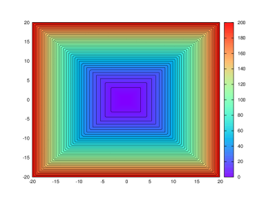
(a)

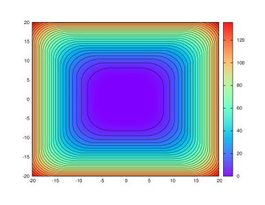
(b)

(c)

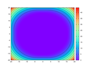
(d)

Figure 1. Evaluation of the solution $\phi((x_{1},x_{2},0,0,0,0,0,0)^{\dagger},t)$ of the HJ-PDE with initial data $J=\frac{1}{2}\|\cdot\|_{\infty}^{2}$ and Hamiltonian $H=\|\cdot\|_{2}$ for $(x_{1},x_{2})\,\in\,[-20,20]^{2}$ for different times $t$. Plots for $t=0,5,10,15$ and respectively depicted in (a), (b), (c) and (d). The level lines multiple of 5 are superimposed on the plots.

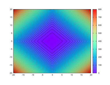
(a)

(b)

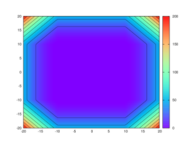
(c)

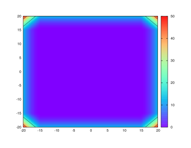
(d)

Figure 2. Evaluation of the solution $\phi((x_{1},x_{2},0,0,0,0,0,0)^{\dagger},t)$ of the HJ-PDE with initial data $J=\frac{1}{2}\|\cdot\|_{1}^{2}$ and Hamiltonian $H=\|\cdot\|_{1}$ for $(x_{1},x_{2})\,\in\,[-20,20]^{2}$ for different times $t$. Plots for $t=0,5,10,15$ are respectively depicted in (a), (b), (c) and (d). The level lines multiple of 20 are superimposed on the plots.

(a)

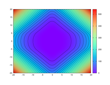
(b)

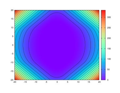
(c)

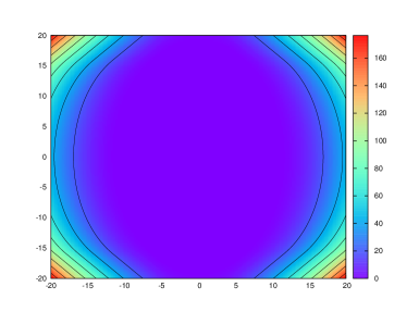
(d)

Figure 3. Evaluation of the solution $\phi((x_{1},x_{2},0,0,0,0,0,0)^{\dagger},t)$ of the HJ-PDE with initial data $J=\frac{1}{2}\|\cdot\|_{1}^{2}$ and Hamiltonian $H=\|\cdot\|_{D}$, for $(x_{1},x_{2})\,\in\,[-20,20]^{2}$ for different times $t$. Plots for $t=0,5,10,15$ are respectively depicted in (a), (b), (c) and (d). The level lines multiple of 20 are superimposed on the plots.

(a)

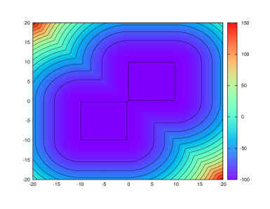
(b)

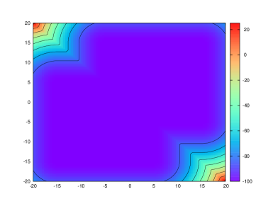
(c)

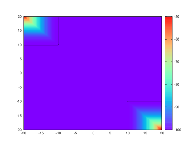
(d)

Figure 4. Evaluation of the solution $\phi((x_{1},x_{2},0,0,0,0,0,0)^{\dagger},t)$ of the HJ-PDE with initial data $J=\min{}\left(\frac{1}{2}\|\cdot\|_{2}^{2}-\langle b,\cdot\rangle,\frac{1}{2}\|\cdot\|_{2}^{2}+\langle b,\cdot\rangle\right)$ with $b=(1,1,1,1,1,1,1,1)^{\dagger}$ and Hamiltonian $H=\|\cdot\|_{1}$, for $(x_{1},x_{2})\,\in\,[-20,20]^{2}$ for different times $t$. Plots for $t=0,5,10,15$ are respectively depicted in (a), (b), (c) and (d). The level lines multiple of 15 are superimposed on the plots.

(a)

(b)

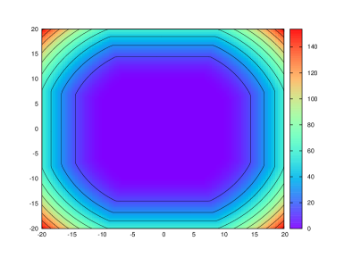
(c)

(d)

Figure 5. Evaluation of the solution $\phi((x_{1},x_{2},0,0,0,0,0,0)^{\dagger},t)$ of the HJ-PDE with initial data $J=\frac{1}{2}\|\cdot\|_{1}^{2}$ and Hamiltonian $H=\min{}\left(\|\cdot\|_{1},\sqrt{\langle\cdot,\frac{4}{3}D\cdot\rangle}\right)$, for $(x_{1},x_{2})\,\in\,[-20,20]^{2}$ for different times $t$. Plots for $t=2,5,9,12$ are respectively depicted in (a), (b), (c) and (d). The level lines multiple of 15 are superimposed on the plots.

5. Conclusion

We have designed algorithms which enable us to solve certain Hamilton-Jacobi equations very rapidly. Our algorithms not only evaluate the solution but also computes the gradient of the solution. These include equations arising in control theory leading to Hamiltonians which are convex and positively homogeneous of degree $1$. We were motivated by ideas coming from compressed sensing; we borrowed algorithms devised to solve $\ell_{1}$ regularized problems which are known to rapidly converge. We apparently extended this fast convergence to include convex positively 1-homogeneous regularized problems.

There are no grids involved. Instead of complexity which is exponential in the dimension of the problems, which is typical of grid based methods, ours appears to be polynomial in the dimension with very small constants. We can evaluate the solution on a laptop at about $10^{-4}-10^{-8}$ seconds per evaluation for fairly high dimensions. Our algorithm requires very low memory and is totally parallelizable which suggest that it is suitable for low energy embedded systems. We have chosen to restrict the presentation of the numerical experiments to norm-based Hamiltonians and we emphasize that our approach naturally extends to more elaborate positively 1-homogeneous Hamiltonians (using the min/max algebra results as we did for instance).

As an important step in this procedure we have also derived an equally fast method to find a closest point lying on $\Omega$, a finite union of compact convex sets $\Omega_{i}$, such that $\Omega=\cup_{i}^{k}\Omega_{i}$ has a nonempty interior, to a given point.

We can also solve certain so called fast marching [49] and fast sweeping [47] problems equally rapidly in high dimensions. If we wish to find $\psi:\mathbb{R}^{n}\to\mathbb{R}$ with, say $\psi=0$ on the boundary of a set $\Omega$ defined above, satisfying

$$\begin{cases}\|\nabla_{x}\psi(x)\|_{2}\;=\;1&\mbox{ in }\mathbb{R}^{n},\\ \psi(x)\;=\;0&\mbox{ for any }x\in(\Omega\setminus\mbox{int }\Omega),\end{cases}$$

then, we can solve for $u:\mathbb{R}^{n}\times[0,+\infty)\to\mathbb{R}$

$$\frac{\partial u}{\partial t}(x,t)\,+\,\|\nabla_{x}u(x)\|_{2}\;=\;0\quad\mbox{ in }\mathbb{R}^{n}\times(0,+\infty),$$

with initial data

$$\begin{cases}u(x,0)<0\mbox{ for any }x\in\mbox{int }\Omega,\\ u(x,0)>0\mbox{ for any }x\in(\mathbb{R}^{n}\setminus\Omega),\\ u(x,0)=0\mbox{ for any }x\in(\Omega\setminus\mbox{int }\Omega),\end{cases}$$

and locate the zero level set of $u(\cdot,t)=0$ for any given $t>0$. Indeed any $x\in\{y\in\mathbb{R}^{n}\;|\;u(y,t)\;=\;0\}$ satisfies $\psi(x)=t$.

Of course the same approach could be used for any convex, positively 1-homogeneous Hamiltonian $H$ (instead of $\|\cdot\|_{2}$), e.g., $H\,=\,\|\cdot\|_{1}$. This will give us results related to computing the Manhattan distance.

We expect to extend our work as follows:

1. We will do experiments involving linear controls, allowing $x$ and $t>0$ dependence while the Hamiltonian $(p,x,t)\mapsto H(p,x,t)$ is still convex and positively 1-homogeneous in $p$. The procedure was described in section 2.

2. We will extend our fast computation of the projection in several ways. We will consider in detail the case of polyhedral regions defined by the intersection of sets $\Omega_{i}\,=\,\{x\in\mathbb{R}^{n}\;|\;\langle a_{i},x\rangle-b_{i}\,\leq\,0\}$, $a_{i},b_{i}\,\in\,\mathbb{R}^{n}$, $\|a_{i}\|_{2}=1$, for $i=1,\dots,k$. This is of interest in linear programming (LP) and related problems. We expect to develop alternate approaches to several issues arising in LP, including rapidly finding the existence and location of a feasible point.

3. We will consider nonconvex but positively 1-homogeneous Hamiltonians. These arise in: differential games as well as in the problem of finding a closest point on the boundary of a given compact convex set $\Omega$, to an arbitrary point in the interior of $\Omega$.

4. As an example of a nonconvex Hamiltonians we consider the following problems arising in differential games [20]. We need to solve the following scalar problem for any $z\in\mathbb{R}^{n}$ and any $\alpha>0$

   $$\min_{y}\left\{\frac{1}{2}\|y-x\|_{2}^{2}-\alpha\|y\|_{1}\right\}.$$

   It is easy to see that the minimizer is the stretch₁ operator which we define for any $i=1,\dots,n$ as:

   (41) $$\left(\hbox{stretch}_{1}(x,\alpha)\right)_{i}\;=\;\begin{cases}x_{i}+\alpha&\hbox{if }\ x_{i}>0,\\ 0&\hbox{if }x_{i}=0,\\ x_{i}-\alpha&\hbox{if }\ x_{i}<0.\end{cases}$$

   We note that the discontinuity in the minimizer will lead to a jump in the derivatives $(x,t)\mapsto\frac{\partial\varphi}{\partial x_{i}}(x,t)$, which is no surprise, given that this interface associated with the equation

   $$\frac{\partial\varphi}{\partial t}(x,t)-\sum_{i=1}^{n}\left|\frac{\partial\varphi}{\partial x_{i}}(x,t)\right|\;=\;0,$$

   and the previous initial data, will move inwards, and characteristics will intersect. The solution $\varphi(x,t)$ will remain locally Lipschitz continuous, even though a point inside the ellipsoid may be equally close to two points on the boundary of the original ellipsoid in the Manhattan metric. So we are solving

   $$\varphi(x,t) =-\frac{1}{2}-\min_{v\in\mathbb{R}^{n}}\left\{\frac{1}{2}\sum_{i=1}^{n}a_{i}^{2}v_{i}^{2}-t\sum_{i=1}^{n}|v_{i}|+\langle x,v\rangle\right\}$$

   $$=-\frac{1}{2}+\frac{1}{2}\sum_{i=1}^{n}\frac{x_{i}^{2}}{a_{i}^{2}}-\min_{v\in\mathbb{R}^{n}}\left\{\frac{1}{2}\sum_{i}^{n}a_{i}^{2}\left(v_{i}-\frac{x_{i}}{a^{2}}\right)^{2}-t\sum_{i=1}^{n}|v_{i}|\right\}$$

   $$=-\frac{1}{2}+\frac{1}{2}\sum_{i=1}^{n}\frac{(|x_{i}|+t)^{2}}{a_{i}^{2}}$$

   The zero level set disappears when $t\geq\max_{i}a_{i}$ as it should.

   For completeness, we also consider the nonconvex optimization problem

   $$\min_{v\in\mathbb{R}^{n}}\left\{\frac{1}{2}\|v-x\|_{2}^{2}-\alpha\,\|v\|_{2}\right\}.$$

   Its minimizer is given by the $\mbox{stretch}_{2}$ operator formally defined by

   $$\mbox{stretch}_{2}(x,\alpha)\;=\;\begin{cases}x+\alpha\frac{x}{\|x\|_{2}}&\mbox{ if }x\neq 0,\\ \alpha\theta&\mbox{ with }\|\theta\|_{2}=1\mbox{ if }x=0.\end{cases}$$

   This formula, although multivalued at $x=0$, is useful to solve the following problem: move the unit sphere inwards with normal velocity $1$. The solution comes from finding the zero level set of

   $$\varphi(x,t) =-\min_{v\in\mathbb{R}^{n}}\left\{\frac{|v|_{2}^{2}}{2}-t\|v\|_{2}-\langle x,v\rangle\right\}-\frac{1}{2}$$

   $$=-\min_{v\in\mathbb{R}^{n}}\left\{\frac{1}{2}\|v-x\|_{2}^{2}-t\|v\|_{2}\right\}+\frac{1}{2}(\|x\|_{2}^{2}-1)$$

   $$=-\frac{1}{2}t^{2}+t\|x\|_{2}\left(1+\frac{t}{\|x\|_{2}}\right)+\frac{1}{2}(\|x\|_{2}^{2}-1)$$

   $$=\frac{1}{2}(\|x\|_{2}+t)^{2}-\frac{1}{2}$$

   and, of course, the zero level set is the set of $x$ satisfying $\|x\|_{2}=t-1$ if $t\leq 1$ and the zero level set vanishes for $t>1$.

Appendix A Gauge

Now suppose furthermore that we wish $H$ to be nonnegative, i.e., $H(p)\geq 0$ for any $p\in\mathbb{R}^{n}$. Under this additional assumption, we shall see that the Hamiltonian $H$ is not only the support function of $C$ but also the gauge of convex set that we will characterize. Let us define the gauge $\gamma_{\Omega}:\mathbb{R}^{n}\to\mathbb{R}^{n}\cup\{+\infty\}$ of a closed convex set $D$ containing the origin ([27, Def. 1.2.4, p. 202])

$$\gamma_{D}(x)\;=\;\inf\left\{\lambda>0\;|\>x\in\lambda D\right\},$$

where $\gamma_{D}(x)=+\infty$ if $x\notin\lambda D$ for all $\lambda>0$. Using [27, Thm. 1.2.5 (i), p 203], $\gamma_{D}$ is lower semicontinous, convex and positively 1-homogeneous. If $0\in\mbox{int }D$ then [27, Thm. 1.2.5 (ii), p. 203] the gauge $\gamma_{D}$ is finite everywhere, i.e., $\gamma_{D}:\mathbb{R}^{n}\to\mathbb{R}$, we recall that $\mbox{int }D$ denotes the interior of the set $D$. Thus, taking $H=\gamma_{D}$ satisfies our requirements. Note that if we further assume that $D$ is symmetric (i.e., for any $d\in D$ then $-d\in D$) then $\gamma_{D}$ is a seminorm. If in addition we wish $H(p)>0$ for any $p\in\mathbb{R}^{n}\setminus\{0\}$, then $D$ has to be a compact set ([27, Corollary. 1.2.6, p. 204]). For the latter case, a symmetric $D$ implies that $\gamma_{D}$ is actually a norm.

We now describe the connections between the sets $D$ and $C$, the gauge $\gamma_{D}$, the support function of $C$ and nonnegative, convex, positively 1-homogeneous Hamiltonians $H:\mathbb{R}^{n}\to\mathbb{R}$. Given a closed convex set $\Omega$ of $\mathbb{R}^{n}$ containing the origin, we denote by $\Omega^{\circ}$ the polar set of $\Omega$ defined by

$$\Omega^{\circ}\;=\;\left\{s\in\mathbb{R}^{n}\;|\;\langle s,x\rangle\leq 1\mbox{ for all }x\in\Omega\}\right\}.$$

We have that $(\Omega^{\circ})^{\circ}\,=\,\Omega$. Using [27, Prop. 3.2.4, p. 223] we have that the gauge $\gamma_{D}$ is the support function of $D^{\circ}$. In addition, [27, Corollary 3.2.5, p. 233] states that the support function of $C$ is the gauge of $C^{\circ}$. We can take $D\,=\,C^{\circ}$ and see that $H$ can be expressed as a gauge. Also, using [27, Thm. 1.2.5 (iii), p. 203] we have that $C^{\circ}\,=\,\{p\in\mathbb{R}^{n}\,|\,H(p)\leq 1\}$.

References

- [1] M. Akian, R. Bapat, and S. Gaubert. Max-plus algebras. In L. Hogben, editor, Handbook of Linear Algebra (Discrete Mathematics and Its Applications), volume 39. Chapman & Hall/CRC, 2006. Chapter 25.
- [2] J.-P. Aubin and A. Cellina. Differential Inclusions. Springer-Verlag, Berlin, 1984.
- [3] R. Bellman, Adaptive Control Processes, a Guided Tour, Princeton U. Press (1961).
- [4] R. Bellman, Dynamic Programming, Princeton U. Press, (1957).
- [5] H. Brezis. Opérateurs maximaux monotones et semi-groupes de contractions dans les espaces de Hilbert. North-Holland, 1973.
- [6] E.J. Candes, J. Romberg, and T. Tao, Exact Signal Reconstruction from Highly Incomplete Frequency Information, IEEE Trans. on Information Theory, v.52, (2), (2008), pp. 489-509.
- [7] A. Chambolle and J. Darbon. On total variation minimization and surface evolution using parametric maximum flows. International Journal of Computer Vision, 84(3):288–307, 2009.
- [8] A. Chambolle and T. Pock. A First-Order Primal-Dual Algorithm for Convex Problems with Applications to Imaging. Journal of Mathematical Imaging and Vision, 41(1):120-145, 2011.
- [9] L.T. Cheng and Y.H. Tsai. Redistancing by flow of time dependent eikonal equation. J. Comput. Phys. 227(8), 2008
- [10] P.L. Combettes and J.-C. Pesquet. Proximal thresholding algorithm for minimization over orthonormal bases. SIAM Journal on Optimization, 18(4):1351–1376, November 2007.
- [11] M.G. Crandall, L.C. Evans, and P.-L. Lions, Some Properties of Viscosity Solutions of Hamilton-Jacobi Equations, Trans. AMS, v.282, (2), (1984), pp. 487-502.
- [12] M.G. Crandall and P.-L. Lions, Viscosity Solutions of Hamilton-Jacobi Equations, Trans. AMS, v.277, (1), (1983), pp. 1-42.
- [13] J. Darbon. On Convex Finite-Dimensional Variational Methods in Imaging Sciences, and Hamilton-Jacobi Equations. SIAM Journal on Imaging Sciences 8:4, 2268-2293, 2015.
- [14] I. Daubechies, M. Defrise, and C. De Mol. An iterative thresholding algorithm for linear inverse problems with a sparsity constraint. Comm. Pure and Appl. Math., 57(11):1413–1457, 2004.
- [15] E.W. Dijkstra, A Note on Two Problems in Connexion ‘ with Graphs, Numer. Math., v.1, (1959), pp. 269-271.
- [16] I.C. Dolcetta, Representation of Solutions of Hamilton-Jacobi Equations, Nonlinear Equations: Methods, Models and Applications, (2003), pp. 79-90.
- [17] D.L. Donoho, Compressed Sensing, IEEE Trans. on Image Information Theory, v.52, (4), (2006), pp. 1289-1305.
- [18] I. Ekeland and R. Temam. Convex Analysis and Variational Problems. North-Holland, Amsterdam, 1976.
- [19] L.C. Evans, Partial Differential Equations, Grad. Studies in Mathematics, v. 19, AMS (2010).
- [20] L.C. Evans and P.E. Souganidis, Differential Games and Representation Formulas for Solutions of Hamilton-Jacobi Isaacs Equations, Indiana U. Math. J., v.38, (1984), pp. 773-797.
- [21] M.A.T. Figueiredo and R.D. Nowak. Bayesian wavelet-based signal estimation using non-informative priors. In Signals, Systems amp; Computers, 1998. Conference Record of the Thirty-Second Asilomar Conference on, volume 2, IEEE Piscataway, NJ 1998, pp. 1368–1373.
- [22] W. H. Fleming Deterministic nonlinear filtering. Annali della Scuola Normale Superiore di Pisa - Classe di Scienze, 25(3-4):435-454, 1997.
- [23] R. Glowinski and A. Marrocco, Sur l’approximation par éléments finis d’ordre, et la resolution par pénalzation-dualité, d’une classe de problemémes de Dirichlet non-linéares, C.R. hebd. Séanc. Acad. Sci., Paris 278, série A, (1974), pp. 1649-1652.
- [24] T. Goldstein and S. Osher, The Split Bregman Method for Regularized Problems, SIAM J. on Imaging Science, v.2, (2), 2009, pp. 323-343.
- [25] M.R. Hestenes, Multiplier and Gradient Methods, J. of Optimization Theory and Applications, v.4, (3), (1969), pp. 303-320.
- [26] J.-B. Hiriart-Urruty. Optimisation et Analyse Convexe. Presse Universitaire de France, 1998.
- [27] J.-B. Hiriart-Urruty and C. Lemaréchal. Convex Analysis and Minimization Algorithms Part I. Springer Verlag, Heidelberg, 1996.
- [28] J.-B. Hiriart-Urruty and C. Lemaréchal. Convex Analysis and Minimization Algorithms Part II. Springer Verlag, Heidelberg, 1996.
- [29] J. Eckstein and D.P. Bertsekas On the Douglas-Rachford splittingmethod and the proximal point algorithm for maximal monotone operators Math. Program., Ser. A 55(3), 2932̆013318 (1992).
- [30] E. Hopf, Generalized Solutions of Nonlinear Equations of the First Order, J. Math. Mech., v.14, (1965), pp. 951-973.
- [31] C. Hu and C.-W. Shu, A Discontinuous Galerkin Finite Element Method for Hamilton-Jacobi Equations, SIAM J. Sci. Comput., v.21, (2), (1999), pp. 666-690.
- [32] A. B. Kurzhanski and P. Varaiya Dynamics and Control of Trajectory Tubes: Theory and Computation. Birkhäuser, 2014 edition.
- [33] P.-L. Lions and B. Mercier. Splitting algorithms for the sum of two nonlinear operators. SIAM Journal on Numerical Analysis, 16(6):964–979, 1979.
- [34] P.-L. Lions and J-C Rochet. Hopf formula and multitime Hamilton-Jacobi equations. Proc. of American Mathmatical Socity, 96, no.1 (1986), 79–84.
- [35] W. M. McEneaney Max-Plus Methods for Nonlinear Control and Estimation . Birkhäuser, 2006 edition.
- [36] I.M. Mitchell, A.M. Bayen and C.J. Tomlin, A Time Dependent Hamilton-Jacobi Formulation of Reachable Sets for Continuous Dynamic Games, IEEE Trans on Automatic Control, v.50, 171, (2005), pp. 947-957.
- [37] I.M. Mitchell and C.J. Tomlin, Overapproximating Reachable Sets by Hamilton-Jacobi Projections, J. Sci. Comput., v.19, (1-3), (2003), pp. 323-346.
- [38] J.-J. Moreau. Proximité et dualité dans un espace hilbertien. Bulletin Spc. Math. France, 93, pp. 273–299, 1965.
- [39] A. Oberman and S. Osher and R. Takei and R. Tsai, Numerical methods for anisotropic mean curvature flow based on a discrete time variational formulation, Commun. Math. Sci., v.9, no. 3, pp.637-662, 2011.
- [40] S. Osher and B. Merriman, The Wulff Shape as the Asymptotic Limit of a Growing Crystalline Interface, Asian J. Mathematics, v.1, (3), (1997), pp. 560-571.
- [41] S. Osher and J.A. Sethian, Fronts Propagating with Curvature Dependent Speech: Algorithms Based on Hamilton-Jacobi Formulations, J. Comput. Phys., v.79, (1), (1988), pp. 12-49.
- [42] S. Osher and C.-W. Shu, High Order Essentially Nonosicllatory Schemes for Hamilton-Jacobi Equations, SIAM J. Numer. Analysis, v.28, (4), (1991), pp. 907-922.
- [43] S. Osher and W. Yin, Error Forgetting of Bregman Iteration, J. Sci. Comput., v.54, (2), (2013), pp. 684-695.
- [44] R.T. Rockafellar. Convex Analysis. Princeton Landmarks in Mathematics. Princeton University Press, Princeton (1997). Reprint of the 1970 original, Princeton Paperbacks.
- [45] R.T. Rockafellar Monotone operators and the proximal point algorithm. SIAM J. Control Optim. 14(5), 877-898 (1976).
- [46] R.T. Rockafellar. Network Flows and Monotropic Optimization. Reprint of the 1984 original. Athena Scientific, 1998.
- [47] Y.-H. R. Tsai, L.-T. Cheng, S. Osher, and H.-K. Zhao. Fast Sweeping Algorithms for a Class of Hamilton–Jacobi Equations SIAM Journal on Numerical Analysis 41:2, 673-694, 2003.
- [48] M. Teboulle Convergence of Proximal-like Algorithms. SIAM J. Optimization 7 (1997), 1069-1083.
- [49] J. N. Tsitsiklis Efficient algorithms for globally optimal trajectories. Automatic Control, IEEE Transactions on , vol.40, no.9, pp.1528-1538, Sep 1995
- [50] G. Winkler. Image Analysis, Random Fields and Dynamic Monte Carlo Methods. Applications of mathematics. 2nd edition, Springer-Verlag, 2006.
- [51] W. Yin, S. Osher, D. Goldfarb, and J. Darbon, Bregman Iterative Algorithms for Minimization with Applications to Compressed Sensing, SIAM J. on Imaging Sci., v.1 (1), (2008), pp. 143-168.
- [52] Y.T. Zhang and C.-W. Shu, High Order WENO Schemes for Hamilton-Jacobi Equations on Triangular Meshes, SIAM J. on Sci. Comput., v.24, (3), (2013), pp. 1005-1030.
- [53] M. Zhu and T.F. Chan, An Efficient Primal-Dual Hybrid Gradient Algorithm For Total Variation Image Restoration, UCLA CAM Report 08-34, 2008.