Superconductivity at very low density: the case of strontium titanate
Abstract
Doped strontium titanate becomes superconducting at a density as low as , where the Fermi energy is orders of magnitude smaller than the longitudinal-optical-phonon frequencies. In this limit the only optical mode with a frequency which is smaller than the Fermi energy is the plasmon. In contrast to metals, the interaction strength is weak due to screening by the crystal, which allows the construction of a controllable theory of plasmon superconductivity. We show that plasma mediated pairing alone can account for the observed transition temperatures if the screening by the crystal is reduced in the slightly doped samples compared with the insulating ones. This mechanism can also explain the pairing in the two-dimensional superconducting states observed at surfaces and interfaces with other oxides. We also discuss unique features of the plasmon mechanism, which appear in the tunneling density of states above the gap.
Introduction – The BCS theory very successfully explains superconductivity in metals. The essential attraction between electrons, according to this theory, is generated by exchange of phonons, which have a characteristic frequency . A crucial condition for the applicability of the theory is the ’retardation’ condition, namely that , where is the Fermi energy Bogoliubov et al. (1960). This condition holds in almost all known conventional superconductors and seems to be a universal property.
An outstanding exception is doped strontium titanate (SrTiO3). Free charge carriers in this material are achieved by inducing oxygen vacancies or doping with elements such as La or Nb. Superconductivity is typically observed at temperatures lower than a few hundreds of Milikelvins Schooley et al. (1964). The transition temperature exhibits a dome shape as a function of carrier concentration, which extends to surprisingly low densities Koonce et al. (1967); Binnig et al. (1980); Baratoff and Binnig (1981); Lin et al. (2014). Recently it has been reported that superconductivity extends to densities as low as where the Fermi energy is 1meV Lin et al. (2013). In this situation is certainly not greater than , and therefore BCS theory does not apply. The natural question is therefore, why is strontium titanate superconducting at such a low density?
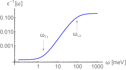
SrTiO3 also exhibits non-trivial phenomena in its insulating state. Upon cooling, the polarizability of this material diverges with a Cuire-Weiss behavior signaling a ferroelectric instability. However, this behavior is cutoff before the instability is reached and eventually strontium titanate remains paraelectric all the way down to zero temperature Weaver (1959); Müller and Burkard (1979). The soft transverse optical phonon associated with the instability leads to a huge dielectric constant which, for our purposes, can be approximated by a single resonance model
| (1) |
where meV is the frequency of the transverse mode at Vogt (1995); Vogt and Rossbroich (1981), Kamarás et al. (1995) and Weaver (1959). The Coulomb interaction has a pole at the frequency of the longitudinal phonon mode, , which is related to the transverse one by the Lyddane-Sachs-Teller (LST) relation .
Gurevich, Larkin and Firsov (GLF) Gurevich et al. (1962) were the first to point out the potential importance of the longitudinal phonon mode to superconductivity. They considered the attractive electron-electron interaction mediated by long-range Coulomb potentials induced this mode. Therefore, in their theory the frequency plays the role of in the BCS theory. For the parameters used in Eq. 1 one obtains , such that . It is therefore not possible to use the longitudinal mode to explain the superconducting state of SrTiO3.
Early theoretical studies of superconductivity in SrTiO3 Koonce et al. (1967) assumed multiple valleys and emphasized the importance of intervalley phonon scattering. These assumptions are now known to be incorrect. Later, Takada Takada (1980), added dynamical electronic screening to the GLF model Gurevich et al. (1962) and used the theory of Ref. Kirzhnits et al. (1973) to calculate , again with very good agreement with experiment. Interestingly, Takada proposed that plasma oscillations participate in mediating the attractive interactions. However, his theory is uncontrolled because he incorporates the longitudinal phonon and the plasmon as mediators of a attractive interaction even when their frequencies are significantly larger than the Fermi energy, which is known to be problematic Grabowski and Sham (1984); Grimaldi et al. (1995). Indeed, his attraction is mainly generated by the higher frequency mode, i.e. the phonon at low density and the plasmon at higher density (see for example the conclusions in Ref.Klimin et al. (2014)).
We would also like to note two recent studies of phonon-mediated superconductivity in SrTiO3. Ref. Gor‘kov (2016) argued that multiplicity of longitudinal optical phonons leads to instantaneous attraction between electrons. In the SI we show that this is not possible in the standard picture of screening due to polar phonons. Ref. Edge et al. (2015) tied the dome shape of to softening of the ferroelectric mode observed in DFT calculations. But the coupling to the transverse mode is too weak when the density of states is so small.
In this paper we revisit the question of superconductivity in SrTiO3 in light of new data using the Eliashberg theory. Our approach is to construct a controllable theory and focus on the extreme low density limit where the open questions are clearest. In this limit the screened plasma frequency is the only resonance of the interaction that occurs below the Fermi energy, and therefore we agree with Ref. Takada (1980) that it is an important mechanism for pairing of electrons. Our theory is controlled by weak coupling to the plasmon, which is provided by the screening of the crystal. However, unlike Ref. Takada (1980), we find that the coupling is too weak if the dielectric constant measured in insulating SrTiO3 Weaver (1959); Vogt and Rossbroich (1981); Kamarás et al. (1995) is used. Given our belief that the plasmon is the only low lying mode that is capable of inducing pairing, we find that the only way to obtain a realistic transition temperature at the lowest measured density is to reduce the dielectric screening to . This reduction may result from local hardening of the soft mode induced by the doping sites Bäuerle et al. (1980); Crandles et al. (1999); van Mechelen et al. (2008).
We also find that upon rasing the density the Lifshitz transitions observed by Ref. Lin et al. (2014) have a weak effect on . The interaction between the plasmon and the longitudinal optical phonon has a much stronger effect and leads to a suppression of at high density (see Fig. 1). We also show that the plasmon mechanism for superconductivity can explain the observed transition temperatures in two-dimensional gases based on SrTiO3 Caviglia et al. (2008); Ueno et al. (2008). Finally, we show that the plasmon leads to a density dependant feature in the tunneling density of states (see Fig. 4).
Model – For simplicity the three conduction bands near the -point are taken to be isotropic and parabolic with a dispersion , where labels the bands. We take , Lin et al. (2014) and , and with and . We start our analysis from the lowest density, where and only the lowest band is occupied. Therefore all quantities refer to the lowest band unless explicitly specified otherwise.
To describe the interactions between the electrons we consider only long-range Coulomb forces, and use the random-phase-approximation
| (2) |
where is the electronic polarization and is given by Eq. 1.
plasma osculations in a slightly doped ionic crystal – Before estimating the transition temperature from Eq. 2 we discuss the interaction between the electronic and ionic longitudinal modes. At long wavelengths the electronic polarization leads to a plasma mode , which hybridizes with the longitudinal mode (see SI and Refs. Mooradian and Wright (1966); Cohen (1969)). When the plasma frequency is reduced to due to screening by the crystal. On the other hand if the plasma mode takes its bare value and screens the electric fields induced by the longitudinal mode . As a result the gap between and at disappears and the phonon mode decouples from the electrons Mahan (2013).
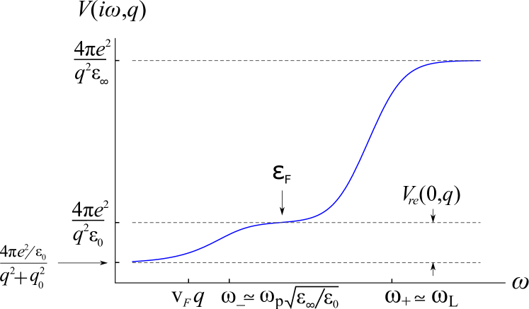
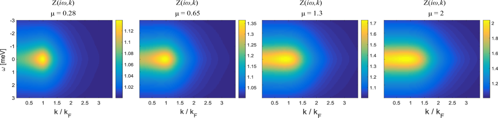
Both of these limits are realized in doped strontium titanate. In what follows we focus low density, i.e. cm-3 where the plasma frequency is lower than and therefore there is a small plasma mode lying below the Fermi energy. Fig. 2 presents the interaction Eq. 2 in this limit. As can be seen the interaction is essentially frequency independent in the vicinity of and it is physically obvious that the frequency dependence at the scale of cannot give rise to pairing. Nevertheless, all earlier studies Koonce et al. (1967); Appel (1969); Eagles (1969); Takada (1980); Klimin et al. (2014) assume that Eliashberg theory continues to hold and integrate the interaction up to many times ( in the case of Ref. Takada (1980)) to obtain . The problem is that electronic states far above the Fermi level are involved, and there is no reason to single out the Eliashberg paring diagrams as the dominant ones. This problem has been emphasized by Ref. Grabowski and Sham (1984) which showed that inclusion of vertex corrections rapidly kill once the frequency of the bosons that are being exchanged become comparable to . This work explains why previous proposals Takada (1978); Rietschel and Sham (1983) of the plasmon exchange mechanism in metals are not valid, because otherwise very high transition temperatures are predicted. Form this point of view the novelty of SrTiO3 is that due to crystal screening the plasmon is weakly coupled and can be smaller than .
Our departure from previous work is to insist that when the energy scale is much lower than , we live in a world where the bare Coulomb repulsion is replaced by , which sets the strength of the interaction. We therefore restrict our frequency integration to and below when we solve the Eliashberg equation. For this leads to the interaction
| (3) |
where is the screened Thomas-Fermi wavelength and is the density of states of the lowest conduction band. To relate to standard Eliashberg theory we decompose the interaction into two parts: a static repulsive part and the retarded attractive piece .
Considering the interaction in Eq. 3 as a source for superconductivity we immediately encounter a problem. If we assume that slightly doped SrTiO3 has the same as undoped SrTiO3, the effective coupling strength is of order and there is no hope of getting any measurable . This forces us to use as a phenomenological parameter (and therefore , if we continue to assume the validity of the LST relation) and see what we need to set a measurable . We do this by considering dependance of the transverse frequency on doping
| (4) |
where Vogt (1995); van Mechelen et al. (2008). and control the onset density and the high density saturation frequency, respectively. The reduction of is obtained from Eq. 4 through the LST relation . As we see below, at the lowest density we need . At the end of the paper we speculate how local stiffening of Bäuerle et al. (1980); Crandles et al. (1999); van Mechelen et al. (2008) can lead to suppression of in the vicinity of the doping sites.
Eliashberg theory – To solve for the superconducting gap we employ the Eliashberg theory Eliashberg (1960). For brevity we do not derive the self-consistent equations (for a review see Ref. Margine and Giustino (2013)). We consider all three self-consistent equations for the the case in which the gap has -wave symmetry, which are given by
| (5) | |||
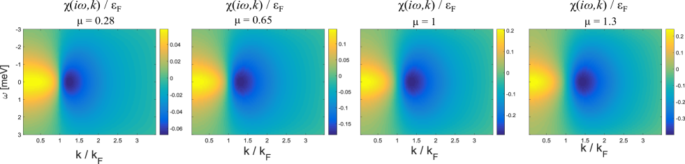
where and . Here , and represent the mass renormalization, the dispersion renormalization and the superconducting order-parameter appearing in the self-energy corrections to the Green’s function
| (6) |
where and the Pauli matrices act in Nambu space .
The brackets in Eq. (5) denote averaging over the solid angle such that . The angular integration over the retarded part of the interaction is cutoff at large angles when where the interaction in Eq. 2 becomes statically screened (see Fig.2). As a result the height of the Lorentzian in Eq. 3 is reduced compared to the static part by
which is nothing but the solid angle average of Eq. 2 in the limit of .
To solve the Eliashberg equations Eq. 5 numerically we truncate the sum over Matsubara frequencies by setting a cutoff frequency . In conventional Eliashberg theory the renormalization of the static Coulomb interaction due to integration over frequencies higher than the cutoff is taken into account by the phenomenological Coulomb pseudo-potential . Here we will need to introduce a similar phenomenological parameter, which is a dimensionless ratio
| (7) |
Note that the conventional is related to through the double momentum average on the Fermi surface Margine and Giustino (2013). The solution of Eq. 5 is then obtained by iteration of the equations starting from the initial state , and if and zero otherwise.
The momentum dependence of the solutions of Eq. 5 strongly depends on the coupling strength (see SI). For strong coupling the order parameter extends far away from the Fermi surface. However, at weak coupling it becomes sharply peaked, signaling that most of the pairing occurs in a narrow window around . Therefore, we further simplify Eq. 5 by restricting the momentum integration to the vicinity of the Fermi surface by integrating the strong momentum dependence coming from the dispersion in and from the Coulomb interaction while setting to in all other quantities. In this limit the dispersion renormalization also becomes much smaller than and can be neglected (see SI). We emphasize that this procedure is valid only at weak coupling.
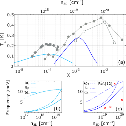
The calculated transition temperature is plotted in Fig. 1.a for two different sets of parameters. The blue curve corresponds to , , and , and cyan to , , and . Here the higher density dome is taken with a higher mass due to the mass enhancement measured by Ref. Lin et al. (2014). We also plot the plasma frequency , the Fermi energy and the frequency of the transverse mode for each one of these sets in Fig. 1.b and Fig. 1.c. The transition temperature is compared with the experimental data points (grey) taken from Refs.Schooley et al. (1964); Lin et al. (2014).
The reduction of at higher doping occurs because the plasma frequency grows and becomes comparable to , where the two modes hybridize. In this limit the electron gas begins to screen to the crystal fields and not vice versa, which leads to a decoupling of the longitudinal optical mode from the electrons (see SI). Therefore, the plasmon mechanism cannot explain superconductivity in the high density regime .
Superconductivity in two-dimensions –
A variety of two-dimensional electron gases have been realized in SrTiO3 (for example Refs. Ohtomo and Hwang (2004); Santander-Syro et al. (2011)). These gases become superconducting with a transition temperature which is similar to the bulk Ueno et al. (2008); Caviglia et al. (2008). Therefore, it is interesting to understand whether the plasmon mechanism described here is relevant in two-dimensions. We note that in this case the observed superconductivity is limited to rather high doping levels (see Fig. 1.a), where ,
To address this question we repeat the derivation of the Eliashberg equations for case of two-dimensions (see SI). A crucial difference is that now the plasma frequency is not gapped . This leads to a small attractive interaction below the Fermi energy even when the doping level is high. Additionally, the reduction of (or the stiffining of ) are much more natural due to the electric fields near the surface. Since there are no systematic measurements, we simply assume a constant , which corresponds to .
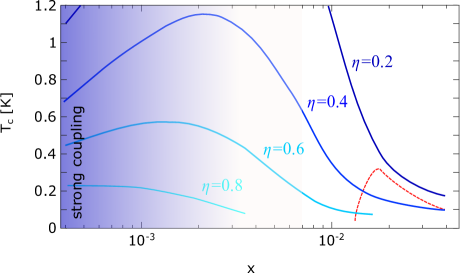
The calculated transition temperature vs. density for a single band model with is plotted in Fig. 3 for different values of . Note that here we have taken also smaller values of because the Fermi energy is larger and the traditional renormalization applies (see SI). The shaded region is where the coupling strength becomes large and the Eliashberg theory should not be trusted. The red dashed line is a typical dome from experiments Caviglia et al. (2008); Richter et al. (2013).
As can be seen at lower density the calculated dome does not agree with experiment, and extends to very low density where the localization is observed Caviglia et al. (2008). This discrepancy is actually consistent with the findings of Ref. Richter et al. (2013), which report pseudogap behavior in this regime. Therefore, the reduction of at lower density results from phase fluctuations and not decreasing of the pairing gap, such that the mean-field is much higher than the observed one.
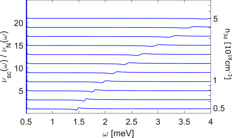
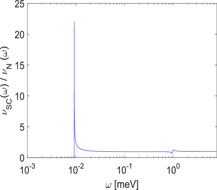
Tunneling density of states – We now turn to discuss a feature of plasmonic superconductivity which show in the single particle tunneling density of states (TDOS) above the gap. The TDOS of a standard BCS superconductor displays fingerprints of phonon resonances Schrieffer et al. (1963). As we show here, and for the same reason, the plasma frequency in dilute SrTiO3 should also become observable.
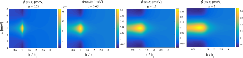
We obtain the TDOS from the imaginary part of the analytically continued Green’s function (Eq. 6), which is calculated using a controlled Padé approximation (for details see Ref. Beach et al. (2000) and SI). In Fig. 4 we plot the TDOS for different values of ranging between and at a temperature and using , , and . The spectral line-shape of the plasmon exhibits strong density dependence which is not expected in the case of phonon mediated superconductivity.
Discussion – We claim that the plasmon is the only bosonic mode capable of explaining superconductivity in dilute SrTIO3. On the other hand we need to assume reduction of crystal screening by considering the stiffening of the soft ferroelectric mode induced by defects. The defects may result from oxygen vacancies Bäuerle et al. (1980); Crandles et al. (1999) or from chemical dopants (Nb, La, etc.) van Mechelen et al. (2008). These defects induce pinning potentials and long range distortions, and it is known that is highly sensitive to strain induced by pressure or stress due to the proximity of the ferroelectric transition Venturini et al. (2003); Worlock and Fleury (1967). The oxygen vacancies are expected to have a stronger effect than substitutional disorder. We account for this difference by using different onset densities for the stiffening which leads to the two domes in Fig. 1. In this scenario the two domes observed by Ref. Lin et al. (2014) are related to different doping techniques and possibly differences in the sample properties (for example in Ref. de Lima et al. (2015) the relatively low value of measured in their pristine SrTiO3) rather than the Lifshitz transitions. It is also important to emphasize that the values of presented in Fig. 1 have been inferred from the LST relation, which may breakdown due to disorder.
The plasmon mechanism cannot explain superconductivity at higher density regime, , (see Fig. 1) because the plasma frequency becomes larger than . Interestingly, Ref. Meevasana et al. (2010) estimated the electron-phonon coupling strength to the lowest longitudinal mode , and found it to be moderate. It is therefore possible that this mode is mainly responsible for the pairing at higher densities.
An interesting aspect of the plasmonic mechanism in two-dimensions is that it is expected to be highly sensitive to external metallic gates. If a high density metal is deposited close enough to the two-dimensional superconductor the long-ranged Coulomb potentials will be screened, which should dramatically modify the dispersion of the plasma mode. Therefore, it is interesting to understand the effects of external metallic gates on the superconducting states in two-dimensions.
Finally, It is compelling to understand whether the plasmonic mechanism is relevant to other materials? According to our predictions the important ingredients are a dilute electron gas with relatively large effective mass and strong dielectric screening such that the plasma frequency lies below the Fermi level. The recently discovered superconductors in doped topological insulators Hor et al. (2010); Wray et al. (2010); Kriener et al. (2011); Liu et al. (2015) are candidates which may match these criterions, where the large dielectric screening is naturally present due to the small band gap.
Acknowledgments – We are grateful to Leonid Levitov for insightful discussions which helped launch this project and to Nandini Trivedi and Mohit Randeria for helpful discussions. JR acknowledges the Gordon and Betty Moore Foundation under the EPiQS initiative under grant no. GBMF4303. PAL acknowledges the support of DOE under grant no. FG02-03ER46076.
References
- Bogoliubov et al. (1960) N. N. Bogoliubov, V. Tolmachev, and D. Shirkov, Consultants Bureau, New York (1960).
- Schooley et al. (1964) J. Schooley, W. Hosler, and M. L. Cohen, Physical Review Letters 12, 474 (1964).
- Koonce et al. (1967) C. Koonce, M. L. Cohen, J. Schooley, W. Hosler, and E. Pfeiffer, Physical Review 163, 380 (1967).
- Binnig et al. (1980) G. Binnig, A. Baratoff, H. E. Hoenig, and J. G. Bednorz, Phys. Rev. Lett. 45, 1352 (1980).
- Baratoff and Binnig (1981) A. Baratoff and G. Binnig, Physica B+ C 108, 1335 (1981).
- Lin et al. (2014) X. Lin, G. Bridoux, A. Gourgout, G. Seyfarth, S. Krämer, M. Nardone, B. Fauqué, and K. Behnia, Physical Review Letters 112, 207002 (2014).
- Lin et al. (2013) X. Lin, Z. Zhu, B. Fauqué, and K. Behnia, Physical Review X 3, 021002 (2013).
- Weaver (1959) H. Weaver, Journal of Physics and Chemistry of Solids 11, 274 (1959).
- Müller and Burkard (1979) K. A. Müller and H. Burkard, Phys. Rev. B 19, 3593 (1979).
- Vogt (1995) H. Vogt, Phys. Rev. B 51, 8046 (1995).
- Vogt and Rossbroich (1981) H. Vogt and G. Rossbroich, Phys. Rev. B 24, 3086 (1981).
- Kamarás et al. (1995) K. Kamarás, K.-L. Barth, F. Keilmann, R. Henn, M. Reedyk, C. Thomsen, M. Cardona, J. Kircher, P. L. Richards, and J.-L. Stehlé, Journal of Applied Physics 78, 1235 (1995).
- van Mechelen et al. (2008) J. L. M. van Mechelen, D. van der Marel, C. Grimaldi, A. B. Kuzmenko, N. P. Armitage, N. Reyren, H. Hagemann, and I. I. Mazin, Phys. Rev. Lett. 100, 226403 (2008).
- Gurevich et al. (1962) L. V. Gurevich, A. I. Larkin, and Y. A. Firsov, Sov. Phys. Sol. State 4, 131 (1962).
- Takada (1980) Y. Takada, Journal of the Physical Society of Japan 49, 1267 (1980).
- Kirzhnits et al. (1973) D. Kirzhnits, E. Maksimov, and D. Khomskii, Journal of Low Temperature Physics 10, 79 (1973).
- Grabowski and Sham (1984) M. Grabowski and L. J. Sham, Physical Review B 29, 6132 (1984).
- Grimaldi et al. (1995) C. Grimaldi, L. Pietronero, and S. Strässler, Phys. Rev. Lett. 75, 1158 (1995).
- Klimin et al. (2014) S. N. Klimin, J. Tempere, J. T. Devreese, and D. van der Marel, Phys. Rev. B 89, 184514 (2014).
- Gor‘kov (2016) L. P. Gor‘kov, Proc. Natl. Acad. Sci. 113, 4646 (2016).
- Edge et al. (2015) J. M. Edge, Y. Kedem, U. Aschauer, N. A. Spaldin, and A. V. Balatsky, Phys. Rev. Lett. 115, 247002 (2015).
- Bäuerle et al. (1980) D. Bäuerle, D. Wagner, M. Wöhlecke, B. Dorner, and H. Kraxenberger, Zeitschrift für Physik B Condensed Matter 38, 335 (1980).
- Crandles et al. (1999) D. A. Crandles, B. Nicholas, C. Dreher, C. C. Homes, A. W. McConnell, B. P. Clayman, W. H. Gong, and J. E. Greedan, Phys. Rev. B 59, 12842 (1999).
- Caviglia et al. (2008) A. Caviglia, S. Gariglio, N. Reyren, D. Jaccard, T. Schneider, M. Gabay, S. Thiel, G. Hammerl, J. Mannhart, and J.-M. Triscone, Nature 456, 624 (2008).
- Ueno et al. (2008) K. Ueno, S. Nakamura, H. Shimotani, A. Ohtomo, N. Kimura, T. Nojima, H. Aoki, Y. Iwasa, and M. Kawasaki, Nature materials 7, 855 (2008).
- Mooradian and Wright (1966) A. Mooradian and G. B. Wright, Phys. Rev. Lett. 16, 999 (1966).
- Cohen (1969) M. L. Cohen, SUPERCONDUCTIVITY IN LOW-CARRIER-DENSITY SYSTEMS: DEGENERATE SEMICONDUCTORS., edited by R. D. Parks (New York, Marcel Dekker, Inc., 1969).
- Mahan (2013) G. D. Mahan, Many-particle physics (Springer Science & Business Media, 2013).
- Appel (1969) J. Appel, Phys. Rev. 180, 508 (1969).
- Eagles (1969) D. M. Eagles, Phys. Rev. 186, 456 (1969).
- Takada (1978) Y. Takada, Journal of the Physical Society of Japan 45, 786 (1978).
- Rietschel and Sham (1983) H. Rietschel and L. J. Sham, Phys. Rev. B 28, 5100 (1983).
- Eliashberg (1960) G. M. Eliashberg, Sov. Phys. Sol. JETP 11, 696 (1960).
- Margine and Giustino (2013) E. R. Margine and F. Giustino, Phys. Rev. B 87, 024505 (2013).
- Meevasana et al. (2010) W. Meevasana, X. J. Zhou, B. Moritz, C.-C. Chen, R. H. He, S.-I. Fujimori, D. H. Lu, S.-K. Mo, R. G. Moore, F. Baumberger, T. P. Devereaux, D. van der Marel, N. Nagaosa, J. Zaanen, and Z.-X. Shen, New Journal of Physics 12, 023004 (2010).
- Richter et al. (2013) C. Richter, H. Boschker, W. Dietsche, E. Fillis-Tsirakis, R. Jany, F. Loder, L. Kourkoutis, D. Muller, J. Kirtley, C. Schneider, et al., Nature 502, 528 (2013).
- Ohtomo and Hwang (2004) A. Ohtomo and H. Hwang, Nature 427, 423 (2004).
- Santander-Syro et al. (2011) A. Santander-Syro, O. Copie, T. Kondo, F. Fortuna, S. Pailhes, R. Weht, X. Qiu, F. Bertran, A. Nicolaou, A. Taleb-Ibrahimi, et al., Nature 469, 189 (2011).
- Worlock and Fleury (1967) J. Worlock and P. Fleury, Physical Review Letters 19, 1176 (1967).
- Sirenko et al. (2000) A. Sirenko, C. Bernhard, A. Golnik, A. M. Clark, J. Hao, W. Si, and X. Xi, Nature 404, 373 (2000).
- Bell et al. (2009) C. Bell, S. Harashima, Y. Kozuka, M. Kim, B. G. Kim, Y. Hikita, and H. Y. Hwang, Phys. Rev. Lett. 103, 226802 (2009).
- Schrieffer et al. (1963) J. R. Schrieffer, D. J. Scalapino, and J. W. Wilkins, Phys. Rev. Lett. 10, 336 (1963).
- Beach et al. (2000) K. Beach, R. Gooding, and F. Marsiglio, Physical Review B 61, 5147 (2000), arXiv:9908477 [cond-mat] .
- Venturini et al. (2003) E. L. Venturini, G. A. Samara, and W. Kleemann, Phys. Rev. B 67, 214102 (2003).
- de Lima et al. (2015) B. de Lima, M. da Luz, F. Oliveira, L. Alves, C. dos Santos, F. Jomard, Y. Sidis, P. Bourges, S. Harms, C. Grams, et al., Physical Review B 91, 045108 (2015).
- Eagles (1965) D. Eagles, Journal of Physics and Chemistry of Solids 26, 672 (1965).
- Hor et al. (2010) Y. S. Hor, A. J. Williams, J. G. Checkelsky, P. Roushan, J. Seo, Q. Xu, H. W. Zandbergen, A. Yazdani, N. P. Ong, and R. J. Cava, Phys. Rev. Lett. 104, 057001 (2010).
- Wray et al. (2010) L. A. Wray, S.-Y. Xu, Y. Xia, Y. San Hor, D. Qian, A. V. Fedorov, H. Lin, A. Bansil, R. J. Cava, and M. Z. Hasan, Nature Physics 6, 855 (2010).
- Kriener et al. (2011) M. Kriener, K. Segawa, Z. Ren, S. Sasaki, and Y. Ando, Physical review letters 106, 127004 (2011).
- Liu et al. (2015) Z. Liu, X. Yao, J. Shao, M. Zuo, L. Pi, S. Tan, C. Zhang, and Y. Zhang, arXiv preprint arXiv:1502.01105 (2015).
- Zhong et al. (1994) W. Zhong, R. D. King-Smith, and D. Vanderbilt, Phys. Rev. Lett. 72, 3618 (1994).
- Kozii and Fu (2015) V. Kozii and L. Fu, Phys. Rev. Lett. 115, 207002 (2015).
Superconductivity at very low density: the case of strontium titanate - Supplementary Information
I Optical phonon spectrum in
In this section we review the dielectric properties of insulating strontium titanate including three active optical modes and discuss the applicability of the single resonance model. We also explain our disagreement with the screened interaction used in a recent preprint (Ref. Gor‘kov (2016)).
The dielectric function comes from the sum of the polarizability of various transverse modes
| (8) |
In the experimental literature the crystal dielectric constant is traditionally presented as a product
| (9) |
which makes it explicit that and are the zeros and poles of the dielectric constant, respectively. The limit leads to the Lyddane-Sachs-Teller relation.
The experimentally measured values of the longitudinal and transverse frequencies in insulating SrTiO3 are given by Vogt and Rossbroich (1981); Kamarás et al. (1995) and .
It is convenient to decompose the inverse dielectric constant (or equivalently the screened Coulomb interaction) into a sum of resonances
| (10) |
Eq. 10 has the interpretation that the screened interaction is given by the bare Coulomb repulsion reduced by the contributions from each modes. Using the experimentally measured values for the parameters in Eq. 9 one gets , and Eagles (1965). Thus we find that that the coupling to the lowest mode and is weak. This is also seen from Eq. 9 by noting that and so that their contribution to Eq. 9 cancel each other, leaving only . This is consistent with the conclusions of Ref. Zhong et al. (1994) which find that the lowest transverse mode is most closely related to the largest longitudinal mode . Therefore we can use the single resonance model
| (11) |
where . We therefore neglect the index j in the main text and identify and . The full dielectric constant, including the contributions from 3 modes, is plotted in Fig. 5 which indeed resembles a wide single resonance with transverse frequency and longitudinal frequency .
It is however interesting to point out that Ref. Meevasana et al. (2010) estimated a moderate coupling to the first longitudinal mode, which is much stronger than the values given earlier after Eq. 10 Eagles (1965). This estimate is based on the self-energy correction to the electron dispersion measured by photoemission and involves involves a finite value of , whereas the optical measurement of are for thus it is possible that coupling is stronger at finite and it could be that the mode at plays an important role and that at higher density, where the chemical potential is higher than it also participates in the pairing. In any case we are mostly interested in the case where the Fermi energy is significantly lower than .
We remark that from Eq. 8 and Eq. 9 it is clear that is always positive, i.e. the Coulomb interaction screened by polar phonons is always positive when the frequencies are expressed in Matsubara space. In particular, the static interaction is always repulsive. This feature however is not explicit in Eq. 10. Nevertheless, there must be constraints on the parameters so that Eq. 10 also satisfies the positivity requirement, i.e. cannot be chosen as free parameters.
A recent paper by Gor’kov Gor‘kov (2016) appears to have fallen prey to this pitfall. He argues that in SrTiO3 the mode is mainly responsible for the large and he introduces (as we do) the standard form of the interaction in the case of a single phonon resonance (his Eq. 1)
| (12) |
As mentioned the last term on the R.H.S. of Eq. 12 may be interpreted as the phonon mediated interaction and corresponds to our Eq. 10 with a single mode. Gor’kov then argues that since the static repulsion is very small it can be overcome by contributions from and if he added their contributions to Eq. 12 as in Eq. 10. The problem with this argument is that from Eq. 10 and Eq. 9, and also contributed to and adding their contributions again will be double counting. Furthermore, as we discussed earlier, their coupling strengths and are not arbitrary, but subject to the constraint is always positive. For this reason we disagree with his conclusion that a static attractive interaction can be achieved by polar phonon screening.
II interaction between optical phonons and free charge carriers
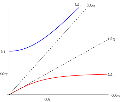
In the main text we have briefly discussed the interplay between the plasma oscillations and the low- behavior of the optical modes in a polar crystal. We have also discussed the behavior at two limiting cases, namely in the limit , where the longitudinal oscillations are much faster than the plasma and therefore simply screen the interaction and modify to . On the other hand in the opposite limit, where , the plasma is fast enough to completely screen the long range forces induced by the longitudinal mode and therefore the coulomb deriven gap between the longitudinal and transverse modes disappears. In this section we will make this discussion formal and describe the behavior over the whole range including the hybridization region.
For this purpose we consider the interaction (Eq. 2 in the main text) in the limit where . In this case the polarization bubble can be approximated by and the interaction assumes the formCohen (1969); Mahan (2013)
| (13) |
where is the bare plasma frequency, is the bare Thomas-Fermi momentum,
| (14) |
| (15) |
and .
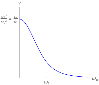
The poles of the interaction and the coupling constant are plotted in Figs. 6 and 7 as a function of the bare plasma frequency . We identify two distinct regimes: (a) For , we have , and . Therefore, in this limit the lower frequency pole corresponds to a plasmon in an interaction which is fully screened by the dielectric. (b) In the opposite limit, we have , and . Therefore the plasma frequency takes it’s bare value and completely shields the optical phonon.
Doped strontium titanate goes through both of these limits as the density is tuned from to . Since we are interested in superconductivity at very low density we focus on the case where the bare plasma frequency and the frequency dependance of the interaction at low energy mainly comes from (the lower frequency pole). In this case the dielectric constant may be substituted by . It follows that the plasma frequency becomes . We therefore approximate Eq. 2 in the main text by
| (16) |
As the density is increased increases and near it becomes comparable to the longitudinal optical frequencies. As can be seen from Fig. 7 at that point the coupling goes to zero which effects the transition temperature to drop with increasing density.
III Attractive interactions from local couplings to phonons
In the main text we argued that the plasma osculation is the only relevant resonance below the Fermi energy. One concern that might rise is whether the acoustic phonons are relevant. In this section we show that at low density the BCS coupling arising from acoustic phonos is negligibly small.
The coupling to longitudinal acoustic phonons arising from local deformations of the lattice is given byKlimin et al. (2014)
| (17) |
where is the dispersion of the phonons, is the speed of sound, is the deformation potential and is the mass density. This leads to the following phonon-mediated interaction
| (18) |
Thus the coupling strength can be estimated from the maximum of the Lorentzian times the fermionic density of states per spin
| (19) |
Putting in realistic numbers for a with and one finds that .
Another possible source for attractive interaction comes from local coupling to the transverse optical mode. Since this mode is transverse it must couple through a vector product. Focusing on low density and therefore projecting this term to the lowest band gives a coupling between the transverse mode and the spin-current in that band Kozii and Fu (2015)
| (20) |
Note that here we have used the fact that , where is the strength of spin-orbit coupling, and therefore the bands are taken in the eigenstates of spin-orbit coupling. Here is the induced hopping between different orbital due to the transverse distortion .
Following the same procedure as in Eq. 19 on obtains an effective coupling strength of
| (21) |
taking an overestimate of and using the smallest observed in pristine samples one gets at .
IV Numerical solution of the Eliashberg equations
In this section we elaborate on the solution of the Eliashberg equations (Eq. 5 in the main text). First we discuss the momentum dependent solutions and show that at weak coupling they may be reduced to a simpler isotropic form and then describe the weak coupling limit restricted to the Fermi surface.
The numerical solution of Eqs. 5 of the main text is obtained by straightforward iteration starting from , and for and zero otherwise. The integration over momentum is broken into a discrete sum with simple trapezoid rule. We typically used about grid points per unit . A solution is obtained once the root mean squares defined as follows
become smaller than , where denotes an average over all data points and , and are the solutions obtained in the previous iteration. Far from a solution is typically obtained after 15 to 20 iterations. As is approached this number diverges (we cutoff after 80 - 100 iterations).
In Figs. 8 - 10 we plot an example of a solution of Eqs. 5 for different values of the coupling strength
and for , , , , and . Note that here we have take , which is rather small to allow for a fast convergence and that the coupling strength was tuned manually without tuning any of the other parameters.
As can be seen from Fig. 8, the momentum dependance of the order parameter depends strongly on the coupling strength. At (most right panel) the order parameter is almost uniform over the entire Fermi sea, while for (most left panel) it is sharply peaked at . This shows that at weak coupling, when the interaction is not strong enough to excite particles far from the Fermi surface, the pairing is mainly occurring near the Fermi surface. We also note that the structure of and has a much weaker dependance on the coupling, however their overall amplitude is significantly reduced (see color bars in from Figs. 9,10).
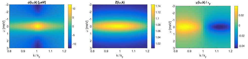
In Fig. 11 we plot the solutions of Eqs. 5 of the main text restricted to a smaller region near with larger , and with the same parameters except for . This solution represents a typical solution for the experimental parameters, and thus represents the self energy for the case of the most dilute superconductor reported in Ref. Lin et al. (2013).
The weak coupling behavior of motivates us to seek a simpler description of the self-energy which is restricted to the Fermi surface. This is obtained by integrating the dispersion in the denominator and the Coulomb interaction analytically over in the region , where is the cutoff (we use in our calculations, however the results are not very sensitive with respect to the cutoff). We also note that as the coupling is reduced the dispersion renormalization becomes smaller and smaller compared to , and therefore we neglect it.
The resulting isotropic Eliashberg equations are given by
| (22) | |||
where and the functions
and
diverge logarithmically at small frequency like and , and go to zero like at large . Here . The logarithmic divergence is the main difference compared to standard Eliashberg theory and is a result of the un-screened Coulomb interactions.
V Calculation of the transition temperature
At the solutions of Eq.(22) go to zero and decouple and therefore, if we are interested only in the transition temperature we can linearize Eq. (22)
| (23) |
where . can be found by seeking when the largest eigenvalue of becomes unitary. The main advantage of this method is that it involves linear manipulations instead of seeking a solution to the non-linear equation. As a result it is much more stable to large values of .
In Fig. 1 in the main text we plot calculated for two different set of parameters. The blue curves corresponds to , , and and the cyan ones to , , and . We also plot the resulting frequency , the Fermi energy and the frequency of the transverse mode in Fig. 1.b and Fig. 1.c of the main text.
VI The transition temperature in two-dimensions
In this section we discuss superconductivity in two-dimensional electronic gases based on SrTiO3 (for example, the LaAlO3/SrTiO3, Nb -doped SrTiO3 and gated SrTiO3).
VI.1 Paring interaction
As in 3d, we assume a single resonance model for the dielectric constant
| (24) |
However, in this case we will assume that the soft mode has completely stiffened and is given by [cite Reinle-schmitt], such that .
The 2D polarization bubble of a single band with mass has the form
| (25) |
where and and . The RPA interaction is then given by
| (26) |
where . The plasma frequency is now strongly -dependant and is given by
| (27) |
Just as in the case of three-dimensions, in the limit we can separate the interaction into two resonances
| (28) |
| (29) |
| (30) |
and .
We may consider two distinct limits. In the limit we can simply substitute instead of . On the other hand if than the -dependant plasma frequency crosses through the optical phonon mode as is integrated from to roughly , and therefore goes to zero. For the typical Fermi energies in the STO-based 2d gases the latter case holds. As a result the coupling will suppress the contribution from the lower the mode for .
On the other hand the plasma oscillations appear only in the limit or . Comparing these restrictions we find that if than goes to zero much before becomes larger than . We therefore argue that the interaction can be approximated by the plasmon pole approximation
| (31) |
VI.2 Linearized Eliashberg equations
Just as in 3d we linearize the Eliashberg equations
| (32) |
where
and
where we have restricted the integration close to the Fermi momentum (assuming that the coupling is weak we take ) and we taken into account the finite value of the interaction at as in Fig. 2. Note that here the average over the angle of is performed numerically because both and are funcitons of .
As before we have the eigenvalue problem
| (33) |
where the matrix is given by
| (34) |
where the Matsubara frequencies and are spaced by and run up to some cutoff. is obtained when has an eigenvalue of unity. In fact, corresponds to the temperature where the largest eigenvalue of becomes unity.
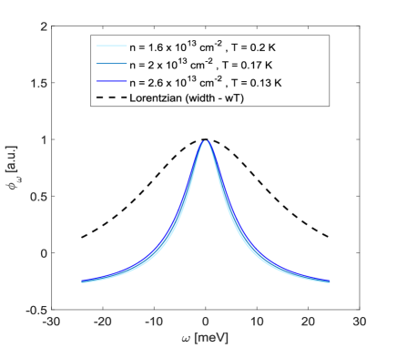
The resulting for , and various ’s is plotted in Fig. 3. In Fig. 13 we also plot the eigenvector at with and for three different densities corresponding to Fermi energies of . The dashed line is a Lorentzian shape with width for comparison. As can be seen, the width of the , which mimics the width of the retarded interaction is approximately . Therefore it is significantly smaller than (and also ). This justifies the use of a small at the typical range of densities where superconductivity is observed. Indeed we expect the width of the interaction in frequency space to be significantly smaller than because most of the weight in the angular integral comes from small where . We also note that the shape is not exactly a Lorentzian (namely, it has long tails).
VII Analytic continuation of the self-energy
In this section we elaborate on the controlled Padé approximation Beach et al. (2000) used to analytically continue the self-energy in the Green’s function (Eq. 6 in the main text) to the real axis. From Eq. 22 we obtain the functions and in a finite number of fermionic Matsubara frequencies lying in the region . There is no unique analytic continuation of a finite set of points to the entire upper half plane. The Padé form
| (35) |
where
and
is often used because it posses all the analytic properties of a response function in the upper half plane. This statement is actually true under the condition that is real and positive. Therefore, Ref. Beach et al. (2000) has proposed to use the imaginary part of as a control parameter to quantify the quality of the analytic continuation. Following Ref. Beach et al. (2000), we analytically continue from Matsubara points which, i.e. (note that need not be the full number of Matsubara frequencies for which and is known). The coefficients of these polynomials are obtained by solving a linear set of equations
for the set of Matsubara points . The imaginary part of is monitored and found to be smaller than numerical precision in all calculations.
VIII the tunneling density of states in a dilute superconductor
Given the analytic continuation of the of the self-energy Eq. 35 we can now calculate the single-particle density of states from the imaginary part of the electron’s Green’s function Schrieffer et al. (1963)
| (36) |
In the case of a shallow band () this gives
| (37) |
where is the density of states at the Fermi level, , and we have neglected the momentum dependence of the gap and the density of states coming from the smaller Fermi pockets.